Human Choice Prediction in Non-Cooperative Games: Simulation-based Off-Policy Evaluation

Abstract

Persuasion games have been fundamental in economics and AI research, and have significant practical applications. Recent works in this area have started to incorporate natural language, moving beyond the traditional stylized message setting. However, previous research has focused on on-policy prediction, where the train and test data have the same distribution, which is not representative of real-life scenarios. In this paper, we tackle the challenging problem of off-policy evaluation (OPE) in language-based persuasion games. To address the inherent difficulty of human data collection in this setup, we propose a novel approach which combines real and simulated human-bot interaction data. Our simulated data is created by an exogenous model assuming decision makers (DMs) start with a mixture of random and decision-theoretic based behaviors and improve over time. We present a deep learning training algorithm that effectively integrates real interaction and simulated data, substantially improving over models that train only with interaction data. Our results demonstrate the potential of real interaction and simulation mixtures as a cost-effective and scalable solution for OPE in language-based persuasion games.

1 Introduction

Context: Human Choice Prediction in Non-Cooperative Games

Much research in artificial intelligence (AI) and particularly in reinforcement learning (RL) has long focused on designing agents that can play games [19]. However, most games studied in this context are zero-sum and are typically modeled as a utility maximization problem [22]. This is in contrast to economic games, which are generally non-zero-sum. For instance, a commerce website that recommends a hotel to a customer is concerned with the customer’s choice of hotel, whereas the customer is interested in the quality of the recommended hotel. Although the incentives of the two parties are distinct, they are not opposite, and hence such games cannot be solved through maximization. In fact, there is no optimal player in such problems [13]. While communication among agents in economic games is typically through formal signals [2, 16], we direct our attention to natural language communication, which is natural in persuasion games.

[1] introduced a novel adaptation of the aforementioned setup to natural language messaging, where they designed a multi-stage persuasion game involving an expert (travel agent) and a decision-maker (DM, customer). In each interaction, the expert is presented with a hotel and its scored textual reviews and must choose a single review to reveal to the DM, with the aim of convincing her to choose the hotel. The DM can either accept or reject the hotel, and her payoff is determined stochastically based on the review score distribution, available only to the expert. After observing their payoffs, both players proceed to the next, similar step of the game, which differs from the previous steps only in the hotel presented to the expert. While [1] focused primarily on predicting the DM’s actions, [20] adapted this framework and designed an artificial expert (AE) to perform the expert’s roles in a manner that attempts to maximize the number of accepted hotels by the DM. Their AE has incorporated the Monte Carlo Tree Search (MCTS) algorithm [10], utilizing deep learning models that take advantage of behavioral and linguistic features to anticipate the decision maker’s subsequent action, along with the anticipated future reward of the expert based on the game’s status and a potential review.

While the above is promising, in an economic context predicting behavior is not an optimization problem. Indeed, this is inherent in the fact we refer to general non-cooperative games rather than to zero-sum games. Therefore, the best we can hope for is to try and predict how a human DM would behave when interacting with an unseen expert (bot). We hence introduce the study of off-policy evaluation (OPE) for experts when interacting with human DMs in a non-cooperative game.

Our games will be like the persuasion games above, which are fundamental to economic theory ([16], following [2]), a variant of which also discussed in machine learning applications like segmentation [11] and exploration-exploitation [3]. The current study extends the work of [1] to the problem of OPE, i.e., relaxing the assumption that human DMs face the same experts at both train and test times. By using OPE, a strategy profile to be tested consists of an untried bot expert matched with an unseen DM, and our aim is to predict the DM’s decisions. Notice that our approach provides a solution to outcome prediction in non-cooperative games: we try to predict behavior of strategies which were not played yet, based on past behaviors.

What: OPE

Given data on a 2-player non-cooperative game played by human-bot pairs, we aim at predicting (other) human behavior when playing with (other) bots. As the interaction is through a multi-stage action-feedback setting, this problem can be viewed as an OPE challenge in an offline RL context. However, as we study a non-cooperative, non-zero-sum game, our aim is not to optimize behavior (through, e.g., regret minimization) but to accurately predict human choices.

Our work contributes to OPE methods in the offline RL literature [24, 6, 12, 18, 29]. While formalisms take different forms, in all such settings we have a dataset of traces/trajectories of agent-environment interactions (potentially derived by the use of various policies in an MDP setting), and the aim is to evaluate a previously unobserved (or find optimal) policy for the agent in that environment. In our setting, we have traces of previous interactions between experts (i.e., policies, bots) and DMs in a non-cooperative game. More specifically, we have a dataset consisting of a sequence of $n$ pairs $(e_{i},d_{i}),1\leq i\leq n$ of expert policy $e_{i}$ and trajectory observed when playing $e_{i}$ with a DM $d_{i}$, in a given non-cooperative game. Our aim is to predict the play of a (previously unseen) DM $\bar{d}$ facing an (untried) expert $\bar{e}$ in that non-cooperative game. In service of OPE in this setting, we will introduce a simulation-based approach that aims to enhance the robustness of our decision prediction model.

How: Mixing Interaction Data with DM Simulation

How do we go for this high-bar challenge? In this paper, we introduce a novel use of mixing interaction data, as in offline RL, with simulations of bot-DM interactions. Rather than appealing only to typical psychological-theoretic models (like prospect theory [15]) of DMs in our simulations, we incorporate an exogenous DM model, which is based on the assumption that DMs start from some behavior, which may combine random behavior and some decision-theoretic based behavior, and become better players over time. The improvement-over-time principle is independent of any specific bot or game, and hence it allows us to generate valuable data from interactions between simulated DMs and a large variety of bots. Training a human decision prediction model from a mixture of simulated and human-bot interactions hence results in a more robust model, that is not fitted to the idiosyncrasies of the bots in the human-bot interaction training set. Such robust models are more suitable to make predictions for new bots and human DMs.

Simulation ideas have been flowering in the field of RL, with several successful applications. Notably, the self-play algorithm proposed by Tesauro [23] has emerged as a particularly powerful idea in this context. Simulation has also played a key role in RL for robotics [5, 25], and has gained traction in the training of autonomous cars [28]. One challenge of simulation-based learning is the potential mismatch between the simulation and the real world, which can lead to poor performance when the model is deployed in the target environment. As noted above, we overcome this challenge by basing our simulation on a DM model whose core idea, that the DM learns to make the right decisions over time, is independent of any specific bot or game.

Our work contributes a novel use of integrating interaction-data with simulation-data. Doing this we step in the footpath of several works in diverse domains (e.g. natural language processing [7], autonomous cars [8, 28], and astro-particle physics [21]). As noted above, our novelty is in exploiting an exogenous model of decision-maker learning dynamics in an economic context, as captured by language-based non-cooperative games.

In order to empirically explore our game, we implemented a mobile application that allowed us to collect data at scale (Section 3). Particularly, our dataset consists of 85,858 decisions from 244 DMs who played against 12 different automatic expert bots (each DM played against 6 bots). We consider this dataset as a contribution to the research community and will make it public, hoping that it will promote the research in our area.

The findings from our study indicate that incorporating simulated and real-world data of bot-DM interactions leads to superior performance compared to solely relying on real-world (or simulation) data. Specifically, our results show an improvement of more than 5% in prediction of challenging examples when using simulation during model training, compared to using only interaction data.

2 Problem Definition

While the space of non-cooperative games is very large, our emphasis here is on language-based games, in which textual messages replace the stylized messages discussed in economic theory. On the other hand, as we wish to consider fundamental economic language-based games and to follow the very recent literature [1], we focus on what is taken as the central sender-receiver setting: persuasion games. Indeed, we aim to focus as much as possible on the same game structure as studied in that recent literature.

Language-Based Persuasion Game

Based on [1], we consider a problem involving a multi-stage game between two parties: the sender (referred to as expert) and the receiver (referred to as decision-maker or DM). The game consists of R rounds. In each round, the expert, which plays the role of a travel agent, attempts to promote a randomly selected hotel. The expert is presented with SR scored reviews that were written and scored by real users of Booking.com. The expert is then asked to send the DM one of the reviews to persuade her to select the hotel. An example review is presented in the supp. material. A hotel is considered "good" if $\hat{s}=\frac{1}{SR}\sum\limits_{i=1}^{SR}s_{i}\geq TH$ (i.e. its average review score, $\hat{s}$, is not less than a predefined threshold, $TH$) and "bad" otherwise, where $s_{i}$ is the hotel’s $i^{\prime}th$ score.

In the experimental study (see next section), following [1], we take R=10 and SR=7. We chose TH=8.0 because, according to Booking.com, a hotel rated 8.0 or higher is considered a "good hotel". The definition of what constitutes a good hotel is available to the expert but not to the DM.

While the expert observes both the verbal and the numerical part of the reviews and therefore knows whether the hotel is good or not, the DM observes only the verbal part of the review sent to her. The DM’s task is to decide whether to accept the expert’s offer and go to the hotel or decline it and stay at home, based only on the review provided by the expert. The DM’s payoff at each round depends on the quality of the hotel, with a positive payoff received when a good hotel is selected or when a bad hotel is not selected, and a negative payoff incurred otherwise. At the end of each round, both players are notified of the DM’s decision and his individual payoff.

Strategy Space

To crystallize the input structure and the bots to be experimented with and tested during OPE, we determine the Strategy Space. This space encompasses all simple, deterministic decision-tree-based strategies that can be constructed using a pre-defined set of binary split conditions and a pre-defined set of actions. These conditions and actions are based on the respective reviewers’ numerical scores assigned to the hotels, and the game’s history, as detailed in Table 1. Employing decision trees of depth up to 2 (to keep the strategies simple to understand for a human player), we obtained a total of 1179 distinct strategies. Six of these strategies were selected for group $E_{\mathcal{A}}$, and six others for group $E_{\mathcal{B}}$. The strategies that were selected are (a) diverse from one another; and (b) reflect the preference of the bot that the DM would select as many hotels as possible. One example of such a strategy is presented in Figure 1. A full list of the strategies in $E_{\mathcal{A}}$ and $E_{\mathcal{B}}$ is in the supp. material, alongside a justification as to why they respect the above criteria.

Our challenge: Given a dataset comprising of interactions between human decision-makers and an ordered set of rule-based experts $E_{\mathcal{A}}$, our objective is to predict the behavior of other human decision-makers when they engage in game-play with another ordered set of rule-based experts $E_{\mathcal{B}}$.

Table 1: The conditions and actions employed by the rule-based experts in round $t$. The hotel score in the $i$-th round is denoted with $\hat{s}_{i}$, while the binary decision made by the decision maker in the $i$-th round is denoted with $d_{i}$ (with $d_{i}=1$ for hotel selection).

Split Condition Description	Condition formulation
Is the current hotel good?	$\hat{s}_{t}\geq 8$
Did the DM choose to go to the hotel in the
previous round?	$d_{t-1}=1$
Was the hotel in the previous round good?	$\hat{s}_{t-1}\geq 8$
Has the decision maker earned more points than the
number of times he chose to go to the hotels?	$\sum_{i=1}^{t-1}(I_{\hat{s}_{i}\geq 8}=d_{i})>\sum_{i=1}^{t-1}d_{i}$
Action Description
Send the $r$ review	$r\in$ {best, mean, worst}

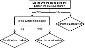
Figure 1: An example of a strategy from the $E_{\mathcal{B}}$ set.

3 Human-Bot Interaction Data Collection

In order to collect data, we developed a mobile phone game that follows the above multi-stage language-based persuasion game setting. In our game, a human DM plays with a series of 6 rule-based experts (bots), each game consisting of 10 rounds. The DM gets 1 point if she makes a good decision (selecting a good hotel or avoiding a bad one), and 0 points otherwise, and hence the maximal payoff is 10. To advance to the next level (play with the next bot), the DM must achieve a pre-defined target payoff. The target payoffs are in the 8-10 range, and are defined according to how challenging the bot is. The goal of the human player is to get the target payoff of all six experts. We refer to reaching the target payoff as "defeating" the expert, although this is not a zero-sum game with adversarial experts.

The hotels

Utilizing hotel reviews sourced from Booking.com, we compiled a dataset comprising 1,068 hotels, each with $SR=7$ scored reviews. We chose the hotels so that only about half of them are defined as good (i.e., $\hat{s}\geq TH=8$). The median score of the hotels was also set to 8.01.

Interaction Data

We ran our game in Apple’s App Store and Google Play for a few months (May 2022 - January 2023). The players who downloaded the app until November 2022 played with group $E_{\mathcal{A}}$ experts, while the players who played from December 2022 played with group $E_{\mathcal{B}}$ experts. We collected 85,858 decisions taken by 244 players who finished the game, i.e., defeated all six experts. Statistical details of the data are given in Table 2. We used reward schemes, including lottery participation and course credit, to incentivize players to beat all six experts in the game. More details about our app and the data collection process are in the supp. material.

Table 2: Dataset Statistics

Group	Experts	#DMs	#decisions	median #decisions/DM	median #games/DM
A	$E_{\mathcal{A}}$	210	71579	273	33.5
B	$E_{\mathcal{B}}$	34	14279	337.5	51.5

4 Simulation-Based OPE in Language-Based Persuasion Games

The basic algorithmic idea we introduce is a simulation of the overall space of joint strategies, i.e., (bot, agent) pairs behavior. We mix this simulation data with human-bot interaction data in service of bridging to previously unseen situations (i.e. performing OPE with unseen bots and DMs). Our simulation of the DM introduces an additional ingredient - incorporating an exogenous model of learning behavior by the DM - namely capturing the axiom that a learning agent gradually learns to behave "right" (rather than say how exactly it learns; this component of the DM model is independent of any specific bot or game).

Particularly, to improve prediction accuracy in the OPE task, we generated a simulation dataset consisting of games played between simulated DMs and experts, so that the participating experts span the entire Strategy Space. This section describes the process we use to generate the simulation data and the way we integrate the interaction and the simulated data in the training process of a DM behavior prediction model.

The Simulation

In each instance of the bot-DM interaction simulation, we randomly select six expert strategies from the strategy space. For each simulated DM-bot interaction, we randomly sample 10 hotels, one for each of the $R=10$ rounds. In each of the rounds, the expert uses its strategy to select a review from the review set of the hotel associated with that round. The simulated DM uses the textual content of the review and its estimated numerical score to make her decision. Notice that as opposed to the real human-bot interactions, in the simulation the DM model does use the numerical score of the review. However, in order to emulate the reality where it is hard for humans to accurately estimate the review score from its text, the estimated numerical score is defined as $\hat{s}+x$, where $\hat{s}$ is the actual score of the review and $x~{}\sim Normal(0,\epsilon)$ is a noise variable. The simulation involves the DM playing the 10 rounds game against the same expert until achieving a payoff of $SIM\_PAY\_TH=9$ points, before moving on to play against the next expert.

Our simulation is based on two basic probability vectors: (a) The nature vector, a hyper-parameter vector denoted with $(p_{1},p_{2},p_{3})$; This vector provides the initial probabilities that the DM will select one of three basic strategies (see below); and (b) The temperament vector, comprised of four values $(p_{0}^{t},p_{1}^{t},p_{2}^{t},p_{3}^{t})$ and updated in each round $t$. While $p_{1}^{t},p_{2}^{t},p_{3}^{t}$ correspond to the three values in the nature vector, $p_{0}^{t}$ is the probability that the DM will take the right decision just because it has learned how to play the game from the multi-stage interaction with the bot.

The nature vector is based on three strategies: Trustful, Text-based, and Random. These strategies reflect the two basic components we attribute to a DM: considering past behavior and its outcome (Trustful) and learning from the information in the current hotel’s review (Text-based), alongside the inherent randomness in human behavior (Random). Under the Trustful strategy, the DM chooses to go to the hotel if and only if in the last $K$ rounds the DM’s estimated review score matched the feedback about the hotel quality, where $K$ is a stochastic parameter sampled for each DM individually. According to the Text-based strategy, the DM modifies its estimated numerical hotel score (see above) by adding or subtracting points based on certain textual features of the review. In order to create diverse DMs, these features are randomly selected for each DM from the set of textual features defined by [1] for their human decision prediction model. Finally, under the Random strategy, the DM would make a random decision.

The temperament vector is initialized at the onset of each 10-round DM-bot interaction to be:

$$temperament\_vector(t=0)=(p_{0}^{0}=0,p_{1}^{0}=p_{1},p_{2}^{0}=p_{2},p_{3}^{0}=p_{3})$$ (1)

where $p_{0}^{t}$ represents the probability of making the right decision. At each round $t$, the temperament vector is updated by multiplying $p_{1\leq i\leq 3}^{t}$ by a factor of $1-\gamma_{i}^{t}$ (the DM’s learning rate), where:

$$\gamma_{i}^{t}\sim Uni(-\frac{\eta}{10},\frac{9\eta}{10})$$ (2)

and $\eta\in(0,10/9]$ is a hyper-parameter representing the DM’s improvement. Accordingly, $p_{0}^{t}$ is updated to be:

$$p_{0}^{t}=1-\sum_{1\leq i\leq 3}p_{i}^{t}$$ (3)

to ensure that the temperament vector is a probability vector. In this way, the temperament vector after $T>0$ rounds is defined by:

$$p_{1\leq i\leq 3}^{T}=p_{i}\prod_{t=1}^{T}(1-\gamma_{i}^{t})\quad\mathrm{and}\quad p_{0}^{T}=1-\sum_{1\leq i\leq 3}p_{i}^{T}$$ (4)

Since $0<E[1-\gamma_{i}^{t}]<1$, it holds that the probability making the right decision ($p_{0}^{T}$), irrespective of the nature vector, tends towards 1 as the number of rounds approaches infinity. Hence, the DM will inevitably defeat any expert after a sufficient number of rounds.

Gradient-based Training

We leverage both simulation data and real human-bot interactions to train the decision prediction model. The simulation data serves two distinct purposes during the training process. First, it is used in order to initialize the model as a pre-training step. This involves training the model with $S_{pt}$ simulated DMs at the outset of the training process. Second, at the beginning of each training epoch, we further train the model using $S_{e}$ simulated DMs, and subsequently train the model using the human-bot interaction data ($S_{pt}$ and $S_{e}$ are hyper-parameters).

The pseudo-code of the simulation and the training algorithm is in the supplementary material.

5 Experiments

5.1 Feature Representation

We represent each DM-bot interaction round with features related to (1) the hotel review sent by the expert to the DM; and (2) the strategic situation in which the decision was made. To represent a review, we utilize a set of binary Hand Crafted Features (HCFs) originally proposed by [1]. These features describe the topics that the positive and negative parts of the review discuss (for example: Are the hotel facilities mentioned in the positive part of the review?) as well as structural and stylistic properties of the review (for example: Is the positive part shorter than the negative part?). To label the topics the review discusses, we use OpenAI’s Davinci model. The model receives as a prompt the review and the feature definition as in [1], and is asked to indicate whether or not the feature appears in the review. As in [1], the use of HCFs yielded better results compared to deep learning based text embedding techniques such as BERT [17]. To represent the strategic situation, we introduce additional binary features that capture the DM’s previous decision and outcome, current payoff, and frequency of choosing to go to the hotel in past rounds of the same interaction. A full list of the features is in the supplementary material.

5.2 Models and baselines

This subsection provides a description of the models that we train for our study. For each model, except for the Majority Vote model, we train two versions: one using only interaction data and the other with both interaction and simulation data. This allows us to evaluate the impact of simulated data on the model’s predictive performance. All the models are designed to predict the DM’s decision in a specific round, given the previous rounds played in the same bot-DM interaction.

Majority Vote

The Majority Vote baseline predicts the DM’s decision based on the percentage of DMs who decided to go to the hotel in the interaction training set. Notably, this baseline method solely relies on the review and disregards the repeated nature of the game. Additionally, it is unsuitable for predicting the decisions of players who are the first to encounter a new review. In order to make sure that we consider only cases where DMs indeed read the review, we consider only cases where DMs spent at least 3 seconds before making their decision. .

Machine Learning Models

we employ three machine learning models to predict the DM’s decisions. First, we utilize a Long Short-Term Memory (LSTM) model [14], wherein the cell state is initialized before the DM’s first game (10-round interaction with a bot) to a vector estimated during training, while the hidden state is propagated from game to game. By managing the cell state in this manner, we model the relationship between successive games of the DM against the same expert. Second, we train a Transformer model [26] that takes as input the representation of all rounds up to round $t$. Lastly, we implement the XGBoost Classifier [9], a strong non-neural, non-sequential model. The hyperparameter tuning procedures and technical information of the training process are provided in the supplementary material.

Ablation Baselines

Experiments with these baselines aim to shed light on the factors that contribute to the positive impact of the simulation. To this end, we consider three variants of the simulation process of Section 4. First, we examine the effect of modeling the DM’s behavior on learning by initializing it as a random DM, i.e., setting the nature vector to be $(p_{1}=0,p_{2}=0,p_{3}=1)$. Then, we test the impact of the DM’s learning over time on model performance by setting the DM improvement parameter ($\eta$) to zero. Last, we explore the combination of both changes.

5.3 Research Questions

We consider the following research questions: Q1: Does incorporating simulation data during model training improve the accuracy of decision prediction in OPE scenarios? Q2: Does simulation improve different types of learning models? Q3: What are the components of the simulation that lead to the improved results? Q4: Is the effect of simulation inherently connected to the OPE setup? Can it also help when the OPE challenge is relaxed (e.g. when only the test-time DMs are new while test-time bots are the same as those of the training)? We next present our answers to these questions.

6 Results

In this section we report the results of each model as the mean of the average accuracy per player (DM). We average over DMs rather than over decisions so that human DMs that played more games than others are not over-represented in the results.

The impact of the simulation (Q1 and Q2)

Table 3 (top) presents the performance of all models, with and without simulation data. Notably, LSTM performs best, serving as the optimal model for the prediction task. This finding is in line with [1], which demonstrated that LSTM is the most suitable model for predicting decisions in language-based persuasion games in the on-policy setup.

Table 3: Top: Average accuracy of each model by expert strategy (Q1 and Q2), with "+S" indicating models trained using both simulation and interaction data. TF = Transformer. Maj = Majority. LSTM OS = LSTM trained with simulation data only. The best-performing model is highlighted in bold. Expert strategies are listed in the order of their appearance during the game. Bottom: Performance of the various models when predicting decisions where the confidence level of the column model is at least 20% for both classes. The results demonstrate that incorporating simulated interactions in the training process improves the accuracy of the models for each subset of challenging decisions, as compared to model variants that are trained with human-bot interactions only.

Model \ Expert	#1	#2	#3	#4	#5	#6	Average
LSTM+S	85.47%	80.93%	90.27%	82.51%	79.66%	86.71%	84.26%
LSTM	84.59%	80.12%	88.88%	82.12%	78.59%	85.17%	83.24%
LSTM OS	84.85%	71.63%	87.22%	76.38%	71.15%	81.38%	78.77%
XGBoost+S	86.13%	78.82%	88.68%	82.3%	77.92%	86.46%	83.38%
XGBoost	85.43%	78.72%	87.82%	82.32%	76.23%	86.1%	82.77%
TF+S	84.38%	78.3%	88.57%	81.71%	77.07%	84.54%	82.43%
TF	84.26%	78.83%	87.67%	81.35%	76.61%	84.88%	82.27%
Majority	85.13%	72.2%	85.89%	79.06%	70.72%	80.46%	78.91%

\ Hard to	Maj.	XGBoost	LSTM+S	LSTM	TF	All	One
Accuracy of \						Baselines	Baseline
LSTM+S	70.55%	72.15%	61.68%	64.56%	66.45%	59.68%	72.74%
LSTM	67.76%	67.44%	57.16%	58.69%	62.01%	56.17%	70.11%
XGBoost+S	68.66%	68.26%	60.72%	62.9%	62.56%	57.64%	71.09%
XGBoost	66.82%	65.6%	60.22%	62.26%	62.53%	54.43%	69.9%
TF+S	66.45%	66.18%	57.4%	59.11%	59.87%	56.77%	68.97%
TF	66.1%	66.3%	55.86%	58.4%	59.39%	56.86%	68.44%
Majority	62.43%	63.37%	58.08%	59.67%	58.57%	55.17%	64.67%
# Decisions	3568	4490	3898	4085	4502	957	7694
% tot. Dec.	24.99%	31.44%	27.3%	28.61%	31.53%	6.7%	53.88%

Models trained on a mixture of interaction and simulation data were exposed to strategic situations between DMs and experts that were not observed in the interaction data. Despite the synthetic nature of the simulation data, it enhanced the learning of the model, and yielded improved predictions of previously unseen DMs’ behavior when playing against experts from $E_{\mathcal{B}}$. The simulation was particularly effective for the LSTM model, with an average performance gain of 1.02% compared to training with interaction data only. Other models, such as XGBoost and Transformer, lagged behind, with a less pronounced but still positive effect of the simulation.

Enhancing Prediction Accuracy with Simulation Data in Challenging Cases (Q1 and Q2)

We analyze the performance of our models in predicting actions under varying levels of difficulty. Our main focus is on scenarios that are challenging to each of the various models we consider. For Table 3 (bottom), we define a decision as challenging for a given model if the probability the model assigns to the two possible actions is at least 0.2. It shows that the LSTM+S model surpasses each of the models trained solely on interaction data by a margin of at least 5% on their hard-to-predict examples. Moreover, it is noteworthy that the LSTM+S model outperforms all interaction-data-only models by at least 1.45%, even on examples that it finds challenging. Furthermore, we observe that incorporating simulation data into XGBoost improved its predictions on its own challenging examples by 2.76% (XGBoost+S compared to XGBoost, in the XGBoost column). These results suggest our simulation is advantageous in enhancing prediction accuracy across models, particularly in the challenging cases. Figure 2 provides results for additional minimal per-class confidence levels.

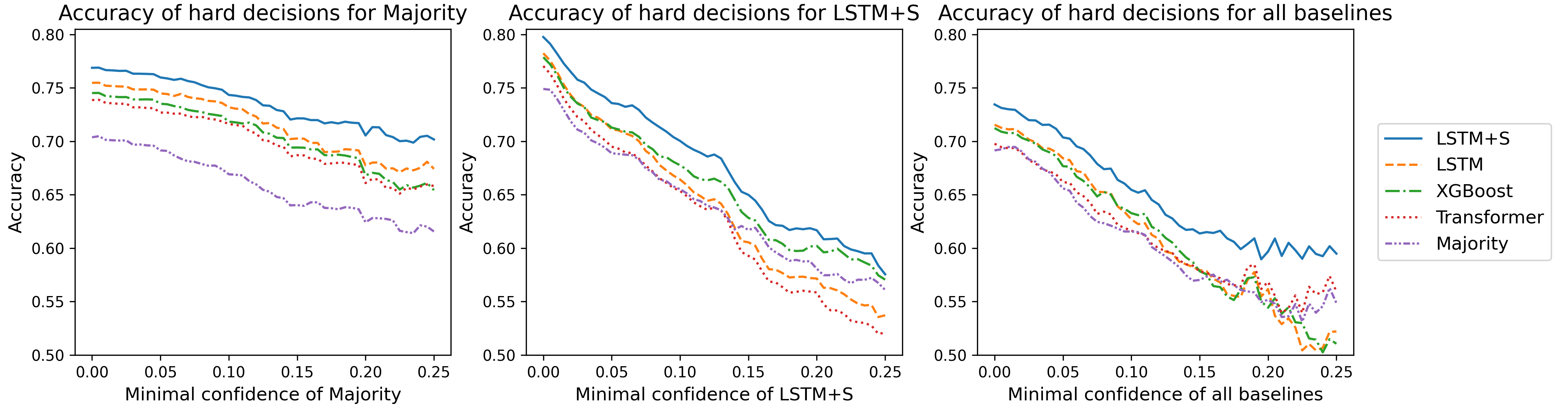
Figure 2: Model performance as a function of the confidence level of various models.

Ablation Analysis (Q3)

We start by asking whether our models can be effectively trained with simulation data only, without access to human-bot interaction data. AS demonstrated by the reduced performance of the LSTM OS model (Table 3 (top)), the answer to this question is negative. We conclude that the impact of simulation is in its combination with the human-bot interaction data (we observe similar patterns for the other models).

We next explore which component of the simulation is most important for improved behavior prediction (Figure 3). We observe that the improvement of DM over time ($p_{0}^{t}$) has a greater impact on prediction accuracy than the behavioral ($p_{1}^{t}$) and textual ($p_{2}^{t}$) aspects of the simulation. Yet, these aspects of the simulation have a complementary effect, as the simulation achieves its best impact when all components are integrated. Moreover, simulation that covers the entire strategy space facilitates learning better than when considering the $E_{\mathcal{B}}$ (i.e. test-time) strategies only. We see the latter observation as an indication of the regularization effect of the simulation.

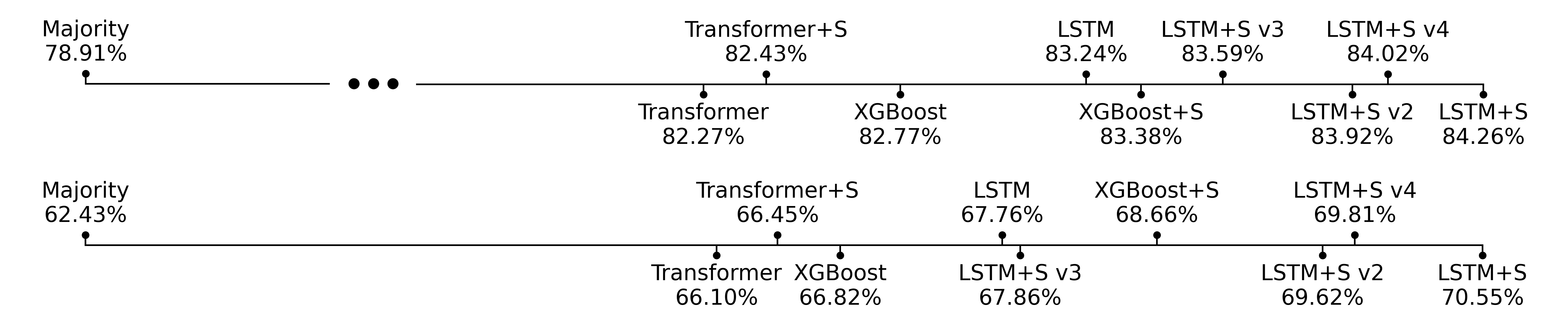
Figure 3: Ablation analysis of the impact of the different components of the simulation. We consider the simulation without the behavioral and textual components ($p_{1}=p_{2}=0$, V2), or when the simulated DM does not improve over time ($\eta=0$, V3), or when the experts in the simulation are the $E_{\mathcal{B}}$ strategies (V4). Top: All examples. Bottom: challenging examples for Majority.

Relaxed OPE performance (Q4)

We hypothesized that the simulation improves decision predictions for unseen DMs and bots because it keeps the model from overfitting to the $E_{\mathcal{A}}$ strategies and the training-time DMs. But what happens when only the DMs change at test-time, and the bots are kept unchanged (i.e. when evaluating different DMs on the $E_{\mathcal{A}}$ strategies)? To answer this question we trained the LSTM model with data from 80% of the human DMs who played against $E_{\mathcal{A}}$ bots and tested that model against the other 20% of the human DMs, and observed that the simulation improved the performance by 1.05% (from 81.38% to 82.43%). This result is in line with previous ML work (e.g. [4, 27]) which demonstrated that algorithms designed with out-of-distribution improvement in mind also improve performance when the train and test distributions are more similar to each other.

7 Discussion and Limitations

We introduced the challenge of OPE in non-cooperative, language-based persuasion games. We propose a simulation in which DMs make the correct decision with a progressively increasing probability. Training DM decision prediction models with a mixture of simulation data and human-bot interactions yields substantial gains.

In service of addressing the challenge of OPE in language-based persuasion games, we made several restricting assumptions. While our strategy space is rigorously defined and allows us to crystallize the approach, considering more involved strategies (bots) is a natural extension in bridging this topic into practice. In addition, while we believe introducing our challenge and solution in the framework of language-based persuasion games, as discussed in recent literature, is a natural starting point, extending the study to other language-based games may be a tempting future challenge.

Finally, we would ideally aim to demonstrate results for a wide range of strategy sets that would serve as $E_{\mathcal{A}}$ and $E_{\mathcal{B}}$, and with a larger variety of parameters (e.g., for games with a larger number of rounds). However, since data collection from humans is costly and laborious, we restrict our experiments to a specific choice of $E_{\mathcal{A}}$ and $E_{\mathcal{B}}$, potentially affecting the generality of our findings.

Predicting human behavior is a classical case of technology that can be abused for a range of malicious goals. This research can hence be used with caution, and we hope that the benefits will outweigh the potential harm.

Appendix A Game Strategies

In this appendix, we present the expert strategies of groups $E_{\mathcal{A}}$ and $E_{\mathcal{B}}$ of our game. The formal mathematical notations of the tree node conditions are provided in Table 1 of page 4 in the main paper.

Figure 4: The strategies of the $E_{\mathcal{A}}$ experts.

(a) 1st expert’s strategy

(b) 2nd expert’s strategy

(c) 3rd expert’s strategy

(d) 4th expert’s strategy

(e) 5th expert’s strategy

(f) 6th expert’s strategy

Figure 5: The strategies of the $E_{\mathcal{B}}$ experts.

(a) 1st expert’s strategy

(b) 2nd expert’s strategy

(c) 3rd expert’s strategy

(d) 4th expert’s strategy

(e) 5th expert’s strategy

(f) 6th expert’s strategy

Appendix B Data Collection

B.1 Hotels Dataset

As described in Section 2 of the main paper, our dataset encompassed seven reviews for each of a total of 1068 hotels. The complete dataset can be found in the ’data/game_reviews’ directory of the code folder attached to our supplementary material. Figure 6 provides a representative review example.

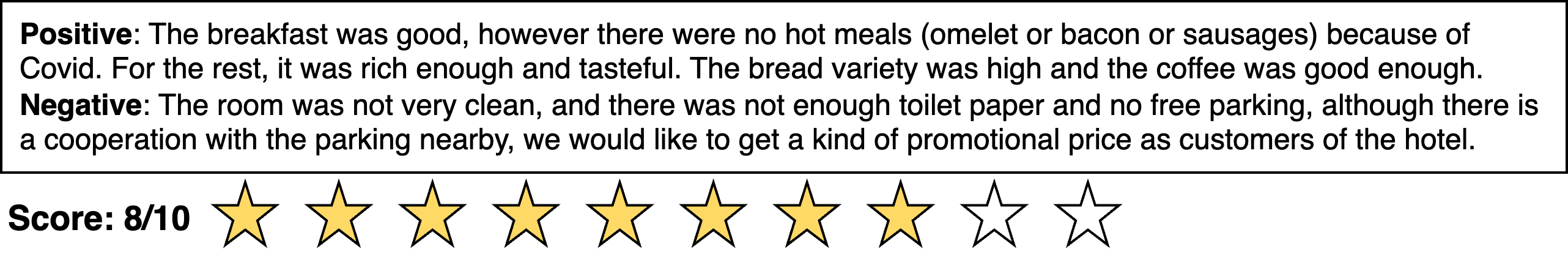
Figure 6: A sample review from our hotel review dataset.

B.2 Instructions

The following quote contains the instructions given to players in the app stores.

Are you the vacation planner at your house? Think you always know how to choose the best hotel? Start to plan your 10-days trip with our travel agents. Just remember - they don’t always want the best for you, and might have their own strategy to make you book the hotel they try to promote!

Travel or Trouble is a strategy game in which you will try to outsmart our traveling agents and plan the perfect vacation for you.

Each game consists of 10 rounds, in each round, one of our traveling agents will introduce you with a review for a new hotel they think might suit you, and you will have to choose: either book the hotel or stay home.

Only true vacation masters can identify a good hotel based upon one review… are you up to the challenge???

As in life, each vacation can turn out to be a great success or a huge disappointment.

Once you made your choice, you will see the results for the vacation in question: was it good or bad?

Based upon the hotel’s average rating (to which only the expert is exposed, and is based on multiple reviews for each hotel), a lottery will determine the outcome of the vacation.

Collect points either by choosing a hotel that turned good or by avoiding bad ones.

Remember - the travel agent is rewarded each time you choose a hotel, regardless of the outcome!

At each game, you will meet a different agent, with a different skill of persuasion.

Try to discover each of our agents’ strategies to persuade you, and take the right decision every round.

Advance through the world of traveling by earning achievements on your way to becoming the true vacation master.

B.3 App Screenshots

In this appendix, we provide several screenshots from our data collection application.

(a) Home Screen	(b) Instructions	(c) An Agent introduces
		himself

(d) Positive feedback after	(e) Negative feedback after	(f) Positive feedback after
going to a good hotel	not going to a good hotel	not going to a bad hotel

(g) Negative feedback after	(h) A signal sent by the agent	(i) Agent selection screen
going to a bad hotel

B.4 Information about the human players

As section 3 of the article describes, the app has been available on Google Play and Apple App Store for several months. To attract participants, we also published the app on social media. To increase participation and game completing (playing until defeating all six experts), in some publications we offered participation in a $100 lottery for players who completed the game. In addition, we offered students in an academic course to play the game and complete it in exchange for 0.5 points in the course grade.

Appendix C Simulation Pseudo Code

Algorithm 1 describes our simulation. Python code which creates a CSV file with simulation data is provided in the submitted code files.

Algorithm 1 The DM-Expert Simulation

the functions $generate\_nature\_vector()$, $play\_round(user,bot)$, $get\_random\_bots()$

procedure $update\_temperament$($user$)

     for $i$ in {1..3} do

         $\gamma_{i}\leftarrow Uni(-\frac{\eta}{10},\frac{9\eta}{10})$

         $user.temperament\_vector[i]\leftarrow(1-\gamma_{i})\cdot user.temperament\_vector[i]$

     end for

     if $\sum_{1\leq i\leq 3}user.temperament\_vector[i]>1$ then

         $normalization\_factor\leftarrow\sum_{1\leq i\leq 3}user.temperament\_vector[i]$

         for $i$ in {1..3} do

              $user.temperament\_vector[i]\leftarrow\frac{user.temperament\_vector[i]}{normalization\_factor}$

         end for

     end if

     $user.temperament\_vector[0]\leftarrow 1-\sum_{1\leq i\leq 3}user.temperament\_vector[i]$  

end procedure

procedure $generate\_DM\_data(user)$

     $user.nature\_vector\leftarrow generate\_nature\_vector()$

     $user.rivals\leftarrow get\_random\_bots()$

     for $bot$ in $user.rivals$ do

         $user.temperament\_vector\leftarrow(0,user.nature\_vector)$

         $user.game\_points=0$

         while $user.game\_points<9$ do

              $user.temperament\_vector\leftarrow(0,user.nature\_vector)$

              for round in {1..10} do

                  $play\_round(user,bot)$

                  $update\_temperament(user)$

              end for

         end while

     end for

end procedure

Appendix D Training with simulation Data

Further to Section 4 of the paper, Algorithm 2 describes how we trained neural network models with both interaction and simulation data. To train the XGBoost model, we simply combine the interaction and simulation data to form our training set.

Algorithm 2 Training Loop

interaction_train_dataset

pre_training_DS = Create_Simulation_Dataset(n_players = $S_{pt}$)

model.train(dataset = initialization_DS) $\triangleright$ Training with pre-training simulation

for $epoch\leftarrow 1$ to $N_{epochs}$ do

      epoc_DS = Create_Simulation_Dataset(n_players = $S_{e}$)

      model.train(dataset = online_DS) $\triangleright$ Training with epoch simulation

      model.train(dataset = interaction_train_dataset)

end for

Appendix E The Input of the Models

All the models in our experiments utilize the same feature representation. Particularly, each DM-bot interaction round is represented using features relating to both the hotel review shared with the DM, and the strategic situation under which the decision was made. Table 4 illustrates the set of binary Hand Crafted Features (HCF), a subset of the feature set originally proposed by Apel et al. (2020), that are used to represent a review. In addition, the table also presents the features we use in order to represent the strategic context of the decision.

Table 4: The text-based and strategic features utilized in our work. All features are binary except for the two counting features (denoted with #).

Features of the review
Category	Feature Description
Positive	Does the positive part of	$t\in$ {Facilities, Price, Design,
Topics	the reviews provide info. about $t$?	Location, Room, Staff, View,
		Transportation, Sanitary Facilities}
Positive Part	Is the positive part empty?
Properties	Is there a positive summary sentence?
	Number of characters in range $r$?	$r\in$ {[0,99], [100,199], [200,$\infty$)}
	Word from group #$g$a  in review?	$g\in[1,2,3]$
Negative	Does the negative part of	$t\in$ {Price, Staff, Sanitary Facilities,
Topics	the reviews provide info. about $t$?	Room, Food, Location, Facilities, Air}
Negative Part	Is the negative part empty?
Properties	Is there a negative summary sentence?
	Number of characters in range $r$?	$r\in$ {[0,99], [100,199], [200,$\infty$)}
	Word from group #$g$a  in review?	$g\in[1,2,3]$
Overall	Is the ratio between the length of	$r\in$ {[0, 0.7], (0.7, 4), [4, $\infty$)}
Review	the positive part and the negative
Properties	partb  in the range r?
Features of the situation
Category	Feature Description
Strategies	Is the previous player action $a$?	$a\in$ {go, not go}
Features	Is the previous hotel quality $q$?	$q\in$ {good, not good}
	# of points DM’s earned so far.
	# of rounds DM’s played so far.
	Points $b$ than rounds played?	$b\in$ {bigger, not bigger}
Reaction timec	DM Reaction time in range $r$ seconds?	$r\in$ {[0, 0.5), [0.5, 1), [1, 2),
		[2, 3), [3, 4), [4, 6.5),
		[6.5, 12), [12, 20), [20, $\infty$)}

• As described by Apel et al. (2020).

• In terms of the number of characters.

• Note that the value of this group of features will be 0 for a simulated DM.

Appendix F Experiments

F.1 Hyper-parameter Tuning

Model Architecture Selection

To identify the most suitable model architecture, we partitioned the DM group that interacts with experts from $E_{\mathcal{A}}$ into two separate groups. Specifically, we randomly selected 80% of the DMs to serve as the training group, and the remaining 20% as the validation group. During the training process, we exclusively utilized the interactions between the training group and the first four of the six agents from $E_{\mathcal{A}}$ as the training data. All the interactions of the validation group DMs, as well as the interactions between the training group DMs and the last two experts from $E_{\mathcal{A}}$, were employed to assess the model’s performance during validation.

To select the hyperparameters for LSTM and LSTM+S, we performed grid search on the following collection of parameters: hidden size $\in$ [32, 64, 128], learning rate $\in$ [$2e^{-4}$, $4e^{-4}$, $8e^{-4}$] number of layers $\in$ [2, 4, 6] $S_{pt}\in[0,10,000]$, $S_{e}\in[0,100]$.

To select the hyperparameters for Transformer and Transformer+S, we performed grid search on the following collection of parameters: hidden size $\in$ [64, 128], learning rate $\in$ [$2e^{-5}$, $8e^{-5}$, $2e^{-4}$] number of layers $\in$ [2, 4], number of heads $\in[2,4]$, $S_{pt}\in[0,10,000,20,000]$, $S_{e}\in[0,100,200]$.

We select the run which achieves the best results while using $S_{pt}=0,S_{e}=0$ to be the no-simulation version of a given model.

In all the experiments we conducted we used seed values $\in[23,24,35]$ to reduce noise in architecture selection. The prediction we reported is the average prediction obtained for the sample for the three seed values.

The best results were obtained for hidden size = 128, number of layers = 4, and learning rate = $4e^{-4}$ for the LSTM model, with and without the simulation data. For the version with simulated data, the best results were obtained for $S_{pt}=10,000$, and $S_{e}=100$. For the Transformer model (with and without simulation), the best results were obtained for hidden size = 128, number of layers = 2, number of heads = 2, and learning rate = $2e^{-4}$. For the version with simulated data, the best results were obtained for $S_{pt}=20,000$, and $S_{e}=0$.

Simulation Parameters

We adjust the hyperparameters of the simulation model after selecting the appropriate architecture parameters. We tested the $(0,0.005,0.1,0.02)$ values of the $\eta$ DM improvement parameter, where 0 indicates no improvement over time. To avoid an infinite game, we set a cap of 100 games per expert. We tested all possible combinations of $w_{1}$, $w_{2}$, and $w_{3}$ taken from the set (0, 1, 3, 5) to determine the nature vector. To ensure the temperament vector remains normalized, we calculated its components as $(p_{1},p_{2},p_{3})=(\frac{w_{1}}{\sum_{i=1}^{3}w_{i}},\frac{w_{2}}{\sum_{i=1}^{3}w_{i}},\frac{w_{3}}{\sum_{i=1}^{3}w_{i}})$. Finally, we assessed the effect of human score estimation noise by varying $\epsilon$, the standard deviation of the normal distribution we used to generate noise, with the values (0.2, 0.3, 0.4).

Based on our experimental results, the best simulation hyperparameters were found to be $\eta=0.01$, $(p_{1},p_{2},p_{3})=(0,\frac{3}{4},\frac{1}{4})$, and $\epsilon=0.3$. We employ these values in our subsequent analysis, as presented in the following section.

F.2 Compute Information

The deep learning models were trained on a device with an Intel Core i9-7920X CPU operating at 2.90GHz, which features 24 threads spread across 12 cores. This machine is equipped with two NVIDIA GeForce GPUs, one of which was dedicated to the training task, as it used 707MB for LSTMs models and 739MB for Transformers models, from a total of 11178MB (roughly 11GB) memory. The generous memory and storage resources ensured smooth training of the deep learning model. The training was performed under an operating system running on the x86_64 architecture.

The training time of LSTM+S was 56 minutes. The training time of the Transformer+S was 184 minutes.

Appendix G Results for Hard-to-Predict Decisions

In section 6 of the paper, we present the performance of the various models on those cases where the probability a given model assigns to the two possible actions is at least 0.2. In Tables 5, 6, 7, and 8 we report the same analysis where everything is kept fixed except that the hyper-parameter of 0.2 is replaced with other values.

Table 5: Performance of the various models (rows) on those cases where the probability the model in the column title assigns to the two possible actions is at least 0.05.

\ Hard to	Majorirty	XGBoost	LSTM+S	LSTM	Trans.	all	one
Accuracy of \						baselines	baseline
LSTM+S	75.98%	76.65%	73.58%	76.05%	76.79%	70.37%	79.28%
LSTM	74.49%	74.77%	71.12%	73.9%	74.87%	68.42%	77.82%
XGBoost+S	74.56%	75.11%	72.28%	74.84%	75.61%	69.59%	78.11%
XGBoost	73.52%	73.74%	71.29%	73.9%	74.36%	67.68%	77.21%
TF+S	73.23%	73.25%	70.2%	72.89%	73.55%	67.14%	76.74%
TF	72.69%	73.27%	69.5%	72.53%	73.23%	66.17%	76.51%
Majority	69.15%	71.4%	68.88%	71.48%	71.06%	65.6%	72.92%
# Decisions	6846	8091	7566	7996	8660	4433	10835
% Decisions	47.94%	56.66%	52.99%	56.0%	60.65%	31.05%	75.88%

Table 6: Performance of the various models (rows) on those cases where the probability the model in the column title assigns to the two possible actions is at least 0.1..

\ Hard to	Majorirty	XGBoost	LSTM+S	LSTM	Trans.	all	one
Accuracy of \						baselines	baseline
LSTM+S	74.34%	74.5%	70.04%	73.51%	73.76%	65.46%	77.49%
LSTM	73.19%	72.07%	66.43%	69.93%	70.71%	62.7%	75.69%
XGBoost+S	73.25%	72.58%	68.79%	72.0%	71.72%	64.62%	76.09%
XGBoost	71.84%	70.87%	67.76%	71.01%	70.82%	63.28%	75.16%
TF	71.63%	70.49%	65.36%	68.52%	68.36%	61.64%	74.2%
TF+S	71.47%	70.4%	65.98%	69.43%	69.12%	61.29%	74.56%
Majority	66.92%	68.3%	65.53%	68.33%	66.92%	61.56%	70.57%
# Decisions	5747	6737	6268	6725	7227	3082	9823
% Decisions	40.25%	47.18%	43.9%	47.1%	50.61%	21.58%	68.79%

Table 7: Performance of the various models (rows) on those cases where the probability the model in the column title assigns to the two possible actions is at least 0.15.

\ Hard to	Majorirty	XGBoost	LSTM+S	LSTM	Trans.	all	one
Accuracy of \						baselines	baseline
LSTM+S	72.15%	72.86%	64.99%	67.93%	69.45%	61.38%	75.15%
LSTM	70.27%	69.84%	60.55%	63.49%	65.56%	57.95%	73.04%
XGBoost+S	70.62%	70.45%	63.63%	66.64%	67.13%	59.63%	73.69%
XGBoost	69.42%	68.5%	62.83%	65.7%	66.5%	57.84%	72.74%
TF+S	68.76%	67.9%	60.35%	63.65%	64.04%	57.48%	71.86%
TF	68.7%	68.47%	59.29%	62.41%	62.99%	57.82%	71.47%
Majority	64.03%	65.86%	61.71%	63.15%	62.04%	57.03%	67.83%
# Decisions	4691	5608	5012	5252	5744	1903	8762
% Decisions	32.85%	39.27%	35.1%	36.78%	40.23%	13.33%	61.36%

Table 8: Performance of the various models (rows) on those cases where the probability the model in the column title assigns to the two possible actions is at least 0.25.

\ Hard to	Majorirty	XGBoost	LSTM+S	LSTM	Trans.	all	one
Accuracy of \						baselines	baseline
LSTM+S	70.18%	70.25%	57.56%	62.91%	65.28%	59.49%	70.67%
LSTM	67.43%	65.85%	53.72%	56.08%	59.33%	52.21%	67.08%
XGBoost+S	67.41%	66.59%	58.12%	62.22%	61.86%	57.37%	68.7%
XGBoost	65.43%	63.1%	57.06%	60.47%	61.24%	51.06%	67.07%
TF+S	66.1%	64.05%	53.78%	58.62%	58.08%	52.73%	66.09%
TF	65.82%	62.78%	52.09%	57.51%	57.05%	55.95%	65.51%
Majority	61.56%	61.07%	56.09%	58.87%	58.02%	54.86%	62.86%
# Decisions	2663	3315	2901	2988	3393	373	6562
% Decisions	18.65%	23.22%	20.32%	20.93%	23.76%	2.61%	45.96%

References

- Apel et al. [2022] Reut Apel, Ido Erev, Roi Reichart, and Moshe Tennenholtz. Predicting decisions in language based persuasion games. Journal of Artificial Intelligence Research, 73:1025–1091, 2022.
- Aumann et al. [1995] Robert John Aumann, Michael Bahir Maschler, and Richard E. Stearns. Repeated games with incomplete information. MIT Press, 1995.
- Bahar et al. [2016] Gal Bahar, Rann Smorodinsky, and Moshe Tennenholtz. Economic recommendation systems: One page abstract. In Proceedings of the 2016 ACM Conference on Economics and Computation, pages 757–757, 2016.
- Ben-David et al. [2020] Eyal Ben-David, Carmel Rabinovitz, and Roi Reichart. Perl: Pivot-based domain adaptation for pre-trained deep contextualized embedding models. Transactions of the Association for Computational Linguistics, 8:504–521, 2020.
- Bousmalis et al. [2018] Konstantinos Bousmalis, Alex Irpan, Paul Wohlhart, Yunfei Bai, Matthew Kelcey, Mrinal Kalakrishnan, Laura Downs, Julian Ibarz, Peter Pastor, Kurt Konolige, et al. Using simulation and domain adaptation to improve efficiency of deep robotic grasping. In 2018 IEEE international conference on robotics and automation (ICRA), pages 4243–4250. IEEE, 2018.
- Buckman et al. [2021] Jacob Buckman, Carles Gelada, and Marc G Bellemare. The importance of pessimism in fixed-dataset policy optimization. In International Conference on Learning Representations, 2021.
- Calderon et al. [2022] Nitay Calderon, Eyal Ben-David, Amir Feder, and Roi Reichart. Docogen: Domain counterfactual generation for low resource domain adaptation. In Proceedings of the 60th Annual Meeting of the Association for Computational Linguistics (Volume 1: Long Papers), pages 7727–7746, 2022.
- Cao and Ramezani [2022] Minh Cao and Ramin Ramezani. Data generation using simulation technology to improve perception mechanism of autonomous vehicles. arXiv preprint arXiv:2207.00191, 2022. URL https://arxiv.org/abs/2207.00191.
- Chen and Guestrin [2016] Tianqi Chen and Carlos Guestrin. Xgboost: A scalable tree boosting system. In Proceedings of the 22nd acm sigkdd international conference on knowledge discovery and data mining, pages 785–794, 2016.
- Coulom [2006] Rémi Coulom. Efficient selectivity and backup operators in monte-carlo tree search. In International conference on computers and games, pages 72–83. Springer, 2006. URL https://link.springer.com/chapter/10.1007/978-3-540-75538-8_7.
- Emek et al. [2014] Yuval Emek, Michal Feldman, Iftah Gamzu, Renato PaesLeme, and Moshe Tennenholtz. Signaling schemes for revenue maximization. ACM Transactions on Economics and Computation (TEAC), 2(2):1–19, 2014. URL https://dl.acm.org/doi/pdf/10.1145/2594564?casa_token=OxCie-F-FZcAAAAA:7s7sjOd9dGNeIpJSteCVeu62Eu7HghQflIh5fyCj1DwnnUkntbHkpXjaPMO7tRmZgsmPNu5HgcA7BA.
- Foster et al. [2022] Dylan J Foster, Akshay Krishnamurthy, David Simchi-Levi, and Yunzong Xu. Offline reinforcement learning: Fundamental barriers for value function approximation. In Conference on Learning Theory, pages 3489–3489. PMLR, 2022.
- Fudenberg and Tirole [1991] Drew Fudenberg and Jean Tirole. Game theory. Cambridge, Massachusetts, 393(12):80, 1991. URL https://mitpress.mit.edu/books/game-theory.
- Hochreiter and Schmidhuber [1997] Sepp Hochreiter and Jürgen Schmidhuber. Long short-term memory. Neural computation, 9(8):1735–1780, 1997. URL http://citeseerx.ist.psu.edu/viewdoc/download?doi=10.1.1.676.4320&rep=rep1&type=pdf.
- Kahneman and Tversky [1979] Daniel Kahneman and Amos Tversky. On the interpretation of intuitive probability: A reply to jonathan cohen. 1979.
- Kamenica and Gentzkow [2011] Emir Kamenica and Matthew Gentzkow. Bayesian persuasion. American Economic Review, 101:2590–2615, 2011. doi: 10.3386/w15540.
- Kenton and Toutanova [2019] Jacob Devlin Ming-Wei Chang Kenton and Lee Kristina Toutanova. Bert: Pre-training of deep bidirectional transformers for language understanding. In Proceedings of NAACL-HLT, pages 4171–4186, 2019.
- Kostrikov et al. [2022] Ilya Kostrikov, Ashvin Nair, and Sergey Levine. Offline reinforcement learning with implicit q-learning. In International Conference on Learning Representations, 2022.
- Oroojlooy and Hajinezhad [2022] Afshin Oroojlooy and Davood Hajinezhad. A review of cooperative multi-agent deep reinforcement learning. Applied Intelligence, pages 1–46, 2022.
- Raifer et al. [2022] Maya Raifer, Guy Rotman, Reut Apel, Moshe Tennenholtz, and Roi Reichart. Designing an automatic agent for repeated language–based persuasion games. Transactions of the Association for Computational Linguistics, 10:307–324, 2022.
- Saadallah et al. [2022] Amal Saadallah, Felix Finkeldey, Jens Buß, Katharina Morik, Petra Wiederkehr, and Wolfgang Rhode. Simulation and sensor data fusion for machine learning application. Advanced Engineering Informatics, 52:101600, 2022.
- Silver et al. [2018] David Silver, Thomas Hubert, Julian Schrittwieser, Ioannis Antonoglou, Matthew Lai, Arthur Guez, Marc Lanctot, Laurent Sifre, Dharshan Kumaran, Thore Graepel, et al. A general reinforcement learning algorithm that masters chess, shogi, and go through self-play. Science, 362(6419):1140–1144, 2018. URL https://science.sciencemag.org/content/362/6419/1140/.
- Tesauro [1991] Gerald Tesauro. Practical issues in temporal difference learning. Advances in neural information processing systems, 4, 1991.
- Uehara et al. [2022] Masatoshi Uehara, Chengchun Shi, and Nathan Kallus. A review of off-policy evaluation in reinforcement learning. arXiv preprint arXiv:2212.06355, 2022. URL https://arxiv.org/abs/2212.06355.
- Vacaro et al. [2019] Juliano Vacaro, Guilherme Marques, Bruna Oliveira, Gabriel Paz, Thomas Paula, Wagston Staehler, and David Murphy. Sim-to-real in reinforcement learning for everyone. In 2019 Latin American Robotics Symposium (LARS), 2019 Brazilian Symposium on Robotics (SBR) and 2019 Workshop on Robotics in Education (WRE), pages 305–310. IEEE, 2019.
- Vaswani et al. [2017] Ashish Vaswani, Noam Shazeer, Niki Parmar, Jakob Uszkoreit, Llion Jones, Aidan N Gomez, Lukasz Kaiser, and Illia Polosukhin. Attention is all you need. In Proceedings of the 31st International Conference on Neural Information Processing Systems, 2017. URL https://openreview.net/forum?id=H1ZGYPb_ZS.
- Volk et al. [2022] Tomer Volk, Eyal Ben-David, Ohad Amosy, Gal Chechik, and Roi Reichart. Example-based hypernetworks for out-of-distribution generalization. arXiv preprint arXiv:2203.14276, 2022. URL https://arxiv.org/abs/2203.14276.
- Yue et al. [2018] Xiangyu Yue, Bichen Wu, Sanjit A Seshia, Kurt Keutzer, and Alberto L Sangiovanni-Vincentelli. A lidar point cloud generator: from a virtual world to autonomous driving. In Proceedings of the 2018 ACM on International Conference on Multimedia Retrieval, pages 458–464, 2018.
- Zanette and Wainwright [2022] Andrea Zanette and Martin J Wainwright. Bellman residual orthogonalization for offline reinforcement learning. In Advances in Neural Information Processing Systems, 2022.