Spectral Clustering via Orthogonalization-Free Methods

Abstract

Graph Signal Filter used as dimensionality reduction in spectral clustering usually requires expensive eigenvalue estimation. We analyze the filter in an optimization setting and propose to use four orthogonalization-free methods by optimizing objective functions as dimensionality reduction in spectral clustering. The proposed methods do not utilize any orthogonalization, which is known as not well scalable in a parallel computing environment. Our methods theoretically construct adequate feature space, which is, at most, a weighted alteration to the eigenspace of a normalized Laplacian matrix. We numerically hypothesize that the proposed methods are equivalent in clustering quality to the ideal Graph Signal Filter, which exploits the exact eigenvalue needed without expensive eigenvalue estimation. Numerical results show that the proposed methods outperform Power Iteration-based methods and Graph Signal Filter in clustering quality and computation cost. Unlike Power Iteration-based methods and Graph Signal Filter which require random signal input, our methods are able to utilize available initialization in the streaming graph scenarios. Additionally, numerical results show that our methods outperform ARPACK and are faster than LOBPCG in the streaming graph scenarios. We also present numerical results showing the scalability of our methods in multithreading and multiprocessing implementations to facilitate parallel spectral clustering.

Keywords. Spectral clustering, orthogonalization-free, optimization, parallel computing.

1 Introduction

Spectral clustering uses the spectrum of the (normalized) Laplacian matrix of the data to perform dimensionality reduction before clustering in low dimensions. The basic algorithm is summarized as [29, 39]:

• 1. Calculate the normalized Laplacian $\mathbf{A}$ of a graph $\mathcal{G}$ with $N$ graph nodes;

• 2. Compute the first $k$ eigenvectors $\mathbf{U}_{k}$ corresponding to the smallest $k$ eigenvalues of $\mathbf{A}$.

• 3. Normalize each row of $\mathbf{U}_{k}$ and use the resulting matrix as the feature matrix where the $l$-th row defines the features of graph node $l$.

• 4. Cluster the graph based on the features using clustering methods like Euclidean distance K-means clustering.

Most works in the literature and software for the dimensionality reduction in spectral clustering fall into two categories: computing the eigenvector matrix $\mathbf{U}_{k}$ directly or approximating $\mathbf{U}_{k}$. Works including [1, 29, 43] and software like scikit-learn use eigensolvers like LOBPCG [16] with multigrid preconditioning and ARPACK [17] to compute $\mathbf{U}_{k}$. Recently, a block Chebyshev-Davidson method [31] is also used to compute $\mathbf{U}_{k}$ because the well-known analytic bounds of the normalized Laplacian $\mathbf{A}$ could accelerate the convergence of the method. Parallel LOBPCG [28], ARPACK [5, 14], and block Chebyshev-Davidson method [31] are applied to parallel spectral clustering for large graphs.

Instead of computing $\mathbf{U}_{k}$ directly, other works concentrate on approximating $\mathbf{U}_{k}$, e.g., using Power Iteration (PI) [22, 2, 42] and Graph Signal Filter (GSF) [32, 35, 37, 19]. Power Iteration Clustering [22] employs the intermediate results of power iteration for the eigenvector associated with the largest eigenvalue of the normalized similarity matrix as a one-dimensional feature. Boutsidis et al. [2] extend the work by applying the normalized similarity matrix to the power $p$ to $k$ random signals and then compute the left singular vectors of the $N\times k$ obtained matrix. Ye et al. [42] propose FUSE, which first generates $m(m>k)$ pseudo-eigenvectors by merging the eigenvectors obtained by power iteration and then applies Independent Component Analysis to rotate the pseudo-eigenvectors to make them pairwise statistically independent. Parallel Power Iteration Clustering is developed in [41]. Graph Signal Filter estimates the first $k$ eigenvectors of any graph Laplacian via filtering Gaussian random signals and orthogonalizing the filtered signals. GSF heavily relies on the determination of the $k$-th smallest eigenvalue, e.g., Tremblay et al. [37] use the dichotomy and edge count techniques in [9], and then Paratte et al. [32], and Li et al. [19] accelerate the estimation by assuming eigenvalues approximately satisfy local uniform distribution. Such estimations are usually expensive even under the uniform eigenvalues distribution assumption.

To facilitate efficient estimation of $\mathbf{U}_{k}$, we propose to approximate it by solving two unconstrained optimization problems

$$\min_{\mathbf{X}\in\mathbb{R}^{N\times k}}f_{1}(\mathbf{X})=:\|\mathbf{A}+\mathbf{X}\mathbf{X}^{T}\|_{F}^{2},$$ (1)

and

$$\min_{\mathbf{X}\in\mathbb{R}^{N\times k}}f_{2}(\mathbf{X})=:tr((2\mathbf{I}-\mathbf{X}^{T}\mathbf{X})\mathbf{X}^{T}\mathbf{A}\mathbf{X})$$ (2)

where $\|*\|_{F}$ denotes the Frobenius norm and $tr(*)$ denotes the trace operation. Objective $f_{1}$ has been adopted to address the extreme eigenvalue problems arising from several areas [18, 20, 21]. Objective $f_{2}$ is widely known as the orbital minimization method (OMM) [7, 24, 25, 26, 30], which is popular in the area of DFT. It is known that the local minima of these $f_{1}$ and $f_{2}$ are global minima. Though a local minimum might not be the eigenvectors, it is a good approximation. Unlike the methods based on ARPACK, LOBPCG, PI, and GSF, solving the unconstrained optimization problems is orthogonalization-free, and we will refer to these methods as the orthogonalization-free method (OFM). To distinguish OFM with $f_{1}$ and $f_{2}$, we will denote OFM with objectives $f_{1}$ and $f_{2}$ as OFM-$f_{1}$ and OFM-$f_{2}$ respectively, throughout the paper. Recently, Gao et al. [11] proposed the so-called triangularized orthogonalization-free method (TriOFM) for addressing the two unconstrained optimization problems with additional assumptions that orthogonalization is not permitted and eigenvectors are sparse. Though the eigenvectors of any graph Laplacians are dense, TriOFM still works. We will refer to the methods with $f_{1}$ and $f_{2}$ as TriOFM-$f_{1}$ and TriOFM-$f_{2}$, respectively. In this paper, we will provide theoretical guarantees that these orthogonalization-free methods give an appropriate approximation to the matrix $\mathbf{U}_{k}$ as well as the scalable parallel implementations of each method (See Table 1 for complexity summary).

The rest of the paper is organized as follows: Section 2 describes how the orthogonalization-free methods work for dimensionality reduction in spectral clustering. Section 3 provides implementation details. Section 4 analyzes the complexity of the methods. Numerical results in Section 5 demonstrate the effectiveness and scalability of the methods.

Table 1: Asymptotic per-iteration complexity of parallel orthogonalization-free methods with the assumption $k<<N$ and only one single thread used for each process or node. $nnz(\mathbf{A})$ denotes the number of nonzeros elements of a sparse matrix $\mathbf{A}$. $p$ is the number of processes or compute nodes.

Methods	Flops	Communication cost
OFM-$f_{1}$	$\dfrac{nnz(\mathbf{A})4k+12Nk^{2}+12Nk}{p}$	$20\alpha\log p+\beta(\dfrac{8Nk}{\sqrt{p}}+\dfrac{10Nk\log p}{p})$
TriOFM-$f_{1}$	$\dfrac{nnz(\mathbf{A})4k+12Nk^{2}+12Nk}{p}$	$20\alpha\log p+\beta(\dfrac{8Nk}{\sqrt{p}}+\dfrac{10Nk\log p}{p})$
OFM-$f_{2}$	$\dfrac{nnz(\mathbf{A})4k+16Nk^{2}+14Nk}{p}$	$22\alpha\log p+\beta(\dfrac{8Nk}{\sqrt{p}}+\dfrac{12Nk\log p}{p})$
TriOFM-$f_{2}$	$\dfrac{nnz(\mathbf{A})4k+16Nk^{2}+14Nk}{p}$	$22\alpha\log p+\beta(\dfrac{8Nk}{\sqrt{p}}+\dfrac{12Nk\log p}{p})$

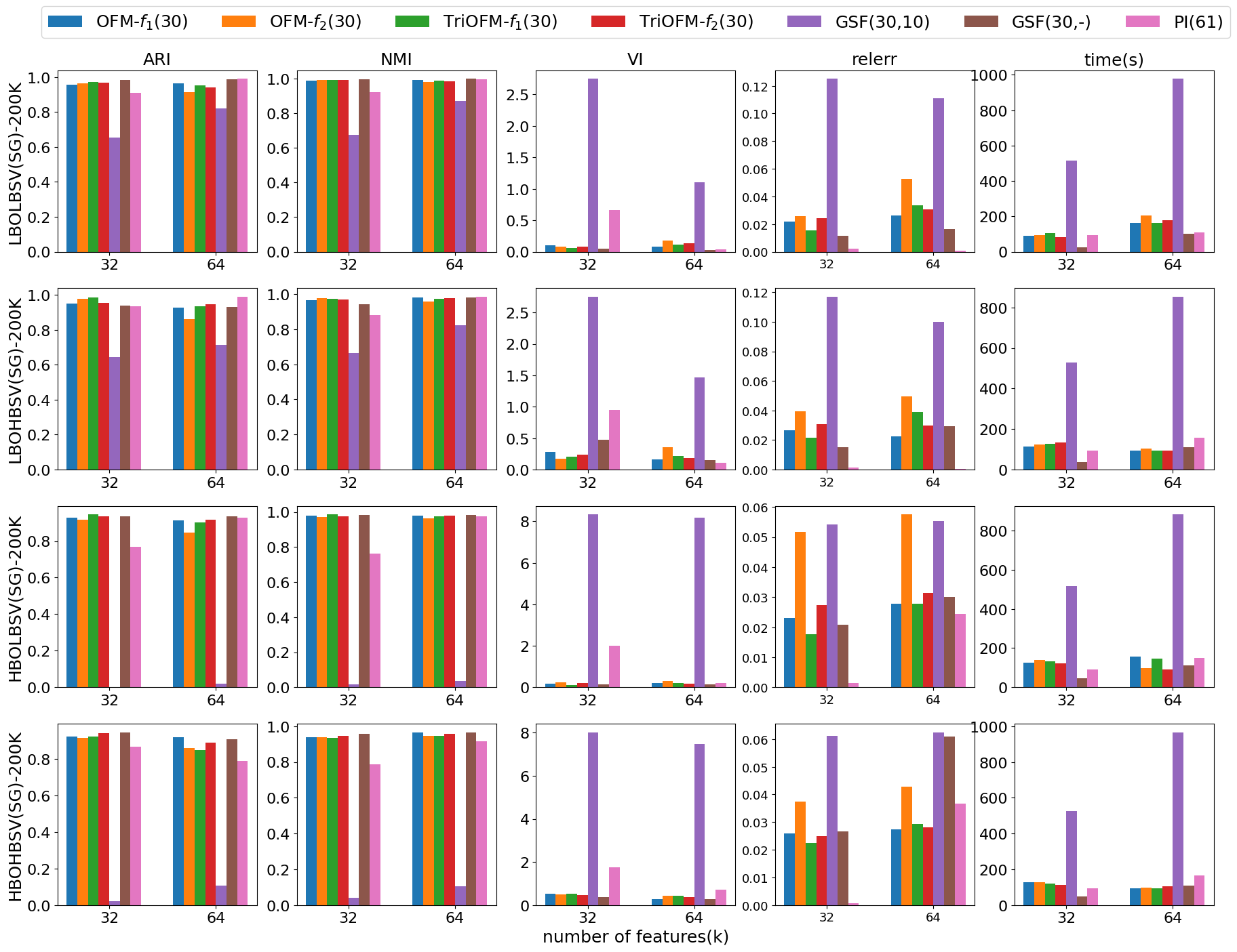
Figure 1: Comparison of the orthogonalization-free methods, GSF, and PI, on clustering static graphs each with $200$ thousand graph nodes.

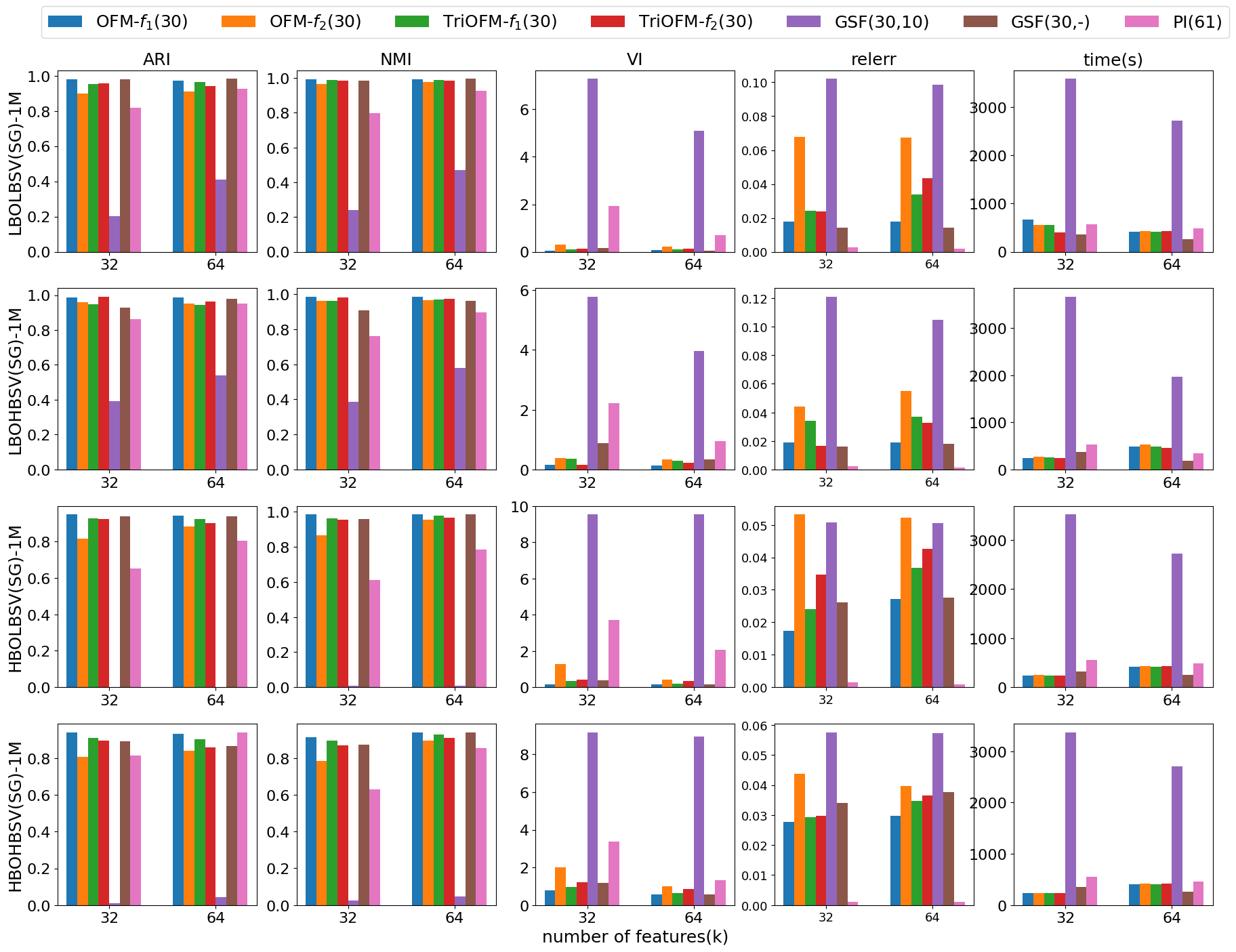
Figure 2: Comparison of the orthogonalization-free methods, GSF, and PI, on clustering static graphs each with $1$ million graph nodes.

2 Orthogonalization-Free Methods

In this section, we describe the sequential orthogonalization-free methods as extensions to Graph Signal Filter. Implementation details will be described in the next section.

2.1 OFM-$f_{1}$ and TriOFM-$f_{1}$

Provided $\mathbf{A}\in\mathbb{R}^{N\times N}$ is the normalized Laplacian of an undirected graph, the ideal low-pass filter of $\mathbf{A}$ is defined as

$$f(\mathbf{A})=\mathbf{U}_{k}h(\mathbf{\Lambda}_{k})\mathbf{U}_{k}^{T}$$ (3)

where $h(\mathbf{\Lambda}_{k})=diag(h(\lambda_{1}),...,h(\lambda_{k}))$, $h(\lambda_{i})=1$ for all $0\leq\lambda_{1}\leq\lambda_{2}\leq...\leq\lambda_{k}\leq 2$, and $\mathbf{U}_{k}$ is a unitary matrix consisting of the corresponding $k$ eigenvectors. J. Paratte and L. Martin [32] prove the following theorem:

Theorem 1.

Let $f$ be an ideal low-pass filter of cutoff frequency $\lambda_{k}$. Let $\mathbf{R}_{k}\in\mathbb{R}^{N\times k}$ be a random matrix formed of entry-wise independent and identically distributed Gaussian random variables with mean $0$ and standard deviation $\frac{1}{k}$. Performing a QR decomposition on the result of the filtering of $\mathbf{R}_{k}$ by $f$ provides the first $k$ eigenvectors of $\mathbf{A}$ altered only by a rotation in $\mathbb{R}^{k}$.

Denote $\mathbf{M}_{k}$ as the filtering of $\mathbf{R}_{k}$, i.e., $\mathbf{M}_{k}=f(\mathbf{A})\mathbf{R}_{k}$. Since it is impractical to obtain the exact eigenvectors $\mathbf{U}_{k}$, it is important to find an approximation of the ideal low-pass filter $f(\mathbf{A})$, which is a piece-wise transformation which maps the smallest $k$ eigenvalues to $1$ and the others to $0$. Chebyshev-type polynomials are one of the most popular methods to approximate such a step function. The Jackson-Chebyshev polynomial approximation is the best suited to approximate the step function inherent in $f(\mathbf{A})$ since it avoids the Gibbs effect of Chebyshev polynomials [32]. The Jackson-Chebyshev polynomial used for filtering is also used in the estimation of the smallest $k$-th eigenvalue $\lambda_{k}$ using the dichotomy and edge count techniques. The aforementioned is how GSF works.

Note that if $f(\mathbf{A})\mathbf{R}_{k}$ provides a good approximation to the eigenspace, so does $-f(\mathbf{A})\mathbf{R}_{k}$. The distance between $\mathbf{A}$ and $-f(\mathbf{A})$ could be measured by $\|A-(-f(\mathbf{A}))\|_{F}^{2}=\|\mathbf{A}+\mathbf{U}_{k}\mathbf{U}_{k}^{T}\|_{F}^{2}$. Hereafter, consider a negative definite matrix $\mathbf{A}=:\mathbf{A}-2\mathbf{I}$. And thus all eigenvalues satisfy $-2\leq\lambda_{1}\leq\lambda_{2}\leq...\leq\lambda_{N}\leq 0$. Denote $\ell$ as the number of negative eigenvalues of a general matrix. Clearly, $\ell=N$ for $\mathbf{A}$. Consider the $f_{1}$ optimization problem

$$\min_{\mathbf{X}\in\mathbb{R}^{N\times k}}f_{1}(\mathbf{X})=\|\mathbf{A}+\mathbf{X}\mathbf{X}^{T}\|_{F}^{2},$$ (4)

where the gradient

$$\nabla f_{1}(\mathbf{X})=4\mathbf{A}\mathbf{X}+4\mathbf{X}\mathbf{X}^{T}\mathbf{X}.$$ (5)

Local minima are computed in an iterative manner

$$\mathbf{X}^{(t+1)}=\mathbf{X}^{(t)}-\alpha\nabla f_{1}(\mathbf{X}^{(t)}),$$ (6)

where $\alpha$ is the step size and superscript $t$ denotes the $t$-th iteration.

It is obvious that $\mathbf{U}_{k}$ is not a local minimum of $f_{1}$ because $\nabla f_{1}(\mathbf{U}_{k})\neq\mathbf{0}$. Hence, it is a natural idea to solve the problem to find a local minimum $\mathbf{X}_{k}$ and employ it as a feature matrix in spectral clustering. Objective $f_{1}$ has no spurious local minimum, and all local minima are global minima. The form of local minima has been proven in [21, 23] and summarized as follows in [11]:

Theorem 2.

All stationary points of $f_{1}$ are of form $\mathbf{X}=\mathbf{U}_{\ell}\sqrt{-\Lambda_{\ell}}\mathbf{S}\mathbf{P}$ and all local minima are of form $\mathbf{X}=\mathbf{U}_{k}\sqrt{-\Lambda_{k}}\mathbf{Q}$, $\mathbf{S}\in\mathbf{R}^{\ell\times\ell}$ is a diagonal matrix with diagonal entries being $0$ or $1$ (at most $k$ $1$’s), $\mathbf{P}\in\mathbb{R}^{\ell\times k}$ and $\mathbf{Q}\in\mathbb{R}^{k\times k}$ are unitary matrices. Further, any local minimum is also a global minimum.

A local minimum $\mathbf{X}=\mathbf{U}_{k}\sqrt{-\Lambda_{k}}\mathbf{Q}$ could take the place of $\mathbf{U}_{k}$ in spectral clustering. Note that a unitary transformation $\mathbf{Q}$ preserves Euclidean distance, which indicates that using $\mathbf{X}$ is equivalent to using $\mathbf{U}_{k}\sqrt{-\Lambda_{k}}$ as a feature matrix for Euclidean distance based K-means clustering. Therefore, OFM-$f_{1}$ approximates the matrix $\mathbf{U}_{k}$ by a local minimum of $f_{1}$ which augments the eigenspace by weights $\sqrt{-\lambda_{1}},...,\sqrt{-\lambda_{k}}$.

Another way of explicitly getting the eigenpairs instead of a point in the eigenspace is to solve the single-column version of $f_{1}$ recursively. For example, we solve the single-column version of $f_{1}$ to get the local minimum $x_{1}=\sqrt{-\lambda_{1}}u_{1}$ where $\lambda_{1}$ and $u_{1}$ are the smallest eigenvalue and eigenvector, respectively. We apply the method to $\mathbf{A}_{2}=\mathbf{A}+x_{1}x_{1}^{T}$ to get $x_{2}=\sqrt{-\lambda_{2}}u_{2}$ where $\lambda_{2}$ and $u_{2}$ are the second smallest eigenvalue and eigenvector, respectively. Note that we have $\nabla f_{1}(x_{2})=4(\mathbf{A}+x_{1}x_{1}^{T})x_{2}+4x_{2}x_{2}^{T}x_{2}=4\mathbf{A}x_{2}+4(x_{1}x_{1}^{T}x_{2}+x_{2}x_{2}^{T}x_{2})$. Similarly, while computing $x_{k}=\sqrt{-\lambda_{k}}u_{k}$ by applying the method to $\mathbf{A}_{k}=\mathbf{A}+\Sigma_{i=1}^{k-1}x_{i}x_{i}^{T}$, we have $\nabla f_{1}(x_{k})=4\mathbf{A}x_{k}+4\Sigma_{i=1}^{k}x_{i}x_{i}^{T}x_{k}$. Based on this observation, Gao et al. [11] propose TriOFM-$f_{1}$ which adopts a new updating direction

$$g_{1}(\mathbf{X})=\mathbf{A}\mathbf{X}+\mathbf{X}triu(\mathbf{X}^{T}\mathbf{X})$$ (7)

instead of the gradient $\nabla f_{1}(\mathbf{X})$. Though $g_{1}$ is not a gradient of any energy function, Gao et al. analyze the fixed point of

$$\mathbf{X}^{(t+1)}=\mathbf{X}^{(t)}-\alpha g_{1}(\mathbf{X}^{(t)}),$$ (8)

in the following theorem [11]:

Theorem 3.

All fixed points of (8) are of form $\mathbf{X}=\mathbf{U}_{\ell}\sqrt{-\Lambda_{\ell}}\mathbf{P}\mathbf{S}$ where $\mathbf{P}\in\mathbb{R}^{\ell\times k}$ is the first $k$ columns of an arbitrary $\ell\times\ell$ permutation matrix, and $\mathbf{S}\in\mathbf{R}^{k\times k}$ is a diagonal matrix with diagonal entries being $0$, $-1$, or $1$. Within these points all stable fixed points are of form $\mathbf{X}=\mathbf{U}_{k}\sqrt{-\Lambda_{k}}\mathbf{D}$, where $\mathbf{D}\in\mathbb{R}^{k\times k}$ is a diagonal matrix with diagonal entries being $1$ or $-1$. Others are unstable fixed points.

Again, using a stable fixed point $\mathbf{X}=\mathbf{U}_{k}\sqrt{-\Lambda_{k}}\mathbf{D}$ is equivalent to using $\mathbf{U}_{k}\sqrt{-\Lambda_{k}}$ as a feature matrix for Euclidean distance based K-means clustering because the transformation $\mathbf{D}$ preserves Euclidean distance. Consequently, OFM-$f_{1}$ and TriOFM-$f_{1}$ essentially construct the same feature space for K-means clustering. Moreover, in the sense of optimizing $f_{1}$, OFM-$f_{1}$ and TriOFM-$f_{1}$ give better approximations compared to GSF because the filtered signals in GSF are not a local minimum of $f_{1}$.

2.2 OFM-$f_{2}$ and TriOFM-$f_{2}$

If we interpret the ideal low-pass filter $f(\mathbf{A})$ in GSF from another perspective, we could extend it to the other orthogonalization-free method. For example, let $k=N$, then $f(\mathbf{A})=\mathbf{U}_{N}\mathbf{U}_{N}^{T}$. Since $\mathbf{A}$ is symmetric, then there is a Cholesky decomposition $\mathbf{A}=\mathbf{L}\mathbf{L}^{T}$. Hence the effectiveness of $f(\mathbf{A})$ could be measured by the sum of the cosine similarity between the columns of $\mathbf{L}$ and $\mathbf{U}_{N}$, i.e.,

$$\|\mathbf{L}^{T}\mathbf{U}_{N}\|_{F}^{2}=tr(\mathbf{U}_{N}^{T}\mathbf{L}\mathbf{L}^{T}\mathbf{U}_{N})=tr(\mathbf{U}_{N}^{T}\mathbf{A}\mathbf{U}_{N})$$ (9)

Obviously, $\mathbf{U}_{N}$ is a local minimum of

$$\min_{\mathbf{X}\in\mathbb{R}^{N\times N},\mathbf{X}^{T}\mathbf{X}=\mathbf{I}_{N}}tr(\mathbf{X}^{T}\mathbf{A}\mathbf{X}),$$ (10)

which is equivalent to the unconstrained optimization problem

$$\min_{\mathbf{X}\in\mathbb{R}^{N\times N}}tr((2\mathbf{I}-\mathbf{X}^{T}\mathbf{X})\mathbf{X}^{T}\mathbf{A}\mathbf{X}).$$ (11)

For general $k$, it becomes the OFM-$f_{2}$ optimization problem

$$\min_{\mathbf{X}\in\mathbb{R}^{N\times k}}f_{2}(\mathbf{X})=:tr((2\mathbf{I}-\mathbf{X}^{T}\mathbf{X})\mathbf{X}^{T}\mathbf{A}\mathbf{X})$$ (12)

with gradient

$$\nabla f_{2}(\mathbf{X})=4\mathbf{A}\mathbf{X}-2\mathbf{X}\mathbf{X}^{T}\mathbf{A}\mathbf{X}-2\mathbf{A}\mathbf{X}\mathbf{X}^{T}\mathbf{X}.$$ (13)

Local minima could be computed in an iterative manner

$$\mathbf{X}^{(t+1)}=\mathbf{X}^{(t)}-\alpha\nabla f_{2}(\mathbf{X}^{(t)}),$$ (14)

where $\alpha$ is the step size and the superscript $t$ denotes the $t$-th iteration.

Note that $\mathbf{U}_{k}$ is a local minimum because $\nabla f_{2}(\mathbf{U}_{k})=\mathbf{0}$. Unlike approximating $\mathbf{U}_{k}$ using a Chebyshev-type polynomial of high degree and expensive evaluation of the $k$-th eigenvalue in GSF, OFM-$f_{2}$ directly evaluates iterations to locate any local minimum, which is a global minimum given the following theory proved by J. Lu and K. Thicke [24].

Theorem 4.

All stationary points of OFM-$f_{2}$ are of form $\mathbf{X}=\mathbf{U}_{N}\mathbf{S}\mathbf{P}$ and all local minima are of form $\mathbf{X}=\mathbf{U}_{k}\mathbf{Q}$, where $S\in\mathbb{R}^{N\times N}$ is a diagonal matrix with diagonal entries being $0$ or $1$ (at most $k$ $1$’s), $\mathbf{P}\in\mathbb{R}^{N\times k}$ and $\mathbf{Q}\in\mathbb{R}^{k\times k}$ are unitary matrices. Further, any local minimum is also a global minimum.

Unlike OFM-$f_{1}$ and TriOFM-$f_{1}$, when used as the feature matrix to feed the Euclidean distance base K-means clustering, the local minimum $\mathbf{X}=\mathbf{U}_{k}\mathbf{Q}$ used in OFM-$f_{2}$ is equal to $\mathbf{U}_{k}$ only altered by a unitary transformation $\mathbf{Q}$ which preserves the Euclidean distance.

Analogous to TriOFM-$f_{1}$, TriOFM-$f_{2}$ [11] employs

$$g_{2}(\mathbf{X})=2\mathbf{A}\mathbf{X}-\mathbf{A}\mathbf{X}triu(\mathbf{X}^{T}\mathbf{X})-\mathbf{X}triu(\mathbf{X}^{T}\mathbf{A}\mathbf{X})$$ (15)

as a new update rule for

$$\mathbf{X}^{(t+1)}=\mathbf{X}^{(t)}-\alpha g_{2}(\mathbf{X}^{(t)}).$$ (16)

The fixed points of (16) are analyzed in the following theorem [11]:

Theorem 5.

All fixed points of (16) are of form $\mathbf{X}=\mathbf{U}_{N}\mathbf{P}\mathbf{S}$ and all stable fixed points are of form $\mathbf{X}=\mathbf{U}_{k}\mathbf{D}$, where $\mathbf{P}\in\mathbb{R}^{\ell\times k}$ is the first $k$ columns of an arbitrary $N\times N$ permutation matrix, $\mathbf{S}\in\mathbf{R}^{k\times k}$ is a diagonal matrix with diagonal entries being $0$, $-1$, or $1$, and $\mathbf{D}\in\mathbf{R}^{k\times k}$ is a diagonal matrix with diagonal entries being $-1$, or $1$.

Therefore, the local minimum constructed by TriOFM-$f_{2}$ lies in the same eigenspace spanned by $\mathbf{U}_{k}$. Though GSF constructs the same feature space as OFM-$f_{2}$ and TriOFM-$f_{2}$, it requires highly accurate $\lambda_{k}$ estimation, which is either impractical or costly. It is guaranteed that OFM-$f_{2}$ and TriOFM-$f_{2}$ highly precisely achieve the desired feature space with optimal stepsizes in each iteration accomplished by line search, which is more practical and reliable.

Note that none of the four optimization methods introduced above acquires orthogonalization which is widely used in ARPACK, LOBPCG, block Chebyshev-Davidson method, PI-based method, and GSF. Though the feature space generated by OFM-$f_{1}$ and TriOFM-$f_{1}$ are weighted eigenspace, numerical results show that it may be as good as the original eigenspace in spectral clustering. In the numerical section, we will demonstrate that these four methods are not merely outperforming GSF but hypothetically equivalent to the ideal GSF, which exploits the exact eigenvalue $\lambda_{k}$ directly.

Figure 3: Comparison of the orthogonalization-free methods, ARPACK, and LOBPCG, on clustering edge-sampling streaming graphs each with $200$ thousand graph nodes.

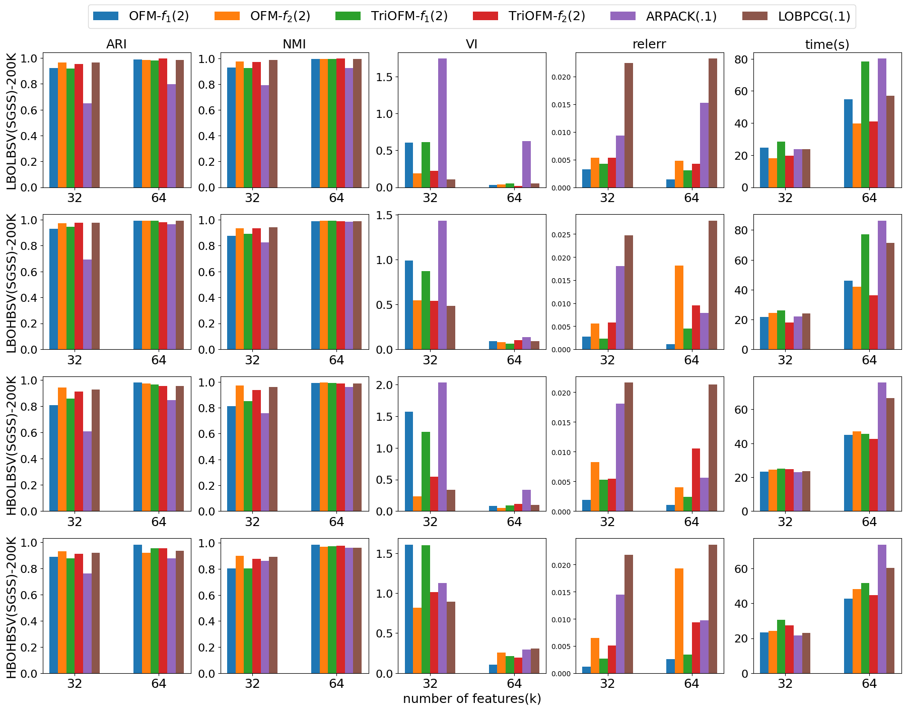
Figure 4: Comparison of the orthogonalization-free methods, ARPACK, and LOBPCG, on clustering snowball-sampling streaming graphs each with $200$ thousand graph nodes.

3 Implementation Details

In this section, we describe how we implement the orthogonalization-free methods, including momentum acceleration, line search for stepsizes, and parallel implementation details of each critical component of the methods.

3.1 Momentum Acceleration

In traditional gradient descent methods, momentum is a widely-used technique to smooth oscillatory trajectory and accelerate convergence [34]. Instead of moving along the gradient direction directly, the momentum method moves along with an accumulation of gradient directions with a discounting parameter $\beta\in(0,1]$, i.e.,

$$\mathbf{V}^{(t)}=\beta g(\mathbf{X}^{(t)})+(1-\beta)\mathbf{V}^{(t-1)},$$ (17)

where $\mathbf{V}^{t}$ denotes the accumulation direction and $g$ is one of $\{\nabla f_{1},g_{1},\nabla f_{2},g_{2}\}$. Then the iteration moves along $\mathbf{V}^{(t)}$ to update $\mathbf{X}^{(t+1)}$ with stepsize $\alpha$, i.e., $\mathbf{X}^{(t+1)}=\mathbf{X}^{(t)}+\alpha\mathbf{V}^{(t)}$. To avoid choosing the momentum parameter $\beta$, we adopt the idea of conjugate gradient (CG) [12], a momentum method with adaptive momentum parameters. F. Corsetti [7] adopts a nonlinear CG in optimizing OFM-$f_{2}$, and Gao et al. [11] adopts a column-wise nonlinear CG, which is an extension to Polak-Reeves CG [33], in TriOFM-$f_{1}$ and TriOMM-$f_{2}$. We adopt the same columnwise nonlinear CG in OFM-$f_{1}$, TriOFM-$f_{1}$, OFM-$f_{2}$, and TriOFM-$f_{2}$ as Algorithm 1, where $\odot$ denotes element-wise multiplication, $\oslash$ denotes element-wise division, and $sumeachcol(\mathbf{G})$ sums each column of $\mathbf{G}$ and returns a column vector.

Algorithm 1 Columnwise CG

1:Input: symmetric matrix $\mathbf{A}$, initial point $\mathbf{X}^{(0)}$, stepsize $\alpha$, maxixum iteration number $t_{max}$

2:$\mathbf{G}^{(0)}=g(\mathbf{X}^{(0)})$

3:$\mathbf{V}^{(0)}=-\mathbf{G}^{(0)}$

4:$\mathbf{X}^{(1)}=\mathbf{X}^{(0)}+\alpha\mathbf{V}^{(0)}$

5:$t=1$

6:while  $t<=t_{max}$ do

7:     $\mathbf{G}^{(t)}=g(\mathbf{X}^{(t)})$

8:     $\mathbf{\beta}^{(t)}=sumeachcol((\mathbf{G}^{(t)}-\mathbf{G}^{(t-1)})\odot\mathbf{G}^{(t)})\oslash sumeachcol(\mathbf{G}^{(t-1)}\odot\mathbf{G}^{(t-1)})$

9:     Compute $\mathbf{V}_{i}^{(t)}=-\mathbf{G}_{i}^{(t)}+\mathbf{\beta}^{(t)}_{i}\mathbf{V}_{i}^{(t-1)}$, for $\forall i$

10:     $\mathbf{X}^{(t+1)}=\mathbf{X}^{(t)}+\alpha\mathbf{V}^{(t)}$

11:     $t=t+1$

12:end while

3.2 Stepsizes

In previous sections, we describe algorithms with a constant stepsize for simplicity. However, choosing a stepsize $\alpha$ is usually tedious, and a terrible choice of $\alpha$ probably impairs the convergence. Thus we adopt an exact line search strategy to determine the optimal stepsizes automatically. We can conduct the exact line search by minimizing quartic polynomials $f_{1}$ and $f_{2}$, or equivalently, calculating the stable points of the derivative cubic polynomials. Taking OFM-$f_{1}$ as an example, the cubic polynomial is

$$\frac{d}{d\alpha}f_{1}(\mathbf{X}+\alpha\mathbf{V}) =tr(\mathbf{V}^{T}\nabla f_{1}(\mathbf{X}+\alpha\mathbf{V}))$$

$$=\alpha^{3}tr((\mathbf{V}^{T}\mathbf{V})^{2})+3\alpha^{2}tr(\mathbf{V}^{T}\mathbf{V}\mathbf{X}^{T}\mathbf{V})$$

$$+\alpha tr(\mathbf{V}^{T}\mathbf{A}\mathbf{V}+(\mathbf{V}^{T}\mathbf{X})^{2}+\mathbf{V}^{T}\mathbf{X}\mathbf{X}^{T}\mathbf{V}+\mathbf{V}^{T}\mathbf{V}\mathbf{X}^{T}\mathbf{X})$$

$$+tr(\mathbf{V}^{T}\mathbf{A}\mathbf{X})+tr(\mathbf{V}^{T}\mathbf{X}\mathbf{X}^{T}\mathbf{X}).$$ (18)

Solving the above equation might result in one, two, or three real roots. There are three different choices of $\alpha$:

• the real root if only one real root exists;

• the real root of single multiplicity if two real roots exist;

• the real root which achieves the minimal function value when three real roots exist.

We could efficiently evaluate a cubic polynomial’s real roots via Cardano’s formula. Though the evaluated stepsize does not work for TriOFM-$f_{1}$, Gao et al. [11] show that we could compute the stepsize for TriOFM-$f_{1}$ in a similar manner by solving $tr(\mathbf{V}_{i}^{T}g_{1}(\mathbf{X}_{i}+\alpha_{i}\mathbf{V}_{i}))=0,\forall i$ instead, which can be expressed as again a cubic polynomial of $\alpha_{i}$:

$$tr(\mathbf{V}_{i}^{T}g_{1}(\mathbf{X}_{i}+\alpha_{i}\mathbf{V}_{i})) =\alpha_{i}^{3}tr(\mathbf{V}_{i}^{T}\mathbf{V}_{i}triu(\mathbf{V}_{i}^{T}\mathbf{V}_{i}))$$

$$+\alpha_{i}^{2}tr(\mathbf{V}_{i}^{T}\mathbf{V}_{i}triu(\mathbf{X}_{i}^{T}\mathbf{V}_{i})+\mathbf{V}_{i}^{T}\mathbf{V}_{i}triu(\mathbf{V}_{i}^{T}\mathbf{X}_{i})+\mathbf{V}_{i}^{T}\mathbf{X}_{i}triu(\mathbf{V}_{i}^{T}\mathbf{V}_{i}))$$

$$+\alpha_{i}tr(\mathbf{V}_{i}^{T}\mathbf{A}\mathbf{V}_{i}+\mathbf{V}_{i}^{T}\mathbf{X}_{i}triu(\mathbf{V}_{i}^{T}\mathbf{X}_{i})+\mathbf{V}_{i}^{T}\mathbf{X}_{i}triu(\mathbf{X}_{i}^{T}\mathbf{V}_{i})+\mathbf{V}_{i}^{T}\mathbf{V}_{i}triu(\mathbf{X}_{i}^{T}\mathbf{X}_{i}))$$

$$+tr(\mathbf{V}_{i}^{T}\mathbf{A}\mathbf{X}_{i}+\mathbf{V}_{i}^{T}\mathbf{X}_{i}triu(\mathbf{X}_{i}^{T}\mathbf{X}_{i})).$$ (19)

Analogous to OFM-$f_{1}$, we compute the stepsizes in OFM-$f_{2}$ by evaluating the roots of

$$\frac{d}{d\alpha}f_{2}(\mathbf{X}+\alpha\mathbf{V}) =tr(\mathbf{V}^{T}\nabla f_{2}(\mathbf{X}+\alpha\mathbf{V}))$$

$$=-4\alpha^{3}tr(\mathbf{V}^{T}\mathbf{V}\mathbf{V}^{T}\mathbf{A}\mathbf{V})-6\alpha^{2}tr(\mathbf{V}^{T}\mathbf{X}\mathbf{V}^{T}\mathbf{A}\mathbf{V}+\mathbf{V}^{T}\mathbf{V}\mathbf{V}^{T}\mathbf{A}\mathbf{X})$$

$$+2\alpha tr(2\mathbf{V}^{T}\mathbf{A}\mathbf{V}-2\mathbf{V}^{T}\mathbf{X}\mathbf{X}^{T}\mathbf{A}\mathbf{V}-2\mathbf{V}^{T}\mathbf{X}\mathbf{V}^{T}\mathbf{A}\mathbf{X}-\mathbf{V}^{T}\mathbf{V}\mathbf{X}^{T}\mathbf{A}\mathbf{X}-\mathbf{X}^{T}\mathbf{X}\mathbf{V}^{T}\mathbf{A}\mathbf{V})$$

$$+2tr(2\mathbf{V}^{T}\mathbf{A}\mathbf{X}-\mathbf{V}^{T}\mathbf{X}\mathbf{X}^{T}\mathbf{A}\mathbf{X}-\mathbf{X}^{T}\mathbf{X}\mathbf{V}^{T}\mathbf{A}\mathbf{X}).$$ (20)

Like TriOFM-$f_{1}$, TriOFM-$f_{2}$ evaluates the stepsizes by solving $tr(\mathbf{V}_{i}^{T}g_{2}(\mathbf{X}_{i}+\alpha_{i}\mathbf{V}_{i}))=0,\forall i$, where

$$tr(\mathbf{V}_{i}^{T}g_{2}(\mathbf{X}_{i}+\alpha_{i}\mathbf{V}_{i})) =-\alpha_{i}^{3}tr(\mathbf{V}_{i}^{T}\mathbf{A}\mathbf{V}_{i}triu(\mathbf{V}_{i}^{T}\mathbf{V}_{i})+\mathbf{V}_{i}^{T}\mathbf{V}_{i}triu(\mathbf{V}_{i}^{T}\mathbf{A}\mathbf{V}_{i}))$$

$$-\alpha_{i}^{2}tr(\mathbf{V}_{i}^{T}\mathbf{A}\mathbf{X}_{i}triu(\mathbf{V}_{i}^{T}\mathbf{V}_{i})+\mathbf{V}_{i}^{T}\mathbf{A}\mathbf{V}_{i}triu(\mathbf{X}_{i}^{T}\mathbf{V}_{i})+\mathbf{V}_{i}^{T}\mathbf{A}\mathbf{V}_{i}triu(\mathbf{V}_{i}^{T}\mathbf{X}_{i})$$

$$+\mathbf{V}_{i}^{T}\mathbf{X}_{i}triu(\mathbf{V}_{i}^{T}\mathbf{A}\mathbf{V}_{i})+\mathbf{V}_{i}^{T}\mathbf{V}_{i}triu(\mathbf{X}_{i}^{T}\mathbf{A}\mathbf{V}_{i})+\mathbf{V}_{i}^{T}\mathbf{V}_{i}triu(\mathbf{V}_{i}^{T}\mathbf{A}\mathbf{X}_{i}))$$

$$+\alpha_{i}tr(2\mathbf{V}_{i}^{T}\mathbf{A}\mathbf{V}_{i}-\mathbf{V}_{i}^{T}\mathbf{A}\mathbf{X}_{i}triu(\mathbf{X}_{i}^{T}\mathbf{V}_{i})-\mathbf{V}_{i}^{T}\mathbf{A}\mathbf{X}_{i}triu(\mathbf{V}_{i}^{T}\mathbf{X}_{i})$$

$$-\mathbf{V}_{i}^{T}\mathbf{A}\mathbf{V}_{i}triu(\mathbf{X}_{i}^{T}\mathbf{X}_{i})-\mathbf{V}_{i}^{T}\mathbf{X}_{i}triu(\mathbf{X}_{i}^{T}\mathbf{A}\mathbf{V}_{i})$$

$$-\mathbf{V}_{i}^{T}\mathbf{X}_{i}triu(\mathbf{V}_{i}^{T}\mathbf{A}\mathbf{X}_{i})-\mathbf{V}_{i}^{T}\mathbf{V}_{i}triu(\mathbf{X}_{i}^{T}\mathbf{A}\mathbf{X}_{i}))$$

$$+tr(2\mathbf{V}_{i}^{T}\mathbf{A}\mathbf{X}_{i}-\mathbf{V}_{i}^{T}\mathbf{A}\mathbf{X}_{i}triu(\mathbf{X}_{i}^{T}\mathbf{X}_{i})-\mathbf{V}_{i}^{T}\mathbf{X}_{i}triu(\mathbf{X}_{i}^{T}\mathbf{A}\mathbf{X}_{i})).$$ (21)

By combining conjugate gradient and exact line search, we summarize the entire framework of the orthogonalization-free method as Algorithm 2.

Algorithm 2 Orthogonalization-free algorithm framework

1:Input: symmetric matrix $\mathbf{A}$, initial point $\mathbf{X}^{(0)}$, stepsize $\alpha$, maximum iteration number $t_{max}$

2:$\mathbf{G}^{(0)}=g(\mathbf{X}^{(0)})$

3:$\mathbf{V}^{(0)}=-\mathbf{G}^{(0)}$

4:$\mathbf{X}^{(1)}=\mathbf{X}^{(0)}+\alpha\mathbf{V}^{(0)}$

5:$t=1$

6:while  $t<t_{max}$ do

7:     $\mathbf{G}^{(t)}=g(\mathbf{X}^{(t)})$

8:     $\mathbf{\beta}^{(t)}=sumeachcol((\mathbf{G}^{(t)}-\mathbf{G}^{(t-1)})\odot\mathbf{G}^{(t)})\oslash sumeachcol(\mathbf{G}^{(t-1)}\odot\mathbf{G}^{(t-1)})$

9:     Compute $\mathbf{V}_{i}^{(t)}=-\mathbf{G}_{i}^{(t)}+\mathbf{\beta}^{(t)}_{i}\mathbf{V}_{i}^{(t-1)}$, for $\forall i$

10:     Evaluate stepsizes $\alpha^{(t)}$ by exact line search

11:     Update $\mathbf{X}_{i}^{(t+1)}=\mathbf{X}_{i}^{(t)}+\mathbf{\alpha}^{(t)}_{i}\mathbf{V}_{i}^{(t)}$, for $\forall i$

12:     $t=t+1$

13:end while

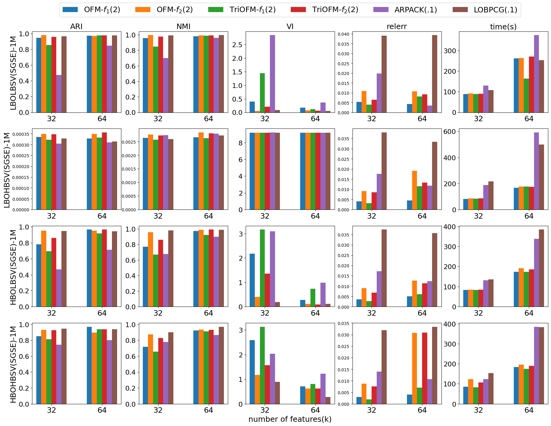
Figure 5: Comparison of the orthogonalization-free methods, ARPACK, and LOBPCG, on clustering edge-sampling streaming graphs each with $1$ million graph nodes.

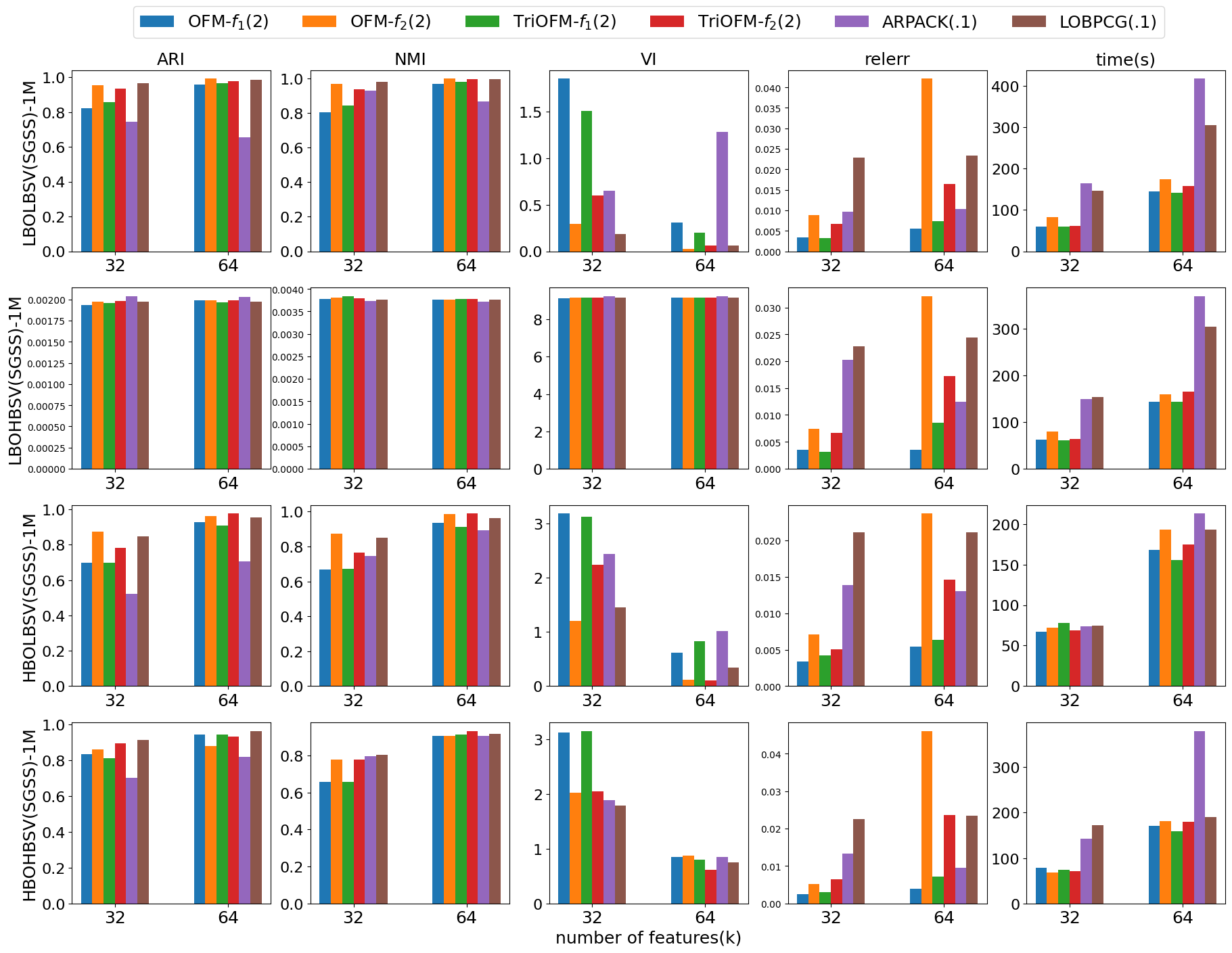
Figure 6: Comparison of the orthogonalization-free methods, ARPACK, and LOBPCG, on clustering snowball-sampling streaming graphs each with $1$ million graph nodes.

Figure 7: We borrow the Figure 1 in [31] as an illustration of A-Stationary 1.5D SpMM $\mathbf{Y}=\mathbf{A}\mathbf{X}$ when the number of processes is $p=9$. The $P(2,1)$ process owns the blocks $\mathbf{Y}[7],\mathbf{X}[5]$, and $\mathbf{A}[2,1]$.

3.3 Parallelization

To handle large-scale graphs, we parallelize and accelerate computation using multiple processes and threads, i.e., hybrid implementation. Multithreading implementation for a single node is straightforward by calling BLAS libraries. In our case, we directly call OpenBLAS library [40] to accelerate dense-dense matrix computation and Intel MKL library [38] for sparse-dense matrix multiplication. Multiprocessing implementation for data distributed among multiple compute nodes requires cautious designs and tremendous efforts, which is the main focus of this section.

The first critical component we need to parallelize is performing distributed sparse matrix times tall-and-skinny matrix (SpMM) computation in the form of

$$\mathbf{Y}=\mathbf{A}\mathbf{X},$$ (22)

where $\mathbf{X}$ and $\mathbf{Y}$ are of size $N\times k$, and $k<<N$. Here matrices $\mathbf{A},\mathbf{X}$ and $\mathbf{Y}$ are distributed among multiple compute nodes. To perform distributed SpMM, we employ the A-Stationary 1.5D algorithm in [36]. Assume a 2D process/node grid $P$ of size $\sqrt{p}\times\sqrt{p}$. The algorithm partitions the sparse matrix $\mathbf{A}$ into a 2D block grid of size $\sqrt{p}\times\sqrt{p}$ and the dense matrices $\mathbf{X}$ and $\mathbf{Y}$ into $p$ row blocks, such that the $(i,j)$-th process $P(i,j)$ owns the $(i,j)$-th block $\mathbf{A}[i,j]$ of $\mathbf{A}$, the $(j\sqrt{p}+i)$-th block $\mathbf{X}[j\sqrt{p}+i]$ of $\mathbf{X}$, and the $(i\sqrt{p}+j)$-th block $\mathbf{Y}[i\sqrt{p}+j]$ of $\mathbf{Y}$. See Figure 7 for an illustration. The algorithm first replicates $\mathbf{X}$ among $\sqrt{p}$ processes in each column of the process grid, such that $P(i,j)$ has $\sqrt{p}$ blocks of $\mathbf{X}$, which are given by $\mathbf{X}[j\sqrt{p}+\ell]$ for $0\leq\ell<\sqrt{p}$. Next, the processes perform the local computation of form $\mathbf{Y}^{j}[i\sqrt{p}+\ell]=\mathbf{A}[i,j]\mathbf{X}[j\sqrt{p}+\ell]$ for $0\leq\ell<\sqrt{p}$ with $\mathbf{Y}^{j}$ denoting the partial dense resulting matrix evaluated by the process at $j$-th column of the grid. In the end, each process sums up the partial dense matrices to get the final result matrix at each process with $\mathbf{Y}[i\sqrt{p}+j]=\Sigma_{\ell=0}^{\sqrt{p}}\mathbf{Y}^{\ell}[i\sqrt{p}+j]$. For more details, please refer to [36]. On average, each process requires $nnz(\mathbf{A})/p+2Nk/\sqrt{p}$ cost to store data, where $nnz(\mathbf{A})$ is the number of nonzeros in $\mathbf{A}$, and $nnz(\mathbf{A})2k/p$ flops to perform local computations.

To analyze communication cost, we assume that it costs $\alpha+\beta w$ time, where $\alpha$ is the latency and $\beta$ is the reciprocal bandwidth, to send a message of size $w$ from one process/node to another [36]. The MPI_Allgather collective is applied to realize the replication among $\sqrt{p}$ processes in each column of the process grid. If implemented with a recursive doubling algorithm, the MPI_Allgather collective at each process takes $\alpha\log p+\beta wp$ cost to gather $w$ words from all processes in the same communicator [4]. Before the replication for each grid column in the A-Stationary 1.5D algorithm, each process has $Nk/p$ words, and thus the respective MPI_Allgather has a cost of $\alpha\log p+\beta Nk/\sqrt{p}$. The MPI_Reduce_scatter collective with a summation operator is adopted to realize the reduction of partial dense matrices among $\sqrt{p}$ processes in a row of the 2D process grid. With a recursive halving implementation, the MPI_Reduce_scatter collective takes $\alpha\log p+\beta w$ cost to collect $w$ words from all process in the same communicator and then scatter $w/p$ words back to each process [4]. In our case, the respective MPI_Reduce_scatter costs $\alpha\log p+\beta Nk/\sqrt{p}$ to reduce and scatter $Nk/\sqrt{p}$ words at each process. Therefore, the total communication cost for an SpMM is

$$2\alpha\log p+\beta\dfrac{2Nk}{\sqrt{p}}.$$ (23)

One may notice that, after evaluating a distributed SpMM, $\mathbf{X}$ and $\mathbf{Y}$ are distributed differently, which induces barriers in further applying $\mathbf{A}$ to $\mathbf{Y}$. To handle this, we transform the process grid first and then implicitly apply the identity matrix to $\mathbf{Y}$ so that $\mathbf{Y}$ and $\mathbf{X}$ share the same distribution. This additional step does not acquire local computation but doubles the communication cost.

Besides SpMM, our algorithms involve plenty of dot-products in the form of $\mathbf{Y}^{T}\mathbf{X}$. Given the partitions of $\mathbf{Y}$ and $\mathbf{X}$, it is natural and efficient to first evaluate the dot-products of the local portions of $\mathbf{X}$ and $\mathbf{Y}$ at each process/node, then sum up all the local products and broadcast the results to every process involved. The local computation takes $2Nk^{2}/p$ flops. We use MPI_Allreduce to realize the summation of local products and broadcast the results. If implemented using a tree algorithm, the MPI_Allreduce collective reduces $w$ words from all processes at a single process and broadcasts the result to all processes in the same communicator, which has $2\alpha\log p+2\beta w\log p$ [4]. Each process has $Nk/p$ words during the computation of $\mathbf{Y}^{T}\mathbf{X}$, thus the communication cost the MPI_Allreduce collective takes is

$$2\alpha\log p+2\beta\dfrac{Nk}{p}\log p.$$ (24)

4 Complexity Analysis

In this section, we analyze each algorithm’s per-iteration time complexity, assuming multi-processing and single-threading implementation. We only analyze the time complexity of the dominating steps $7-11$ in Algorithm 2.

Complexity Analysis of Step 7

The computation $\mathbf{G}^{(t)}=g(\mathbf{X}^{(t)})$ involves an SpMM, multiple dot-products, and rescaling if necessary. Note that $\mathbf{X}^{T}\mathbf{A}\mathbf{X}$ is computed by first performing a SpMM $\mathbf{A}\mathbf{X}$ and then dot-products $\mathbf{X}^{T}(\mathbf{A}\mathbf{X})$. And $\mathbf{X}\mathbf{X}^{T}\mathbf{X}$ is computed by first performing $\mathbf{X}^{T}\mathbf{X}$ and then purely local computation $\mathbf{X}(\mathbf{X}^{T}\mathbf{X})$. Other analogous computations are carried out in the same way as well. The complexity of this step depends on the methods:

• OFM-$f_{1}$: local computation flops: $(nnz(\mathbf{A})2k+4Nk^{2}+Nk)/p$, communication cost: $6\alpha\log p+4Nk\beta/\sqrt{p}+(2Nk\beta\log p)/p$;

• TriOFM-$f_{1}$: local computation flops: $(nnz(\mathbf{A})2k+4Nk^{2}+Nk)/p$, communication cost: $6\alpha\log p+4Nk\beta/\sqrt{p}+(2Nk\beta\log p)/p$;

• OFM-$f_{2}$: local computation flops: $(nnz(\mathbf{A})2k+8Nk^{2}+3Nk)/p$, communication cost: $8\alpha\log p+4Nk\beta/\sqrt{p}+(4Nk\beta\log p)/p$;

• TriOFM-$f_{2}$: local computation flops: $(nnz(\mathbf{A})2k+8Nk^{2}+3Nk)/p$, communication cost: $8\alpha\log p+4Nk\beta/\sqrt{p}+(4Nk\beta\log p)/p$;

Complexity Analysis of Step 8 $\&$ 9

The time complexity of steps 8 and 9 is independent of algorithms. The global summation of each column in step 8 is realized by local addition followed by the MPI_Allreduce collective reducing and broadcasting $k$ words at each process in the same column. Thus, these two steps’ local computation flops and communication costs are $k+7Nk/p$ and $2\alpha\log p+2\beta k\log p$, respectively.

Complexity Analysis of Step 10 $\&$ 11

Given $\alpha^{(t)}$, step 11 only involves local computation, which takes $2Nk/p$ flops. The time complexity of step 10 varies among different algorithms. In general, step 10 involves multiple SpMMs, dot-products, local matrix-matrix multiplication, and trace summation. Some results have been evaluated in the previous steps, e.g., $\mathbf{A}\mathbf{X}$ and $\mathbf{X}^{T}\mathbf{X}$, so we do not need to repeat such redundant computations. According to Section 3.2, some intermediate matrices in the computation are the transpose of some other matrices, and thus plenty of time could be saved by using transposes if available. For example, $\mathbf{V}^{T}\mathbf{A}\mathbf{X}$ is the transpose of $\mathbf{X}^{T}\mathbf{A}\mathbf{V}$, so we only need to compute the latter. Furthermore, we assume finding the roots of a cubic polynomial via Cardano’s formula takes constant $c$ flops. After careful calculation, we provide the complexity of steps 10 and 11 in each algorithm as follows:

• OFM-$f_{1}$: local computation flops: $(nnz(\mathbf{A})2k+8Nk^{2}+2Nk)/p+12k^{3}+4k^{2}+4k+c$, communication cost: $12\alpha\log p+4Nk\beta/\sqrt{p}+(8Nk\beta\log p)/p$;

• TriOFM-$f_{1}$: local computation flops: $(nnz(\mathbf{A})2k+8Nk^{2}+2Nk)/p+16k^{3}+6k^{2}+(4+c)k$, communication cost: $12\alpha\log p+4Nk\beta/\sqrt{p}+(8Nk\beta\log p)/p$;

• OFM-$f_{2}$: local computation flops: $(nnz(\mathbf{A})2k+8Nk^{2}+2Nk)/p+18k^{3}+7k^{2}+4k+c$, communication cost: $12\alpha\log p+4Nk\beta/\sqrt{p}+(8Nk\beta\log p)/p$;

• TriOFM-$f_{2}$: local computation flops: $(nnz(\mathbf{A})2k+8Nk^{2}+2Nk)/p+32k^{3}+14k^{2}+(4+c)k$, communication cost: $12\alpha\log p+4Nk\beta/\sqrt{p}+(8Nk\beta\log p)/p$;

Adding up the complexity of steps 7-11, we get the total per-iteration complexity of every orthogonalization-free algorithm. Table 1 summarizes the asymptotic total complexity, assuming $k<<N$, e.g., $k=\log N$.

Table 2: Properties of matrices used in scalability test. The values under the “load imb.” column present the load imbalance in terms of the sparse matrix elements for 64 compute nodes (i.e., 8 $\times$ 8 2D partition).

Sparse Matrix	N	avg degree	nnz(A)	load imb.
LBOLBSV(SG)-1M	1M	48.4	48.4M	1.15
LBOHBSV(SG)-5M	5M	48.4	242.4M	1.15
LBOHBSV(SG)-20M	20M	48.5	970.1M	1.15
MAWI-Graph-1	18.6M	3.0	56.6M	6.76
Graph500-scale24-ef16	16.8M	31.5	529.4M	5.47

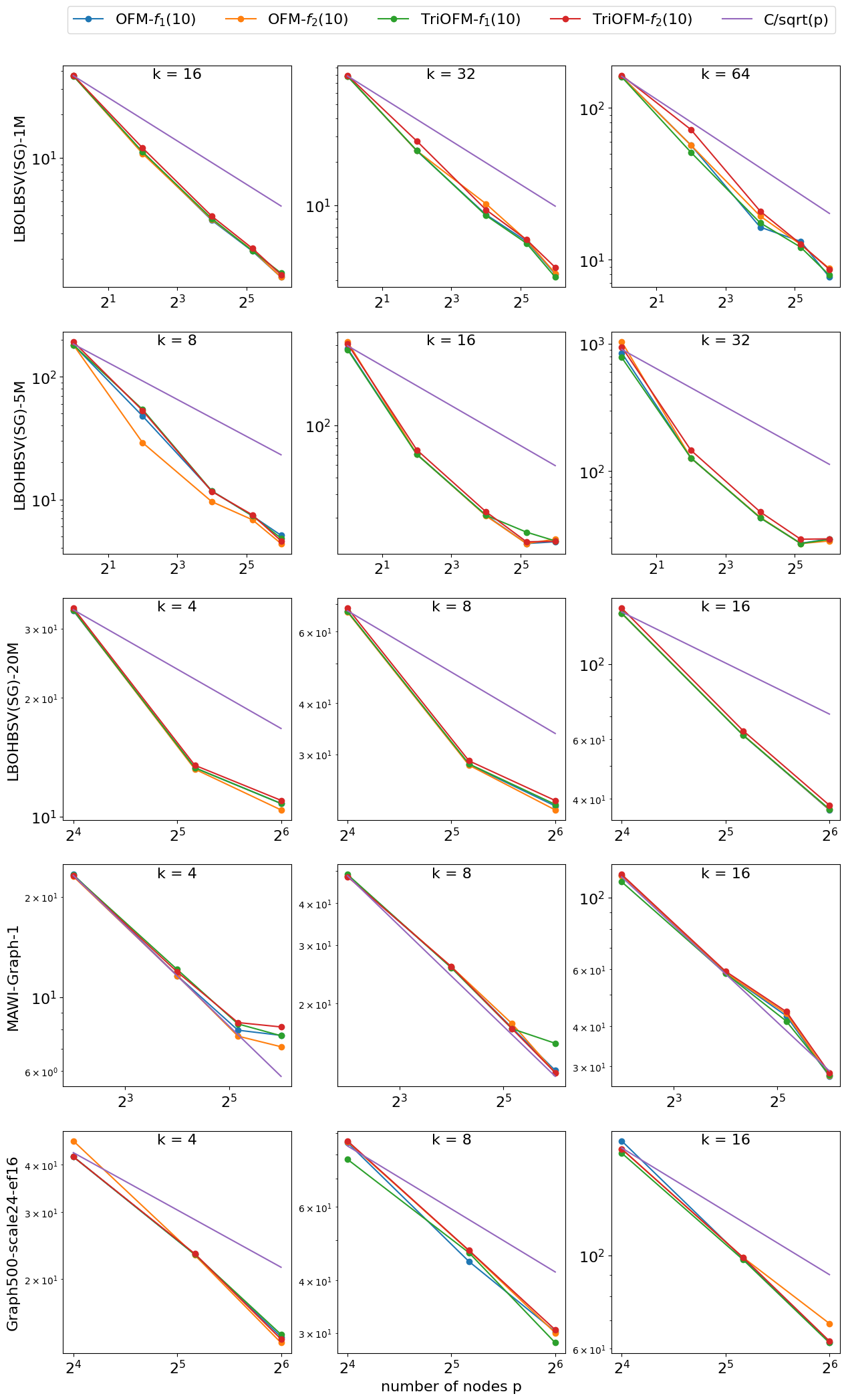
Figure 8: Execution time in seconds that the orthogonalization-free methods use to compute $k$ vectors on five graphs listed in Table 2, against the number of compute nodes. Only one process is used at one node.

5 Numerical Results

In this section, we present the numerical results of three numerical experiments to demonstrate the effectiveness of the orthogonalization-free methods. In the first test, we compare the orthogonalization-free methods with other counterparts who approximate eigenvectors, i.e., PI and GSF, in both efficiency and clustering quality on synthetic static graphs. In the second test, we compare the orthogonalization-free methods with ARPACK and LOBPCG on streaming graphs. The methods used in the first two tests are sequentially implemented, i.e., using one process with one thread. In the third test, we test the scalability of the parallel orthogonalization-free methods. All experiments are conducted on the Zaratan cluster operated by the University of Maryland. The cluster has 360 compute nodes, each with dual 2.45 GHz AMD 7763 64-core CPUs and HDR-100 (100 Gbit) Infiniband interconnects between the nodes, with storage and service nodes connected with full HDR (200 Gbit). The theoretical peak floating-point rate of the cluster is 3.5 Pflops. The code available on Github is written in Julia 1.7.3 using OpenBLAS [40] and Intel MKL [38] libraries for multithreading, and MPI.jl [3] back-ended by OpenMPI [10] library for multiprocessing.

Dataset

The synthetic graphs from Synthetic Data for the Streaming Graph Challenge: Stochastic Block Partition with known truth partitions fall into four categories: Low Block Overlap and Low Block Size Variation (the easiest task) (LBOLBSV), Low Block Overlap and High Block Size Variation (LBOHBSV), High Block Overlap and Low Block Size Variation (HBOLBSV), and High Block Overlap and High Block Size Variation (HBOHBSV). There are three sub-datasets in each category: Static Graphs (SG), Streaming Graphs - Edge Sampling (SGES), and Streaming Graphs - Snowball Sampling (SGSS). Hereafter, we use notations in the form of the category(sub-dataset)-size to represent a synthetic graph from the dataset. For example, LBOLBSV(SG)-1M represents the synthetic graph with 1 million graph nodes in the Static Graphs sub-dataset of the LBOLBSV category. Similarly, LBOLBSV(SGES)-1M represents the synthetic streaming graph with 1 million graph nodes in the Streaming Graphs - Edge Sampling sub-dataset of the LBOLBSV category. The only difference is that streaming graph(s) like LBOLBSV(SGES)-1M indeed consist of ten non-overlapping parts of a graph’s edges.

Evaluation metrics

Since the true partitions are known, we adopt three important external indexes to measure the similarity or difference between the true partitions and the clustering results given by K-means clustering based on the features generated by the orthogonalization-free methods and other competitors. The three crucial indexes are Adjusted Rand Index (ARI) [13], Normalized Mutual Information (NMI) [8], and Variation of Information (VI) [27]. For ARI and NMI, values close to 0 indicate that the two clusterings are primarily independent, while values close to 1 indicate significant agreement. ARI is adjusted against chance, while NMI is not. VI measures the distance between two clusterings and is a simple linear expression involving mutual information. However, unlike mutual information, it is a true metric since it obeys the triangle inequality . For VI, smaller values, which are lower bound by 0, indicate that the two clusterings are closer to one another.

We also record the execution time in seconds for each method to complete. Moreover, if we view all methods as eigensolver, we could measure the relative error (‘relerr’) as well: $\|\mathbf{B}\hat{\mathbf{U}}_{k}-\hat{\mathbf{U}}_{k}\hat{\mathbf{\Lambda}}_{k}\|_{F}/\|\hat{\mathbf{U}}_{k}\hat{\mathbf{\Lambda}}_{k}\|$, where $\mathbf{B}$ is the normalized similarity matrix with transition $2$ on the diagonal, and $\hat{\mathbf{\Lambda}}_{k}$ and $\hat{\mathbf{U}}_{k}$ are the corresponding eigenvalues and eigenvectors. The reason why we define $\mathbf{B}$ in this way is to comply with ARPACK and LOBPCG where we use $\mathbf{B}$ as the input matrix to guarantee positive definiteness. The inpute matrices for the our methods, GSF, and PI are the the normalized similarity matrix with transition $-2$ on the diagonal, the normalized similarity matrix, and the normalized similarity matrix, respectively. Note that the Rayleigh–Ritz method is applied for evaluating $\hat{\mathbf{\Lambda}}_{k}$ and $\hat{\mathbf{U}}_{k}$ for each method.

5.1 Comparisons on Static Graphs

In the first test, we compare the methods which approximate $\mathbf{U}_{k}$, i.e., the four orthogonalization-free methods, GSF in [32], and PI-based method in [22]. To make fair comparisons, we try to maintain the same number of sparse matrix-matrix multiplications for the orthogonalization-free methods and the PI-based method to compare clustering indexes and relative errors of computed eigenvectors. Therefore, we run our methods with $30$ iterations (e.g., ‘OFM-$f_{1}$($30$)’) and the PI-based method ‘PI($61$)’ with $61$ iterations. For GSF, we run a GSF ‘GSF($30,10$)’ with a Jackson-Chebyshev polynomial of $30$ degree and $10$ iterations to estimate the $k$-th eigenvalue, as well as an ideal GSF ‘GSF($30,-$)’ with the same Jackson-Chebyshev polynomial but with the exact smallest $k$-th eigenvalue.

Figures 1 and 2 summarize the comparison results, from where we can observe: 1) the orthogonalization-free methods and the PI-based method significantly outperform GSF in terms of clustering quality, execution time, and relative errors; 2) in terms of clustering quality, the orthogonalization-free methods are as good as the ideal GSF and outperform the PI-based method; 3) the four orthogonalization-free methods have similar performance.

5.2 Comparisons on Streaming Graphs

In the second test, we compare the four orthogonalization-free methods, ARPACK, and LOBPCG on streaming graphs. Since the edges of each graph are divided into ten disjoint parts coming in a streaming manner, in each stage, we add the coming part with the previous parts to build the current sub-graph and utilize the computed features for the previous sub-graph as the initial guess to the iterative methods for evaluating the features for the current sub-graph. Since ARPACK merely utilizes a one-dimensional starting vector, we set the starting vector to the computed eigenvector associated with the smallest eigenvalue if available. LOBPCG usually runs with multigrid preconditioning, which varies from different sub-graphs in the streaming graph scenarios and results in expensive computation costs. Therefore, we run LOBPCG with the identity matrix as a preconditioner in every stage for every sub-graph. The input matrix to ARPACK and LOBPCG is the normalized Laplacian matrix with transition $2$ on the diagonals to ensure positive definiteness. Note that both GSF and PI-based methods require random signals as inputs so that they cannot take advantage of a good initial guess, which consequently indicates that they are not competitive in streaming graphs scenarios.

To make fair comparisons, we maintain the same level of relative errors (i.e., tolerance $0.1$) of computed eigenvectors while comparing clustering quality. We run ARPACK and LOBPCG with prefixed tolerance $0.1$ and the orthogonalization-free methods with $2$ iteration in each stage. The maximum iterations are set to be $200$ for both ARPACK and LOBPCG. Figures 3, 4, 5, and 6 summarize the comparison results on streaming graphs with 200 thousand and 1 million graph nodes, from where we could observe: 1) the orthogonalization-free methods and LOBPCG outperform ARPACK in terms of clustering quality and computation cost; 2) OFM-$f_{2}$ and TriOFM-$f_{2}$ outperform OFM-$f_{1}$ and TriOFM-$f_{1}$ on clustering quality; 3) though OFM-$f_{2}$, TriOFM-$f_{2}$, and LOBPCG achieve similar clustering quality, LOBPCG tends to be more expensive. Nonetheless, due to the use of locking techniques with orthogonalization, ARPACK, and LOBPCG have a practical advantage that the orthogonalization-free methods, GSF and PI, do not have: being able to control the approximation accuracy in advance of computation. Naive locking techniques may be applied to TriOFM-$f_{1}$ and TriOFM-$f_{2}$ [11], which is not considered in this paper.

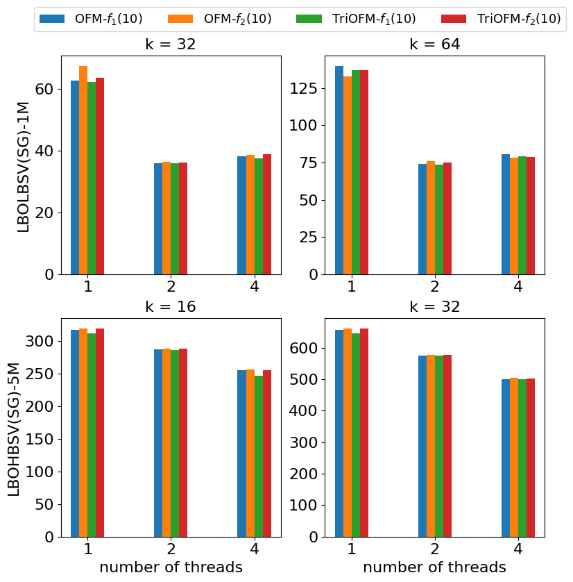
Figure 9: Execution time in seconds that the orthogonalization-free methods use to compute $k$ vectors on LBOLBSV(SG)-1M and LBOHBSV(SG)-5M, against the number of threads used in a process. Only one process is used.

5.3 Scalability

In the third test, we test the scalability of our multiprocessing and multithreading implementation of the four orthogonalization-free methods. We conduct the test on five graphs, including three from the Graph Challenge dataset, i.e., LBOLBSV(SG)-1M, LBOHBSV(SG)-5M, and LBOHBSV(SG)-20M, traffic data from the MAWI Project [6] (MAWI-Graph-1), and synthetic graph data generated using the scalable Graph500 Kronecker generator [15] (Graph500-scale24-ef16). Various properties of these matrices used in the test are presented in Table 2. Load imbalance is defined as the ratio of the maximum number of nonzeros assigned to a process to the average number of nonzeros in each process:

$$\dfrac{p*\max_{i,j}nnz(\mathbf{A}[i,j])}{nnz(\mathbf{A})}.$$ (25)

Figure 8 showcases the execution time of each method on multiple graphs against the number of compute nodes and demonstrates the $1/\sqrt{p}$ speedup where $p$ is the number of compute nodes. Note that, in the experiment, there is only one process with one thread at each node. Figure 9 presents the execution time against the number of threads in an experiment with only one process. One may observe that the speedup drops quickly as the number of threads increases. We believe this is a common phenomenon in multithreading computation, especially when the computation burden is relatively small. The multithreading implementation entirely relies on the OpenBLAS and Intel MKL libraries.

6 Conclusions

We propose four orthogonalization-free methods for dimensionality reduction in spectral clustering by minimizing two objective functions. In contrast to ARPACK, LOBPCG, the block Chebyshev-Davidson method, GSF, and PI, our methods do not require orthogonalization which is known as not scalable in parallel computation, but still construct adequate feature space with theoretical guarantees. We theoretically view the proposed methods as extensions to GSF and numerically hypothesize that they may be equivalent in clustering quality to the ideal GSF, which exploits the exact eigenvalue $\lambda_{k}$ directly without expensive eigenvalue estimation. Numerical results demonstrate that the proposed methods outperform PI-based methods and significantly outperform GSF in clustering quality and computation cost. These methods also show advantages in computation cost in the streaming graph scenarios by utilizing previously computed features as initial vectors when compared to ARPACK and LOBPCG. More specifically, the proposed methods, especially OFM-$f_{2}$ and TriOFM-$f_{2}$, outperform ARPACK in clustering quality and computation cost, and also outperform LOBPCG in computation cost. One drawback of these methods, like GSF and PI, is that we may not know the number of iterations needed in advance. One of the remedies to this is to adopt locking techniques which may acquire orthogonalization steps. Naive locking techniques may be applied to TriOFM-$f_{1}$ and TriOFM-$f_{2}$ [11], which could be a future direction. Besides sequential implementation, we present multithreading implementation via the OpenBLAS and Intel MKL libraries and multiprocessing implementation via the OpenMPI library. Numerical results have demonstrated the effectiveness and scalability of our parallel implementation.

7 Acknowledgments

We thank Aleksey Urmanov from Oracle Lab at Oracle Corporation for the helpful discussion and comments. We thank Oracle Labs, Oracle Corporation, Austin, TX, for providing funding that supported research in the area of scalable spectral clustering and distributed eigensolvers.

References

- [1] M. Belkin and P. Niyogi. Laplacian eigenmaps for dimensionality reduction and data representation. Neural computation, 15(6):1373–1396, 2003.
- [2] C. Boutsidis, P. Kambadur, and A. Gittens. Spectral clustering via the power method-provably. In International conference on machine learning, pages 40–48. PMLR, 2015.
- [3] S. Byrne, L. C. Wilcox, and V. Churavy. Mpi. jl: Julia bindings for the message passing interface. In Proceedings of the JuliaCon Conferences, volume 1, page 68, 2021.
- [4] E. Chan, M. Heimlich, A. Purkayastha, and R. Van De Geijn. Collective communication: theory, practice, and experience. Concurrency and Computation: Practice and Experience, 19(13):1749–1783, 2007.
- [5] W.-Y. Chen, Y. Song, H. Bai, C.-J. Lin, and E. Y. Chang. Parallel spectral clustering in distributed systems. IEEE transactions on pattern analysis and machine intelligence, 33(3):568–586, 2010.
- [6] K. Cho, K. Mitsuya, and A. Kato. Traffic data repository at the WIDE project. In 2000 USENIX Annual Technical Conference (USENIX ATC 00), 2000.
- [7] F. Corsetti. The orbital minimization method for electronic structure calculations with finite-range atomic basis sets. Computer Physics Communications, 185(3):873–883, 2014.
- [8] L. Danon, A. Diaz-Guilera, J. Duch, and A. Arenas. Comparing community structure identification. Journal of statistical mechanics: Theory and experiment, 2005(09):P09008, 2005.
- [9] E. Di Napoli, E. Polizzi, and Y. Saad. Efficient estimation of eigenvalue counts in an interval. Numerical Linear Algebra with Applications, 23(4):674–692, 2016.
- [10] E. Gabriel, G. E. Fagg, G. Bosilca, T. Angskun, J. J. Dongarra, J. M. Squyres, V. Sahay, P. Kambadur, B. Barrett, A. Lumsdaine, et al. Open mpi: Goals, concept, and design of a next generation mpi implementation. In European Parallel Virtual Machine/Message Passing Interface Users’ Group Meeting, pages 97–104. Springer, 2004.
- [11] W. Gao, Y. Li, and B. Lu. Triangularized orthogonalization-free method for solving extreme eigenvalue problems. Journal of Scientific Computing, 93(3):1–28, 2022.
- [12] G. H. Golub and C. F. Van Loan. Matrix computations. JHU press, 2013.
- [13] L. Hubert and P. Arabie. Comparing partitions. Journal of classification, 2:193–218, 1985.
- [14] Z. Huo, G. Mei, G. Casolla, and F. Giampaolo. Designing an efficient parallel spectral clustering algorithm on multi-core processors in julia. Journal of Parallel and Distributed Computing, 138:211–221, 2020.
- [15] J. Kepner, S. Samsi, W. Arcand, D. Bestor, B. Bergeron, T. Davis, V. Gadepally, M. Houle, M. Hubbell, H. Jananthan, et al. Design, generation, and validation of extreme scale power-law graphs. arXiv preprint arXiv:1803.01281, 2018.
- [16] A. V. Knyazev. Toward the optimal preconditioned eigensolver: Locally optimal block preconditioned conjugate gradient method. SIAM journal on scientific computing, 23(2):517–541, 2001.
- [17] R. B. Lehoucq, D. C. Sorensen, and C. Yang. ARPACK users’ guide: solution of large-scale eigenvalue problems with implicitly restarted Arnoldi methods. SIAM, 1998.
- [18] Q. Lei, K. Zhong, and I. S. Dhillon. Coordinate-wise power method. Advances in Neural Information Processing Systems, 29, 2016.
- [19] T. Li, Y. Zhang, H. Liu, G. Xue, and L. Liu. Fast compressive spectral clustering for large-scale sparse graph. IEEE Transactions on Big Data, 8(1):193–202, 2019.
- [20] Y. Li and J. Lu. Optimal orbital selection for full configuration interaction (optorbfci): Pursuing the basis set limit under a budget. Journal of Chemical Theory and Computation, 16(10):6207–6221, 2020.
- [21] Y. Li, J. Lu, and Z. Wang. Coordinatewise descent methods for leading eigenvalue problem. SIAM Journal on Scientific Computing, 41(4):A2681–A2716, 2019.
- [22] F. Lin and W. W. Cohen. Power iteration clustering. 2010.
- [23] X. Liu, Z. Wen, and Y. Zhang. An efficient gauss–newton algorithm for symmetric low-rank product matrix approximations. SIAM Journal on Optimization, 25(3):1571–1608, 2015.
- [24] J. Lu and K. Thicke. Orbital minimization method with l1 regularization. Journal of Computational Physics, 336:87–103, 2017.
- [25] J. Lu and H. Yang. Preconditioning orbital minimization method for planewave discretization. Multiscale Modeling & Simulation, 15(1):254–273, 2017.
- [26] F. Mauri, G. Galli, and R. Car. Orbital formulation for electronic-structure calculations with linear system-size scaling. Physical Review B, 47(15):9973, 1993.
- [27] M. Meilă. Comparing clusterings by the variation of information. In Learning Theory and Kernel Machines: 16th Annual Conference on Learning Theory and 7th Kernel Workshop, COLT/Kernel 2003, Washington, DC, USA, August 24-27, 2003. Proceedings, pages 173–187. Springer, 2003.
- [28] M. Naumov and T. Moon. Parallel spectral graph partitioning. NVIDIA, Santa Clara, CA, USA, Tech. Rep., NVR-2016-001, 2016.
- [29] A. Ng, M. Jordan, and Y. Weiss. On spectral clustering: Analysis and an algorithm. Advances in neural information processing systems, 14, 2001.
- [30] P. Ordejón, D. A. Drabold, M. P. Grumbach, and R. M. Martin. Unconstrained minimization approach for electronic computations that scales linearly with system size. Physical Review B, 48(19):14646, 1993.
- [31] Q. Pang and H. Yang. A distributed block chebyshev-davidson algorithm for parallel spectral clustering, 2022.
- [32] J. Paratte and L. Martin. Fast eigenspace approximation using random signals. arXiv preprint arXiv:1611.00938, 2016.
- [33] E. Polak and G. Ribiere. Note sur la convergence de méthodes de directions conjuguées. Revue française d’informatique et de recherche opérationnelle. Série rouge, 3(16):35–43, 1969.
- [34] N. Qian. On the momentum term in gradient descent learning algorithms. Neural networks, 12(1):145–151, 1999.
- [35] D. Ramasamy and U. Madhow. Compressive spectral embedding: sidestepping the svd. Advances in neural information processing systems, 28, 2015.
- [36] O. Selvitopi, B. Brock, I. Nisa, A. Tripathy, K. Yelick, and A. Buluç. Distributed-memory parallel algorithms for sparse times tall-skinny-dense matrix multiplication. In Proceedings of the ACM International Conference on Supercomputing, pages 431–442, 2021.
- [37] N. Tremblay, G. Puy, R. Gribonval, and P. Vandergheynst. Compressive spectral clustering. In International conference on machine learning, pages 1002–1011. PMLR, 2016.
- [38] E. Wang, Q. Zhang, B. Shen, G. Zhang, X. Lu, Q. Wu, Y. Wang, E. Wang, Q. Zhang, B. Shen, et al. Intel math kernel library. High-Performance Computing on the Intel® Xeon Phi™: How to Fully Exploit MIC Architectures, pages 167–188, 2014.
- [39] Y. Weiss. Segmentation using eigenvectors: a unifying view. In Proceedings of the seventh IEEE international conference on computer vision, volume 2, pages 975–982. IEEE, 1999.
- [40] Z. Xianyi, W. Qian, and Z. Yunquan. Model-driven level 3 blas performance optimization on loongson 3a processor. In 2012 IEEE 18th international conference on parallel and distributed systems, pages 684–691. IEEE, 2012.
- [41] W. Yan, U. Brahmakshatriya, Y. Xue, M. Gilder, and B. Wise. p-pic: parallel power iteration clustering for big data. Journal of Parallel and Distributed computing, 73(3):352–359, 2013.
- [42] W. Ye, S. Goebl, C. Plant, and C. Böhm. Fuse: Full spectral clustering. In Proceedings of the 22nd ACM SIGKDD International Conference on Knowledge Discovery and Data Mining, pages 1985–1994, 2016.
- [43] L. Zelnik-Manor and P. Perona. Self-tuning spectral clustering. Advances in neural information processing systems, 17, 2004.