Appliance Detection Using Very Low-Frequency Smart Meter Time Series

Abstract.

In recent years, smart meters have been widely adopted by electricity suppliers to improve the management of the smart grid system. These meters usually collect energy consumption data at a very low frequency (every 30min), enabling utilities to bill customers more accurately. To provide more personalized recommendations, the next step is to detect the appliances owned by customers, which is a challenging problem, due to the very-low meter reading frequency. Even though the appliance detection problem can be cast as a time series classification problem, with many such classifiers having been proposed in the literature, no study has applied and compared them on this specific problem. This paper presents an in-depth evaluation and comparison of state-of-the-art time series classifiers applied to detecting the presence/absence of diverse appliances in very low-frequency smart meter data. We report results with five real datasets. We first study the impact of the detection quality of 13 different appliances using 30min sampled data, and we subsequently propose an analysis of the possible detection performance gain by using a higher meter reading frequency. The results indicate that the performance of current time series classifiers varies significantly. Some of them, namely deep learning-based classifiers, provide promising results in terms of accuracy (especially for certain appliances), even using 30min sampled data, and are scalable to the large smart meter time series collections of energy consumption data currently available to electricity suppliers. This paper appeared in ACM e-Energy 2023.

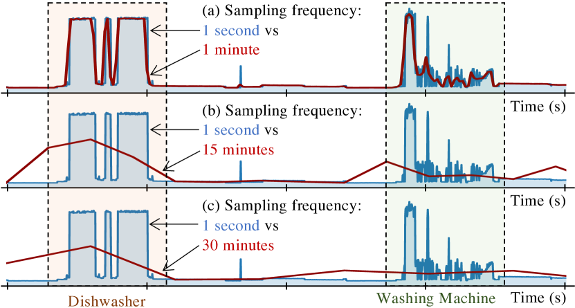
Figure 1. Comparisons of load curves containing a dishwasher and a washing machine at different sampling frequencies (1 second vs 1, 15, and 30min)

1. Introduction

The energy sector is undergoing significant changes, primarily driven by the need for a more sustainable and secure energy supply. One way to better manage our consumption is to understand it better. In the last decade, electricity suppliers have installed millions of smart meters worldwide to improve their ability to manage the electrical grid (Chren et al., 2016; Milam and Kumar Venayagamoorthy, 2014). These meters record detailed time-stamped data on electricity consumption, allowing both individual customers and businesses to better understand and rationalize their consumption (Barai et al., 2015). These data are also valuable for suppliers, as they can help them anticipate energy demand more accurately. Overall, the widespread adoption of smart meters plays a crucial role in transitioning toward a more sustainable and efficient energy system.

We note that it has become essential for electricity suppliers to know which electrical appliances their customers own. This knowledge allows suppliers to better segment their customer base (Allcott, 2011), and therefore to propose personalized offers and services that increase the customer satisfaction and retention. Furthermore, they can help customers rationalize their electricity consumption, therefore contributing to the energy transition. One way to gather this information is by asking customers directly through a consumption questionnaire. However, this method can be a significant investment in terms of time and resources, which customers may not accept, and is also prone to errors. Therefore, electricity suppliers need to find more efficient and non-intrusive ways of gathering this information, such as using advanced data analytics techniques to detect the appliances directly through the collected smart meters data (Hart, 1992).

Appliance detection has become a significant area of research, with various techniques employed to detect the presence of devices (Liu et al., 2021; Rossier et al., 2017). This problem is closely related to Non-Intrusive Load Monitoring (NILM), which aims to identify the power consumption, pattern, or on/off state activation of individual appliances using only the total consumption series (Kaselimi et al., 2022). While detecting an appliance can be seen as a step in NILM-based methods (Qu et al., 2023; Aslan and Nur Zurel, 2022; Tabatabaei et al., 2017; Paradiso et al., 2013; Kahl et al., 2017, 2022; Laviron et al., 2021), and diverse approaches have been proposed in the literature (Qu et al., 2023; Aslan and Nur Zurel, 2022; Tabatabaei et al., 2017; Paradiso et al., 2013; Kahl et al., 2017, 2022; Laviron et al., 2021), they differ from our objective. Indeed, these studies essentially focus on detecting when a specific appliance is ”ON” rather than if a household owns a specific appliance, and the presence of a specific appliance is in several cases already known before applying these approaches. Moreover, the majority of the NILM studies rely on data sampled at $\geq$1Hz, and consequently use signature-based methods (Liu et al., 2021; Rossier et al., 2017) that require either knowledge about how each appliance operates, or training on their individual power consumption. Nonetheless, most existing smart meter installations record consumption at a very low sampling frequency: once every 10 to 60 minutes (in some cases at an even lower frequency). This results in signals where the unique appliance pattern information has been smoothed-out, or lost. Figure 1 illustrates this loss of information. We observe that the dishwasher (shown on the left) and washing machine (shown on the right) signatures become increasingly hard to distinguish from one another as the sampling frequency drops. Therefore, it becomes infeasible to accurately detect appliances using signature-based methods for the sampling frequencies actually used in practice.

In this paper, we propose a benchmark of diverse state-of-the-art classification methods for the problem of appliance detection in very low-frequency electrical consumption time series. We conduct our experimental evaluation on five real smart meter datasets using different time series classifiers. We first focus on detecting appliances in very low-sampled smart meters data (30min level), as it is nowadays one of the standard sampling rates adopted by electricity suppliers. We then provide an in-depth analysis of the increasing detection quality using higher frequency smart meter readings: 15min, 10min, and 1 min. To our knowledge, this is the first study to perform an exhaustive comparison of 11 state-of-the-art methods on five diverse real datasets with 13 different types of appliances, for multiple sampling frequencies. The experimental evaluation demonstrates that current time series classifiers can accurately detect several appliances, even at the 30min resolution. Specifically, deep learning techniques are the most accurate and scalable when applied to large smart meter datasets. Moreover, we demonstrate that setting the smart meter reading frequency to 1min can greatly enhance appliance detection using time series classifiers.

Our contributions are summarized as follows.

• We describe a framework for comparing the performance of different time series classification methods for the appliance detection problem, and make this framework publicly available: https://github.com/adrienpetralia/ApplianceDetectionBenchmark

• We perform an extensive experimental evaluation using 5 diverse real datasets and 11 time series classifiers, including both traditional machine learning, as well as deep learning methods.

• We report the results of our comparison, which demonstrate that (i) current time series classifiers can only detect certain appliances at the 30min resolution; (ii) deep learning classifiers are the most accurate and scalable solution; and (iii) electricity suppliers should target a minimum smart meter reading frequency of 15min.

• The findings of this study can help electricity suppliers make informed decisions regarding the characteristics of future smart meter deployments. Moreover, these findings point to interesting (and still challenging) open research directions in the context of electricity consumption time series analysis, and appliance detection in particular.

2. Background and related work

2.1. Smart Meter Data

An electrical consumption load curve is defined as a univariate time series $\mathcal{X}=(\boldsymbol{x}_{1},...,\boldsymbol{x}_{T})$ of ordered elements $\boldsymbol{x}_{j}\in\mathbb{R}_{+}^{1}$ following $(i_{1},...,i_{T})$ time consumption indexes (i.e., timestamps). The sampling frequency is defined as the time difference between two records index $\Delta_{t}\coloneqq i_{j}-i_{j-1}$. Each element $\boldsymbol{x}_{j}$, usually given in Watt, indicates either the actual power at time $i_{j}$ or the average electric power called during the interval time $\Delta_{t}$. The value can also be given in Watt-hour. In the literature, the definition of high and low-frequency smart meters data can differ (Huber et al., 2021). In this study, we refer to high-frequency data sampled at less than 1 second and low-frequency data sampled between 1 second and 1min. Data sampled above 1min refers to very low-frequency smart meter data.

[Individual appliance load curve] By monitoring electric devices with individual meters, we can obtain the consumption load curve of each individual appliance in a household. However, instrumenting every appliance in the house is prohibitively expensive.

[Aggregate load curve] The main consumption power of a house is usually recorded by a smart meter device located on the electrical meter of the household. This aggregate signal is the addition of the power consumption of all individual appliances in the household.

2.2. Non-Intrusive Load Monitoring (NILM) and Appliance Detection

Non-Intrusive Load Monitoring (NILM) (Hart, 1992), also called load disaggregation, relies on identifying the individual power consumption, pattern, or on/off state activation of individual appliances using only the total aggregated load curve (Kaselimi et al., 2022). NILM was initially approached as a problem involving linear combinations, with algorithms aiming to estimate the proportion of total power consumption used by distinct active appliances at each time step (Kaselimi et al., 2022). Early research on this topic employed combinatorial optimization techniques (Kaselimi et al., 2022). Later, Hidden Markov Models became the dominant approach, and in the last few years, deep learning models have been the reference to perform disaggregation (Kelly and Knottenbelt, 2015a; Kaselimi et al., 2022; Huber et al., 2021; Yue et al., 2020; Sykiotis et al., 2022). Furthermore, NILM approaches can be divided into supervised and unsupervised learning, depending on whether they usee labeled data for training the models. Supervised learning involves classifying detected events (appliances being switched on or off) by matching extracted features (Tabatabaei et al., 2017; Paradiso et al., 2013; Liu et al., 2021; Laviron et al., 2021). In contrast, unsupervised NILM methods detect events by analyzing feature similarities, or correlations without using labeled data (Zhao et al., 2016; Hart, 1992).

Since device recognition can be seen as a step of NILM-based methods, different approaches exist in the literature to detect appliances in load curves using high or low-frequency smart meter data (Qu et al., 2023; Aslan and Nur Zurel, 2022; Tabatabaei et al., 2017; Paradiso et al., 2013; Kahl et al., 2017, 2022; Laviron et al., 2021). However, numerous studies using pattern recognition at low frequency require knowledge about how each device operates. Few recent research studies (Kahl et al., 2022; Paradiso et al., 2013; Aslan and Nur Zurel, 2022; Laviron et al., 2021) used time series features, or deep learning representations, to detect events or appliance activation patterns. Despite the promising results demonstrated by these studies using modern machine learning approaches, we note that they are only applied to high-frequency data (i.e., data sampled at a minimum rate of 1 sample per second).

2.2.1. Studies on Very Low-Frequency Data

Most NILM studies use high-frequency smart-meter data (seconds level at maximum), and only very few studies have been conducted using very-low sampling rates (Miyasawa et al., 2019; Zhao et al., 2020; Eibl and Engel, 2015). In (Zhao et al., 2020), the authors suggested three methods to estimate appliance consumption using hourly smart meter data. The first two methods are unsupervised and require knowledge about manufacturer appliance parameters. The third method is a supervised deep learning approach that requires disaggregate appliance load curves for training. In (Eibl and Engel, 2015), the authors proposed a data privacy-oriented study to assess the impact of Smart Meters sampling frequency on the detection of certain electrical appliances. They used an event detection approach as a feature extractor to train a classifier that identifies changes in power consumption. However, the experimental evaluation in this study was rather limited: the authors evaluated the classification performance on a single dataset, and used the same house for both training and testing. Overall, the few NILM studies that used low-frequency data focus on estimating the consumed power of each appliance, rather than detecting which appliances are present in the households.

Few papers in the literature (Albert and Rajagopal, 2013; Deng et al., 2022) try to tackle the problem of detecting the devices owned by a household using very low-frequency sampled data. In (Albert and Rajagopal, 2013), the authors used a Hidden Semi-Markov Model (HSMM) to extract appliance features from power consumption data. These features are then merged with external variables (such as temperature) and serve to train an AdaBoost classifier (Schapire, 2013) to detect the presence of different appliances. In (Deng et al., 2022), the authors proposed a framework that uses a deep learning approach on subsequences of a long consumption load curve to detect the appliances present in the household. A majority vote gives the final device prediction, based on the individual predictions made on every examined subsequence. The study compares their method to (Albert and Rajagopal, 2013), but not to any of the current state-of-the-art time series classifiers. In addition, only one public dataset at one sampling rate was considered.

2.3. Time Series Classification

Time series classification (TSC) (Bagnall et al., 2016; Ismail Fawaz et al., 2019) is an important analysis task across several domains. Many studies have suggested different approaches to solve the TSC problem, ranging from the computation of similarity measures between time series (Cover and Hart, 1967) to the identification of discriminant patterns (Hills et al., 2014). In addition, benchmarks, such as the the UCR archive (Dau et al., 2018), have been proposed, on which exaustive experimental studies have been conducted (Bagnall et al., 2016). We discuss in more detail the current state-of-the-art time series classifiers in Section 3.

3. Problem Definition and Benchmark

3.1. Problem Definition

In this work, we treat the appliance detection problem as a supervised binary classification problem. We aim to identify the presence/absence of a specified appliance’s activation signature in a smart meter data series, independently of the number of activations of this appliance. The presence can be simply defined by the fact that the device is switched ”ON” at least once. Formally, we define the problem as follows:

Definition 3.0 (Appliance Detection Problem).

Given an aggregate smart meter time series $\mathcal{X}\in\mathbb{R}^{T}$, an appliance type $a$, we want to know if appliance $a$ is activated at least once in $\mathcal{X}$ (i.e., was in an ”ON” state, regardless of the time and number of activations).

3.2. Overview of Time Series Classifiers

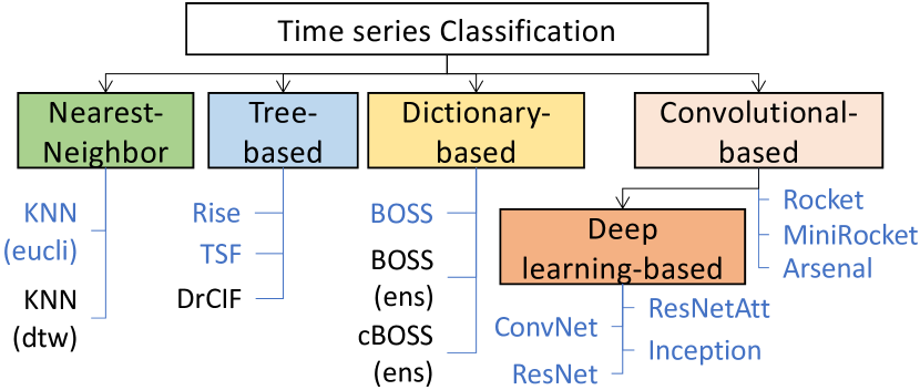
Figure 2. Taxonomy of classifier considered in our benchmark (in blue: classifier used in the experimental evaluation).

We now provide an overview of the different approaches proposed in the literature to solve the TSC problem (refer to Figure 2). The objective is to compare the performance of these methods when applied to the appliance detection problem. Each classifier takes as input for training the univariate consumption time series (i.e., 1D signal) along with the ground-truth labels.

3.2.1. Nearest-Neighbor Classifier

$K$-Nearest-Neighbor ($K$-NN) classifiers are the most simple and intuitive classifiers, based on the notion of time series similarity. Following a chosen distance measure, each new instance is classified by getting assigned the same label as the majority label of the $K$ closest samples in the training set ($K=1$ in our experiments, i.e., we use 1-NN classifiers). The most popular distance measure is Euclidean distance, which allows comparing two instances point to point. However, this distance does not consider the possible distortions on the temporal axis. Dynamic Time Warping (DTW) (Sakoe and Chiba, 1978) is a distance measure to compute the similarity between two time series, where relevant patterns may evolve at different speeds. DTW suffers from a high computational cost, which makes it challenging to apply on large datasets.

3.2.2. Tree Based Classifier

Tree-based classifiers, like Random Forest (Breiman, 2001), have exhibited promising results in classification tasks.

[Time Series Forest] TSF (Deng et al., 2013) is a random forest-based classifier that uses as input features extracted from randomly sampled intervals of the raw data series. The algorithm first selects a number $r$ of intervals with a random start position and length; then, from each interval, three simple features are extracted: the mean, the standard deviation, and the slope. Finally, the $3r$ new features serve to train a classic random forest classifier. The number of intervals is set by default to $\sqrt{T}$, where $T$ is the length of the input time series, and the number of estimators for the decision tree is set to $200$.

[Random Interval Spectral Ensemble] The RISE algorithm (Lines et al., 2016) is a random forest classifier based on spectral extraction features, rather than simple summary statistics for each interval. It computes the Fast Fourier Transform (FFT) and the Auto Correlation Function (ACF) for several randomly selected intervals. In contrast to TSF, the algorithm extracts only one interval from the raw series for each decision tree (set to $500$ in our experiments), and the first tree is built using the features extracted from the entire series.

[DrCIF] The Diverse Representation Canonical Interval Forest Classifier (DrCIF) algorithm (Middlehurst et al., 2020b) is an extension of the Canonical Interval Forest (CIF) classifier (Middlehurst et al., 2020a), which itself uses the Canonical Time Series Characteristics (Catch22) (Lubba et al., 2019). Unlike the two previous tree-based methods, this algorithm is an interval-based time series classifier that looks for discriminative subseries before building the decision trees. As for TSF, the number of estimators is set to $200$ in our experiments.

3.2.3. Dictionary Based Classifier

Dictionary-based approaches, also called bag-of-words approaches, transform a time series into a sequence of symbols (letters usually) according to a chosen discretization technique. Using a sliding window of a specific size $l$, it is then possible to count the number of repeated patterns (i.e., symbolic words) to perform classification regarding the repetition frequency of similar patterns.

[BOSS] The Bag Of SFA Symbol (BOSS) (Schäfer, 2015) is a dictionary-based classifier that uses Symbolic-Fourier-Approximation (SFA) (Schäfer and Högqvist, 2012) as a discretization technique. It first extracts sub-sequences from the raw series using a predefined sliding window of length $l$. Then, each sub-series is discretized in a word of size $w$ of $\alpha$ symbols using SFA and the Multiple Coefficient Binning algorithms (Schäfer, 2015) ($l=10$, $w=10$, and $\alpha=2$ in our experiments). This symbolic sentence (i.e., word arrangement) is then converted into a histogram by counting the frequency occurrence of each word. Finally, classification is performed using the histogram information.

[BOSS and cBOSS Ensembles] The BOSS ensemble (Schäfer, 2015) is a set of individual BOSS classifiers that use different discretization parameters $w$ and $l$. The parameter $l$ is defined as $l\in[10,T]$ ($T$ being the time series length), and values of $w\in\{16,14,12,10,8\}$. The number of symbols, $\alpha$, is set to the default value of $4$. The algorithm keeps only individual BOSS classifiers that performed the best according to a validation test. The BOSS ensemble requires building and evaluating a large number of models, making it a time and memory-intensive classifier for large datasets. To address this complexity, a compact version (cBOSS) was introduced, that uses a restricted set of randomly chosen parameters for ensemble creation.

3.2.4. Deep Learning Based Classifier

The interest in deep learning methods for time series classification has risen significantly in the past few years (Wang et al., 2016; Ismail Fawaz et al., 2019). These models have shown excellent performance, reaching the top of state-of-the-art.

[ConvNet] A Convolutional Neural Network (CNN) (O’Shea and Nash, 2015) is a type of deep learning neural network widely used in image recognition that is specially designed to extract patterns through data with a grid-like structure, such as images, or time series. A CNN uses convolution, where a filter is applied on a sliding window over the time series. The ConvNet architecture proposed in (Wang et al., 2016) is composed of three stacked Convolutional blocks followed by global average pooling (Lin et al., 2013), and a Softmax activation function. Each Conv block comprises a convolutional layer followed by a batch normalization layer (Ioffe and Szegedy, 2015), and a ReLU activation layer. The three block used the following 1D kernel sizes $\{8,5,3\}$.

[ResNet] The Residual Network (ResNet) architecture (He et al., 2015) was introduced to address the gradient vanishing problem encountered in large CNNs (Simonyan and Zisserman, 2015). A ResNet is formed by stacking several blocks and connecting them together using residual connections (i.e., identity mapping). For time series classification, a ResNet architecture has been proposed in (Wang et al., 2016), and has demonstrated a strong classification accuracy (Boniol et al., 2022). It is the same architecture as the previously described ConvNet model, with adding residual connection between each Convolutional block.

[ResNet with Attention Mechanism] In (Deng et al., 2022), the authors proposed a an extension of the ResNet architecture to perform appliance detection. The model starts by extracting features using six convolution blocks with dilated convolution and residual connections, followed by two encoder/decoder modules that use a dot product attention mechanism. In this model, the dilated convolution (i.e., adding zeroes between the elements of the filter) aims to increase the receptive field of the kernels without increasing the number of parameters. After the feature extraction step, the classification step is performed using a multi-layer perceptron followed by a softmax activation function.

[InceptionTime] Inspired by inception-based networks in computer vision (Szegedy et al., 2014), an ensemble of five neural networks using Inception modules has been proposed for time series classification (Fawaz et al., 2020). The model consists of five identical networks using residual connections and convolutional layers. One network uses 3 Inception modules that replace the traditional residual blocks that we can find in a ResNet architecture. Each Inception modules consist of a concatenation of convolutional layers using different size of filters. Specifically, each module results in the following layers. In the case of multivariate time series, a 1D convolutional bottleneck layer is used to reduce the number of dimensions of the time series .Then, the output is fed to three different 1D convolutional layers with different kernel sizes (10, 20, and 40) and one Max-Pooling layer with kernel size 3. The last step consists of concatenating the previous four layers along the channel dimension and applying a ReLu activation function to the output, followed by batch normalization. All the convolutional layers used in the module come with 32 filters and a stride parameter of 1.

3.2.5. Random Convolutional Kernel Features Classifiers

The authors of (Dempster et al., 2019) proposed an approach based on convolution filters without learning any weights. Some variants of this model, based on the same principle, were later proposed in the literature.

[ROCKET] The RandOm Convolutional KErnel Transform (ROCKET) algorithm (Dempster et al., 2019) uses 1D convolutional kernels to extract relevant features. Instead of learning proper filter parameters using a gradient descent algorithm to detect relevant patterns, the method generates a large set of $K$ kernels with random length, weights, bias, dilation, and padding. After applying them, the maximum and the proportion of positive values are extracted as new features for each time series, resulting in a $2K$ features for each instance. Classification is then performed on these features, using a simple ridge classifier. By default, ROCKET uses $10000$ random kernels.

[MiniRocket] MINImally RandOm Convolutional KErnel Transform (MiniRocket) (Dempster et al., 2021) is a version of ROCKET that reduces the random sampling space of the filter parameters, and keeps only the proportion of positive values as a new feature for each kernel. These modifications lead to a lower execution time complexity while maintaining similar performances.

[Arsenal] Arsenal (Middlehurst et al., 2021) is an ensemble of multiple ROCKET classifiers that uses a restricted number of kernels compared to the original model. This method was proposed to estimate the variance predicted by the classifier without changing the type of classifier.

Table 1. Left side : datasets characteristics (number of time series, sampling frequency, time series length). Right side : selected appliance detection cases through the five datasets; for each case, the table summarizes the number of time series available ($\sharp$TS) and the imbalance degree of the test set for the case (IB Ratio). A slash indicate that no data are available for this case/dataset.

Datasets	Tot. TS							Datasets
		TS Length				Appliance case		REFIT		UKDALE		CER		EDF 1		EDF 2
		1min	10min	15min	30min			$\sharp$TS	IB Ratio	$\sharp$TS	IB Ratio	$\sharp$TS	IB Ratio	$\sharp$TS	IB Ratio	$\sharp$TS	IB Ratio
REFIT	9091	1440	144	96	48	Tech	Desktop Computer	5190	0.56	$\diagup$		3286	0.47	1402	0.38	3740	0.62
							Television	1134	0.92	$\diagup$		$\diagup$		$\diagup$		$\diagup$
UKDALE	4767	1440	144	96	48	Kitchen	Cooker	$\diagup$		$\diagup$		1682	0.76	$\diagup$		$\diagup$
							Kettle	4790	0.72	1222	0.84	$\diagup$		$\diagup$		$\diagup$
							Microwave	7434	0.55	1678	0.77	$\diagup$		324	0.91	$\diagup$
							Electric Oven	$\diagup$		$\diagup$		$\diagup$		510	0.85	1152	0.91
CER	4225	$\diagup$	$\diagup$	$\diagup$	25728	Washer	Dishwasher	7798	0.44	2378	0.32	2350	0.66	224	0.93	2846	0.75
							Tumble Dryer	3466	0.22	$\diagup$		2214	0.68	1534	0.41	3470	0.42
							Washing Machine	7422	0.54	2830	0.38	$\diagup$		$\diagup$		$\diagup$
EDF 1	2611	$\diagup$	$\diagup$	$\diagup$	17520	Heating	Water Heater	$\diagup$		$\diagup$		3070	0.56	1336	0.66	548	0.86
							Electric Heater	$\diagup$		$\diagup$		1348	0.19	1624	0.58	1538	0.56
							Convector/Heat Pump	$\diagup$		$\diagup$		$\diagup$		506	0.69	$\diagup$
EDF 2	1553	$\diagup$	26208	17472	8736	Other	Electric Vehicule	$\diagup$		$\diagup$		$\diagup$		140	0.3	$\diagup$

3.2.6. Ensemble Models

To reduce the variance in predictions, using a combination of models rather than a single one is a common technique. Ensemble models combining different approaches have been proposed to address the TSC problem. Several ensemble methods have been proposed in the literature, such as TS-CHIEF (Time Series Combination of Heterogeneous and Integrated Embedding Forest) (Shifaz et al., 2019) and HIVE-COTE (Hierarchical Vote Collective of Transformation-Based Ensembles) (Middlehurst et al., 2021). The first, is and ensemble of tree classifiers. The second is combining 4 different classifiers and use majority voting to provide the final prediction. However, these models suffer from a high execution time and cannot be applied to very long time series such as load curves.

3.3. Energy Consumption Datasets

Numerous energy consumption datasets exist in the literature (Chavan et al., 2022), and some of them have become references to conduct NILM studies (Kolter, 2011; Kelly and Knottenbelt, 2015b; Firth et al., 2017). However, these datasets typically provide aggregated and appliance-level load curves for only a few houses at a high-sampling frequency. Resampling them at a very low frequency leads to significant data reduction. In order to include a broader range of appliances and to align with existing literature, we include two NILM datasets in our experiments: UK-DALE (Kelly and Knottenbelt, 2015b) and REFIT (Firth et al., 2017). We also include one public dataset providing 30min sampled aggregate load curves for a large number of households (CER, 2012). Moreover, we include two private datasets from EDF (the main french electricity supplier). In total, we consider five real diverse datasets in our experimental evaluation. These datasets are detailed below.

3.3.1. NILM Datasets

UKDALE and REFIT are two well-known high-frequency Smart Meters datasets used in NILM studies (Yue et al., 2020; Sykiotis et al., 2022).

[UK-DALE] The UK-DALE dataset (Kelly and Knottenbelt, 2015b) contains data from 5 houses in the United Kingdom, and includes appliance-level load curves sampled every 6 seconds, as well as the whole-house aggregate data series sampled at 16kHz. Four houses were recorded for over a year and a half, while the 5th house was recorded for 655 days.

[REFIT] The REFIT project (Personalised Retrofit Decision Support Tools for UK Homes using Smart Home Technology) (Firth et al., 2017) ran between 2013 and 2015. During this period, 20 houses in the United Kingdom were recorded after being monitored with smart meters and multiple sensors. This dataset provides aggregate and individual appliance load curves at 8-second sampling intervals.

3.3.2. CER Dataset

The Commission for Energy Regulation of Ireland conducted a study to assess the performance of smart meters and their impact on consumer energy consumption (CER, 2012), recording the aggregate load curve consumption every 30min for over 5000 Irish homes and businesses. Pparticipants filled out a questionnaire on the household composition, the behavior of electricity consumption, and the type and number of appliances present in the home, or business. In this work, we use the residential sub-group of the study, i.e., 4225 households recorded from July 15, 2009, to January 1, 2011, for a total of 4225 series, of length 25728 data points each.

3.3.3. EDF Datasets

To better understand its customers’ base and electricity consumption behavior, Electricité De France (EDF) conducts surveys on customer samples. These customers consent to EDF to use their data and analyze their consumption behaviors, and only the aggregate power consumption of the house is recorded. Similar to the CER study, customers fill out a questionnaire with information on which appliances are present in their households, and on their consumption habits. Two EDF datasets from two different studies were used in our experiments.

[EDF Dataset 1] The first one contains 2611 load curves at 30min sampling frequency of one year of electricity recording consumption. Data were collected between September 2019 and September 2021 from 1553 different clients. The dataset consists of 2611 time series of length 17520 from 1553 different sources.

[EDF Dataset 2] The second dataset contains 5354 load curves at a 10min sampling frequency, recorded over a period of six months. Data were collected between January 2012 and January 2015 from 1260 clients. The dataset consists of 5354 time series of length 26208 from 1260 different sources.

4. Experimental Setup

All experiments are performed on a high-performance computing cluster. The source code is in Python 3.7, and for each classifier we use the default parameters provided by the authors in the original papers. For non-deep-learning approaches, we use the sktime library (Löning et al., 2019). We perform each experiment on a server with 2 Intel Xeon Gold 6140 CPUs with 190 Go RAM. For deep-learning based models, we implement all the models using the 1.8.1 version of the PyTorch framework (Paszke et al., 2019), and run experiments on a server with 2 NVidia V100 GPUs with 16Go RAM.

We consider all the classifiers presented in Section 3.2. We run each method five-time using different random train/validation/test splits, and we report the average of these runs. Note that the error bars shown in Figure 3, Figure 7, and Figure 8, correspond to the average variability of the classifiers through these five runs. Additionally, we set a 10-hour time limit per job. Only models that finished a run (training + inference) are considered. We note that the ResNet with Attention model was not evaluated using UKDALE and REFIT data due to the residual block’s dilation convolution being incompatible with the small size of the time series of these datasets.

We make all code available online: https://github.com/adrienpetralia/ApplianceDetectionBenchmark

Table 2. Results (average Macro F1-score for 5 runs) for the 11 classifiers (as well as the average score of all classifiers) evaluated through the appliance detection cases (best in bold and second best underlined). The ”Appliance Average Score” row shows the average detection score for a specific device detection case if the appliance is available on multiple datasets. A slash indicates that the corresponding classifier failed to run on this case (time series length was not sufficiently large).

Appliance	Dataset	Arsenal	Minirocket	Rocket	ConvNet	ResNet	ResNetAtt	InceptionTime	BOSS	TSF	Rise	KNNeucli	Avg. Score
Desktop Computer	CER	0.618	0.617	0.606	0.602	0.614	0.530	0.608	0.516	0.580	0.586	0.491	0.579
	EDF 1	0.571	0.564	0.570	0.489	0.560	0.459	0.555	0.491	0.533	0.543	0.469	0.528
	EDF 2	0.603	0.576	0.582	0.579	0.620	0.514	0.601	0.519	0.570	0.592	0.520	0.571
	REFIT	0.697	0.683	0.674	0.715	0.740	$\diagup$	0.623	0.542	0.525	0.600	0.548	0.635
Appliance Average Score		0.622	0.610	0.608	0.596	0.634	$\diagup$	0.597	0.517	0.552	0.580	0.507	0.578
Television	REFIT	0.656	0.647	0.645	0.695	0.699	$\diagup$	0.718	0.485	0.737	0.664	0.513	0.646
Cooker	CER	0.680	0.673	0.676	0.661	0.689	0.541	0.710	0.526	0.566	0.584	0.440	0.613
Kettle	REFIT	0.368	0.376	0.381	0.522	0.477	$\diagup$	0.415	0.536	0.359	0.428	0.421	0.428
	UKDALE	0.540	0.502	0.522	0.428	0.432	$\diagup$	0.583	0.504	0.353	0.442	0.446	0.475
Appliance Average Score		0.454	0.439	0.452	0.475	0.454	$\diagup$	0.499	0.520	0.356	0.435	0.434	0.452
Microwave	REFIT	0.656	0.598	0.588	0.745	0.679	$\diagup$	0.673	0.563	0.540	0.717	0.529	0.629
	UKDALE	0.446	0.498	0.460	0.532	0.526	$\diagup$	0.541	0.435	0.459	0.430	0.378	0.471
	EDF 1	0.480	0.471	0.475	0.534	0.510	0.409	0.474	0.454	0.400	0.429	0.457	0.463
Appliance Average Score		0.527	0.522	0.508	0.604	0.572	$\diagup$	0.563	0.484	0.466	0.525	0.455	0.521
Oven	EDF 1	0.513	0.498	0.499	0.512	0.512	0.472	0.523	0.506	0.429	0.497	0.437	0.491
	EDF 2	0.557	0.584	0.553	0.571	0.562	0.560	0.576	0.495	0.459	0.491	0.397	0.528
Appliance Average Score		0.535	0.541	0.526	0.542	0.537	0.516	0.550	0.500	0.444	0.494	0.417	0.509
Dishwasher	REFIT	0.650	0.599	0.619	0.580	0.605	$\diagup$	0.590	0.557	0.519	0.584	0.515	0.582
	UKDALE	0.458	0.465	0.465	0.419	0.380	$\diagup$	0.384	0.399	0.429	0.554	0.525	0.448
	CER	0.699	0.720	0.700	0.730	0.728	0.594	0.737	0.586	0.609	0.648	0.488	0.658
	EDF 1	0.454	0.441	0.450	0.528	0.522	0.383	0.535	0.430	0.418	0.421	0.211	0.436
	EDF 2	0.753	0.760	0.741	0.799	0.801	0.585	0.835	0.596	0.603	0.600	0.512	0.690
Appliance Average Score		0.603	0.597	0.595	0.611	0.607	$\diagup$	0.616	0.514	0.516	0.561	0.450	0.563
Tumble Dryer	REFIT	0.493	0.503	0.502	0.468	0.448	$\diagup$	0.441	0.506	0.416	0.434	0.461	0.467
	CER	0.634	0.641	0.628	0.606	0.612	0.550	0.623	0.549	0.578	0.602	0.474	0.591
	EDF 1	0.619	0.578	0.607	0.624	0.607	0.475	0.636	0.550	0.537	0.563	0.487	0.571
	EDF 2	0.733	0.714	0.714	0.757	0.769	0.475	0.769	0.560	0.593	0.681	0.493	0.660
Appliance Average Score		0.620	0.609	0.613	0.614	0.609	$\diagup$	0.617	0.541	0.531	0.570	0.479	0.572
Washing Machine	REFIT	0.605	0.572	0.592	0.581	0.586	$\diagup$	0.614	0.520	0.562	0.557	0.529	0.572
	UKDALE	0.475	0.505	0.478	0.535	0.530	$\diagup$	0.454	0.408	0.581	0.549	0.509	0.502
Appliance Average Score		0.540	0.538	0.535	0.558	0.558	$\diagup$	0.534	0.464	0.572	0.553	0.519	0.537
Water Heater	CER	0.625	0.613	0.613	0.610	0.612	0.465	0.637	0.527	0.596	0.584	0.462	0.577
	EDF 1	0.835	0.821	0.827	0.814	0.828	0.768	0.841	0.670	0.713	0.805	0.591	0.774
	EDF 2	0.733	0.685	0.724	0.731	0.685	0.591	0.759	0.658	0.580	0.666	0.617	0.675
Appliance Average Score		0.731	0.706	0.721	0.718	0.708	0.608	0.746	0.618	0.630	0.685	0.557	0.675
Heater	CER	0.522	0.532	0.514	0.533	0.508	0.477	0.565	0.459	0.492	0.527	0.397	0.502
	EDF 1	0.784	0.783	0.789	0.777	0.778	0.713	0.800	0.643	0.758	0.777	0.638	0.749
	EDF 2	0.591	0.566	0.578	0.626	0.637	0.527	0.648	0.497	0.591	0.605	0.451	0.574
Appliance Average Score		0.603	0.597	0.595	0.659	0.607	0.572	0.616	0.514	0.516	0.561	0.450	0.609
Type of Heater	EDF 1	0.632	0.622	0.631	0.597	0.638	0.534	0.651	0.539	0.556	0.625	0.467	0.590
Electric Vehicle	EDF 1	0.689	0.730	0.670	0.681	0.699	0.553	0.720	0.541	0.456	0.725	0.556	0.638
Classifiers Average Score		0.601	0.593	0.592	0.609	0.610	$\diagup$	0.617	0.521	0.531	0.574	0.474	$\diagup$
Classifiers Average Rank		3.773	4.697	4.758	4.303	3.697	$\diagup$	2.864	7.939	7.924	6.197	8.848	$\diagup$

4.1. Data Preprocessing

Since the datasets we employ in this study have been created using different sampling frequencies, we preprocess them for the experiments as explained below. The left part of Table 1 summarizes, for each dataset, the number of time series and the corresponding length, according to each sampling frequency.

4.1.1. NILM dataset preprocessing

The REFIT and UKDALE datasets provide appliance level and total consumption load curves for a small number of houses: 5 and 20, respectively. Moreover, the electrical appliances in the houses are likely the same. Inspired by the data processing step in NILM studies (Yue et al., 2020; Sykiotis et al., 2022), we preprocess the datasets by slicing the entire consumption curve of each household into smaller sub-sequences.

For each experiment, we first resample the data to a specified sampling rate and fill in with linear interpolation the gaps of less than 1 hour. Then, we process the datasets by splitting each household’s consumption load curve into smaller sub-sequences of one day, and by dropping those with missing values. The choice of the one day for the sub-sequence length provides an overall balance between positive (i.e., containing the device) and negative (i.e., not containing the device) samples. In contrast, slicing the entire consumption curve in weeks leads to very few negative samples for most appliance cases. This is because the appliances in these datasets are devices that are very frequently used (on average, once every two or three days). To assign the positive or negative label (i.e., appliance presence or not) to a sub-sequence, we use the corresponding disaggregated appliance load curve, allowing us to know if the appliance has been switched on at least once for a given day.

By preprocessing the UKDALE dataset, we noticed that the fourth house of the study could not be used for the experiments, since a single disaggregated load curve regrouped multiple appliances. Thus, we use only three houses for the training/validation set, whereas the one last house’s sub-sequences are used for the test set. With the REFIT data, we use two randomly selected houses for the test set, while the other houses available are used for the train set.

4.1.2. CER and EDFs datasets preprocessing

The CER and EDFs datasets provide only the total aggregated load curve of each house. As a consequence, it is impossible to know if an appliance is activated or not for a given day. Therefore, we cannot slice the time series into smaller subsequences as for the NILM datasets, and we provide as inputs to the classifier the full-length load curves. In addition, we process the load curves by linearly interpolating gaps of less than 1 hour and any time series with residual missing values are not retained. The appliance presence label is assigned using the provided questionnaire associated with each dataset. Finally, we do a 70%/10%/20% random split of the houses for the training, validation, and test sets, respectively.

4.1.3. Appliance Detection Cases

We select different cases of device detection through all the datasets, including small and big appliances. The right part of Table 1 summarizes the selected appliance detection cases for all datasets. The REFIT and UKDALE datasets include mostly small appliances because, in these studies, only plugged devices were recorded. On the other hand, the CER and EDFs datasets provide information about larger appliances, directly connected to the electric meters, such as Water Heaters, Heaters, and Electric Vehicles.

The selected cases aim to determine if a specific device is present in a time series using binary detection. However, the ”Convector/Heat Pump” case involves classifying the types of electric heaters, such as distinguishing between convectors and heat pumps.

In order to ensure that the classifiers are not biased during training, we maintain an equal balance of time series labeled with positive and negative samples. However, we note that the test set reflects the actual, imbalanced nature of the data, allowing us to evaluate the classifier’s performance in a realistic scenario.

$\sharp$TS is the number of labeled time series used for each case, in which each class are balanced. IB Ratio indicates the imbalance level of the corresponding test sets (i.e., the percentage of positive instances in the number of instances).

4.2. Evaluation Measures

[Accuracy] When detecting appliance presence/absence, several classification cases may be unbalanced. Indeed, most people own a television or a washing machine but do not have an electric heating system or a swimming pool. However, using a model that only predicts the majority class may appear to perform well in these cases when using the classification accuracy (i.e., the ratio of well classified instances versus the total number of instances). Precision, Recall, and the harmonic average of both, called the F1-Score, are well-known measures, defined as follows:

$$\text{F1-score}=\frac{2.P.R}{P+R}\text{, with: }P=\frac{TP}{TP+FP}\text{, }R=\frac{TP}{TP+FN}$$

with $TP=\text{True Positive}$, $TN=\text{True Negative}$, $FP=\text{False Positive}$ and $FN=\text{False Negative}$. Nevertheless, precision (P), recall (R), and F1-score measures independently indicate the model’s performance can be applied to one class only. In the case of a binary classification problem with data imbalance, these measures are typically applied only to the minority class. In our classification problem, the minority class varies depending on the specific device. Detecting an appliance (i.e., the positive class) could correspond either to the minority or the majority class. Thus, the F1-Score measure is not appropriate in our case. To account for this variability and provide an overall performance measure, we use the Macro F1-score to evaluate the performance of the classifiers. Formally, for $N$ class (in our case, $N=2$), the Macro F1-Score is defined as follows:

$$\text{Macro F1-score}=\frac{1}{N}\sum_{i=1}^{N}\text{F1-score}_{i}$$

[Time Performance] Considering the computation time of classifiers is crucial for evaluating their effectiveness in real-world scenarios. We measure the time performance of the classifiers, considering the total time required for both training and inference.

5. Results and Discussion

This section presents the results of our experimental evaluation. First, we normalize the different datasets to the same sampling frequency, i.e., 30min, to obtain overall results on all the cases. Then, we perform an experimental evaluation of the influence of sampling frequency on the detection quality of the classifiers. We also analyze the data size impact on the detection quality. Finally, we provide a discussion of the overall results.

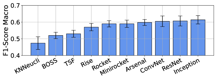
Figure 3. Average classifiers detection score through all the detection cases and all the datasets.

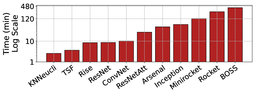
Figure 4. Average running time per run (training + inference time) for all classifiers (log scale y-axis).

5.1. Accuracy for 30min Sampling Frequency

The appliance detection results of the classifiers for the sampling frequency of 30min are summarized in Table 2. We observe that all classifiers return poor results for the UKDALE dataset. (We discuss and explain these results in detail in Section 5.3.) Furthermore, we note that independently of the dataset, some appliances are easier to detect than others. The following sections provide an analysis of these results according to the type of appliances.

5.1.1. Tech Appliances

Desktop Computer and Television seem to be well detected in the REFIT dataset, with a Macro F1-Score above 0.7 for the best classifiers. The score obtained on Desktop Computer on other datasets is not as good, but is consistent with the number of time series provided. It can be explained by the fact that the pattern is hidden behind other appliance activation signatures in longer smart meters load curves, and thus, is hard for classifiers to detect.

5.1.2. Kitchen Appliances

First, detecting Kettle usage looks pretty challenging, with poor results obtained by all classifiers and a Macro F1-Score $\simeq 0.45$. Given that a kettle operates for relatively short periods, it is understandable that its activation may not be captured using 30min sampled data. Microwave oven and classic Oven are not well detected in the EDF datasets. However, the detection score obtained on REFIT by the best two classifiers is above $0.7$, thanks to the larger amount of data available for this case in REFIT. Finally, the Cooker is well detected on the CER dataset.

5.1.3. Washer Appliances

Classifiers achieve promising results detecting Dishwasher and Tumble Dryer through CER and EDF 2 datasets. The lower performance obtained with the EDF 1 datast is explained by the lower amount of labeled instances given for these cases. However, the low score results obtained on the three washer appliances for REFIT are not due to the amount of time series data. We believe that this poor detection score can be explained by the fact that these three devices are used in combination and have similar activation patterns; therefore, the classifiers cannot easily distinguish among them.

5.1.4. Heating Appliances

The best detection scores are achieved for Water Heater on the EDF 1 and EDF 2 datasets. In France, water heaters refer mainly to devices that heat water from a hot tank, and usually operate during hours with high consumption power levels (Hohne et al., 2019). The classifiers can effectively discern this type of pattern, even using 30min sampled data. The lower performance on the CER dataset can be attributed to the use of two types of water heaters in Ireland: instantaneous and tank-pumped. Instantaneous water heaters only operate on demand, resulting in high spikes of short duration. Using the same label for these two devices, which have different activation signatures, significantly impacts the performance of the classifiers. The results on heater detection are satisfying for the EDF datasets, and we assume that the score difference between EDF 1 and EDF 2 is mainly due to the span of the time period used for training the model. By providing a full year of electricity consumption, the model can more easily detect the heater pattern, since it trains with data during the high consumption levels of the winter season. The poor performance on the CER dataset for heater detection can be attributed to the fact that the heater label indicates the presence of a convector electric heater, which is typically used as a supplementary heat source in winter, rather than being the primary heat source for the home.

5.1.5. Other Appliances

Electric Vehicles are well detected on the EDF 1 dataset considering the restricted number of labeled instances that we have available. The lengthy recharging times of electric vehicles and the high power required, combined with the fact that recharging often occurs mainly during low-consumption night-time hours, can explain the good performance we observe.

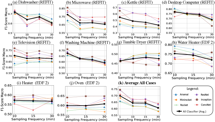
Figure 5. Influence of sampling frequency on different appliance detection cases. The detection score is given for each classifier and detection case following the resampling frequency of the data. The black line shows the average score of all the classifiers.

5.1.6. Overall Classifier Results Using 30min data

The overall results, shown in Table 2 and Figure 3, demonstrate that InceptionTime outperforms other classifiers when considering the average score and rank; InceptionTime is followed by ResNet, Arsenal, ConvNet, MiniRocket and Rocket. Since the ResNet model enhanced with the attention mechanism was not evaluated in all the cases, we do not include it in the total average score shown in Figure 3. However, this classifier achieves relatively poor performance compared to the others (refer to Table 2). In light of these results, it is essential to note the difference in performance between the best and worst performing classifiers: convolutional-based classifiers, i.e., InceptionTime, ConvNet and ResNet, are the optimal choice for many detection cases.

Figure 4 summarizes the average total running time (i.e., training and inference time together) for the 11 classifiers we studied. Taking into consideration the performance of the convolutional-based approaches (deep- and non deep-learning approaches), as well as their running time, we observe that this type of classifier is the most suitable for appliance detection using 30min sampled smart meter data. InceptionTime reaches a sligthly higher detection score, but at the cost of longer execution times. A balance between performance and efficiency is achieved by the ResNet and ConvNet classifiers.

5.2. Influence of Sampling Rate

In this part of the experimental evaluation, we analyze the improvement of the detection score of the different classifiers, as the smart meter sampling rate increases. We used the REFIT and EDF 2 datasets to perform these experiments, since these datasets provide data at a higher frequency than every 30min.

Using the REFIT dataset, we performed experiments at four different sampling rates: 1min, 10min, 15min, and 30min. To obtain complementary results on bigger appliances that were not available with REFIT data, we also included appliance detection cases from the EDF 2 dataset. However, since this dataset offers data sampled at 10 min, we could only produce results for sampling rates: 10min, 15min, and 30min.

All the results are summarized in Figure 5. For clarity, we only illustrate the scores of the five best classifiers.

On average across all cases, the appliance detection accuracy decreases significantly (by almost 0.1) when the sampling rate drops from 1min to 30min. For the best classifier (InceptionTime), the average drop is 0.15.

However, it is interesting to note that not all appliances are significantly better detected using a higher sampling frequency. As expected, appliances that operate only for short periods, i.e., Microwave or Kettle, benefit the most when using higher smart meter frequencies. For example, the results in Figure 5 show that using 1min sampled data can significantly improve the Kettle detection. In this case, the best classifier, ResNet, achieves a 0.2 improvement in the detection score when the sampling rate increases from 30min to 1min. For the Microwave case, it is a 0.1 average gain score for all the classifiers using 1min sampled data.

Other appliances, such as Dishwasher, Desktop Computer, Television, Washing Machine and Water Heater, which typically operate for long periods, are better detected using higher sampling rates, as well. For example, using 1min level data, the Washing Machine is much more accurately detected than when using 30min data (refer to Figure 5(f)).

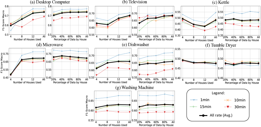
Figure 6. Results of the data imputation study using the REFIT dataset. For each appliance case, we can see on the left figure the evolution of the classification score according to the number of houses used, i.e., sources; on the right figure, we can see the evolution of the classification score according to the percentage of data used by houses.

5.3. Influence of Data Size

In this last part, we analyze the impact of the number of distinct households on classifier performance. These experiments demonstrate that classifiers cannot effectively learn the patterns of an appliance using only a small number of households when the smart meter data sampling frequency is very low (this explains the poor results presented in Section 5.1 for the UK-DALE dataset). Furthermore, we demonstrate that the number of households is more important for training the machine learning models than the amount of data available for each household.

We compared the following two approaches for training: (i) randomly select a subset of the houses and use all the data from these houses to train the models, and (ii) select all houses and use a random subset of the time series from each house. We performed the experiments on the appliance detection cases using the REFIT dataset. Furthermore, in order to account for the impact of the smart meter reading on these results, we performed the experiments using 4 different sampling frequencies: 1min, 10min, 15min, and 30min. Figure 6 summarizes the results of these experiments: the graphs show the average performance of all classifiers for each sampling rate. The black line represents the score value averaged across all sampling rates.

We note that for every sampling rate and detection case, it is almost always preferable to use all the available households and a subset of their time series, rather than to use all time series from a subset of the households. Indeed, data from the same house is frequently characterized by the consumption patterns of the residents. Instead, using data from multiple households, enables the classifier to focus on and learn the actual activation patterns of the appliances. Interestingly, using a subset of the households, or a subset of the time series does not seem to significantly affect the detection accuracy for the Washing Machine and the Tumble Dryer. The Tumble Dryer is indeed not well detected in our experiments. However, the detection score of the Washing Machine seems to be more impacted by the sampling frequency rather than by the data size.

6. Discussion

We now summarize the results of our evaluation. Figure 7 shows the average score for each classifier across all the experiments conducted in our study. The results show that the three deep learning-based methods are the most accurate overall. Among them, ResNet and ConvNet perform on average sligthly better than InceptionTime. However, as shown in Figure 8, the average score depends on the time series length. ResNet and ConvNet are better on average when using the short time series (REFIT and UKDALE datasets). InceptionTime is better on average when using long time series (CER and EDF datasets), because of InceptionTime’s ability to capture long-lasting patterns through the use of a combination of differently-sized kernels. Nevertheless, as the confidence intervals indicate, there is no clear winner among the three deep-learning classifiers. Based on these findings, we recommend using either ResNet or ConvNet, since their time performance is one order of magnitude faster than InceptionTime (see Figure 4).

Overall, the experiments show that for improving appliance detection, it is beneficial for electricity suppliers to collect data over extended periods of time, and at a finer time step than 30min. Indeed, a 15min step seems to be the minimum target in order to correctly detect a certain number of appliances. Furthermore, this study shows that further work is needed to more accurately detect appliances, even for data with 1min sampling frequency. Nevertheless, the lack of large electricity consumption public datasets that can be used to develop and train new algorithms is an important shortcoming. Having more good-quality data over long time intervals are necessary in order to allow for the development of more robust methods and further advancements in the field.

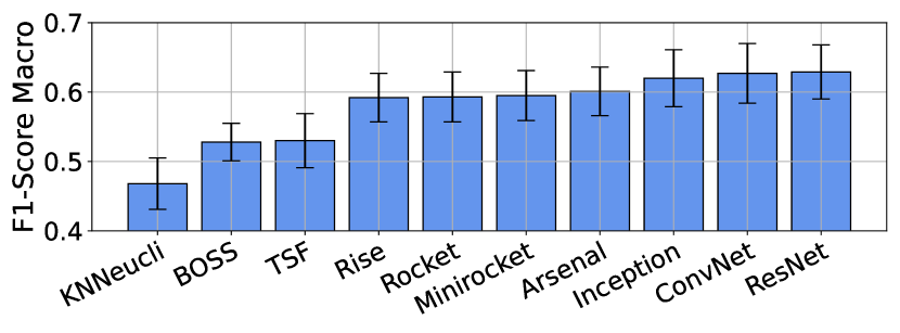
Figure 7. Average classifier detection score through all the experiments realized in this study (including sampling frequency influence and data size influence experiments).

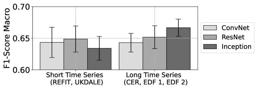
Figure 8. Average score of the 3 best classifiers (ConvNet, ResNet and InceptionTime) according to the time series length (i.e., datasets).

7. Conclusions

This paper presents a comprehensive evaluation of state-of-the-art time series classifiers applied to the appliance detection in very low-frequency smart meter data. We develop the first benchmark of time series classifiers for appliance detection using five different real datasets of very low-frequency electricity consumption with varying time series lengths. The results indicate that the performance of current time series classifiers varies significantly; only appliances that operate during long periods of time can be accurately detected using 30min sampled data. However, using 1min sampling data can drastically increase the detection accuracy of small appliances. Furthermore, deep learning-based classifiers have shown promising results in terms of accuracy, particularly for certain appliances. Overall, this study provides a valuable contribution to electricity suppliers, as well as analysts and practitioners, in order to help them choose the appropriate classifier for accurately detecting appliances in very low-frequency smart meter data.

References

- (1)
- CER (2012) 2012. CER Smart Metering Project - Electricity Customer Behaviour Trial, 2009-2010. https://www.ucd.ie/issda/data/commissionforenergyregulationcer/
- Albert and Rajagopal (2013) Adrian Albert and Ram Rajagopal. 2013. Smart Meter Driven Segmentation: What Your Consumption Says About You. IEEE Transactions on Power Systems 28, 4 (2013), 4019–4030. https://doi.org/10.1109/TPWRS.2013.2266122
- Allcott (2011) Hunt Allcott. 2011. Social norms and energy conservation. Journal of Public Economics 95, 9 (2011), 1082–1095. https://doi.org/10.1016/j.jpubeco.2011.03.003 Special Issue: The Role of Firms in Tax Systems.
- Aslan and Nur Zurel (2022) Muzaffer Aslan and Ebra Nur Zurel. 2022. An efficient hybrid model for appliances classification based on time series features. Energy and Buildings 266 (2022), 112087. https://doi.org/10.1016/j.enbuild.2022.112087
- Bagnall et al. (2016) Anthony Bagnall, Aaron Bostrom, James Large, and Jason Lines. 2016. The Great Time Series Classification Bake Off: An Experimental Evaluation of Recently Proposed Algorithms. Extended Version. https://doi.org/10.48550/ARXIV.1602.01711
- Barai et al. (2015) Gouri R. Barai, Sridhar Krishnan, and Bala Venkatesh. 2015. Smart metering and functionalities of smart meters in smart grid - a review. In 2015 IEEE Electrical Power and Energy Conference (EPEC). 138–145. https://doi.org/10.1109/EPEC.2015.7379940
- Boniol et al. (2022) Paul Boniol, Mohammed Meftah, Emmanuel Remy, and Themis Palpanas. 2022. DCAM: Dimension-Wise Class Activation Map for Explaining Multivariate Data Series Classification. In Proceedings of the 2022 International Conference on Management of Data (Philadelphia, PA, USA) (SIGMOD ’22). Association for Computing Machinery, New York, NY, USA, 1175–1189. https://doi.org/10.1145/3514221.3526183
- Breiman (2001) L Breiman. 2001. Random Forests. Machine Learning 45 (10 2001), 5–32. https://doi.org/10.1023/A:1010950718922
- Chavan et al. (2022) Deepika R. Chavan, Dagadu S. More, and Amruta M. Khot. 2022. IEDL: Indian Energy Dataset with Low frequency for NILM. Energy Reports 8 (2022), 701–709. https://doi.org/10.1016/j.egyr.2022.05.133 2022 The 4th International Conference on Clean Energy and Electrical Systems.
- Chren et al. (2016) Stanislav Chren, Bruno Rossi, and Tomáš Pitner. 2016. Smart grids deployments within EU projects: The role of smart meters. In 2016 Smart Cities Symposium Prague (SCSP). 1–5. https://doi.org/10.1109/SCSP.2016.7501033
- Cover and Hart (1967) T. Cover and P. Hart. 1967. Nearest neighbor pattern classification. IEEE Transactions on Information Theory 13, 1 (1967), 21–27. https://doi.org/10.1109/TIT.1967.1053964
- Dau et al. (2018) Hoang Anh Dau, Anthony Bagnall, Kaveh Kamgar, Chin-Chia Michael Yeh, Yan Zhu, Shaghayegh Gharghabi, Chotirat Ann Ratanamahatana, and Eamonn Keogh. 2018. The UCR Time Series Archive. https://doi.org/10.48550/ARXIV.1810.07758
- Dempster et al. (2019) Angus Dempster, François Petitjean, and Geoffrey I. Webb. 2019. ROCKET: Exceptionally fast and accurate time series classification using random convolutional kernels. CoRR abs/1910.13051 (2019). arXiv:1910.13051 http://arxiv.org/abs/1910.13051
- Dempster et al. (2021) Angus Dempster, Daniel F Schmidt, and Geoffrey I Webb. 2021. MiniRocket: A Very Fast (Almost) Deterministic Transform for Time Series Classification. In Proceedings of the 27th ACM SIGKDD Conference on Knowledge Discovery and Data Mining. ACM, New York, 248–257.
- Deng et al. (2022) Chunyu Deng, Kehe Wu, and Binbin Wang. 2022. Residential Appliance Detection Using Attention-based Deep Convolutional Neural Network. CSEE Journal of Power and Energy Systems 8, 2 (2022), 621–633. https://doi.org/10.17775/CSEEJPES.2020.03450
- Deng et al. (2013) Houtao Deng, George Runger, Eugene Tuv, and Martyanov Vladimir. 2013. A Time Series Forest for Classification and Feature Extraction. (2013). https://doi.org/10.48550/ARXIV.1302.2277
- Eibl and Engel (2015) Günther Eibl and Dominik Engel. 2015. Influence of Data Granularity on Smart Meter Privacy. IEEE Transactions on Smart Grid 6, 2 (2015), 930–939. https://doi.org/10.1109/TSG.2014.2376613
- Fawaz et al. (2020) Hassan Ismail Fawaz, Benjamin Lucas, Germain Forestier, Charlotte Pelletier, Daniel F. Schmidt, Jonathan Weber, Geoffrey I. Webb, Lhassane Idoumghar, Pierre-Alain Muller, and François Petitjean. 2020. InceptionTime: Finding AlexNet for time series classification. Data Mining and Knowledge Discovery 34, 6 (sep 2020), 1936–1962. https://doi.org/10.1007/s10618-020-00710-y
- Firth et al. (2017) Steven Firth, Tom Kane, Vanda Dimitriou, Tarek Hassan, Farid Fouchal, Michael Coleman, and Lynda Webb. 2017. REFIT Smart Home dataset. (6 2017). https://doi.org/10.17028/rd.lboro.2070091.v1
- Hart (1992) G.W. Hart. 1992. Nonintrusive appliance load monitoring. Proc. IEEE 80, 12 (1992), 1870–1891. https://doi.org/10.1109/5.192069
- He et al. (2015) Kaiming He, Xiangyu Zhang, Shaoqing Ren, and Jian Sun. 2015. Deep Residual Learning for Image Recognition. https://doi.org/10.48550/ARXIV.1512.03385
- Hills et al. (2014) J. Hills, J. Lines, E. Baranauskas, et al. 2014. Classification of time series by shapelet transformation. Data Min Knowl Disc 28 (2014), 851–881. https://doi.org/10.1007/s10618-013-0322-1
- Hohne et al. (2019) P.A. Hohne, K. Kusakana, and B.P. Numbi. 2019. A review of water heating technologies: An application to the South African context. Energy Reports 5 (2019), 1–19. https://doi.org/10.1016/j.egyr.2018.10.013
- Huber et al. (2021) Patrick Huber, Alberto Calatroni, Andreas Rumsch, and Andrew Paice. 2021. Review on Deep Neural Networks Applied to Low-Frequency NILM. Energies 14, 9 (2021). https://doi.org/10.3390/en14092390
- Ioffe and Szegedy (2015) Sergey Ioffe and Christian Szegedy. 2015. Batch Normalization: Accelerating Deep Network Training by Reducing Internal Covariate Shift. https://doi.org/10.48550/ARXIV.1502.03167
- Ismail Fawaz et al. (2019) Hassan Ismail Fawaz, Germain Forestier, Jonathan Weber, Lhassane Idoumghar, and Pierre-Alain Muller. 2019. Deep Learning for Time Series Classification: A Review. Data Min. Knowl. Discov. 33, 4 (jul 2019), 917–963. https://doi.org/10.1007/s10618-019-00619-1
- Kahl et al. (2022) Matthias Kahl, Daniel Jorde, and Hans-Arno Jacobsen. 2022. Representation Learning for Appliance Recognition: A Comparison to Classical Machine Learning. https://doi.org/10.48550/ARXIV.2209.03759
- Kahl et al. (2017) Matthias Kahl, Anwar Ul Haq, Thomas Kriechbaumer, and Hans-Arno Jacobsen. 2017. A Comprehensive Feature Study for Appliance Recognition on High Frequency Energy Data. In Proceedings of the Eighth International Conference on Future Energy Systems (Shatin, Hong Kong) (e-Energy ’17). Association for Computing Machinery, New York, NY, USA, 121–131. https://doi.org/10.1145/3077839.3077845
- Kaselimi et al. (2022) Maria Kaselimi, Eftychios Protopapadakis, Athanasios Voulodimos, Nikolaos Doulamis, and Anastasios Doulamis. 2022. Towards Trustworthy Energy Disaggregation: A Review of Challenges, Methods, and Perspectives for Non-Intrusive Load Monitoring. Sensors 22 (08 2022), 5872. https://doi.org/10.3390/s22155872
- Kelly and Knottenbelt (2015a) Jack Kelly and William Knottenbelt. 2015a. Neural NILM. In Proceedings of the 2nd ACM International Conference on Embedded Systems for Energy-Efficient Built Environments. ACM. https://doi.org/10.1145/2821650.2821672
- Kelly and Knottenbelt (2015b) Jack Kelly and William Knottenbelt. 2015b. The UK-DALE dataset, domestic appliance-level electricity demand and whole-house demand from five UK homes. Scientific Data 2 (03 2015). https://doi.org/10.1038/sdata.2015.7
- Kolter (2011) J. Zico Kolter. 2011. REDD : A Public Data Set for Energy Disaggregation Research.
- Laviron et al. (2021) Pauline Laviron, Xueqi Dai, Bérénice Huquet, and Themis Palpanas. 2021. Electricity Demand Activation Extraction: From Known to Unknown Signatures, Using Similarity Search. In e-Energy ’21: The Twelfth ACM International Conference on Future Energy Systems, Virtual Event, Torino, Italy, 28 June - 2 July, 2021, Herman de Meer and Michela Meo (Eds.). ACM, 148–159. https://doi.org/10.1145/3447555.3464865
- Lin et al. (2013) Min Lin, Qiang Chen, and Shuicheng Yan. 2013. Network In Network. https://doi.org/10.48550/ARXIV.1312.4400
- Lines et al. (2016) Jason Lines, Sarah Taylor, and Anthony Bagnall. 2016. HIVE-COTE: The Hierarchical Vote Collective of Transformation-Based Ensembles for Time Series Classification. In 2016 IEEE 16th International Conference on Data Mining (ICDM). 1041–1046. https://doi.org/10.1109/ICDM.2016.0133
- Liu et al. (2021) Yu Liu, Congxiao Liu, Yiwen Shen, Xin Zhao, Shan Gao, and Xueliang Huang. 2021. Non-intrusive energy estimation using random forest based multi-label classification and integer linear programming. Energy Reports 7 (2021), 283–291. https://doi.org/10.1016/j.egyr.2021.08.045 2021 The 4th International Conference on Electrical Engineering and Green Energy.
- Lubba et al. (2019) Carl H Lubba, Sarab S Sethi, Philip Knaute, Simon R Schultz, Ben D Fulcher, and Nick S Jones. 2019. catch22: CAnonical Time-series CHaracteristics. https://doi.org/10.48550/ARXIV.1901.10200
- Löning et al. (2019) Markus Löning, Anthony Bagnall, Sajaysurya Ganesh, Viktor Kazakov, Jason Lines, and Franz J. Király. 2019. sktime: A Unified Interface for Machine Learning with Time Series. https://doi.org/10.48550/ARXIV.1909.07872
- Middlehurst et al. (2020a) Matthew Middlehurst, James Large, and Anthony Bagnall. 2020a. The Canonical Interval Forest (CIF) Classifier for Time Series Classification. In 2020 IEEE International Conference on Big Data (Big Data). IEEE. https://doi.org/10.1109/bigdata50022.2020.9378424
- Middlehurst et al. (2020b) Matthew Middlehurst, James Large, and Anthony J. Bagnall. 2020b. The Canonical Interval Forest (CIF) Classifier for Time Series Classification. CoRR abs/2008.09172 (2020). arXiv:2008.09172 https://arxiv.org/abs/2008.09172
- Middlehurst et al. (2021) Matthew Middlehurst, James Large, Michael Flynn, Jason Lines, Aaron Bostrom, and Anthony J. Bagnall. 2021. HIVE-COTE 2.0: a new meta ensemble for time series classification. CoRR abs/2104.07551 (2021). arXiv:2104.07551 https://arxiv.org/abs/2104.07551
- Milam and Kumar Venayagamoorthy (2014) Megan Milam and G. Kumar Venayagamoorthy. 2014. Smart meter deployment: US initiatives. In ISGT 2014. 1–5. https://doi.org/10.1109/ISGT.2014.6816507
- Miyasawa et al. (2019) Ayumu Miyasawa, Yu Fujimoto, and Yasuhiro Hayashi. 2019. Energy disaggregation based on smart metering data via semi-binary nonnegative matrix factorization. Energy and Buildings 183 (15 Jan. 2019), 547–558. https://doi.org/10.1016/j.enbuild.2018.10.030 Funding Information: Part of this work was supported by the Japan Science and Technology Agency , CREST [ JPMJCR15K5 ]. We are deeply grateful to the staff members of Informetis Co., Ltd,. and wish to thank them for providing real data and discussing the evaluation index. Publisher Copyright: © 2018.
- O’Shea and Nash (2015) Keiron O’Shea and Ryan Nash. 2015. An Introduction to Convolutional Neural Networks. CoRR abs/1511.08458 (2015). arXiv:1511.08458 http://arxiv.org/abs/1511.08458
- Paradiso et al. (2013) Francesca Paradiso, Federica Paganelli, Antonio Luchetta, Dino Giuli, and Pino Castrogiovanni. 2013. ANN-based appliance recognition from low-frequency energy monitoring data. In 2013 IEEE 14th International Symposium on ”A World of Wireless, Mobile and Multimedia Networks” (WoWMoM). 1–6. https://doi.org/10.1109/WoWMoM.2013.6583496
- Paszke et al. (2019) Adam Paszke, Sam Gross, Francisco Massa, Adam Lerer, James Bradbury, Gregory Chanan, Trevor Killeen, Zeming Lin, Natalia Gimelshein, Luca Antiga, Alban Desmaison, Andreas Köpf, Edward Yang, Zach DeVito, Martin Raison, Alykhan Tejani, Sasank Chilamkurthy, Benoit Steiner, Lu Fang, Junjie Bai, and Soumith Chintala. 2019. PyTorch: An Imperative Style, High-Performance Deep Learning Library. https://doi.org/10.48550/ARXIV.1912.01703
- Qu et al. (2023) Leitao Qu, Yaguang Kong, Meng Li, Wei Dong, Fan Zhang, and Hongbo Zou. 2023. A residual convolutional neural network with multi-block for appliance recognition in non-intrusive load identification. Energy and Buildings 281 (2023), 112749. https://doi.org/10.1016/j.enbuild.2022.112749
- Rossier et al. (2017) Florian Rossier, Philippe Lang, and Jean Hennebert. 2017. Near Real-Time Appliance Recognition Using Low Frequency Monitoring and Active Learning Methods. Energy Procedia 122 (2017), 691–696. https://doi.org/10.1016/j.egypro.2017.07.371 CISBAT 2017 International ConferenceFuture Buildings & Districts – Energy Efficiency from Nano to Urban Scale.
- Sakoe and Chiba (1978) H. Sakoe and S. Chiba. 1978. Dynamic programming algorithm optimization for spoken word recognition. IEEE Transactions on Acoustics, Speech, and Signal Processing 26, 1 (1978), 43–49. https://doi.org/10.1109/TASSP.1978.1163055
- Schapire (2013) Robert E Schapire. 2013. Explaining adaboost. In Empirical inference. Springer, 37–52.
- Schäfer (2015) Patrick Schäfer. 2015. The BOSS is concerned with time series classification in the presence of noise. Data Mining and Knowledge Discovery 29 (11 2015). https://doi.org/10.1007/s10618-014-0377-7
- Schäfer and Högqvist (2012) Patrick Schäfer and Mikael Högqvist. 2012. SFA: A symbolic fourier approximation and index for similarity search in high dimensional datasets. ACM International Conference Proceeding Series, 516 – 527. https://doi.org/10.1145/2247596.2247656
- Shifaz et al. (2019) Ahmed Shifaz, Charlotte Pelletier, François Petitjean, and Geoffrey I. Webb. 2019. TS-CHIEF: A Scalable and Accurate Forest Algorithm for Time Series Classification. CoRR abs/1906.10329 (2019). arXiv:1906.10329 http://arxiv.org/abs/1906.10329
- Simonyan and Zisserman (2015) K Simonyan and A Zisserman. 2015. Very deep convolutional networks for large-scale image recognition. 3rd International Conference on Learning Representations (ICLR 2015), 1–14.
- Sykiotis et al. (2022) Stavros Sykiotis, Maria Kaselimi, Anastasios Doulamis, and Nikolaos Doulamis. 2022. ELECTRIcity: An Efficient Transformer for Non-Intrusive Load Monitoring. Sensors 22, 8 (2022). https://doi.org/10.3390/s22082926
- Szegedy et al. (2014) Christian Szegedy, Wei Liu, Yangqing Jia, Pierre Sermanet, Scott Reed, Dragomir Anguelov, Dumitru Erhan, Vincent Vanhoucke, and Andrew Rabinovich. 2014. Going Deeper with Convolutions. https://doi.org/10.48550/ARXIV.1409.4842
- Tabatabaei et al. (2017) Seyed Mostafa Tabatabaei, Scott Dick, and Wilsun Xu. 2017. Toward Non-Intrusive Load Monitoring via Multi-Label Classification. IEEE Transactions on Smart Grid 8, 1 (2017), 26–40. https://doi.org/10.1109/TSG.2016.2584581
- Wang et al. (2016) Zhiguang Wang, Weizhong Yan, and Tim Oates. 2016. Time Series Classification from Scratch with Deep Neural Networks: A Strong Baseline. https://doi.org/10.48550/ARXIV.1611.06455
- Yue et al. (2020) Zhenrui Yue, Camilo Requena Witzig, Daniel Jorde, and Hans-Arno Jacobsen. 2020. BERT4NILM: A Bidirectional Transformer Model for Non-Intrusive Load Monitoring. In Proceedings of the 5th International Workshop on Non-Intrusive Load Monitoring (Virtual Event, Japan) (NILM’20). Association for Computing Machinery, New York, NY, USA, 89–93. https://doi.org/10.1145/3427771.3429390
- Zhao et al. (2016) Bochao Zhao, Lina Stankovic, and Vladimir Stankovic. 2016. On a Training-Less Solution for Non-Intrusive Appliance Load Monitoring Using Graph Signal Processing. IEEE Access 4 (2016), 1784–1799. https://doi.org/10.1109/ACCESS.2016.2557460
- Zhao et al. (2020) Bochao Zhao, Minxiang Ye, Lina Stankovic, and Vladimir Stankovic. 2020. Non-intrusive load disaggregation solutions for very low-rate smart meter data. Applied Energy 268 (2020), 114949. https://doi.org/10.1016/j.apenergy.2020.114949