WIMP decay as a possible Warm Dark Matter model
Abstract
The Weakly Interacting Massive Particles (WIMPs) have long been the favoured Cold Dark Matter (CDM) candidate in the standard CDM model. However, owing to great improvement in the experimental sensitivity in the past decade, some parameter space of the Supersymmetric (SUSY)-based WIMP model is ruled out. In addition, a massive stable WIMP as the CDM particle is also at variance with other astrophysical observables at small scales. We consider a model that addresses both these issues. In the model, the WIMP decays into a massive particle and radiation. We study the background evolution and the first order perturbation theory (coupled Einstein-Boltzmann equations) for this model and show that the dynamics can be captured by a single parameter , which is the ratio of the lighter mass and the comoving momentum of the decay particle. We incorporate the relevant equations in the existing Boltzmann code CLASS to compute the matter power spectra and Cosmic Microwave Background (CMB) angular power spectra. The decaying WIMP model is akin to a non-thermal Warm Dark Matter (WDM) model and suppresses matter power at small scales, which could alleviate several issues that plague the CDM model at small scales. We compare the predictions of the model with CMB and galaxy clustering data. As the model deviates from the CDM model at small scales, the evolution of the collapse fraction of matter in the universe is compared with the high-redshift Sloan Digital Sky Survey (SDSS) HI data. Both these data sets yield , which can be translated into the bounds on other parameters. In particular, we obtain the following lower bounds on the thermally-averaged self-annihilation cross-section of WIMPs, , and the lighter mass: and . The lower limit on is comparable to constraints on the mass of thermally-produced WDM particle. The limit on the self-annihilation cross-section greatly expands the available parameter space as compared to the stable WIMP scenario.
1 Introduction
The standard cosmological model has proved to be very successful during the past two decades. Among other probes, the measurement of CMB temperature and polarization anisotropies, galaxy clustering as revealed by large galaxy surveys, and the detection of high-redshift supernova 1a have been key to this success [1, 2, 3, 4]. An important ingredient of the concordance CDM model is the cold dark matter. Its properties are indirectly inferred based on many observations covering a wide range of length scales, from sub-galactic to cosmological, and epochs of the universe (e.g. [5, 6, 2, 3, 7]).
While CMB and galaxy clustering observations show that the CDM is a good candidate of dark matter for scales , there exist long-standing astrophysical issue with the model at smaller scales. The CDM N-body simulations predict an order of magnitude larger number of satellite galaxy of the Milky way as compared to the observed number[8, 9]. The N-body simulations based on the CDM model predict a cuspy profile at the center of galaxies but the observed profile is flat [10]. Another issue to emerge from the comparison of CDM N-body simulations with observations is the “too big to fail” problem [11, 12]. All these issues provide motivation to consider alternatives, which reproduce the successes of the CDM model on cosmological scales but differ from the CDM model at small scales. The discovery of many high-redshift galaxies with unusually high stellar mass by JWST (e.g. [13, 14]) could be pointing at models other than the CDM model. However, it is equally likely that the observed behaviour is owing to much higher star formation efficiency at high redshifts (e.g. [13] and references therein). This issue is still being debated so we shall not attempt to study the possible implication of these results in this paper.
In the CDM model, one of the possible candidates for the CDM particle is the Weakly Interacting Massive Particle (WIMP). Such massive, stable, particles arise naturally in the supersymmetric extension of the standard model of particle physics. The theory predicts the CDM energy density infrerred from cosmological observables for self-annihilation cross-section and WIMP masses in the range 10–1000 GeV (WIMP miracle, e.g.[15]). This coincidence has spurred many direct [16, 17, 18], indirect[19, 20, 21] and collider [22, 23] searches of the WIMP. However, even after extensive laboratory and astronomical searches, the WIMP dark matter is yet to be detected. Direct lab searches, based on the scattering of dark matter particles with heavey nuclei, are sensitive to both spin-dependent and spin-independent interactions (e.g. [16, 18]). These experiments have achieved unprecedented precision in the recent years and have begun to rule out parameter-space favoured by supersymmetric extensions of the standard model (e.g. [24, 25, 26, 27]). In light of this fact, one needs to explore extensions to WIMPs-based models. In this paper, we consider such a model in which the WIMP decays and one of the decay products of WIMPs acts as cold dark matter at late times. From theoretical perspective, this scenario allows us to expand the permissible space of parameters. Additionally, we show that such a model leave observable signatures on CMB and galaxy clustering data and has a bearing on the small-scale issue with the CDM paradigm and therefore is potentially detectable by the current and future cosmological data.
In section 2, we discuss our model in detail. We derive the phase space distribution function of the decay products of WIMPs and show how different phases of this process impact the background evolution of the universe— from the production of WIMPs after freeze out in the very early universe to the evolution of the decay products of WIMPs. In section 3, we derive the first order perturbation theory for the decay products in Newtonian-conformal gauge and discuss the novel features of this scenario. We also outline the steps followed to incorporate our model in the existing code CLASS[28]. In section 4 our main results are presented. In section 4.1, we consider a number of data sets to test our model: Planck CMB data, SDSS (BOSS) data, and the evolution of neutral hydrogen mass density from damped Lyman- data. We use likelihood data of the two-point angular correlation functions of temperature, polarisation, and lensing potential fluctuations from Planck 2018 CMB data [2] and baryon acoustic oscillation (BAO) data of luminous red galaxy (LRG) distribution from BOSS [29]. We determine posterior probabilities on relevant parameters using Montepython [30, 31] MCMC codes. The CMB and BAO data allow us to compare our model with the data for scales . To test at smaller scales, we compute the evolution of collapsed fraction of matter in the universe and compare our theoretical prediction against the inferred collapsed fraction of neutral hydrogen obtained from the SDSS Lyman data [32, 33]. Section 5 is reserved for summarizing our main results and concluding remarks. Unless specified otherwise, we consider the spatially-flat cosmological model with Planck best-fit cosmological parameters ([2]).
2 Decaying WIMP
We propose a scenario in which non-relativistic WIMPs of mass decay into a lighter particle of mass and a massless particle: . For simplicity, we assume the decay to be instantaneous at . The decay is assumed to be triggered after the freeze-out. This allows us to treat the processes of the freeze-out and the decay separately. We discuss the potential impact of this assumption in section 5.
Assuming the WIMPs to be highly non-relativistic at the time of decay (or the ratio of their momentum to energy is negligible), the comoving momentum of the lighter particle (we refer to the lighter particle as warm dark matter (WDM) in the rest of the paper as our model is akin to non-thermally produced warm dark matter particles) and the decay radiation is given by: . The abundance of the WDM and the radiation particles is equal to the relic abundance of WIMPs. Thus, from relativistic kinematics, we can construct the following phase-space distribution function for the decay products—WDM and radiation—of WIMPs:
| (2.1) |
We note that the WDM particles are not in thermal equilibrium. WDM particles can be either relativistic or non-relativistic at the epoch of decay. For , the WDM particle is relativistic but it could be non-relativistic if . denotes the comoving number density of WDM particles, defined such that: . In this paper, we follow the momentum and energy coordinates used by Ma and Bertschinger [34]. In this case, is the comoving momentum of the unperturbed particle and therefore is a constant. For this choice of momenta, the energy of the particle can be expressed as: .
The velocity of the WDM determines its free streaming length scale: . The corresponding wavenumber is defined as: . Major contribution to this integral arises from times when the particle is highly relativistic. The comoving free streaming length reaches a maximum at the epoch when the particle becomes non-relativistic (see e.g. [35] and references therein). But as , free streaming length continues to be important even after this epoch. In this paper we consider many cases ranging from every early decay when the WDM particle is born highly relativistic to late-decay scenarios in which the particle is non-relativistic at the time of WIMP decay. The free streaming scale determines the impact of the decay product on the growth of density perturbations. To quantify this effect we define a parameter:
| (2.2) |
This parameter denotes the mass to momentum ratio of the WDM. It signifies the ’coldness’ of the WDM particle i.e. in the limit , and the particle is highly non-relativistic at all epochs. For , . In this case, the particle is highly relativistic at birth and could mimic radiation even at late times.
In the next subsection, We briefly summarize the criteria needed for a viable decaying WIMP model.
2.1 New parameters
The decay introduces two more parameters, and , in addition to the self-annihilation cross section and particle mass when the WIMP is stable. We list below the requirements on these parameters from cosmological observables and give possible implication of this model.
-
1.
We start evolving the abundance of WIMPs before the freeze-out and, assuming s-wave annihilation, determine the final abundance of WIMPs for a given velocity-weighted cross-section and . The freeze-out occurs at (e.g. Fig. 4 in [36]), , the freeze-out temperature, corresponds to for a GeV WIMP. The final WIMP energy density is nearly independent of and can be determined from the relation: (Equation 26 of [36]. This issue is discussed in more detail in Appendix B), where is the self-annihilation cross-section of WIMPs and is their relative velocity. The relic abundance ; is the critical density at the current epoch. We only consider models for which the decay occurs after the freeze-out: . In addition, we have the basic kinematic requirement for the decay: .
-
2.
For a stable WIMP, to match the observed CDM energy density. The current upper bound on the nucleon-WIMP cross-section from Xenon experiments is for a mass range [16, 17, 18]. These results have ruled out a fraction of parameter-space favoured by supersymmetric extensions of the standard model (e.g. [24, 25, 26, 27]). Our proposed model can accommodate a larger range of self-annihilation cross-sections: the current background energy density of CDM is if is nonrelativistic at the current epoch. This is smaller by a factor of as compared to the case of a stable WIMP. In other words, the corresponding increase in relic abundance that results from smaller cross-section can partly be compensated for by having a lower mass WDM particle produced through decay. This could accommodate both smaller self-annihilation cross sections and a wider – parameter space. This would also be compatible with current experimental bounds if , as this is the smallest WIMP mass that can be probed by XENON-based experiments [16, 17, 18].
- 3.
-
4.
The WIMP decay pumps additional radiation into the universe. The fraction of radiation energy contributed by the massless decay product is:
(2.4) Here and correspond to the background energy density of CMB and three standard model neutrinos, respectively. In addition, the WDM also contributes to the radiation density before it turns non-relativistic which we discuss in a later section. Current Planck and big-bang Nucleosynthesis (BBN) results put strong constraints the radiation content of the universe. Planck results determine the relativistic neutrino degrees of freedom: (e.g. see [2] for details of joint CMB and BBN ). This limits the additional radiation injection to be less than 3% of the contribution of photons and neutrinos.
-
5.
As we will see in later sections, the most stringent constraints on the decay WIMP model arise from the perturbation analysis of the WDM particle. We defined in the foregoing which determines the ’coldness’ of the WDM particles. In addition to the constraint arising from the additional radiation energy density released in the decay process, the WDM particles should be sufficiently ’cool’ to allow formation of structures at scales of interest. We consider the perturbation theory of this particle in the next section.
3 Perturbation theory of non-thermal WDM
As indicated in the previous section, the main impact of decaying WIMPs can be captured in the parameter , which denotes the coldness of the WDM particle. In this section, we discuss in detail the linear perturbation theory of the decay products of WIMPs—WDM and radiation. These particles are produced with a phase space distribution given by Eq. (2.1). We work in the Newtonian gauge and follow the notation of [37] for metric perturbations ( and ) and [34] for matter variables.
3.1 Before the decay:
After the freeze-out, WIMPs behave as cold dark matter with comoving relic abundance as determined by their self-annihilation cross-section . The background energy density and pressure are given by:
| (3.1) |
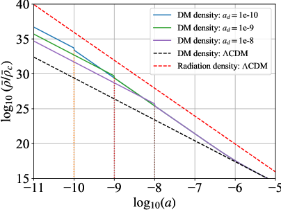
We note that the initial WIMP background density in our case is larger than the CDM model by a factor . This is because the decay products of WIMPs could behave as radiation for long periods after the decay (Figure 1) and, therefore, to satisfy the density constraint (Eq. (2.3)), the initial WIMP density has to be higher than for the case of a stable WIMP assumed in the CDM model.
In this case, the Boltzmann equations for density contrast and divergence component of the bulk velocity reduce to the usual CDM case (Equations (43) in [34]; for details of obtaining fluid equations from Boltzmann equations see e.g. [37]):
| (3.2) |
And the initial conditions for these variables are (Equations (97), (98) in [34]):
| (3.3) |
3.2 After the decay:
The WIMP decays into WDM and radiation. The WDM produced at decay is not necessarily either highly relativistic or non-relativistic. In most cases of interest to us in the paper, the WDM is born highly relativistic and make a transition to a non-relativistic particle during its evolution. In the general case, we cannot separate the and dependence in the WDM energy , and one has to numerically integrate over comoving momenta in the equations of Boltzmann hierarchy. However, unlike the usual case of HDM/WDM particles for which the phase space distribution of particles could be Fermi-Dirac distribution, the phase space distribution function in our cases is a delta function which allows us to analytically integrate over the momenta to obtain both the background density and pressure as well as the first order quantities: overdensity , bulk velocity , and shear stress .
To obtain background quantities, we plug in the WDM distribution function Eq. (2.1) into Equation (52) of [34], replace the relic abundance in favour of using (2.3) and . This yields:
| (3.4) |
Similarly, using Equation (55) in [34], one can calculate the 1st order quantities:
| (3.5) |
For the Boltzmann equations (Equation (57) in [34]), -dependence in the equations is integrated using the WDM distribution function over with , respectively. Using Eq. (3.5), we get:
| (3.6) |
Here can be defined in terms of the perturbed phase space distribution function (for details see [34]):
| (3.7) |
with
| (3.8) |
Here is the angle between the unit vectors of the Fourier mode and the particle momentum.
Finally, we use the following prescription to truncate the Boltzmann heirarchy (Equation (58) in [34]):
| (3.9) |
We take the initial conditions for WDM to match those of the WIMP at the time of decay. It should be noted that the entire set of perturbative equations depend only on two parameters: the mass-momentum ratio at the decay and the current DM density .
The dynamics of WDM perturbations also depend weakly on the epoch of decay through the background WIMP density Eq. ((3.1)) and the switch condition from CDM to WDM equations at . However, for the parameter space of interest to us, this dependence is negligible.
Next, we consider the equations corresponding to the radiation component of the decay. This component has the same phase space distribution function as the WDM (Eq. (2.1)). For radiation, the energy . We use Equation (44) of [34] to obtain the background quantities:
| (3.10) |
Similarly, Equation (47) of [34] yields the 1st order quantities:
| (3.11) |
And the -dependence in the Boltzmann equations (Equations (49) of [34]) can be integrated over since does not depend on . It should noted that even though the distribution function of this additional radiation component is different from that of massless neutrinos, the resulting equations are the same. More generally, so long as the and dependence of the energy can be separated i.e. in highly relativistic or completely non-relativistic case, the -dependence can be removed by integrating analytically. The relevant equations are:
| (3.12) |
We use the following condition to truncate the Boltzmann heirarchy (Equation (51) in [34]):
| (3.13) |
As for the WDM particle, the initial conditions for , and of this decay radiation are the same as that of WIMP at decay. This radiation component evolves as an independent species. Its contribution to the total radiation component of the universe is determined by and .
As anticipated in section 2.1, the dynamics of perturbations in our case is solely determined by the value of . The joining conditions at cause a very weak dependence of the results on the value of . One can verify that in the limit (non-relativistic limit), Eqs. (3.2) reduce to CDM equations (Eqs. (3.2)). In this case, the equations reduce to non-interacting fluid equations (continuity and Euler equations). All the higher order moments (Eqs. (3.9)) vanish as they are suppressed by powers of . On the other hand, for (relativistic limit), Eqs. (3.2) reduce to Eqs. (3.12), which give the evolution of perturbations of massless particles. It is also readily checked that the background quantities and matter variables (Eqs. (3.4) and (3.5)) also reduce to expressions appropriate for CDM and massless particles in these limits.
3.2.1 Matter-radiation equality
As the matter-radiation equality is determined with high precision by the Planck CMB data ( [2]), we briefly discuss how this epoch is altered in our case. Both the decay products of WIMPs contribute to radiation energy density in the universe. The WDM contributes to both the radiation and matter energy density: (Eq. (3.4)) and . Therefore, the total radiation density receives contribution from the decay radiation as well as the WDM in addition to photons and massless neutrinos, because of which the matter-radiation equality shifts closer to the current epoch as compared to the CDM case. At matter-radiation equality, ; is the background baryonic density. Using Eqs. (3.4) and (3.10), the scale factor can be determined from the condition:
| (3.14) |
3.3 CLASS implementation
Cosmic Linear Anisotropy Solving System [28] is one of the standard packages used for numerically solving coupled Einstein and Boltzmann equations for multiple coupled fluids in the context of cosmological perturbation theory. We modify the CLASS codes to add the relevant equations for the decay products—WDM and radiation—of the WIMP. The following major changes were made to the existing CDM model already implemented in CLASS:
-
1.
We added Eqs. (3.1)–(3.13) into relevant places in CLASS codes. The default parameter corresponding to the cold dark energy density is set to zero. Instead three new parameters , , and are used to quantify the WDM and the decay radiation ( is computed from (Eq. (3.10)). As noted above, is normalized to at . As shown in the foregoing, these parameters can be expressed in terms of parameters: , , , and .
- 2.
-
3.
For the perturbed components, Eqs. (3.2) are solved with initial conditions given by Eq. (3.3) for . At , we switch to Boltzmann equations for WDM (Eq. (3.2)) and radiation (Eq. (3.12)). The initial conditions at follow from the value of and of WIMPs at that time. Notice that as for WIMPs, both WDM and radiation inherit this initial condition. This situation is akin to the compensated mode when both massless neutrinos and primordial magnetic fields are present (e.g. [38]).
-
4.
An alternative way to incorporate WDM component in CLASS is through the non-cold dark matter option (using keyword ncdm). This allows one to input a distribution function different from the default Fermi-Dirac distribution used for massive neutrinos. We input the following distribution function to approximate the delta function:
We varied and studied its impact on the output. The procedure converges and yields the same results as obtained by direct inclusion of relevant equations in the code. We prefer the inclusion of relevant equations in CLASS over the ncdm option for the following reasons:
-
(a)
CLASS uses a number of approximation schemes—tight-coupling, ncdm fluid, free streaming, and ultra relativistic, to speed up the computation. For each of these approximations, CLASS computes the intervals within which they are valid. For the range of parameter space considered in our study, we find it difficult to match these conditions across the boundaries of their validity. Improper matching could result in sharp breaks and erroneous values at large scales in the matter power spectrum.
-
(b)
This approach still requires integration of the Boltzmann hierarchy over a grid of values. Thus, the computation cost is significantly increased as nearly 20 times (for 20 -bins) the number of equations have to be solved for each time step. The run time for such cases is about seconds. However, by solving the Boltzmann equations after integrating over brings the run time down to seconds.
-
(c)
The decay product corresponding to massless particles cannot be incorporated using only the ncdm option. As the fraction contributed by the additional radiation component is less than 0.3% of the total radiation for models of interest, its impact is negligible. It also allows us to compare the two methods.
More details of the implementation of our model in CLASS are given in the Appendix.
-
(a)
4 Results
In addition to CLASS implementation, we developed a Python code to numerically compute the matter power spectrum for a mutliple component fluid consisting of, in addition to WIMP and its decay products, photons, baryons, and massless neutrinos. For both our codes and CLASS runs we chose the following models/settings: (a) spatially flat universe with dark energy assumed to be cosmological constant, (b) adiabatic initial condition, (c) evolution from scale factor to . The other settings were chosen as the default settings for CLASS. The matter power spectra we obtain from our codes are in excellent agreement with CLASS results.
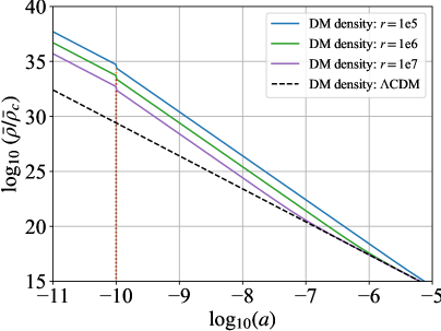
In Figure 1, we show the background evolution of the energy density of WDM for a range of decay times, and . All the models shown are normalized such that the energy density matches the observed CDM energy density at the current epoch.
The main difference between decaying WIMP and the CDM model emanates from two distinct reasons: (a) matter-radiation equality: From Eqs. (3.4) and (3.10), it is clear that both the decay products of WIMPs (WDM and radiation) contribute to radiation energy density. This can delay the matter radiation equality. For , we obtain , respectively. This leaves a detectable signature on both CMB and galaxy data. The joint analysis of Planck CMB and galaxy BAO data yields: [2]. (b) free-streaming of WDM: The free streaming of WDM hinders the formation of structures at sub-horizon scales. While this phenomenon effects a range of scales at different times, its impact can be approximately captured by the free-streaming length scale defined in the foregoing. We note that for .
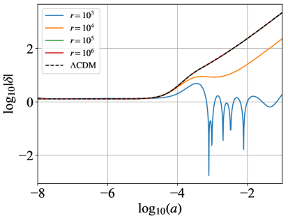
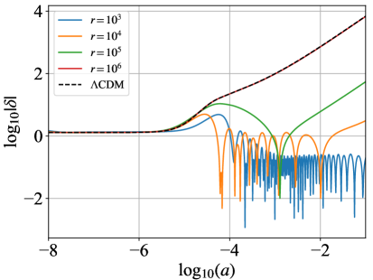
In Figure 2, we show the density evolution for two scales for different values of . The CDM model is also shown for comparison. The figure allows us to verify our understanding of the expected behaviour as changes. As noted above, the WDM is ’warmer’ for small . For , the perturbations oscillate and decay after horizon entry. This behaviour is akin to a massless neutrino. As is increased the particle becomes ’cooler’ and the power spectra approach the CDM model. The evolution of the mode is indistinguishable from the standard model for and . As both decaying WIMP and CDM models have identical evolution at super-horizon scales, the convergence towards the standard case is also more prominent for scales that enter the horizon later. For instance, the converges for larger value of as compared to the mode because this mode enters the horizon earlier. As the particle is hotter at earlier epochs, the density perturbations on smaller scales deviate more significantly from the CDM model.
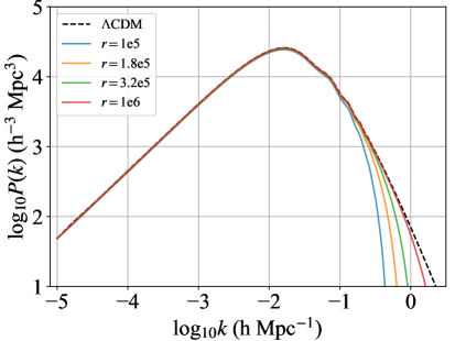
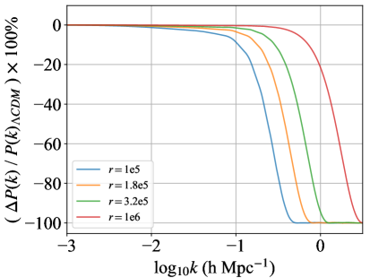
In Figure 3 we compare the linear matter power spectra for different . The results are in line with the evolution of density perturbations shown in Figure 2: the power on small scales is suppressed as these scale enter the horizon at earlier times when the particle is hotter. In the right panel we show the percentage difference between decaying WDM and CDM models, which show the scales at which the power is suppressed more clearly. The approximate scales of suppression can be gauged from the free-streaming scales: For , while it is nearly an order of magnitude larger for . These scales give the approximate point of departure between the CDM and WDM linear matter power spectra, for corresponding values of , in Figure 2.
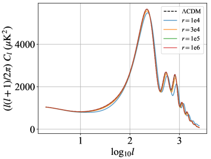
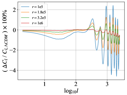
The impact of the altered dynamics on the CMB angular power spectrum is shown in Figure 4. The difference between our models and the CDM model arises owing to: (a) the suppression of matter power: this results in a reduction in the amplitude of CMB peaks, (b) increase in the expansion rate : additional radiation energy increases the expansion rate, which causes a decrease in the sound horizon () at the last scattering surface. As the angular scales of CMB peaks correspond to the multiples of the sound horizon, this causes the peaks to shift to smaller angular scales or larger . (a) and (b) together are responsible for the observed difference at shown in the right panel of Figure 4. In addition, an enhancement in the integrated Sachs-Wolfe effect owing to additional radiation component at the last scattering surface causes the angular power spectra to differ at smaller . As expected, the models approach the CDM model as increases.
Before undertaking detailed comparison of our models with data in the next section, we briefly discuss how cosmological observables might constrain parameters in our model. In our analysis, there are four parameters—, , , and —-and two constraints on and from cosmological observables (we do not list as a separate parameter, as it can be derived from these two parameters (Eq. (3.10))). For the models we consider the freeze out abundance of WIMPs, could be much larger than the abundance in the stable WIMP model (Figure 1), which requires to be smaller than to match the current mass density. The cosmological dark matter mass density and fixing the mass density to its best-fit value allows us to eliminate one parameter. The CMB anisotropies and galaxy clustering data puts a lower bound on (Eq. (2.2)). This constraint enables the elimination of another parameter which reduces the allowed parameter space from four to two. It follows from the two constraints that the allowed region is a region bounded by two surfaces—(i) (ii) , where are constants.
4.1 Data analysis
We compare our models based on linear perturbation theory against the available CMB and galaxy clustering data. In particular, we use Planck 2018 likelihood data of angular power spectra of temperature, polarisation (E mode) and lensing potential [2]. From SDSS data, we use the likelihood data of two-point correlation function of the distribution of Luminous Red Galaxies [29]. The CMB data estimates the angular power spectra for angular modes , which corresponds approximately to wavenumbers ( is the conformal time at the current epoch). The smallest scale that can be probed by low-redshift galaxy clustering data is also comparable as the density perturbations become non-linear at smaller scales.
The angular power spectra for temperature, polarisation (E mode) and lensing potential along with the matter power spectra are computed in CLASS codes for a given set of input parameters. The posteriors for these parameters are obtained using Montepython [31] implementation of MCMC. We choose Gaussian priors for the following seven parameters:
| Parameter | Mean | Std. Dev. | Lower lim | Upper lim |
|---|---|---|---|---|
| 100 | 2.2377 | 0.015 | _ | _ |
| 0.255 | 0.0026 | _ | _ | |
| 100 | 1.0411 | 0.0003 | _ | _ |
| 0.9659 | 0.0042 | _ | _ | |
| 3.0447 | 0.015 | _ | _ | |
| 0.0543 | 0.008 | 0.004 | _ | |
| 12.0 | 100.0 | 1.0 | 100.0 |
MCMC optimisation with combined likelihoods of Planck temperature, polarisation (E mode), Lensing angular power spectra along with the BAO data is performed with chains of steps each. As we have no prior information about the covariance of with the standard 6 parameters, we use the CDM covariance matrix with assumed to be independent for the first run. The ensuing chain is analysed to compute the covariance of with other parameters. The covariance matrix thus obtained is used for the subsequent runs. The average acceptance rate is and the radius of convergence . The best fit values and 1- and 2- errors on the estimated parameters are shown in Table 2
| Parameters | 2 > | 1 > | Best fit | Mean | 1 < | 2 < |
| 100 | 2.1989 | 2.2160 | 2.2233 | 2.2331 | 2.2505 | 2.2670 |
| 0.248 | 0.253 | 0.260 | 0.259 | 0.264 | 0.270 | |
| - | - | 89.726 | 54.148 | - | - | |
| 100 | 1.0419 | 1.0422 | 1.0424 | 1.0425 | 1.0427 | 1.0430 |
| ln | 3.0035 | 3.0188 | 3.0265 | 3.0338 | 3.0489 | 3.0649 |
| 0.9515 | 0.9567 | 0.9627 | 0.9623 | 0.9675 | 0.9731 | |
| 0.0388 | 0.0458 | 0.0512 | 0.0531 | 0.0602 | 0.0681 | |
| 65.426 | 66.241 | 66.828 | 67.079 | 67.913 | 68.753 | |
| 0.7999 | 0.8065 | 0.8099 | 0.8127 | 0.8189 | 0.8256 |
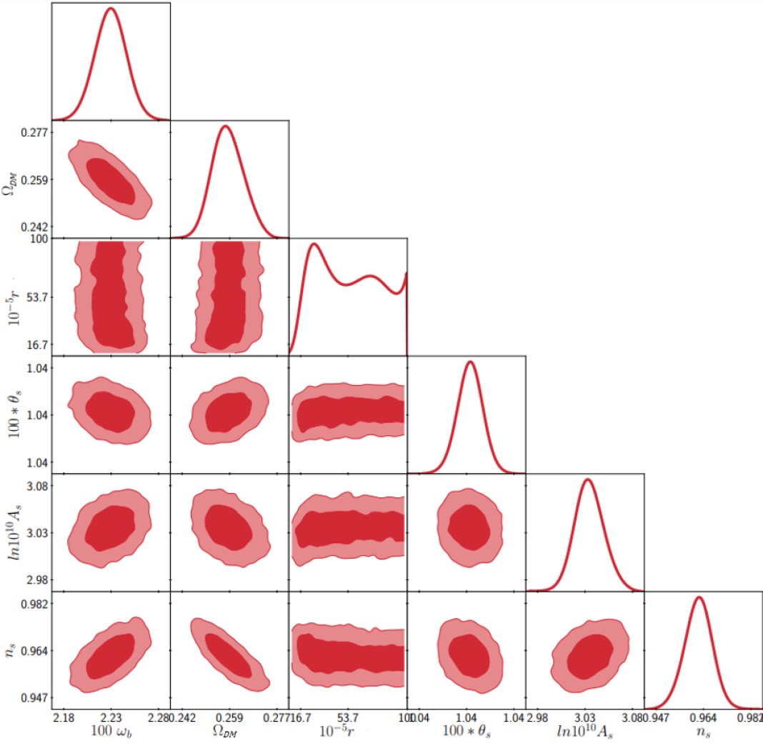
In Figure 5 we show the results of the MCMC analysis using the combined Planck 2018 CMB data along with the SDSS BAO data. The analysis yield an approximate lower bound: . The lower limit on implies the data is compatible with the CDM model. For , the corresponding free-streaming scale h Mpc-1 and the matter-radiation equality epoch, (Eq. (3.14)). From the contour plots between and other cosmological parameters, we note that the parameter is not constrained by the priors on other parameters.
4.1.1 Collapsed HI fraction
As noted above, the CMB and galaxy clustering data probe scales . The WDM models could deviate significantly from the CDM model at small scales. Some cosmological probes such as Weak gravitational lensing and Lyman- forest data allow probe of scales (e.g. [39, 7] and references therein). However, comparing our results with these data sets require extensive modelling which we consider beyond the scope of the current paper.
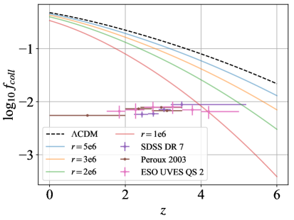
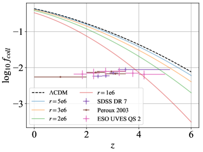
From absorption studies of high-redshift, QSOs, SDSS DR9 report the detection of nearly 7500 Damped Lyman- absorbers. This allows one to estimate precisely the average mass density of neutral hydrogen (HI) in the redshift range (see [32, 33] and reference therein; for more details see e.g. [40]). The mass density of HI can be related to the collapsed fraction of baryons and dark matter. This allows us to get an approximate measure of the minimum amount of collapsed fraction of the total matter in the redshift range . From the HI data one obtains, , which gives the fraction of the collapsed neutral hydrogen in terms of critical density of the universe . The (minimum) collapsed fraction is given by: , where is the background energy density of Baryons (for more details see section 5 of [41]).
For computing the collapsed fraction, , we integrate the Sheth-Tormen mass function [42] above a certain mass threshold. It is not straightforward to compare the theoretical collapsed fraction with the damped Lyman- data because there is a large uncertainty in the masses of these clouds. The simulations suggest that these clouds could be proto-galaxies with baryonic masses in the range (e.g. [43]). However, some recent observations suggest that the mass could be as high as at . ([44]). For the present work, we assume two halo masses and as the threshold masses for the formation of Damped Lyman- clouds. We compute the collapsed fraction for comparison with the data by integrating the mass function with threshold mass as lower limits.
In Figure 6 we display the collapsed fraction inferred from HI data against our models. The Figure shows that the evolution of collapsed fraction is an excellent diagnostic of small scale power, as the collapsed fraction for models with lower shows significant decrement at high redshifts. As the HI data gives a lower limit to the collapsed fraction, all the models that are well above the HI data could be deemed to acceptable. We can see that the collapsed fraction for WDM model corresponding to doesn’t meet this requirement at high redshifts. Therefore, this model can be ruled out. Much better bounds can be obtained with higher redshift data and greater information on the mass range of damped Lyman- clouds. The constraint on is of the same order as the one obtained from Planck CMB and BAO datasets.
5 Summary and Conclusion
In Figure 7 we show the constraints in – space for . The Figure displays the entire parameter space available in this case: and . The Figure also shows curves corresponding to a constant compatible with the Planck best-fit . We also display the allowed region arising from the total radiation fraction of decay products to be less than 1%. A lower bound on also constrains this fraction and we note that the data yields a stronger constraint. We summarize the main findings that follow from the figure. We also argue how the parameter space shown in Figure 7 can be generalized to other values of .
-
(a)
The minimum allowed WDM mass can be read off from Figure 7 for . This can be generalized to other WIMP masses. The lower limit on corresponds to . We define . It follows from the definition of (Eq. (2.2)):
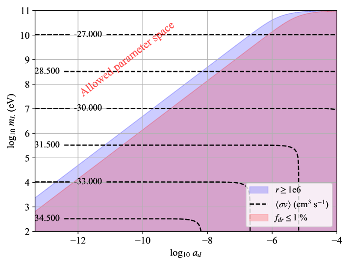
Figure 7: The figure shows the explored parameter space—, , and —and constraints from different cosmological observables for . The blue and the orange regions together are eliminated by the constraint and it follows from the analysis of CMB, galaxy clustering, and HI data (see text for detail). The orange region alone corresponds to the parameter space eliminated by the bound . This region is shown for comparison and underlines our result that the constraints obtained from the data are better than this bound. The black dashed lines display the Planck best-fit for a given . The lines are labelled by values of , e.g. -30 corresponds to . These lines are obtained by using Equation (26) of [36] and Eq. (2.3). (5.1) Notice that is dependent on the product of and . As Eq. (5.1) shows, the minimum mass arises from the earliest possible decay of WIMP. We assume the decay to be triggered after the freeze-out which implies a lower bound on . We assume (e.g. Fig. 4 in [36]). This prescription ensures that the decay process follows the freeze out epoch. This assumption yields an approximate lower bound keV. We note that similar lower bounds on the mass of thermally-produced WDM have been obtained from the comparison of these models with small-scale cosmological data (e.g. Lyman- and galactic data) at a range of scales (e.g. [45, 46, 47, 48]). The earliest possible decay of WIMP also yields the maximum relic abundance from Eq. (2.3) (or minimum self annihilation cross section which can be obtained by computing using Equation 26 of [36]), the minimum comoving energy of the decay radiation, and the maximum fraction of the decay radiation:
(5.2) We notice the maximum radiation fraction . In addition, the WDM contributes around 0.14% to the radiation density (see section 3.2.1 for detail). This is consistent with the bound on the fraction of radiation density displayed in Figure 7.
-
(b)
Figure 7 shows the range of allowed . The minimum decay redshift which arises from the requirement that for . The allowed range of follows from many related constraints: if is small and , WDM is highly relativistic at the time of decay. This scenario provides the minimum lower bound as the WDM is hotter if the decay occurs later. As is increased or the decay occurs at later times, the available parameter space shrinks as the lighter WDM particle are too hot and therefore prevent growth of structures. We note that the decay radiation could be photons if . In this case, the excess radiation gets thermalized with the plasma and doesn’t result in spectral distortion of the CMB spectrum (see e.g. [49, 50, 51, 40]). However, the decay into photons at can alter the light element abundance during primordial nucleosynthesis, which provides another constraint on such energy injection [52].
-
(c)
In Figure 7 we also show the contours of velocity-weighted cross-section that give the correct mass density for a given value of and . The intersection of these curves with the allowed region yields the set of parameters that satisfy all constraints. The allowed parameter space permits the range: ; Eq. (5.2) gives the minimum value of and its scaling with . Unlike the case of a stable WIMP which requires the self-annihilation cross section to lie in a narrow range nearly independent of the mass of WIMP (e.g. [36]), our proposed scenario expands the allowed parameter space by many orders of magnitude. We note that, given the range of self-annihilation cross-sections we explore in this paper, the particle interactions could be very different from a conventional WIMP. Even though such particles could fall within the WIMP family of models, it is conceivable such a particle arises from other physics.
In our analysis, we assumed the WIMP to have zero velocity at the time of decay which resulted in WDM phase-space distribution function to be a delta function. This is a good assumption as the decay particles are either highly relativistic at the time of decay or the decay occur late enough (the WIMP velocity decays as after the kinetic decoupling) to justify this assumption. In either case, the WIMP velocity is negligible as compared to the speeds of the decay products and therefore has negligible impact on our results. Our assumption also renders the problem analytically tractable and less expensive to implement numerically (CLASS runtime for the WDM model sec, which is comparable to the CDM model). One possible extension of our model would be to start with the more realistic Fermi distribution for the WIMPs.
In our analysis, we assume the decay of the particle to be instantaneous. In an expanding universe, instantaneous decay corresponds to the situation, . It is possible to consider extended decay or (e.g. by extending the formalism discussed by [53] for photons). In our analysis, we consider the processes of freeze-out and decay separately. A more comprehensive treatment would entail considering WIMPs as particles with a lifetime and solving the Boltzmann equations pertaining to their annihilation and decay simultaneously with the evolution of the background and the perturbed components of the multi-component fluid, which is be beyond the scope of this paper.
However, the results from the instantaneous decay model allow us to qualitatively discern the outcome of models with larger . In the instantaneous decay model, all the WDM particles produced have the same coldness parameter corresponding to and . If the lifetime pertains to a scale factor , the WDM particles will have a distribution of coldness parameters and the change in the power spectrum will be determined by a weighted mean of coldness parameters over the time of decay . The power suppression at any scale is determined by the velocity of the decay product at the time of horizon entry. The impact of finite decay time would be to spread the power suppression over a larger range of scales, which could lower the bound on .
Many alternative models to the WIMP-based CDM particle have been proposed, e.g. the WDM or ULA model (e.g. [54, 47] and references therein). However, even though our model is akin to non-thermal WDM scenario, it belongs in the WIMP-inspired family of models. In particular, it permits parameter space in the mass range which fell out of favour with improved sensitivity of XENON experiments [16, 18]. Our model also predicts the presence of a lighter particle whose presence can be revealed by the cosmological data. The current data puts a stringent lower bound on the mass of this particle, . Our proposed scenario could also alleviate some small-scale issues (e.g. cuspy profiles or missing satellites of the Milky way) of the stable WIMP model.
In addition, as the model uses parameter space of SUSY-based models, the heavier particle and/or its decay products might be detectable in collider experiments.
The past few decades have seen tremendous improvement in cosmological data and experimental sensitivity of XENON-based dark matter experiments. While cosmological data has thrown light on the nature of dark matter, its detection has eluded us. This has motivated theorists to move beyond the most-favoured model based on WIMPs. Our work suggests an alternative model that can be accommodated within the WIMP paradigm.
Acknowledgments
One of us (AP) sincerely thanks Dr. Harvinder Kaur Jassal for her invaluable advice and assistance during the research process. Additionally, we would like to extend our acknowledgement to Dr. Jasjeet Singh Bagla for his insights and suggestions regarding the halo mass function analysis.
Appendix A Appendix: CLASS implementation
The default configuration for both our own Python code and CLASS implementation (in explanatory.ini, the input parameter file): (i) Linear scalar perturbations in Newtonian gauge with adiabatic initial conditions (ii) Evolution from scale factor to (iii) Primordial helium fraction instead of default ’BBN’ for consistency of CLASS run with own Python code (iv) Power law primordial power spectrum with index for Gaussian fluctuations (v) 5 species: dark energy, dark matter, photons, baryons and massless neutrinos (vi) Spatially flat model () with the dark energy modelled as cosmological constant that only affects the background (vii) (viii) is set to , to with new variables and (ix) No massive neutrinos are considered and the only ultra relativistic species are the three massless neutrinos with . The other settings are the same as default settings for CLASS (which is configured for CDM model).
Here we list the CLASS files and the corresponding changes made in them to implement our model. We added two more species—warm dark matter and decay radiation—in the input, background and perturbations files.
input.c
-
•
In input_read_parameters_species(), we defined local variables flag4, flag5, param4, param5, has_wdm_userdefined in lines 2301-2313. The values for the parameters , , were read from the input in lines 2469-2508 with appropriate checks and stored in the structure background *pba. The value for was computed using (3.10) and stored.
-
•
The contribution of and to the total energy budget was added in lines 3207-3208.
-
•
Default values for , , , and were set to zero in lines 5738-5744.
background.h
-
•
The variables , , and were added to the structure background in lines 72-75.
-
•
Memory was allocated for index variables of the background density and pressure arrays for the dark matter and decay radiation in lines 174-177.
-
•
Conditional variable has_wdm was added in line 294. If its value is _TRUE_, it would mean both the WDM and decay radiation are present.
background.c
-
•
In background_functions(), local variables for density and pressure of WDM (, ) and decay radiation (, ) were added at lines 393-394.
-
•
, , and were computed using Eqs.(3.1), (3.4) and (3.10) in lines 447-460 based upon the condition . Prior to the decay, and were set to zero. The computed values were then stored in corresponding time arrays in structure background in lines 461-464. Their contribution to total density: , total pressure: , matter density: and radiation density: were added in lines 466-469.
- •
-
•
In background_indices(), default value of has_wdm is set to _FALSE_ in 1004 and is assigned _TRUE_ only if is non-zero in 1020-1021. The background density and pressure array indices are initialised in lines 1079-1083.
-
•
In background_solve(), non free-streaming dark matter fraction does not receive any contribution from WDM, see lines 2150-2162.
-
•
In background_initial_conditions(), the initial receives contribution from neither the dark matter, which is cold prior to the decay, nor the decay radiation (see lines 2254-2270).
-
•
In background_output_titles(), column titles ’rho_wdm’ and ’rho_decay_rad’ are added in lines 2502-2503.
-
•
In background_output_data(), the background time arrays for WDM and decay radiation are written, in lines 2579-2582.
-
•
In background_derivs(), WDM contributes to , see lines 2700-2702.
-
•
background_output_budget(), and are printed out, see lines 2873-2878.
perturbations.h
-
•
In structure perturbations, we added boolean variables for qualifying the presence of source and for WDM and decay radiation in lines 240, 241, 255, 256. Index variables for the same were added in lines 291, 292, 311, 312.
-
•
In structure perturbations_vector, time array indices for and maximum number of moments for WDM and decay radiation were added in lines 477-484.
perturbations.c
-
•
In background_output_data(), time array for over-density of WDM and decay radiation were written in lines 473-474 and 525-526.
-
•
Column titles of , and transfer function arrays of perturbations structure were stored in lines 565-566, 596-597 and 619-620.
-
•
Boolean variables for qualifying the presence of source and and index variables of perturbations structure were initialised in perturbations_indices().
-
•
WDM and decay radiation were added in the computation of maximum moment for any species in lines 2808-2809.
-
•
Column titles of arrays of perturbations_vector structure were stored in lines 3457-3462.
-
•
Time array indices for of perturbations_vector structure were initialised in 4055-4060.
-
•
Since we do not use any approximation schemes (tight coupling, ultra-relativistic, etc) for WDM or decay radiation, the values of , , are recopied into the original array perturbations_vector structure in lines 4517-4536.
-
•
In perturbations_initial_conditions(), we define local variables frac_wdm, and . Radiation and matter density contributions from WDM and decay radiation are added in lines 5493-5497. frac_wdm is initialised in line 5547, which is later used in the computation of —a conversion factor between synchronous and Newtonian initial conditions.
-
•
The initial conditions for perturbations of both WDM and decay radiation are taken from CDM initial conditions (Eq. (3.3)) in lines 5946-5957.
- •
-
•
In perturbations_total_stress_energy(), we add the WDM and decay radiation contributions to and in lines 7097-7103. The WDM contribution to and is added in lines 7105-7111.
-
•
In perturbations_print_variables(), local variables for , , are defined and initialised with the computed time arrays of perturbations_vector structure in lines 8451-8457, to be stored in lines 8678-8683, without any gauge transformation required since we use Boltzmann equations in Newtonian gauge. CLASS by default is implemented in synchronous gauge and transformed to the Newtonian gauge, if required by input. Our WDM implementation will work only for Newtonian gauge input.
-
•
In perturbations_derivs(), we define and initialise local variables and with their corresponding values in structure background. For WDM, we compute the derivatives of using Eq. (3.2) for and Eq. (3.2) otherwise. For decay radiation, we compute the derivatives of using Eq. (3.2) for and Eq. (3.12) otherwise.
Appendix B Appendix: Freeze-out
The fitting function given in Equation 26 of [36] was obtained for cross-sections in the range . In our work, we use cross-sections in the range . For smaller cross-sections the freeze-out occurs when the particle is still semi-relativistic. To address this issue we numerically solve the relevant Boltzman equation to obtain the relation between the relic abundance and the thermally-averaged cross-section. We obtain the following fit:
| (B.1) |
Eqs. (B.1) and (5.2) are in good agreement in the range . Using , the epoch of freeze-out for is and for , . Therefore, for lower , , we have semi-relativistic freeze-out, which does introduce some difference between and (B.1), which gives . However the difference is negligible. Eq. (5.2) provides a good fit to both Equation 26 of [36] and Eq. (B.1).
References
- [1] G. Hinshaw, D. Larson, E. Komatsu, D.N. Spergel, C. Bennett, J. Dunkley et al., Nine-year wilkinson microwave anisotropy probe (wmap) observations: cosmological parameter results, The Astrophysical Journal Supplement Series 208 (2013) 19.
- [2] N. Aghanim, Y. Akrami, M. Ashdown, J. Aumont, C. Baccigalupi, M. Ballardini et al., Planck 2018 results-vi. cosmological parameters, Astronomy & Astrophysics 641 (2020) A6.
- [3] B. Abolfathi, D. Aguado, G. Aguilar, C.A. Prieto, A. Almeida, T.T. Ananna et al., The fourteenth data release of the sloan digital sky survey: First spectroscopic data from the extended baryon oscillation spectroscopic survey and from the second phase of the apache point observatory galactic evolution experiment, The Astrophysical Journal Supplement Series 235 (2018) 42.
- [4] A. Conley, J. Guy, M. Sullivan, N. Regnault, P. Astier, C. Balland et al., Supernova constraints and systematic uncertainties from the first three years of the supernova legacy survey, The Astrophysical Journal Supplement Series 192 (2010) 1.
- [5] F. Zwicky, Republication of: The redshift of extragalactic nebulae, General Relativity and Gravitation 41 (2009) 207.
- [6] K.C. Freeman, On the Disks of Spiral and S0 Galaxies, The Astrophysical Journal 160 (1970) 811.
- [7] M. Bartelmann and P. Schneider, Weak gravitational lensing, Physics Reports 340 (2001) 291.
- [8] B. Moore, S. Ghigna, F. Governato, G. Lake, T. Quinn, J. Stadel et al., Dark matter substructure within galactic halos, The Astrophysical Journal Letters 524 (1999) L19.
- [9] A. Klypin, A.V. Kravtsov, O. Valenzuela and F. Prada, Where are the missing galactic satellites?, The Astrophysical Journal 522 (1999) 82.
- [10] G. Gentile, P. Salucci, U. Klein, D. Vergani and P. Kalberla, The cored distribution of dark matter in spiral galaxies, Monthly Notices of the Royal Astronomical Society 351 (2004) 903.
- [11] S. Garrison-Kimmel, M. Boylan-Kolchin, J.S. Bullock and E.N. Kirby, Too big to fail in the local group, Monthly Notices of the Royal Astronomical Society 444 (2014) 222.
- [12] M. Boylan-Kolchin, J.S. Bullock and M. Kaplinghat, Too big to fail? the puzzling darkness of massive milky way subhaloes, Monthly Notices of the Royal Astronomical Society: Letters 415 (2011) L40.
- [13] C.T. Donnan, D.J. McLeod, J.S. Dunlop, R.J. McLure, A.C. Carnall, R. Begley et al., The evolution of the galaxy UV luminosity function at redshifts z 8 - 15 from deep JWST and ground-based near-infrared imaging, Monthly Notices of the Royal Astronomical Society 518 (2023) 6011 [2207.12356].
- [14] I. Labbé, P. van Dokkum, E. Nelson, R. Bezanson, K.A. Suess, J. Leja et al., A population of red candidate massive galaxies 600 Myr after the Big Bang, Nature 616 (2023) 266 [2207.12446].
- [15] N. Craig and A. Katz, The fraternal wimp miracle, Journal of Cosmology and Astroparticle Physics 2015 (2015) 054.
- [16] XENON Collaboration 7 collaboration, Dark matter search results from a one ton-year exposure of xenon1t, Phys. Rev. Lett. 121 (2018) 111302.
- [17] Z. Ahmed, D. Akerib, S. Arrenberg, C. Bailey, D. Balakishiyeva, L. Baudis et al., Results from a low-energy analysis of the cdms ii germanium data, Physical Review Letters 106 (2011) 131302.
- [18] LUX Collaboration collaboration, Limits on spin-dependent wimp-nucleon cross section obtained from the complete lux exposure, Phys. Rev. Lett. 118 (2017) 251302.
- [19] O. Adriani, G. Barbarino, G. Bazilevskaya, R. Bellotti, M. Boezio, E. Bogomolov et al., Pamela results on the cosmic-ray antiproton flux from 60 mev to 180 gev in kinetic energy, Physical Review Letters 105 (2010) 121101.
- [20] M. Ackermann, M. Ajello, A. Allafort, W. Atwood, L. Baldini, G. Barbiellini et al., Measurement of separate cosmic-ray electron and positron spectra with the fermi large area telescope, Physical Review Letters 108 (2012) 011103.
- [21] M. Aguilar, J. Alcaraz, J. Allaby, B. Alpat, G. Ambrosi, H. Anderhub et al., Cosmic-ray positron fraction measurement from 1 to 30 gev with ams-01, Physics Letters B 646 (2007) 145.
- [22] J. Goodman, M. Ibe, A. Rajaraman, W. Shepherd, T.M. Tait and H.-B. Yu, Constraints on light majorana dark matter from colliders, Physics Letters B 695 (2011) 185.
- [23] P.J. Fox, R. Harnik, J. Kopp and Y. Tsai, Missing energy signatures of dark matter at the lhc, Physical Review D 85 (2012) 056011.
- [24] O. Buchmueller, R. Cavanaugh, A. De Roeck, M.J. Dolan, J.R. Ellis, H. Flächer et al., Higgs and supersymmetry, European Physical Journal C 72 (2012) 2020 [1112.3564].
- [25] L. Roszkowski, E.M. Sessolo and S. Trojanowski, WIMP dark matter candidates and searches—current status and future prospects, Reports on Progress in Physics 81 (2018) 066201 [1707.06277].
- [26] M. Schumann, Direct detection of WIMP dark matter: concepts and status, Journal of Physics G Nuclear Physics 46 (2019) 103003 [1903.03026].
- [27] C. Strege, G. Bertone, G.J. Besjes, S. Caron, R. Ruiz de Austri, A. Strubig et al., Profile likelihood maps of a 15-dimensional MSSM, Journal of High Energy Physics 2014 (2014) 81 [1405.0622].
- [28] D. Blas, J. Lesgourgues and T. Tram, The cosmic linear anisotropy solving system (CLASS). part II: Approximation schemes, Journal of Cosmology and Astroparticle Physics 2011 (2011) 034.
- [29] A. et al, The clustering of galaxies in the completed SDSS-III baryon oscillation spectroscopic survey: cosmological analysis of the DR12 galaxy sample, Monthly Notices of the Royal Astronomical Society 470 (2017) 2617.
- [30] B. Audren, J. Lesgourgues, K. Benabed and S. Prunet, Conservative Constraints on Early Cosmology: an illustration of the Monte Python cosmological parameter inference code, JCAP 1302 (2013) 001 [1210.7183].
- [31] T. Brinckmann and J. Lesgourgues, MontePython 3: boosted MCMC sampler and other features, 1804.07261.
- [32] P. Noterdaeme, P. Petitjean, C. Ledoux and R. Srianand, Evolution of the cosmological mass density of neutral gas from sloan digital sky survey II – data release 7, Astronomy & Astrophysics 505 (2009) 1087.
- [33] C. Pé roux, R.G. McMahon, L.J. Storrie-Lombardi and M.J. Irwin, The evolution of omega(hi) and the epoch of formation of damped lyman-alpha absorbers, Monthly Notices of the Royal Astronomical Society 346 (2003) 1103.
- [34] C.-P. Ma and E. Bertschinger, Cosmological perturbation theory in the synchronous and conformal newtonian gauges, The Astrophysical Journal 455 (1995) 7.
- [35] J. Lesgourgues and S. Pastor, Massive neutrinos and cosmology, Physics Reports 429 (2006) 307 [astro-ph/0603494].
- [36] G. Steigman, B. Dasgupta and J.F. Beacom, Precise relic WIMP abundance and its impact on searches for dark matter annihilation, Physical Review D 86 (2012) .
- [37] S. Dodelson, Modern Cosmology, Academic Press, Elsevier Science (2003).
- [38] J.R. Shaw and A. Lewis, Massive neutrinos and magnetic fields in the early universe, Physical Review D 81 (2010) 043517 [0911.2714].
- [39] M. McQuinn, The evolution of the intergalactic medium, Annual Review of Astronomy and Astrophysics 54 (2016) 313.
- [40] P.J.E. Peebles, Principles of Physical Cosmology, Princeton University Press (1993).
- [41] A. Sarkar, R. Mondal, S. Das, S. Sethi, S. Bharadwaj and D.J. Marsh, The effects of the small-scale DM power on the cosmological neutral hydrogen (HI) distribution at high redshifts, Journal of Cosmology and Astroparticle Physics 2016 (2016) 012.
- [42] R.K. Sheth and G. Tormen, Large-scale bias and the peak background split, Monthly Notices of the Royal Astronomical Society 308 (1999) 119 [astro-ph/9901122].
- [43] A. Pontzen, F. Governato, M. Pettini, C.M. Booth, G. Stinson, J. Wadsley et al., Damped Lyman systems in galaxy formation simulations, Monthly Notices of the Royal Astronomical Society 390 (2008) 1349 [0804.4474].
- [44] A. Font-Ribera, J. Miralda-Escudé, E. Arnau, B. Carithers, K.-G. Lee, P. Noterdaeme et al., The large-scale cross-correlation of Damped Lyman alpha systems with the Lyman alpha forest: first measurements from BOSS, Journal of Cosmology and Astroparticle Physics 2012 (2012) 059 [1209.4596].
- [45] N. Banik, J. Bovy, G. Bertone, D. Erkal and T. de Boer, Novel constraints on the particle nature of dark matter from stellar streams, Journal of Cosmology and Astroparticle Physics 2021 (2021) 043.
- [46] A. Dekker, S. Ando, C.A. Correa and K.C.Y. Ng, Warm dark matter constraints using milky-way satellite observations and subhalo evolution modeling, 2021. 10.48550/ARXIV.2111.13137.
- [47] M. Viel, G.D. Becker, J.S. Bolton and M.G. Haehnelt, Warm dark matter as a solution to the small scale crisis: New constraints from high redshift lyman- forest data, Physical Review D 88 (2013) 043502.
- [48] V.K. Narayanan, D.N. Spergel, R. Dave and C.-P. Ma, Lyman-alpha forest constraints on the mass of warm dark matter and the shape of the linear power spectrum, arXiv preprint astro-ph/0005095 (2000) .
- [49] H. Tashiro, CMB spectral distortions and energy release in the early universe, Progress of Theoretical and Experimental Physics 2014 (2014) 06B107.
- [50] J. Chluba, M. Abitbol, N. Aghanim, Y. Ali-Haimoud, M. Alvarez, K. Basu et al., New horizons in cosmology with spectral distortions of the cosmic microwave background, arXiv preprint arXiv:1909.01593 (2019) .
- [51] A. Kogut, M.H. Abitbol, J. Chluba, J. Delabrouille, D. Fixsen, J.C. Hill et al., Cmb spectral distortions: Status and prospects, 2019.
- [52] V. Poulin, J. Lesgourgues and P.D. Serpico, Cosmological constraints on exotic injection of electromagnetic energy, Journal of Cosmology and Astroparticle Physics 2017 (2017) 043 [1610.10051].
- [53] J. Bernstein and S. Dodelson, Aspects of the Zel’dovich-Sunyaev mechanism, Physical Review D 41 (1990) 354.
- [54] D.J. Marsh, Axion cosmology, Physics Reports 643 (2016) 1.