Rethinking Data Augmentation for Tabular Data in Deep Learning

Abstract

Tabular data is the most widely used data format in machine learning (ML). While tree-based methods outperform DL-based methods in supervised learning, recent literature reports that self-supervised learning with Transformer-based models outperforms tree-based methods. In the existing literature on self-supervised learning for tabular data, contrastive learning is the predominant method. In contrastive learning, data augmentation is important to generate different views. However, data augmentation for tabular data has been difficult due to the unique structure and high complexity of tabular data. In addition, three main components are proposed together in existing methods: model structure, self-supervised learning methods, and data augmentation. Therefore, previous works have compared the performance without comprehensively considering these components, and it is not clear how each component affects the actual performance.

In this study, we focus on data augmentation to address these issues. We propose a novel data augmentation method, Mask Token Replacement (MTR), which replaces the mask token with a portion of each tokenized column; MTR takes advantage of the properties of Transformer, which is becoming the predominant DL-based architecture for tabular data, to perform data augmentation for each column embedding. Through experiments with 13 diverse public datasets in both supervised and self-supervised learning scenarios, we show that MTR achieves competitive performance against existing data augmentation methods and improves model performance. In addition, we discuss specific scenarios in which MTR is most effective and identify the scope of its application. The code is available at https://github.com/somaonishi/MTR/.

1 Introduction

Deep learning is a powerful approach to solving a wide range of machine learning problems, such as image classification, natural language processing, and speech recognition. In recent years, deep learning has achieved impressive results in these areas. In many cases, it outperforms traditional machine learning approaches. For tabular data, however, tree-based approaches such as XGBoost (Chen and Guestrin, 2016) and LigthGBM (Ke et al., 2017) dominate.

Although tree-based methods have achieved significant results in many applications, it has recently been reported that deep learning models, especially Transformer-based models, sometimes outperform tree-based methods (Gorishniy et al., 2021; Somepalli et al., 2021; Wang and Sun, 2022; Chen et al., 2023). However, Grinsztajn et al. (2022) and Shwartz-Ziv and Armon (2022) argue that these reports are insufficiently validated and that tree-based methods are still dominant. Since there are no established benchmarks for tabular data, such as ImageNet for computer vision or GLUE for NLP, this tree-based vs. deep learning trend is expected to continue for some time.

One of the main advantages of deep learning is the attractive ability to build multi-modal pipelines for problems where only part of the input is tabular and the other parts include image, text, audio, or other DL-friendly data. Such pipelines can then be trained end-to-end by gradient optimization for all modalities. This is especially useful for complex real-world problems where data comes from multiple sources and has different formats and structures. On the other hand, tree-based methods are limited to handling tabular data and cannot easily incorporate other types of data. In other words, improving the performance and robustness of deep learning on tabular data remains an important task.

Data augmentation is a powerful approach to further improve the performance and robustness of deep learning. Data augmentation has been widely used in image and language deep learning. However, data augmentation for tabular data is not well established. Due to the unique structure and high complexity of tabular data, it is difficult to apply existing data augmentation methods widely used for images and other types of data.

In recent years, self-supervised learning has also attracted the attention of researchers in the field of tabular data. In this field, contrastive learning such as SimCLR (Chen et al., 2020) has become mainstream, and data augmentation is considered important to achieve good performance. Therefore, new data augmentation adapted to the unique structure of tabular data is still needed to improve the performance of contrastive learning on tabular data.

We summarize the contributions of our paper as follows:

• We summarize data augmentations on existing tabular data and evaluate their performance on 13 diverse public datasets.

• We introduce MTR, a novel data augmentation that takes advantage of Transformer’s properties to be highly competitive against existing data augmentations.

• We discuss scenarios in which MTR is more effective than other methods.

2 Related work

Data augmentation is a technique used to improve the generalization performance and robustness of machine learning models. In the image domain, common methods include rotation, flipping, and cropping. More complex methods include Random Erasing (Zhong et al., 2020), Cutmix (Yun et al., 2019), Mixup (Zhang et al., 2017), Manifold Mixup (Verma et al., 2018), and various other methods have been proposed (Shorten and Khoshgoftaar, 2019). In addition, for the NLP task, approaches such as masking, reordering, and deleting words have been proposed  (Feng et al., 2021).

Recently, data augmentation using generative models such as GAN-based (Goodfellow et al., 2014) and diffusion-based (Song et al., 2021) have been proposed in the image domain (Antoniou et al., 2018; Mariani et al., 2018; Rashid et al., 2019; Bird et al., 2022; Trabucco et al., 2023; Azizi et al., 2023; Akrout et al., 2023; Xiao et al., 2023). In the tabular data domain, SMOTE (Chawla et al., 2002) and GAN-based (Schultz et al., 2023; Engelmann and Lessmann, 2021) methods have been proposed. Theoretically, they can be extended to data augmentation. On the other hand, applying the generative model to data augmentation involves additional computational costs that cannot be ignored.

Data augmentation in images is mostly proposed in the context of supervised learning, but in the case of tabular data, it is mostly proposed as an adjunct to self-supervised learning methods. Existing works on tabular data include autoencoder based (Hinton and Salakhutdinov, 2006; Vincent et al., 2008), masked modeling based (Yoon et al., 2020; Majmundar et al., 2022; Onishi et al., 2023) and contrastive learning based (Bahri et al., 2022; Ucar et al., 2021; Wang and Sun, 2022; Darabi et al., 2021; Somepalli et al., 2021; Hajiramezanali et al., 2022) have been proposed, and the recent mainstream is contrastive learning based. VIME (Yoon et al., 2020) and SCARF (Bahri et al., 2022) proposed a data augmentation that randomly masks the input data and replaces the masked values by sampling from the same column. Using this data augmentation, VIME introduced the tasks of reconstructing the original features and estimating the mask vector from the masked features into pre-training; SCARF performed contrast learning using two views of the original data and the corrupted data. SubTab (Ucar et al., 2021) and Transtab (Wang and Sun, 2022) introduced data augmentation to divide the input tabular data into multiple subsets. They performed contrastive learning using the features of the divided subsets. Contrastive Mixup (Darabi et al., 2021) uses manifold mixup to create different views for contrastive learning. SAINT (Somepalli et al., 2021) uses cutmix and manifold mixup to create different views for contrastive learning. Stab (Hajiramezanali et al., 2022) creates different views by applying a sparse matrix to the weights and performs SimSiam-like (Chen and He, 2021) contrastive learning.

Chen et al. (2023) proposed a novel Transformer structure for tabular data, introducing two types of data augmentation: FeatMix in the input layer and HiddenMix in the hidden layer. In addition, Excelformer and FeatMix perform transformations that take into account the amount of mutual information.

Thus, while self-supervised learning has been the focus of much research on tabular data, there has been insufficient research on data augmentation techniques.

3 Method

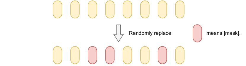
Figure 1: The demonstration of our method, MTR, a data augmentation method that randomly replaces part of the sequence of embedding tokenized by Tokenizer with [mask](red token).

In this section, we introduce our proposed method. Our data augmentation methods can be easily implemented by extending the existing Transformer model. First, given $k$ feature data $x\in\mathcal{X}\subseteq\mathbb{R}^{k}$, the Transformer model for tabular data transforms it into a sequence of embedding $T\in\mathbb{R}^{k\times d}$ using Tokenizer, where $d$ is the dimension of the embedding. Then, using a Transformer such as vanilla-Transformer (Vaswani et al., 2017), [cls]token, and Head which predicts the target from encoded [cls], the prediction is output from the sequence of embedding obtained as follows:

$$T=\mathtt{Tokenizer}(x) \in\mathbb{R}^{k\times d},$$

$$T^{\prime}=\mathtt{Append}[T,\mathtt{[cls]}] \in\mathbb{R}^{(k+1)\times d},$$

$$T_{\mathrm{encode}}=\mathtt{Transformer}(T^{\prime}) \in\mathbb{R}^{(k+1)\times d},$$

$$\hat{y}=\mathtt{Head}(T_{\mathrm{encode}}^{\mathtt{[cls]}}).$$

Our method focuses on a sequence of embedding $T$ generated by Tokenizer. Our method is simple: replace part of the sequence of embedding $T$ generated by Tokenizer with mask token ([mask]) (Devlin et al., 2019). See Figure 1. We call our method Mask Token Replacement (MTR). Based on the Bernoulli distribution of the probability $p_{m}$, MTR decides whether to replace the column embedding with [mask]or not (1: replace, 0: keep). Each [mask]is a learnable parameter that is shared among the columns.

4 Experiments

In this section, we perform two validations to demonstrate the effectiveness of our method.

• Experiment 1. Fully supervised with all train.

• Experiment 2. Self-supervised learning with 25% of train.

Datasets.

We use 13 diverse public datasets. For each dataset, we perform a split with $\mathtt{train}:\mathtt{val}:\mathtt{test}=6:2:2$. The same split is performed for all methods, and a different split is performed for each seed. val is truncated to 20,000 samples for speed. The datasets include: Jasmine (Guyon et al., 2019) (JA), Spambase (Dua and Graff, 2017) (SP), Philippine (Guyon et al., 2019) (PH), Wine Quality (Cortez et al., 2009) (WQ), Gesture Phase Segmentation (Dua and Graff, 2017) (GPS), Shrutime (SH), Online Shoppers(Sakar et al., 2019) (OS), FIFA (FI), California Housing (Pace and Barry, 1997) (CA), Bank Marketing (Moro et al., 2014) (BM), Adult  (Kohavi, 1996) (AD), Volkert (Guyon et al., 2019) (VO), Creditcard (Pozzolo et al., 2015) (CC). For the Wine Quality dataset, we follow the pointwise approach to learning-to-rank and treat ranking problems as regression problems. The dataset properties are summarized in Table 1.

Table 1: Dataset properties. Notation: “RMSE” ~ root-mean-square error, “ACC” ~ accuracy, “AUC” ~ area under the ROC curve.

Dataset	openml id	objects	features	metric	classes
JA	41143	2984	145	AUC	1
SP	44	4601	58	AUC	1
PH	41145	5832	309	AUC	1
WQ	287	6497	12	RMSE	-
GPS	4538	9873	33	ACC	5
SH	45062	10000	11	AUC	1
OS	45060	12330	18	AUC	1
FI	45012	19178	29	RMSE	-
CA	-	20640	9	RMSE	-
BM	1461	45211	17	AUC	1
AD	-	48842	15	AUC	1
VO	41166	58310	181	ACC	10
CC	1597	284807	30	AUC	1

Data preproccessing.

The same preprocessing is applied to all datasets. We apply quantile transformation to numerical features and ordinal encoder from Scikit-learn library (Pedregosa et al., 2011) to categorical features. We apply standardization to regression targets for all methods.

Model architecture.

In this paper, we perform all experiments using FTTransformer (Gorishniy et al., 2021) as the base model for all methods. The hyperparameters of the model follow the default hyperparameters proposed by Gorishniy et al. (2021). See our code for details.

Baseline.

We include the following baselines for comparison:

• w/o data augmentation (w/o DA). Used to compare model performance without data augmentation.

• Manifold Mixup (Verma et al., 2018). Apply in the latent space. The manifold mixup is applied to two $T_{\mathrm{encode},i}^{\mathtt{[cls]}},T_{\mathrm{encode},j}^{\mathtt{[cls]}}$ in the same batch encoded by Transformer with $\lambda=\mathrm{Beta}(\alpha,\alpha)$. Label-mixing is performed as $y_{i}=(1-\lambda)y_{i}+\lambda y_{j}$. The hyperparameter is $\alpha$. See our code for more details.

• Cutmix. Applied in the input space. It is applied to two inputs $x_{i},x_{j}\in\mathbb{R}^{k}$ in the same batch. Randomly select $\lfloor\lambda\times k\rfloor$ indices and swap the values of $x_{i},x_{j}$ corresponding to the selected indices. Note that $\lambda\sim\mathrm{Beta}(\alpha,\alpha)$. Also, according to the actual swapped rate $\lambda^{\prime}$, label-mixing is performed as $y_{i}=(1-\lambda^{\prime})y_{i}+\lambda^{\prime}y_{j}$. The hyperparameter is $\alpha$. See our code for more details.

• SCARF (Bahri et al., 2022). Applied in the input space. The mask vector $m$ generated from the Bernoulli distribution based on the mask fraction $p_{m}$ is used to determine the corruption points. When $m_{j}$ is 1, $x_{j}$ is replaced by $\hat{x}_{j}\sim\widehat{\mathcal{X}_{j}}$. Here $\widehat{\mathcal{X}_{j}}$ is assumed to be uniformly distributed over $\mathcal{X}_{j}=\{x_{j}:x\in\mathcal{X}\}$, where $\mathcal{X}$ is the training data. The hyperparameter is $p$. See our code for more details.

• HiddenMix (Chen et al., 2023). Applied in the latent space. For two $T_{i},T_{j}\in\mathbb{R}^{k\times d}$ in the same batch generated by Tokenizer, $T_{i}=S\odot T_{i}+(\mathbbm{1}-S)\odot T_{j}$. The coefficient matrix $S$ and the all-one matrix $\mathbbm{1}$ are of size $k\times d$. $S=[s_{1},s_{2},\ldots,s_{k}]^{\top}$, all whose vector $s_{h}\in\mathbb{R}^{d}$ ($h=1,2,\ldots,k$) are identical and have $\lfloor\lambda\times d\rfloor$ randomly selected elements of 1’s and the rest elements are 0’s. Note that $\lambda\sim\mathrm{Beta}(\alpha,\alpha)$. label-mixing is performed as $y_{i}=\lambda y_{i}+(1-\lambda)y_{j}$. The hyperparameter is $\alpha$. See our code for more details.

Supervised and self-supervised learning.

In supervised learning, we applied data augmentation with a probability of 50% for all methods and no data augmentation at test time. In self-supervised learning, we perform pre-training with contrastive learning. For the output $T_{\mathrm{encode}}^{\mathtt{[cls]}}$ of Transformer, we perform the transformation $z=\mathtt{PredictionHead}(T_{\mathrm{encode}}^{\mathtt{[cls]}})\in\mathbb{R}^{h}$, where $h$ is the dimension of the latent space. We applied this transformation to $\hat{T}_{\mathrm{encode}}^{\mathtt{[cls]}}$ with data augmentation and $T_{\mathrm{encode}}^{\mathtt{[cls]}}$ without data augmentation to obtain the vectors $\hat{z},z$. Then, we applied NT-Xent loss (Chen et al., 2020) to these two different views $\hat{z},z$ for contrast learning. Note that Cutmix was not included in the baseline in the self-supervised learning because it does not use the label-mixing, and therefore behaves almost the same as SCARF.

Training.

Table 2: Correspondence table betweentrain size and batch size.

train size	batch size
more than 50,000	1024
between 10,000 and 50,000	512
between 5,000 and 10,000	256
between 1,000 and 5,000	128
less than 1,000	64

We changed the batch size for all methods according to the size of the train (see Table 2). For supervised learning, we set the maximum training epochs to 500 for all methods. We also applied early stopping with patience of 15 using validation loss. For self-supervised learning, the early stopping patience was set to 10 and the maximum number of epochs was set to 200. The hyperparameters $\alpha$ of Manifold Mixup, Cutmix, and HiddenMix were set to $\alpha=\{0.1,0.2,0.5,0.75,1.0,1.5,2.0\}$, and the hyperparameters $p_{m}$ of SCARF and MTR was set to $p_{m}=\{0.1,0.2,0.5,2.00.1,0.2,0.3,0.4,0.5,0.6,0.7\}$.

In all of our experiments, we used the following two pieces of hardware; hardware 1 has an Intel(R) Xeon(R) Gold 6244 CPU with NVIDIA Quadro RTX 5000 GPU, and hardware 2 has an Intel(R) Xeon(R) Gold 6250 CPU with NVIDIA RTX A2000 12GB GPU.

4.1 Experiment 1. Supervised learning

Table 3: Results for the supervised learning. The metrics are averaged over 10 random seeds. For each dataset, the top result is in bold and the second result is in underline. For each dataset, ranks are computed by sorting the reported scores; the “Rank” column reports the average rank across all datasets.

Dataset JA ↑ SP ↑ PH ↑ WQ ↓ GPS ↑ w/o DA $85.06$ $98.53$ $80.78$ $0.6907$ $56.45$ Manifold Mixup ($\alpha$) $85.29$ (2.0) $98.48$ (0.1) $81.36$ (0.2) $\underline{0.6805}$ (0.75) $56.62$ (1.0) Cutmix ($\alpha$) $\underline{85.62}$ (1.5) $98.37$ (0.2) $81.53$ (1.0) $0.6814$ (0.2) $\underline{59.80}$ (1.0) SCARF ($p_{m}$) $85.30$ (0.4) $98.62$ (0.2) $81.41$ (0.7) $0.6819$ (0.2) $58.34$ (0.1) HiddenMix ($\alpha$) $85.38$ (2.0) $\mathbf{98.65}$ (0.5) $\underline{81.54}$ (1.0) $0.6809$ (1.5) $\mathbf{59.99}$ (0.75) MTR ($p_{m}$) $\mathbf{85.63}$ (0.6) $\underline{98.63}$ (0.7) $\mathbf{82.91}$ (0.7) $\mathbf{0.6804}$ (0.3) $57.55$ (0.2)

Dataset SH ↑ OS ↑ FI ↓ CA ↓ BM ↑ w/o DA $86.18$ $92.44$ $10100.0$ $0.4781$ $93.63$ Manifold Mixup ($\alpha$) $86.36$ (1.0) $\underline{92.55}$ (0.75) $9944.3$ (0.1) $0.4773$ (1.5) $93.64$ (2.0) Cutmix ($\alpha$) $\underline{86.46}$ (1.0) $92.37$ (0.2) $9814.5$ (0.5) $\underline{0.4691}$ (0.5) $93.64$ (0.1) SCARF ($p_{m}$) $\mathbf{86.46}$ (0.2) $92.43$ (0.1) $\mathbf{9690.1}$ (0.4) $0.4710$ (0.1) $93.67$ (0.1) HiddenMix ($\alpha$) $86.25$ (0.75) $\mathbf{92.62}$ (0.75) $9937.3$ (1.0) $0.4802$ (0.1) $\underline{93.72}$ (2.0) MTR ($p_{m}$) $86.33$ (0.5) $92.37$ (0.1) $\underline{9779.8}$ (0.6) $\mathbf{0.4675}$ (0.4) $\mathbf{93.78}$ (0.6)

Dataset AD ↑ VO ↑ CC ↑ Rank w/o DA $91.73$ $71.82$ $97.83$ $5.54$ Manifold Mixup ($\alpha$) $91.75$ (0.2) $71.92$ (0.5) $98.26$ (1.0) $4.08$ Cutmix ($\alpha$) $\underline{91.80}$ (2.0) $\mathbf{72.79}$ (0.5) $98.21$ (1.0) $3.08$ SCARF ($p_{m}$) $91.78$ (0.3) $\underline{72.43}$ (0.3) $\mathbf{98.38}$ (0.3) $\underline{2.85}$ HiddenMix ($\alpha$) $91.75$ (0.1) $72.27$ (0.75) $\underline{98.27}$ (2.0) $2.92$ MTR ($p_{m}$) $\mathbf{91.81}$ (0.5) $72.06$ (0.1) $98.20$ (0.4) $\mathbf{2.54}$

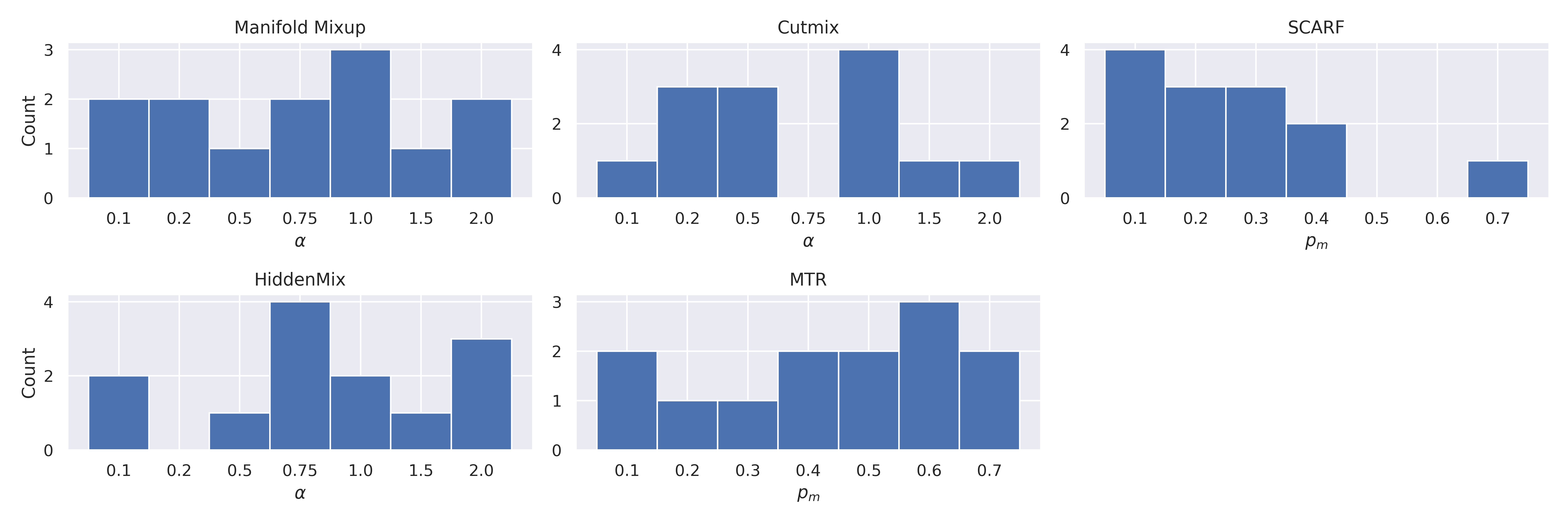
Figure 2: Comparison of hyperparameter distributions for different data augmentation methods in supervised learning. The histograms show the aggregated values of the hyperparameters for each of the data augmentation methods for all datasets.

Table 3 shows the results of supervised learning and Figure 2 shows the distribution of the selected best hyperparameters. Overall, the data augmentation methods improve the performance compared to the case without data augmentation (w/o DA). The proposed method, MTR, achieved competitive performance compared to other data augmentation methods. It achieved the highest average rank of 2.54, indicating that it is effective in improving model performance. In particular, it outperformed the other methods on PH dataset which has a large number of features.

SCARF, HiddenMix, and Cutmix were highly competitive with our methods. For SCARF, Bahri et al. (2022) claimed that a default $p_{m}$ between 0.5 and 0.7 is better, but we found that a lower $p_{m}$ is better in many cases in this experiment. HiddenMix and Cutmix significantly outperformed the proposed method on GPS and VO datasets for multi-class classification. This is because the label-mixing increases the diversity of the data. In fact, we confirmed that the accuracy of HiddenMix without label-mixing on GPS dataset was significantly lower – 57.99% (w/o label-mixing).

For Manifold Mixup, the overall performance was similar to that of w/o DA. The average rank was also lower than for other data augmentation methods.

4.2 Experiment 2. Self-supervised learning

Table 4: Results for the self-supervised learning. The metrics are averaged over 10 random seeds. For each dataset, the top result is in bold and the second result is in underline. For each dataset, ranks are computed by sorting the reported scores; the “Rank” column reports the average rank across all datasets.

Dataset JA ↑ SP ↑ PH ↑ WQ ↓ GPS ↑ Supervised $83.64$ $\mathbf{97.81}$ $76.70$ $0.7178$ $49.31$ Manifold Mixup ($\alpha$) $83.72$ (2.0) $97.71$ (2.0) $76.53$ (0.75) $0.7174$ (1.5) $49.41$ (2.0) SCARF ($p_{m}$) $\mathbf{84.20}$ (0.6) $97.61$ (0.6) $\underline{79.29}$ (0.7) $0.7153$ (0.1) $49.37$ (0.3) HiddenMix ($\alpha$) $83.78$ (1.0) $\underline{97.74}$ (1.5) $76.85$ (2.0) $\mathbf{0.7138}$ (0.75) $\mathbf{49.81}$ (0.5) MTR ($p_{m}$) $\underline{83.83}$ (0.5) $97.45$ (0.5) $\mathbf{79.70}$ (0.6) $\underline{0.7152}$ (0.1) $\underline{49.46}$ (0.2)

Dataset SH ↑ OS ↑ FI ↓ CA ↓ BM ↑ Supervised $\underline{84.33}$ $91.60$ $\mathbf{11094.9}$ $0.5378$ $92.16$ Manifold Mixup ($\alpha$) $84.07$ (0.75) $91.35$ (1.5) $11328.8$ (0.75) $0.5437$ (0.75) $92.06$ (0.1) SCARF ($p_{m}$) $84.09$ (0.7) $\mathbf{91.88}$ (0.5) $11410.9$ (0.2) $\underline{0.5266}$ (0.3) $\underline{92.21}$ (0.2) HiddenMix ($\alpha$) $\mathbf{84.35}$ (0.5) $91.58$ (0.1) $\underline{11269.8}$ (1.5) $0.5408$ (1.5) $92.05$ (0.2) MTR ($p_{m}$) $84.24$ (0.7) $\underline{91.74}$ (0.3) $11345.4$ (0.4) $\mathbf{0.5237}$ (0.5) $\mathbf{92.31}$ (0.3)

Dataset AD ↑ VO ↑ CC ↑ Rank Supervised $91.32$ $\mathbf{63.44}$ $96.10$ 3.23 Manifold Mixup ($\alpha$) $91.30$ (0.5) $63.04$ (0.5) $\underline{97.14}$ (2.0) $3.92$ SCARF ($p_{m}$) $91.32$ (0.6) $\underline{63.41}$ (0.7) $\mathbf{97.37}$ (0.1) $\underline{2.62}$ HiddenMix ($\alpha$) $\underline{91.35}$ (0.5) $62.82$ (1.5) $97.11$ (0.1) $2.69$ MTR ($p_{m}$) $\mathbf{91.38}$ (0.6) $62.15$ (0.4) $97.11$ (0.4) $\mathbf{2.54}$

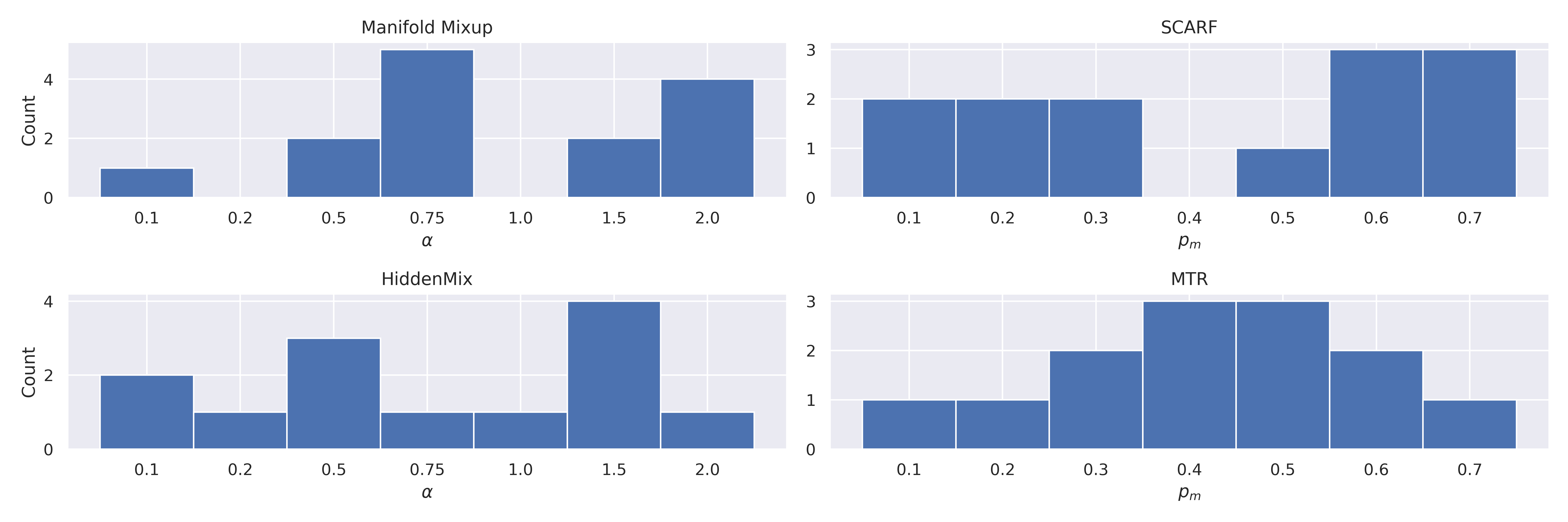
Figure 3: Comparison of hyperparameter distributions for different data augmentation methods in self-supervised learning. The histograms show the aggregated values of the hyperparameters for each of the data augmentation methods for all datasets.

Table 4 shows the results of the self-supervised learning, and Figure 2 shows the distribution of the selected best hyperparameters. Overall, MTR performed the best based on the mean ranks. In particular, it outperformed the other methods on PH dataset. SCARF and HiddenMix also performed better than supervised methods overall, confirming their competitiveness against MTR. Self-supervised learning with Manifold Mixup had the only negative effect. For most of the datasets, the pre-training benefit from self-supervised learning was marginal.

4.3 Ablation study

Table 5: Results for the ablation study in supervised learning. The metrics are averaged over 10 random seeds. For each dataset, the better score is in bold. For each dataset, ranks are computed by sorting the reported scores; the “Rank” column reports the average rank across all datasets.

Dataset JA ↑ SP ↑ PH ↑ WQ ↓ GPS ↑ After bias ($p_{m}$) $\mathbf{85.63}$ (0.6) $\mathbf{98.63}$ (0.7) $\mathbf{82.91}$ (0.7) $\mathbf{0.6804}$ (0.3) $57.55$ (0.2) Before bias ($p_{m}$) $85.50$ (0.7) $98.61$ (0.2) $82.72$ (0.7) $0.6833$ (0.3) $\mathbf{58.34}$ (0.1)

Dataset SH ↑ OS ↑ FI ↓ CA ↓ BM ↑ After bias ($p_{m}$) $\mathbf{86.33}$ (0.5) $92.37$ (0.1) $9779.8$ (0.6) $\mathbf{0.4675}$ (0.4) $\mathbf{93.78}$ (0.6) Before bias ($p_{m}$) $86.31$ (0.4) $\mathbf{92.39}$ (0.1) $\mathbf{9746.2}$ (0.7) $0.4715$ (0.1) $93.75$ (0.3)

Dataset AD ↑ VO ↑ CC ↑ Rank After bias ($p_{m}$) $91.81$ (0.5) $72.06$ (0.1) $98.20$ (0.4) 1.46 Before bias ($p_{m}$) $\mathbf{91.83}$ (0.4) $\mathbf{72.20}$ (0.5) $\mathbf{98.41}$ (0.5) 1.54

In this section, we test design choices of MTR.

Tokenizer in tabular data, including the FT-Transformer’s Tokenizer (Gorishniy et al. (2021) call FeatureTokenizer) used in this experiment, generally consists of weights $W\in\mathbb{R}^{d}$ and biases $b\in\mathbb{R}^{d}$. For example, FeatureTokenizer is defined for the j-th column using $W^{(num)}_{j}\in\mathbb{R}^{d}$ for the numeric column and lookup table $W^{(cat)}_{j}\in\mathbb{R}^{S_{j}\times d}$ for the category column as follows:

$$T^{(num)}_{j}=b^{(num)}_{j}+x^{(num)}_{j}\cdot W^{(num)}_{j} \in\mathbb{R}^{d},$$

$$T^{(cat)}_{j}=b^{(cat)}_{j}+e_{j}^{T}W^{(cat)}_{j} \in\mathbb{R}^{d},$$

$$T=\mathtt{stack}\left[T^{(num)}_{1},\ \ldots,\ T^{(num)}_{k^{(num)}},\ T^{(cat)}_{1},\ \ldots,\ T^{(cat)}_{k^{(cat)}}\right] \in\mathbb{R}^{k\times d}.$$

where $e_{j}^{T}$ is a one-hot vector for the corresponding categorical feature.

We can consider the weights $W$ as directly representing the column value, and the bias $b$ as representing the column itself. Here, our question is whether it is better to apply MTR after bias or before bias. After bias (normal MTR), the subsequent network is not able to recognize the column itself. On the other hand, if MTR is applied before bias, only the column value is masked, and the subsequent network is able to recognize the masked column itself.

Table 5 shows the results of the ablation study in supervised learning. The results are almost the same whether MTR is applied after bias or before bias. Since applying MTR before bias requires modification of the existing Tokenizer, we conclude that applying MTR after bias is superior in terms of implementation cost.

5 Discussion

5.1 When is MTR better than the other data augmentations?

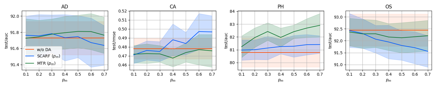
Figure 4: Comparison of SCARF and MTR accuracy variation with mask ratio: SCARF shows significant degradation when a high mask ratio is not suitable, while MTR shows relatively low degradation.

In this section, we discuss scenarios in which MTR outperforms other data augmentation methods.

From Experiment 1, we conclude that MTR is effective for datasets with a large number of features, such as the PH dataset. Such datasets are likely to have high redundancy between columns; MTR hides the information and thus performs well for highly redundant datasets. However, for data with high dependency between columns, it may have a negative impact because necessary information may be lost. For example, in Table 3, we can infer that the value of $p_{m}$ is not suitable for OS and VO datasets with a minimum value of 0.1.

SCARF is sensitive to hyperparameters. Figure 4 compares MTR and SCARF on several datasets; SCARF can be negatively affected by unsuitable hyperparameters, while MTR shows little degradation even at high values of $p_{m}$.

Mixup-family data augmentation requires label-mixing. Multi-modal learning, especially when there are no labels, such as generative models, makes it impossible to use these data augmentations because label-mixing is not applicable.

Based on the above, we conclude that MTR is more suitable than other methods for the following scenarios:

• Training on datasets with redundant columns.

• Training on multi-modal pipelines.

5.2 MTR is like Random Erasing.

Random Erasing (Zhong et al., 2020), data augmentation in the image domain, replaces the pixel value of any patch in the image with a random value from [0, 255]; in the case of ViT (Dosovitskiy et al., 2021), the embedding of a patch replaced by a random value is an irrelevant embedding of the other patches. In the case of MTR, any sequence of embedding is replaced by [mask], which is a learnable parameter shared by all columns and thus becomes a vector unrelated to the unmasked columns. In other words, while Random Erasing in ViT generates irrelevant embedding from meaningless patch, MTR directly replaces them with irrelevant vector [mask]. Thus, MTR can be considered as Random Erasing for tabular data.

5.3 Limitations

Due to the property of MTR to mask information between columns, it may have a negative impact on data with high dependency between columns, since the necessary information may be lost. For example, in Table 3, we can infer that the value of $p_{m}$ is not suitable for the OS and VO datasets with a minimum value of 0.1. In other words, it is likely to not work well for data with a high degree of independence among columns and label values that depend on information in almost all columns. However, using an indicator of the relationship between columns, such as the mutual information content used by Chen et al. (2023), and setting a sort of priority level for the columns to be masked, this negative effect is expected to be reduced.

As we concluded in Section 5.1, MTR is likely to perform relatively well on highly redundant datasets. Highly redundant data is likely to have a large number of columns, but models using the Transformer require more resources for training when the number of columns is large. The main cause of this issue is that the complexity of the vanilla-MHSA (Multi-Head Self-Attention) is quadratic with respect to the number of columns. However, this issue can be alleviated by using an efficient approximation of the MHSA (Tay et al., 2022).

6 Conclusion

This study investigates the status quo in the field of data augmentation for tabular data, which has been important but has not received much attention until now. We performed a fair comparison of each data augmentation method using the same network. We also proposed a novel data augmentation method, MTR, which focuses on the sequence of embedding in Transformer, and showed that it is highly competitive with other data augmentation methods. Furthermore, based on experimental results and the properties of MTR, we provided a scenario in which MTR outperforms other methods. We hope that our work will provide further developments in deep learning for tabular data.

Supplementary material

A Hyperparameters of FTTransformer

We used the default hyperparameters of FTTransformer proposed by Gorishniy et al. [2021] in all experiments. The details of the hyperparameters are shown in Table 6.

Table 6: Default FTTransformer used in the main text. “FFN size factor” is a ratio of the FFN’s hidden size to the feature embedding size. Note that the weight decay is 0.0 for FeatureTokenizer, LayerNorm, and biases.

Layer count	3
Feature embedding size	192
Head count	8
Activation & FFN size factor	(ReGLU, $\nicefrac{{4}}{{3}}$)
Attention dropout	0.2
FFN dropout	0.1
Residual dropout	0.0
Initialization	Kaiming[He et al., 2015]
Optimizer	AdamW
Learning rate	1e-4
Weight decay	1e-5

B Results for all hyperparameters of the experiment

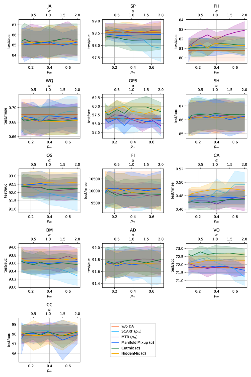
Figure 5: Results for all hyperparameters in Experiment 1. The solid line represents the average score of each method, while the translucent interval indicates the range of standard deviation $\pm\sigma$.

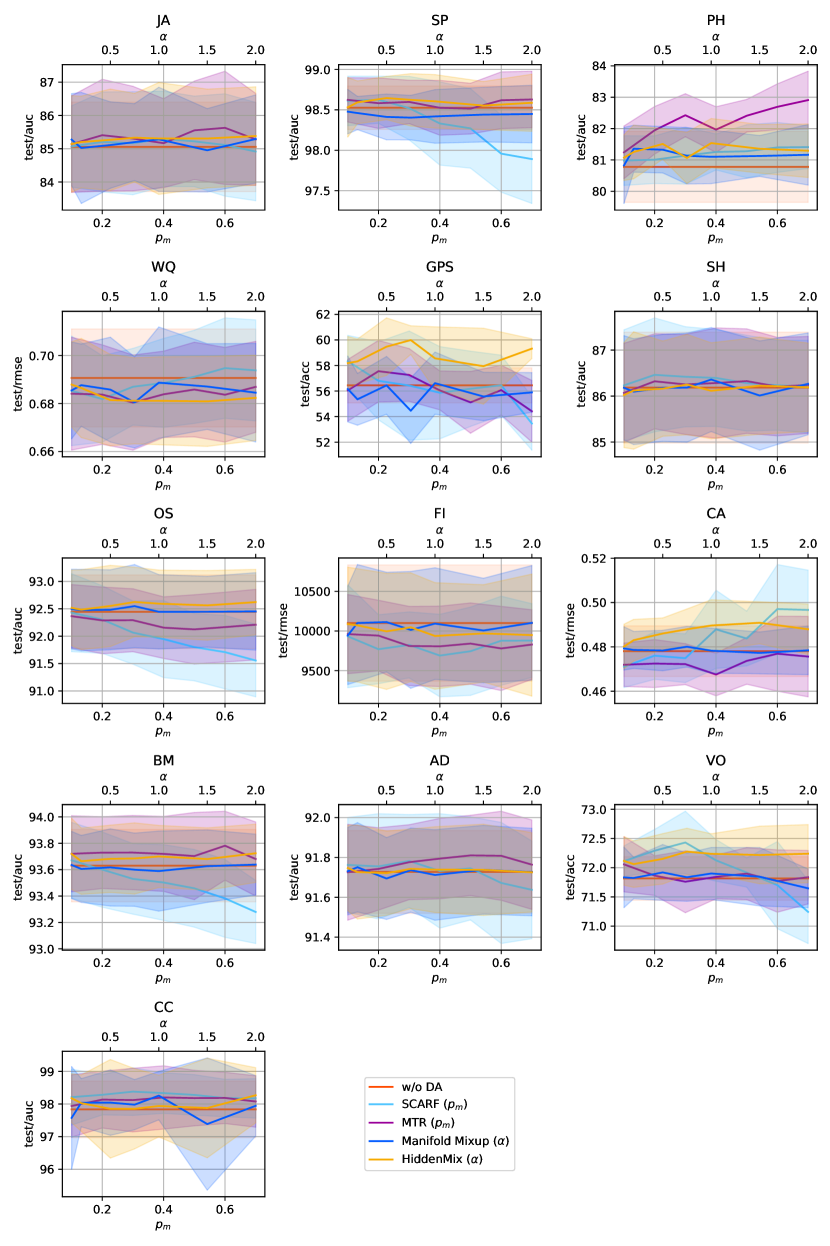
Figure 6: Results for all hyperparameters in Experiment 2. The solid line represents the average score of each method, while the translucent interval indicates the range of standard deviation $\pm\sigma$.

Although we reported only the best hyperparameters in the main text, we provide all the results in this section. The results for all hyperparameters in Experiment 1 are shown in Figure 5, and the results for all hyperparameters in Experiment 2 are shown in Figure 6.

References

- Chen and Guestrin (2016) Tianqi Chen and Carlos Guestrin. Xgboost: A scalable tree boosting system. In Proceedings of the 22nd ACM SIGKDD International Conference on Knowledge Discovery and Data Mining, KDD ’16, page 785–794, New York, NY, USA, 2016. Association for Computing Machinery. ISBN 9781450342322. doi: 10.1145/2939672.2939785. URL https://doi.org/10.1145/2939672.2939785.
- Ke et al. (2017) Guolin Ke, Qi Meng, Thomas Finley, Taifeng Wang, Wei Chen, Weidong Ma, Qiwei Ye, and Tie-Yan Liu. Lightgbm: A highly efficient gradient boosting decision tree. Advances in neural information processing systems, 30, 2017.
- Gorishniy et al. (2021) Yury Gorishniy, Ivan Rubachev, Valentin Khrulkov, and Artem Babenko. Revisiting deep learning models for tabular data, 2021. URL https://arxiv.org/abs/2106.11959.
- Somepalli et al. (2021) Gowthami Somepalli, Micah Goldblum, Avi Schwarzschild, C. Bayan Bruss, and Tom Goldstein. Saint: Improved neural networks for tabular data via row attention and contrastive pre-training. arXiv preprint arXiv:2106.01342, 2021.
- Wang and Sun (2022) Zifeng Wang and Jimeng Sun. TransTab: Learning transferable tabular transformers across tables. In Alice H. Oh, Alekh Agarwal, Danielle Belgrave, and Kyunghyun Cho, editors, Advances in Neural Information Processing Systems, 2022. URL https://openreview.net/forum?id=A1yGs_SWiIi.
- Chen et al. (2023) Jintai Chen, Jiahuan Yan, Danny Ziyi Chen, and Jian Wu. Excelformer: A neural network surpassing gbdts on tabular data, 2023. URL https://arxiv.org/abs/2301.02819.
- Grinsztajn et al. (2022) Léo Grinsztajn, Edouard Oyallon, and Gaël Varoquaux. Why do tree-based models still outperform deep learning on tabular data? arXiv preprint arXiv:2207.08815, 2022.
- Shwartz-Ziv and Armon (2022) Ravid Shwartz-Ziv and Amitai Armon. Tabular data: Deep learning is not all you need. Information Fusion, 81:84–90, 2022.
- Chen et al. (2020) Ting Chen, Simon Kornblith, Mohammad Norouzi, and Geoffrey Hinton. A simple framework for contrastive learning of visual representations. In International conference on machine learning, pages 1597–1607. PMLR, 2020.
- Zhong et al. (2020) Zhun Zhong, Liang Zheng, Guoliang Kang, Shaozi Li, and Yi Yang. Random erasing data augmentation. In Proceedings of the AAAI conference on artificial intelligence, volume 34, pages 13001–13008, 2020.
- Yun et al. (2019) Sangdoo Yun, Dongyoon Han, Seong Joon Oh, Sanghyuk Chun, Junsuk Choe, and Youngjoon Yoo. Cutmix: Regularization strategy to train strong classifiers with localizable features. In Proceedings of the IEEE/CVF International Conference on Computer Vision (ICCV), October 2019.
- Zhang et al. (2017) Hongyi Zhang, Moustapha Cisse, Yann N Dauphin, and David Lopez-Paz. mixup: Beyond empirical risk minimization. arXiv preprint arXiv:1710.09412, 2017.
- Verma et al. (2018) Vikas Verma, Alex Lamb, Christopher Beckham, Amir Najafi, Ioannis Mitliagkas, Aaron Courville, David Lopez-Paz, and Yoshua Bengio. Manifold mixup: Better representations by interpolating hidden states, 2018. URL https://arxiv.org/abs/1806.05236.
- Shorten and Khoshgoftaar (2019) Connor Shorten and Taghi M Khoshgoftaar. A survey on image data augmentation for deep learning. Journal of big data, 6(1):1–48, 2019.
- Feng et al. (2021) Steven Y. Feng, Varun Gangal, Jason Wei, Sarath Chandar, Soroush Vosoughi, Teruko Mitamura, and Eduard Hovy. A survey of data augmentation approaches for nlp, 2021. URL https://arxiv.org/abs/2105.03075.
- Goodfellow et al. (2014) Ian Goodfellow, Jean Pouget-Abadie, Mehdi Mirza, Bing Xu, David Warde-Farley, Sherjil Ozair, Aaron Courville, and Yoshua Bengio. Generative adversarial nets. In Z. Ghahramani, M. Welling, C. Cortes, N. Lawrence, and K.Q. Weinberger, editors, Advances in Neural Information Processing Systems, volume 27. Curran Associates, Inc., 2014. URL https://proceedings.neurips.cc/paper_files/paper/2014/file/5ca3e9b122f61f8f06494c97b1afccf3-Paper.pdf.
- Song et al. (2021) Jiaming Song, Chenlin Meng, and Stefano Ermon. Denoising diffusion implicit models. In International Conference on Learning Representations, 2021. URL https://openreview.net/forum?id=St1giarCHLP.
- Antoniou et al. (2018) Anthreas Antoniou, Amos Storkey, and Harrison Edwards. Data augmentation generative adversarial networks, 2018. URL https://openreview.net/forum?id=S1Auv-WRZ.
- Mariani et al. (2018) Giovanni Mariani, Florian Scheidegger, Roxana Istrate, Costas Bekas, and Cristiano Malossi. Bagan: Data augmentation with balancing gan. arXiv preprint arXiv:1803.09655, 2018.
- Rashid et al. (2019) Haroon Rashid, M Asjid Tanveer, and Hassan Aqeel Khan. Skin lesion classification using gan based data augmentation. In 2019 41st Annual International Conference of the IEEE Engineering in Medicine and Biology Society (EMBC), pages 916–919. IEEE, 2019.
- Bird et al. (2022) Jordan J Bird, Chloe M Barnes, Luis J Manso, Anikó Ekárt, and Diego R Faria. Fruit quality and defect image classification with conditional gan data augmentation. Scientia Horticulturae, 293:110684, 2022.
- Trabucco et al. (2023) Brandon Trabucco, Kyle Doherty, Max Gurinas, and Ruslan Salakhutdinov. Effective data augmentation with diffusion models. In ICLR 2023 Workshop on Mathematical and Empirical Understanding of Foundation Models, 2023. URL https://openreview.net/forum?id=dcCpG0CVMf.
- Azizi et al. (2023) Shekoofeh Azizi, Simon Kornblith, Chitwan Saharia, Mohammad Norouzi, and David J Fleet. Synthetic data from diffusion models improves imagenet classification. arXiv preprint arXiv:2304.08466, 2023.
- Akrout et al. (2023) Mohamed Akrout, Bálint Gyepesi, Péter Holló, Adrienn Poór, Blága Kincső, Stephen Solis, Katrina Cirone, Jeremy Kawahara, Dekker Slade, Latif Abid, et al. Diffusion-based data augmentation for skin disease classification: Impact across original medical datasets to fully synthetic images. arXiv preprint arXiv:2301.04802, 2023.
- Xiao et al. (2023) Changrong Xiao, Sean Xin Xu, and Kunpeng Zhang. Multimodal data augmentation for image captioning using diffusion models. arXiv preprint arXiv:2305.01855, 2023.
- Chawla et al. (2002) Nitesh V Chawla, Kevin W Bowyer, Lawrence O Hall, and W Philip Kegelmeyer. Smote: synthetic minority over-sampling technique. Journal of artificial intelligence research, 16:321–357, 2002.
- Schultz et al. (2023) Kristian Schultz, Waldemar Hahn, Markus Wolfien, Prashant Srivastava, Olaf Wolkenhauer, and Saptarshi Bej. Convgen: A convex space learning approach for deep-generative oversampling and imbalanced classification of small tabular datasets. Available at SSRN 4332129, 2023.
- Engelmann and Lessmann (2021) Justin Engelmann and Stefan Lessmann. Conditional wasserstein gan-based oversampling of tabular data for imbalanced learning. Expert Systems with Applications, 174:114582, 2021.
- Hinton and Salakhutdinov (2006) G. E. Hinton and R. R. Salakhutdinov. Reducing the dimensionality of data with neural networks. Science, 313(5786):504–507, 2006. doi: 10.1126/science.1127647. URL https://www.science.org/doi/abs/10.1126/science.1127647.
- Vincent et al. (2008) Pascal Vincent, Hugo Larochelle, Yoshua Bengio, and Pierre-Antoine Manzagol. Extracting and composing robust features with denoising autoencoders. In Proceedings of the 25th International Conference on Machine Learning, ICML ’08, page 1096–1103, New York, NY, USA, 2008. Association for Computing Machinery. ISBN 9781605582054. doi: 10.1145/1390156.1390294. URL https://doi.org/10.1145/1390156.1390294.
- Yoon et al. (2020) Jinsung Yoon, Yao Zhang, James Jordon, and Mihaela van der Schaar. Vime: Extending the success of self- and semi-supervised learning to tabular domain. In H. Larochelle, M. Ranzato, R. Hadsell, M.F. Balcan, and H. Lin, editors, Advances in Neural Information Processing Systems, volume 33, pages 11033–11043. Curran Associates, Inc., 2020. URL https://proceedings.neurips.cc/paper/2020/file/7d97667a3e056acab9aaf653807b4a03-Paper.pdf.
- Majmundar et al. (2022) Kushal Majmundar, Sachin Goyal, Praneeth Netrapalli, and Prateek Jain. Met: Masked encoding for tabular data, 2022.
- Onishi et al. (2023) Soma Onishi, Kenta Oono, and Kohei Hayashi. Tabret: Pre-training transformer-based tabular models for unseen columns. In ICLR 2023 Workshop on Mathematical and Empirical Understanding of Foundation Models, 2023. URL https://openreview.net/forum?id=qnRlh8BdMY.
- Bahri et al. (2022) Dara Bahri, Heinrich Jiang, Yi Tay, and Donald Metzler. Scarf: Self-supervised contrastive learning using random feature corruption. In International Conference on Learning Representations, 2022. URL https://openreview.net/forum?id=CuV_qYkmKb3.
- Ucar et al. (2021) Talip Ucar, Ehsan Hajiramezanali, and Lindsay Edwards. Subtab: Subsetting features of tabular data for self-supervised representation learning. Advances in Neural Information Processing Systems, 34:18853–18865, 2021.
- Darabi et al. (2021) Sajad Darabi, Shayan Fazeli, Ali Pazoki, Sriram Sankararaman, and Majid Sarrafzadeh. Contrastive mixup: Self- and semi-supervised learning for tabular domain, 2021. URL https://arxiv.org/abs/2108.12296.
- Hajiramezanali et al. (2022) Ehsan Hajiramezanali, Nathaniel Lee Diamant, Gabriele Scalia, and Max W Shen. STab: Self-supervised learning for tabular data. In NeurIPS 2022 First Table Representation Workshop, 2022. URL https://openreview.net/forum?id=EfR55bFcrcI.
- Chen and He (2021) Xinlei Chen and Kaiming He. Exploring simple siamese representation learning. In 2021 IEEE/CVF Conference on Computer Vision and Pattern Recognition (CVPR), pages 15745–15753, 2021. doi: 10.1109/CVPR46437.2021.01549.
- Vaswani et al. (2017) Ashish Vaswani, Noam Shazeer, Niki Parmar, Jakob Uszkoreit, Llion Jones, Aidan N. Gomez, Lukasz Kaiser, and Illia Polosukhin. Attention is all you need, 2017.
- Devlin et al. (2019) Jacob Devlin, Ming-Wei Chang, Kenton Lee, and Kristina Toutanova. BERT: Pre-training of deep bidirectional transformers for language understanding. In Proceedings of the 2019 Conference of the North American Chapter of the Association for Computational Linguistics: Human Language Technologies, Volume 1 (Long and Short Papers), pages 4171–4186, Minneapolis, Minnesota, June 2019. Association for Computational Linguistics. doi: 10.18653/v1/N19-1423. URL https://aclanthology.org/N19-1423.
- Guyon et al. (2019) Isabelle Guyon, Lisheng Sun-Hosoya, Marc Boullé, Hugo Jair Escalante, Sergio Escalera, Zhengying Liu, Damir Jajetic, Bisakha Ray, Mehreen Saeed, Michèle Sebag, et al. Analysis of the automl challenge series. Automated Machine Learning, 177, 2019.
- Dua and Graff (2017) Dheeru Dua and Casey Graff. UCI machine learning repository, 2017. URL http://archive.ics.uci.edu/ml.
- Cortez et al. (2009) Paulo Cortez, António Cerdeira, Fernando Almeida, Telmo Matos, and José Reis. Modeling wine preferences by data mining from physicochemical properties. Decision Support Systems, 47(4):547–553, 2009. ISSN 0167-9236. doi: https://doi.org/10.1016/j.dss.2009.05.016. URL https://www.sciencedirect.com/science/article/pii/S0167923609001377. Smart Business Networks: Concepts and Empirical Evidence.
- Sakar et al. (2019) C. Okan Sakar, S. Polat, Mete Katircioglu, and Yomi Kastro. Real-time prediction of online shoppers’ purchasing intention using multilayer perceptron and lstm recurrent neural networks. Neural Computing and Applications, 31, 10 2019. doi: 10.1007/s00521-018-3523-0.
- Pace and Barry (1997) Kelley Pace and Ronald Barry. Sparse spatial autoregressions. Statistics & Probability Letters, 33(3):291–297, 1997. URL https://EconPapers.repec.org/RePEc:eee:stapro:v:33:y:1997:i:3:p:291-297.
- Moro et al. (2014) Sérgio Moro, Paulo Cortez, and Paulo Rita. A data-driven approach to predict the success of bank telemarketing. Decision Support Systems, 62:22–31, 2014. ISSN 0167-9236. doi: https://doi.org/10.1016/j.dss.2014.03.001. URL https://www.sciencedirect.com/science/article/pii/S016792361400061X.
- Kohavi (1996) Ron Kohavi. Scaling up the accuracy of naive-bayes classifiers: a decision-tree hybrid. In Proceedings of the Second International Conference on Knowledge Discovery and Data Mining, page to appear, 1996.
- Pozzolo et al. (2015) Andrea Dal Pozzolo, Olivier Caelen, Reid A. Johnson, and Gianluca Bontempi. Calibrating probability with undersampling for unbalanced classification. In 2015 IEEE Symposium Series on Computational Intelligence, pages 159–166, 2015. doi: 10.1109/SSCI.2015.33.
- Pedregosa et al. (2011) F. Pedregosa, G. Varoquaux, A. Gramfort, V. Michel, B. Thirion, O. Grisel, M. Blondel, P. Prettenhofer, R. Weiss, V. Dubourg, J. Vanderplas, A. Passos, D. Cournapeau, M. Brucher, M. Perrot, and E. Duchesnay. Scikit-learn: Machine learning in Python. Journal of Machine Learning Research, 12:2825–2830, 2011. URL http://www.jmlr.org/papers/volume12/pedregosa11a/pedregosa11a.pdf.
- Dosovitskiy et al. (2021) Alexey Dosovitskiy, Lucas Beyer, Alexander Kolesnikov, Dirk Weissenborn, Xiaohua Zhai, Thomas Unterthiner, Mostafa Dehghani, Matthias Minderer, Georg Heigold, Sylvain Gelly, Jakob Uszkoreit, and Neil Houlsby. An image is worth 16x16 words: Transformers for image recognition at scale. In International Conference on Learning Representations, 2021. URL https://openreview.net/forum?id=YicbFdNTTy.
- Tay et al. (2022) Yi Tay, Mostafa Dehghani, Dara Bahri, and Donald Metzler. Efficient transformers: A survey. ACM Computing Surveys, 55(6):1–28, 2022.
- He et al. (2015) Kaiming He, Xiangyu Zhang, Shaoqing Ren, and Jian Sun. Delving deep into rectifiers: Surpassing human-level performance on imagenet classification. In Proceedings of the IEEE international conference on computer vision, pages 1026–1034, 2015.