Heterogeneous Noise and Stable Miscoordination

Abstract

Coordination games admit two types of equilibria: pure equilibria, where all players successfully coordinate their actions, and mixed equilibria, where players frequently experience miscoordination. The existing literature shows that under many evolutionary dynamics, populations converge to a pure equilibrium from almost any initial distribution of actions. By contrast, we show that under plausible learning dynamics, where agents observe the actions of a random sample of their opponents and adjust their strategies accordingly, stable miscoordination can arise when there is heterogeneity in the sample sizes. This occurs when some agents make decisions based on small samples (anecdotal evidence) while others rely on large samples. Finally, we demonstrate the empirical relevance of our results in a bargaining application.

Keywords: sampling best response dynamics, action-sampling dynamics, coordination games, hawk-dove games, evolutionary stability, logit dynamics.     JEL Classification: C72, C73.

1 Introduction

Many real-life situations can be modeled as coordination games, in which the best response against an opponent’s action is to play the same action (possibly after relabeling the actions of one of the players). Two-player, two-action coordination games admit three equilibria of two distinct types: two strict pure equilibria, where the players successfully coordinate their actions, and a mixed equilibrium, where players frequently experience miscoordination. A fundamental result in evolutionary game theory is that under a broad set of learning dynamics, the mixed equilibrium is unstable and populations in which agents are randomly matched to play coordination games must converge to everyone playing one of the pure equilibria (as surveyed in Section 2). By contrast, in this paper we show that the mixed equilibrium with miscoordination can be stable if the populations are heterogeneous in the sense that some (but not all) of the agents rely on anecdotal evidence induced by small samples.

Highlights of the Model

Consider a setup in which pairs of agents from two infinite populations are repeatedly randomly matched to play a (one-shot) coordination game. Agents occasionally die and are replaced by new agents (or, alternatively, agents occasionally receive opportunities to revise their actions). The new agents do not have precise information about the aggregate behavior in the opponent’s population, and estimate this from sampling the opponent’s population. Specifically, each population $i$ is characterized by a distribution of sample sizes $\theta_{i}$, such that $\theta_{i}\left(k\right)$ is the frequency of agents with sample size $k$. Each such agent observes the behavior of $k$ random opponents, and then adopts the action that is a best response to her sample (with an arbitrary tie-breaking rule).

These learning dynamics, which seem plausible in various setups, are called sampling best-response dynamics (Sandholm, 2001; Osborne and Rubinstein, 2003; Oyama, Sandholm, and Tercieux, 2015, henceforth abbreviated as sampling dynamics).

As explained in Appendix A.1, any two-action coordination game (such as the battle of the sexes or the stag hunt) can be represented w.l.o.g. by the payoff matrix presented in Table 1 that has two positive parameters $\left(u_{1},u_{2}\right)$ that represent the players’ payoffs when both play the first action: the payoffs when coordinating on the second action are normalized to 1, and the payoffs for miscoordinating are normalized to 0.

Table 1: Standard Representation of Two-Action Coordination Game

	$a_{2}$	$b_{2}$
$~{}~{}a_{1}~{}~{}$	$\,\,{}_{\underset{\,}{{\color[rgb]{0,0,1}u_{1}}}}{\,{}^{\overset{\,}{u_{2}}}}$	${{}_{\underset{\,}{0}}}\,\,^{{\color[rgb]{180,00,00}\overset{\,}{0}}}$
$~{}~{}b_{1}~{}~{}$	${}_{\underset{\,}{{\color[rgb]{0,0,1}0}}}\,\,^{\overset{\,}{{\color[rgb]{180,00,00}0}}}$	${}_{{\color[rgb]{0,0,1}1}}\,\,\,\,^{{\color[rgb]{180,00,00}1}}$

The following definition will be helpful for presenting our results. An action is $q$-dominant (Morris, Rob, and Shin, 1995) to player $i$ if it is the player’s best response against any opponent’s mixed action that assigns a mass of at least $q$ to the opponent playing the same action. In particular, action $a_{i}$ (resp., $b_{i}$) is $\frac{1}{2}$-dominant for player $i$ if it is the best response against an opponent’s uniform play, which is the case iff $u_{i}>1$ (resp., $u_{i}<1$).

Global Convergence to Miscoordination

Theorem 1 presents a full characterization for environments in which the populations converge to states with miscoordination from almost all initial states. This happens if (and essentially only if): (1) each population has a different $\frac{1}{2}$-dominant action (i.e., $u_{2}<1<u_{1}$), (2) the product of the mass of agents with sample size 1 times the expected sample size of the other population is larger than one (i.e., $\forall i,\,\,\theta_{i}\left(1\right)\cdot\mathbb{E}\left(\theta_{j}\right)>1$ ), and (3) each population has a $q$-dominant action for a sufficiently low $q$ (which is satisfied iff each $u_{i}$ is sufficiently far from 1).

The proof idea is as follows. Global convergence to miscoordination occurs iff both pure equilibria are unstable. Assume that $u_{2}<1<u_{1}$. Consider a slightly perturbed state near the equilibrium $\left(a_{1},a_{2}\right)$, in which $\epsilon_{i}<<1$ of the agents in population $i$ plays $b_{i}$. Events in which a new agent observes multiple occurrences of the opponent’s rare action $b_{j}$ in her sample are negligible ($O\left(\epsilon_{j}^{2}\right)$). Neglecting these very rare events implies that new agents of population $1$ will adopt the risk-dominated action $b_{1}$ only when they have sample size 1, and they have observed the rare action $b_{2}$ (the probability of this is $\theta_{1}\left(1\right)\cdot\epsilon_{2}$). By contrast, if $u_{2}<1$ is sufficiently small, then a single occurrence of the rare action $b_{1}$ in a sample of size $k$ (which occurs with probability of $k\cdot\epsilon_{1}$) is sufficient to induce a new agent of population 2 to play her $\frac{1}{2}$-dominant action $b_{2}$. This implies that the total share of new agents of population 2 who play action $b_{2}$ is $\mathbb{E}\left(\theta_{2}\right)\cdot\epsilon_{1}$. This, in turn, implies that the product of the number of agents playing the rare action in each population increases iff $\theta_{1}\left(1\right)\cdot\mathbb{E}\left(\theta_{2}\right)>1$.

Heterogeneity and Stable Miscoordination

Our second main result (Theorem 2) shows that heterogeneity in the sample sizes is necessary for stable miscoordination. Specifically, we show that if all agents in each population $i$ have the same sample size $k_{i}\geq 2$, then all states with miscoordination are unstable (the case in which everyone has sample size 1 is discussed in Remark 1). Our final result (Theorem 3) shows that many heterogeneous distributions of sample sizes in which some agents have relatively small samples and others have sufficiently large samples induce locally stable states with miscoordination if $u_{1}$ and $u_{2}$ are not too close to 1.

The intuition for why heterogeneity in the sample sizes is important for the stability of interior states with miscoordination is as follows. Consider homogeneous populations with a fixed sample size $k$ in a stationary interior state. In such a state the random sample of size $k$ frequently yields both outcomes for which action $a_{i}$ is a best response and outcomes for which $b_{i}$ is a best response. We show that in such situations the probability of each action being a best response is sensitive to small perturbations in the opponent’s distribution of actions. That is, if $\epsilon$ more of the opponent’s population play $a_{j}$, it increases the probability that $a_{i}$ is the best response to the random sample by more than $\epsilon$.

Next consider a heterogeneous population in which some agents have relatively small samples, while other agent have large samples. The stationary interior state with miscoordination typically does not coincide with the mixed Nash equilibrium, which implies that almost all agents with large samples play the same action (the unique best response to the true distribution of the opponents’ actions), and that their play is insensitive to small perturbations of the opponents’ behavior. This allows the overall sensitivity of the entire population to small perturbations to be sufficiently small to allow stable miscoordination.

Theorem 2’s proof relies on deriving a property of binomial distributions (Proposition 3), which may be of independent interest. This property states that a composition of two binomial cumulative distributions has a unique interior fixed point.

Numerical Analysis and Insights

In Section 7 we demonstrate our main insight that heterogeneity in the sample sizes induces stable miscoordination does not depend on the specific details of the sampling dynamics. Specifically, we numerically study the commonly used logit dynamics, in which agents play a noisy best response to their opponents’ aggregate behavior, with $\eta_{i}$ describing the noise level in population $i$. We first demonstrate that if the noise level in each population is homogeneous, then one can induce stable miscoordination only with implausibly high levels of noise. By contrast, when we introduce an extension of logit dynamics that allows heterogeneity in the level of noise in each population, we show that stable miscoordination can be supported by moderate heterogeneous levels of noise.

Taken together, our results show that the conventional wisdom that miscoordination is unstable is not accurate. Miscoordination can be stable in heterogeneous populations in which some agents rely on anecdotal evidence or noisy data, while other agents have access to more accurate data. The experimentally testable implications of our results are discussed in Section 2.

Bargaining Application and Empirical Relevance

Demonstrating the empirical relevance of our theoretical findings requires real-life scenarios in which it is plausible to have: (1) heterogeneous sample sizes, (2) persistent miscoordination within an interior state, and (3) a substantial proportion of agents not maximizing their payoffs with respect to the aggregate behavior of the other population. We argue that these conditions might exist in bargaining situations in both housing and used-car markets. Coordination games can model simple bargaining in these markets, where each agent has two strategies: a high-price strategy or low-price strategy. For example, a seller can either demand a high price (with the risk of bargaining failure) or agree to a low price, and a buyer can either agree to a high price or insist on a low price (as modeled by hawk-dove coordination games; see Example 3 in Appendix A.1). Heterogeneity in the sample sizes is likely to exist in these markets, where both professional players (real-estate investors and car dealers) and inexperienced players (those who have only bought or sold houses or cars a couple of times) participate. Professional players are likely to have access to large samples, while inexperienced players may rely on anecdotal evidence.

Koster and Rouwendal (2021) conducted an empirical study on the Dutch housing market. They found that a significant number of sellers set low list prices, which can be consistent with profit maximization only if the sellers have high annual discount factors of up to 50%. This behavior is consistent with an interior stable state in our model in which some sellers rely on small, noisy samples to choose non-payoff-maximizing low prices. Koster and Rouwendal’s data does not allow separating between different types of sellers. By contrast, Genesove and Mayer (2001) does allow separating the sellers to owner-occupants and investors, and show that the two groups have systematic differences in their list prices.

Larsen (2021) empirically studied the efficiency of bargaining following wholesale used-car auctions in which the highest bid is lower than the reserve price, and found that bargaining fails in about 35% of these cases (which is consistent with an interior stable state with miscoordination). The data suggests that this inefficiency results in substantial losses, representing 12%-23% of ex-post gains from trade. Furthermore, Larsen’s analysis suggests that only a small part of this loss is due to incomplete information constraints.

Structure

Section 2 presents the related literature. Our model is described in Section 3. Section 4 presents a “complete” characterization of global convergence to states with miscoordination. In Section 5, we show that homogeneous populations always converge to one of the pure equilibria. Section 6 shows that many heterogeneous populations can induce locally stable states with miscoordination. In Section 7, we numerically analyze logit dynamics, and demonstrate that our main insights hold in this setup as well. We conclude in Section 8. Formal proofs and additional results are presented in the appendix. Appendix A.2 extends our results to one-population dynamics. Appendix A.3 states and proves an interesting general result on binomial distributions.

2 Related Literature

Instability of Miscoordination

It is well-known that strict equilibria satisfy strong stability refinements, while mixed equilibria with miscoordination do not satisfy even weak stability refinements. In particular, strict equilibria are evolutionarily stable (Maynard Smith and Price, 1973), while the mixed equilibrium does not satisfy neutral stability (Maynard Smith, 1982) or even the mild refinement of weak stability (Heller, 2017). Moreover, it is well known that interior stationary states in all multiple-population games cannot be asymptotically stable under the widely studied replicator dynamics (see, e.g., Sandholm, 2010, Theorem 9.1.6). Instability of interior states is further shown for various classes of learning dynamics in Crawford (1989).

Moreover, various papers in the literature have proven that populations playing coordination games converge to one of the pure equilibria from almost all initial states under various dynamics. Kaniovski and Young (1995) show that there is global convergence to one of the pure equilibria for sampling dynamics with sufficiently large samples. Oprea, Henwood, and Friedman (2011) show that there is global convergence to one of the pure equilibria under monotone dynamics (i.e., under any dynamics in which an action becomes more frequent iff it yields a higher payoff than the alternative action). Recently, Oyama, Sandholm, and Tercieux (2015) proved the global stability of the $\frac{1}{2}$-dominant pure equilibrium in symmetric coordination games for distributions of sample sizes in which sufficiently many agents have sufficiently small samples. The stochastic evolutionary dynamics literature (pioneered by Kandori, Mailath, and Rob, 1993; Young, 1993; see also the recent application to hawk-dove games in Bilancini, Boncinelli, Ille, and Vicario, 2022) shows that only pure equilibria can be stochastically stable in large finite populations in which agents most of the time best respond to a large sample, but occasionally mistakenly play the other action.

Thus, taken together, the various existing studies suggest that states with miscoordination are unstable. Our contribution is in showing that this is not the case in plausible learning dynamics in which agents base their behavior on sampling the actions of the other population, and there is substantial heterogeneity in the sample sizes in each population.

Sampling Dynamics

Sampling best-response dynamics (henceforth, sampling dynamics) were pioneered by Sandholm (2001) and Osborne and Rubinstein (2003). As argued by Oyama, Sandholm, and Tercieux (2015), the deterministic nature of sampling dynamics implies that when there is convergence to a stable state (which is always the case in our setup; see Proposition 2) the convergence is fast. Recently, Heller and Mohlin (2018) studied the conditions on the expected sample size that implies global convergence for all payoff functions and all sampling dynamics.

Salant and Cherry (2020) (see also Sawa and Wu, 2023) generalized sampling dynamics by allowing new agents to use various procedures to infer from their samples the aggregate behavior of the opponents (in addition to allowing for payoff heterogeneity in the population). Salant and Cherry paid special attention to unbiased inference procedures in which the agent’s expected belief about the share of opponents who play an action coincides with the sample mean. Examples of unbiased procedures are maximum likelihood estimation, beta estimation with a prior representing complete ignorance, and a truncated normal posterior around the sample mean. In our setup, the payoffs are linear in the share of agents who play action $a_{j}$, which implies that the agent’s perceived best response depends only on the expectation of her posterior belief. This implies that the behavior of agents in our model can be interpreted as each new agent utilizes her own sample to calculate an unbiased estimation procedure (such as, maximum likelihood estimation) for the overall behavior of the opposing population. remains the same with any unbiased inference procedure.

Experimental Literature and Testable Predictions

Our model yields a novel testable prediction: miscoordination can persist when there is heterogeneity in the amount of information that the agents have about the opponents’ behavior, and for each population one of the actions is $q$-dominant for a sufficiently low $q$. Brunner, Camerer, and Goeree (2011) compared the predictive power of various learning models when applied to the experimental data of McKelvey, Palfrey, and Weber (2000), Goeree, Holt, and Palfrey (2003), and Selten and Chmura (2008), in which (1) agents are randomly and repeatedly matched to play a one-shot two-action two-player game against an anonymous opponent, and (2) agents get feedback only about their most recent opponent’s play (and can rely on their memory of her previous feedback about past opponents). Brunner, Camerer, and Goeree’s findings show that sampling dynamics explain well the aggregate experimental behavior, and that sampling dynamics’ predictions are: (1) as good as the quantal response equilibrium in all games and significantly better in some games, (2) significantly better than the Nash equilibrium in all games, and (3) significantly improve when focusing on the less noisy second halves of the treatments (see, Brunner, Camerer, and Goeree, 2011, Figure 4).

Brunner, Camerer, and Goeree’s results suggest that sample sizes of 3–12 fit the data best (which is roughly in line with the typical estimates of people’s short-run memory capacity). The prediction of global convergence to miscoordination (Theorem 1) requires that a substantial part of the population to have a small sample size of 1. This may be induced by having some subjects playing in different rounds different underlying games. For example, in each round, one of several underlying games will be played. Each subject will be informed about the payoff matrix of the current game, and will be reminded about her most recent past opponent’s behavior in the previous period in which the same game was played. It seems plausible that many subjects will rely only on this feedback when deciding how to play (i.e., essentially have a sample of size 1), while only a few subjects will exert effort to remember relevant past feedback from less recent periods in which the same game was played.

Recently, Lyu, Li, and Xu (2022) applied a more elaborate experimental setup that aims to implement sampling dynamics. In their implementation the subjects are endowed with a specific “default” action to play in the first round. This novel design component allows us to test dynamic predictions with respect to specific initial states. At the end of each round each agent observes the $k$ most recent actions ($k=2$ and $k=7$ were applied in their treatments) of random opponents among the 14 players in their matching group. Their underlying games were symmetric coordination games with Pareto-ranked pure equilibria. Lyu, Li, and Xu showed that action-sampling dynamics (with respect to the most recent $k$ observed actions) fits about 80% of the subjects’ behavior.

A central reason why some subjects deviated from the predictions of sampling dynamics (especially in early rounds) was that they played the action that is part of the Pareto-dominant equilibrium in order to “teach” the other subjects in the matching group to move from the Pareto-dominated equilibrium to the Pareto-dominant equilibrium. These “teaching” incentives were justified, as they often helped groups starting in the Pareto-dominated equilibrium to shift to the Pareto-dominant equilibrium. We think that “teaching”incentives would be substantially reduced, and the fit of sampling dynamics would be substantially improved, if either (1) the strict equilibria of the underlying coordination games were not Pareto-ranked (e.g., battle of the sexes), or (2) the matching groups were substantially larger.

The predictions of Theorem 3 (local stability of miscoordination) require both an appropriate initial state (which can be implemented $\grave{\textrm{a}}$ la Lyu, Li, and Xu, 2022), and that some agents will have accurate information about the opponents’ aggregate behavior. This can be implemented by providing some agents with full feedback about the behavior of all opponents in the previous round (while providing the remaining agents with feedback about the behavior of only their own matched opponents).

3 Model

3.1 Coordination Games

Let $G=\{A_{1}\times A_{2},u\}$ denote a normal-form two-action two-player coordination game. Let $i\in\left\{1,2\right\}$ be an index denoting one of the players (“she”), and let $j$ denote her opponent (“he”). For each $i\in\left\{1,2\right\}$, let $A_{i}=\left\{a_{i},b_{i}\right\}$ denote the actions of player $i$.

The standard two-parameter payoff matrix of a coordination game is given in Table 2: the players get a low payoff (normalized to 0) if they miscoordinate (i.e., one player plays $a_{i}$ and the opponent plays $b_{j}$), they get a high payoff (normalized to 1) if they coordinate on both playing $\left(b_{1},b_{2}\right)$, and they get a payoff of $u_{i}>0$ if they coordinate on both playing $\left(a_{1},a_{2}\right)$. By relabeling the actions we can assume w.l.o.g. that action profile a is the weakly preferred outcome of Player 1; i.e., we assume that $u_{1}\geq 1.$ We say that the coordination game is (1) symmetric if $u_{1}=u_{2}$, and (2) antisymmetric if $u_{1}=\frac{1}{u_{2}}.$ Antisymmetric coordination games can be interpreted as battle of the sexes games, in which Player 1’s preference for the first coordinated outcome a over the second coordinated outcome b is as strong as Player 2’s preference for b over a.

In Appendix A.1 we formally show that this standard two-parameter representation captures w.l.o.g. two-action coordination games (including battle of the sexes, stag hunt, and hawk-dove games). This is so because our dynamics (as defined in Eq. (3.1) and Eq. (A.1))) depend only on the differences between the payoffs of a player in action profiles in which the opponent plays the same action. This implies that the dynamics are invariant to (1) adding a constant to the two payoffs of Player 1 (resp., Player 2) in the same row (resp., column), and (2) dividing all the payoffs of a player by a positive constant.

We extend the game to mixed actions in the standard linear way. We identify each mixed action with the probability it assigns to the first action ($a_{i}$), and we denote it by $p_{i}\in\left[0,1\right]$. We identify the degenerate mixed action $1$ (resp., $0$) with the pure action $a_{i}$ (resp., $b_{i}$). Observe that the coordination game admits three Nash equilibria: two pure equilibria, $\left(a_{1},a_{2}\right)$ and $\left(b_{1},b_{2}\right),$ in which the players coordinate their actions, and a mixed equilibrium $\boldsymbol{p}^{NE}=\left(\frac{1}{1+u_{2}},\frac{1}{1+u_{1}}\right)$ in which the players frequently experience miscoordination.

Table 2: Standard Representation of Two-Action Coordination Game

	$a_{2}$	$b_{2}$
$~{}~{}a_{1}~{}~{}$	$\,\,{}_{\underset{\,}{{\color[rgb]{0,0,1}u_{1}}}}{\,{}^{\overset{\,}{u_{2}}}}$	${{}_{\underset{\,}{0}}}\,\,^{{\color[rgb]{180,00,00}\overset{\,}{0}}}$
$~{}~{}b_{1}~{}~{}$	${}_{\underset{\,}{{\color[rgb]{0,0,1}0}}}\,\,^{\overset{\,}{{\color[rgb]{180,00,00}0}}}$	${}_{{\color[rgb]{0,0,1}1}}\,\,\,\,^{{\color[rgb]{180,00,00}1}}$
$\underset{\,}{{\color[rgb]{0,0,1}u_{1}\geq 1}}$, $u_{2}$>0

$\frac{1}{2}$-Dominance

Fix $q\in\left[0,1\right]$. We say that action $a_{i}$ (resp., $b_{i}$) is $q$-dominant (Morris, Rob, and Shin, 1995; Oyama, Sandholm, and Tercieux, 2015) for player $i$ if it is a strict best response to any opponent’s mixed action that assigns a mass of at least $q$ to the counterpart action $a_{j}$ (resp., $b_{j}$).

Notice that both actions are 1-dominant (which is equivalent to being part of a strict equilibrium). Additionally, it can be noted that as $q$ decreases, the $q$-dominance condition becomes more stringent. In other words, if an action is $q$-dominant, it also satisfies $r$-dominance for any $q$ between $r$ and 1. Lastly, it can be observed that action $a_{i}$ is $\frac{1}{1+u_{i}}$-dominant, while action $b_{i}$ is $\frac{u_{i}}{1+u_{i}}$-dominant.

We say that the pure equilibrium a (resp., b) is $\frac{1}{2}$-dominant if each action $a_{i}$ (resp., $b_{i}$) is $\frac{1}{2}$-dominant; in this case we say that the remaining equilibrium is risk dominated. Observe that the game admits a $\frac{1}{2}$-dominant equilibrium iff $u_{1},u_{2}>1$. By contrast, if $u_{1}>1>u_{2}$, then $a_{1}$ is $\frac{1}{2}$-dominant for player 1 and $b_{2}$ is $\frac{1}{2}$-dominant for player 2.

Observe that $q$-dominance depends only on the differences between the payoffs a player can get by playing the different actions. This implies that $q$-dominance is invariant to both of the payoff transformations mentioned above (and described in detail in Appendix A.1). This implies that an action is $q$-dominant in the standard representation of Table 2 iff it is $q$-dominant in the original representation as a general coordination game (as described in Appendix A.1). By contrast, payoff dominance is not invariant to the first of these two transformations. Specifically, adding a constant to the two payoffs of Player 1 (Player 2) in the same row (column) might change a Pareto-dominated equilibrium into a Pareto-dominant equilibrium.

3.2 Evolutionary Dynamics

We assume that there are two unit-mass continuums of agents and that agents in population 1 are randomly matched with agents in population 2. Aggregate behavior at time $t\in\mathbb{R}^{+}$ is described by a state $\mathbf{p}\left(t\right)=\left(p_{1}\left(t\right),p_{2}\left(t\right)\right)\in\left[0,1\right]^{2}$, which is equivalent to a mixed action profile (i.e., $p_{i}\left(t\right)$ represents the share of agents playing action $a_{i}$ at time $t$ in population $i$). A state $\mathbf{p}=\left(p_{1},p_{2}\right)$ is interior (i.e., mixed) if $p_{1},p_{2}\in(0,1).$

Agents die at a constant rate of 1, and are replaced by new agents (or, equivalently, agents get opportunities to revise their actions). The evolutionary process is represented by a function $\textbf{w}:\left[0,1\right]^{2}\rightarrow\left[0,1\right]^{2}$, which describes the frequency of new agents in each population who play action $a_{i}$ as a function of the current state. Thus, the instantaneous change in the share of agents in population $i$ who play $a_{i}$ is given by the following dynamics (where $w_{i}$ is as defined in Eq. (A.1) below):

$$\dot{p}_{i}=w_{i}\left(p_{j}\right)-p_{i}.$$ (3.1)

Sample Sizes

We allow heterogeneity in the sample sizes used by new agents. Let $\theta_{i}\in\Delta\left(\mathbb{Z}_{+}\right)$ denote the distribution of sample sizes of new agents in population $i$. We assume that $\theta_{i}$ has a finite support. A share of $\theta_{i}\left(k\right)$ of the new agents have a sample of size $k$. Let $\text{supp}\left(\theta_{i}\right)$ denote the support of $\theta_{i}$. If there exists some $k,$ for which $\theta_{i}(k)=1,$ then we use $k$ to denote the degenerate (homogeneous) distribution $\theta_{i}\equiv k$.

Remark 1.

We assume that some agents have sample sizes larger than 1 (i.e., $\forall i$
$\max(\textrm{supp}(\theta_{i}))>1$). This rules out the trivial case in which all agents have sample size 1. In this case, the entire diagonal $\left\{\left(p,p\right)|p\in\left[0,1\right]\right\}$ is Lyapunov stable, and no state is asymptotically stable (as shown in Sethi, 2000, Example 7 in a related setup).

Definition 1.

An environment is a tuple $\left(\boldsymbol{u},\boldsymbol{\theta}\right)=\left(\left(u_{1},u_{2}\right),\left(\theta_{1},\theta_{2}\right)\right)$, where $\left(u_{1},u_{2}\right)$ describe the payoffs of the underlying coordination game, and $\left(\theta_{1},\theta_{2}\right)$ describes the distributions of sample sizes in each population.

Sampling Best-Response Dynamics

Sampling best-response dynamics (henceforth sampling dynamics; Sandholm, 2001; Oyama, Sandholm, and Tercieux, 2015 ) fit situations in which agents do not know the exact distribution of actions in the other population. New agents estimate this unknown distribution by sampling the opponent’s actions. Specifically, each new agent with sample size $k$ (henceforth, $k$-agent) samples $k$ randomly drawn agents from the other population and then plays the action that is the best response against the sample. One possible interpretation of this behavior is that each new agent utilizes her own sample to calculate a maximum likelihood estimation for the overall behavior of the opposing population (or by any other unbiased estimation procedure, $\grave{\textrm{a}}$ la Salant and Cherry, 2020).

To simplify notation, we assume that in case of the tie, the new agent plays $a_{i}$. Our results are essentially the same for any tie-breaking rule.

Let $X(k,p_{j})\sim Bin\left(k,p_{j}\right)$ denote a random variable with binomial distribution with parameters $k$ (number of trials) and $p_{j}$ (probability of success in each trial), which is interpreted as the number of $a_{j}$-s in the sample. Observe that the sum of payoffs of playing action $a_{i}$ against the sample is $u_{i}\cdot X(k,p_{j})$ and the sum of payoffs of playing action $b_{i}$ against the sample is $k-X(k,p_{j})$.

This implies that action $a_{i}$ is a best response to a sample of size $k$ iff $u_{i}\cdot X(k,p_{j})\geq k-X(k,p_{j})\Leftrightarrow X(k,p_{j})\geq\frac{k}{u_{i}+1}$. This, in turn, implies that the sampling dynamics for environment $\left(\boldsymbol{u},\boldsymbol{\theta}\right)$ is given by

$$w_{i}\left(p_{j}\right)=\sum_{k\in\text{supp}\left(\theta_{i}\right)}\theta_{i}(k)\cdot\Pr\left(X\left(k,p_{j}\right)\geq\frac{k}{u_{i}+1}\right).$$ (3.2)

Observe that $\Pr\left(X\left(k,p_{j}\right)\geq\frac{k}{u_{i}+1}\right)=\sum_{l=\left\lceil\frac{k}{u_{i}+1}\right\rceil}^{k_{i}}\left(\begin{array}[]{c}k\\ l\end{array}\right)p_{j}^{l}\left(1-p_{j}\right)^{k-l}$ , which is a polynomial of $p_{j}$ of degree $k$. This implies that $w_{i}\left(p_{j}\right)$ is a polynomial with a finite degree of $\max\textrm{supp}\left(\theta_{i}\right)>1$.

Remark 2.

Our model deals with coordination games played between two different populations (or, equivalently, with games played within a single population where an agent can condition her play on the role she was assigned to in the game: Player 1 or Player 2). In Appendix A.2 we show that our results remain the same under the alternative one-population dynamics that can be applied to symmetric coordination games ($u_{1}=u_{2}$) in which a player cannot condition her play on her assigned role of Player 1 or Player 2.

4 Global Convergence to Miscoordination

As discussed in Section 2, various existing papers have shown that populations playing coordination games will always converge to pure equilibria under various dynamics. In this section, we fully characterize the conditions for which the opposite result holds under sampling dynamics; i.e., the populations converge from almost any initial state to interior states with miscoordination.

4.1 Analysis of $w_{i}(\boldsymbol{\boldsymbol{p}})$

The characteristics of sampling dynamics are closely related to the properties of the polynomials $w_{1}(p_{2})$ and $w_{2}(p_{1})$ and their intersection points, which are analyzed in this subsection.

Figure 4.1 illustrates the phase plots of sampling dynamics and the properties of the curves $w_{2}(p_{1})$ and $w_{1}(p_{2})$. We refer to the latter curve also as $w_{1}^{-1}\left(p_{1}\right)$. The left panel illustrates a symmetric coordination game with $u_{1}=u_{2}=3$, and the right panel illustrates an antisymmetric coordination game with $u_{1}=3$ and $u_{2}=\frac{1}{3}$. In both panels all agents have sample size of 3 ($\theta_{i}\equiv 3$). The dashed orange curve is the polynomial $p_{2}=w_{2}(p_{1})$, which describes the states in which $\dot{p}_{2}=0$. In all states above (resp., below) this curve $\dot{p}_{2}<0$ (resp., $\dot{p}_{2}>0$). The solid purple curve is the polynomial $p_{1}=w_{1}(p_{2}),$ which describes the states in which $\dot{p}_{1}=0$. In all states to the right (resp., left) of this curve $\dot{p}_{1}<0$ (resp., $\dot{p}_{1}>0$). Observe that in both panels, all nonstationary initial states converge to a pure state. In the left panel there is global convergence to $\left(1,1\right)$, while in the right panel some states converge to $\left(1,1\right)$ and others to $\left(0,0\right)$.

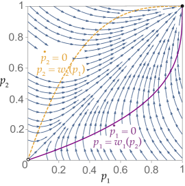
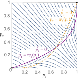
Figure 4.1: Illustrative Phase Plots ($\theta_{i}\equiv 3=u_{1}$; $u_{2}$ is either 3 or $\frac{1}{3}$ )

The figure illustrates the phase plots of sampling dynamics for two environments: (1) $\forall i\,\,\theta_{i}\equiv 3=u_{i}$ (left panel, a symmetric coordination game), and (2) $\forall i\,\,\theta_{i}\equiv 3=u_{1}=\frac{1}{u_{2}}$ (right panel, an antisymmetric coordination game). The solid purple (resp., dashed orange ) curve of $w_{1}\left(p_{2}\right)$ (resp., $w_{2}\left(p_{1}\right)$) shows the states for which $\dot{p}_{1}=0$ (resp., $\dot{p}_{2}=0$ ). The intersection points of these curves are the stationary states. A solid (resp., hollow) dot represents an asymptotically stable (resp., unstable) stationary state.

The following fact is immediate given the basic properties of binomial random variables.

Fact 1.

$w_{i}(p_{j})$ is a strictly increasing polynomial function that satisfies $w_{i}(0)=0$ and $w_{i}(1)=1$. This implies that the inverse function $w_{i}^{-1}:[0,1]\rightarrow[0,1]$ exists, is continuously differentiable, and that $w_{i}^{-1}(0)=0$ and $w_{i}^{-1}(1)=1.$

Fact 1 implies that the two curves intersect at $(0,0)$ and $(1,1)$.

Appendix A.4 presents the standard definitions of stationary states, asymptotically stable states, and unstable states. Observe that a state is stationary (i.e., it is a fixed point of the dynamics) iff it is an intersection point of the two curves $w_{1}$ and $w_{2}$.

Fact 2.

State $\boldsymbol{p}$ is stationary $\iff$ $p_{2}=w_{2}\left(p_{1}\right)$ and $p_{1}=w_{1}\left(p_{2}\right)$ $\implies$ $p_{1}=w_{1}(w_{2}(p_{1}))$ and $p_{2}=w_{2}(w_{1}(p_{2})).$

4.2 Asymptotic Stability of Pure Equilibria

To state our next results, it will be helpful to consider the condition in which a single appearance of a rare action can change the behavior of a new agent. Specifically, consider a new agent in population $i$ with a sample size of $k$. Observe that:

1. Action $a_{i}$ induces a weakly higher payoff against a sample with an opponent’s action $a_{j}$ (and $k-1$ opponents’ actions $b_{j})$ iff $u_{i}\geq k-1\Leftrightarrow k\leq u_{i}+1$.

2. Action $b_{i}$ induces a strictly higher payoff against a sample with an opponent’s action $b_{j}$ (and $k-1$ opponents’ actions $a_{j})$ iff $1>\left(k-1\right)u_{i}\Leftrightarrow k<\frac{1}{u_{i}}+1$.

Next we define $m$-bounded expectation as the expected value of a probability distribution when taking into account only values smaller than $m$. Formally:

Definition 2.

The $m$-bounded expectation $\mathbb{E}_{\leq m}$ (resp., $\mathbb{E}_{<m}$) of distribution $\theta_{i}$ with support on integers is $\mathbb{E}_{\leq m}\left(\theta_{i}\right)=\sum_{1\leq k\leq m}\theta_{i}\left(k\right)\cdot k$ (resp., $\mathbb{E}_{<m}\left(\theta_{i}\right)=\sum_{1\leq k<m}\theta_{i}\left(k\right)\cdot k$).

Proposition 1 characterizes the asymptotic stability of the pure equilibria. It shows that asymptotic stability depends only on whether the product of the bounded expectations of the distributions of sample sizes is larger or smaller than one, where the bound of each distribution is the maximal sample size for which a single appearance of a rare action can change the behavior of a new agent. Formally:

Proposition 1.

1. $\mathbb{E}_{<\frac{1}{u_{1}}+1}\left(\theta_{1}\right)\cdot\mathbb{E}_{<\frac{1}{u_{2}}+1}\left(\theta_{2}\right)=\theta_{1}\left(1\right)\cdot\mathbb{E}_{<\frac{1}{u_{2}}+1}\left(\theta_{2}\right)>1\,\Rightarrow$ a=$\left(a_{1},a_{2}\right)$ is unstable;

2. $\mathbb{E}_{<\frac{1}{u_{1}}+1}\left(\theta_{1}\right)\cdot\mathbb{E}_{<\frac{1}{u_{2}}+1}\left(\theta_{2}\right)=\theta_{1}\left(1\right)\cdot\mathbb{E}_{<\frac{1}{u_{2}}+1}\left(\theta_{2}\right)<1\,\Rightarrow$ $\boldsymbol{a}$ is asymptotically stable;

3. $\mathbb{E}_{\leq u_{1}+1}\left(\theta_{1}\right)\cdot\mathbb{E}_{\leq u_{2}+1}\left(\theta_{2}\right)>1\,\Rightarrow$ b=$\left(b_{1},b_{2}\right)$ is unstable; and

4. $\mathbb{E}_{\leq u_{1}+1}\left(\theta_{1}\right)\cdot\mathbb{E}_{\leq u_{2}+1}\left(\theta_{2}\right)<1\,\Rightarrow$ b=$\left(b_{1},b_{2}\right)$ is asymptotically stable.

Sketch of Proof.

Consider a slightly perturbed state $(1-\epsilon_{1},1-\epsilon_{2})$ near $\boldsymbol{a}=\left(1,1\right)$ (the argument for $\boldsymbol{b}$ is analogous) in which almost all agents play action $a_{i}$. The event of two rare actions ($b_{i}$-s) appearing in a sample of a new agent has a negligible probability of $O(\epsilon_{i}^{2})$. If a new agent has a sample size of $k$, then the probability of a rare action appearing in the sample is approximately $k\cdot\epsilon_{j}.$ This rare appearance changes the perceived best response of a new agent in population $i$ iff $k$ is smaller than $\frac{1}{u_{i}}+1$. Thus, the probability that a new agent in population $i$ adopts the rare action $b_{i}$ is equal to $\mathbb{E}_{<\frac{1}{u_{i}}+1}\left(\theta_{i}\right)$. This implies that the product of the share of new agents adopting a rare action in each population is $\epsilon_{1}\cdot\mathbb{E}_{<\frac{1}{u_{1}}+1}\left(\theta_{1}\right)\cdot\epsilon_{2}\cdot\mathbb{E}_{<\frac{1}{u_{1}}+1}\left(\theta_{2}\right)$. This shows that the share of agents playing rare actions gradually increases (resp., decreases) if $\mathbb{E}_{<\frac{1}{u_{1}}+1}\left(\theta_{1}\right)\cdot\mathbb{E}_{<\frac{1}{u_{1}}+1}\left(\theta_{2}\right)>1$ (resp., $\mathbb{E}_{<\frac{1}{u_{1}}+1}\left(\theta_{1}\right)\cdot\mathbb{E}_{<\frac{1}{u_{1}}+1}\left(\theta_{2}\right)<1),$ which implies instability (resp., asymptotic stability). Finally, observe that our assumption that $u_{1}\geq 1$ implies that $\frac{1}{u_{1}}+1\leq 2$, which, in turn, implies that $\theta_{1}\left(1\right)=\mathbb{E}_{<\frac{1}{u_{1}}+1}\left(\theta_{1}\right)$. See Appendix A.5 for a formal proof. ∎

An interesting implication of Proposition 1 is the substantial difference in the stability of a $\frac{1}{2}$-dominant equilibrium and a risk-dominated equilibrium (related results for symmetric coordination games are derived in Oyama, Sandholm, and Tercieux, 2015). A risk-dominated equilibrium (say, $\boldsymbol{b}$) is unstable as long as sufficiently many agents have samples that are not too large (i.e., samples below $u_{i}+1$). The process inducing instability is as follows. A small perturbation of a few agents who play $\boldsymbol{a}_{i}$ induces a slightly larger number of new agents to observe $\boldsymbol{a}_{i}$ at least once in their samples, which induces them to play $a_{i}$ as well, which allows the small perturbations to gradually increase, until, at the end of the process, everyone plays the $\frac{1}{2}$-dominant action $\boldsymbol{a}_{i}$.

By contrast, any $\frac{1}{2}$-dominant equilibrium is asymptotically stable. To see this, observe that if $\boldsymbol{a}$ is a weakly $\frac{1}{2}$-dominant equilibrium (i.e., if $u_{2}\geq 1$, where the weak inequality is due to the tie-breaking rule in favor of $a_{i}$) then $\frac{1}{u_{2}}+1\leq 2$, which implies that $\mathbb{E}_{<\frac{1}{u_{2}}+1}\left(\theta_{2}\right)=\theta_{2}\left(1\right)<1$. This implies that $\mathbb{E}_{<\frac{1}{u_{1}}+1}\left(\theta_{1}\right)\cdot\mathbb{E}_{<\frac{1}{u_{2}}+1}\left(\theta_{2}\right)=\theta_{1}\left(1\right)\cdot\theta_{2}\left(1\right)<1$, and thus $\boldsymbol{a}$ is asymptotically stable. This implies that:

Corollary 1.

Any $\frac{1}{2}$-dominant equilibrium is asymptotically stable.

Thus, only in games in which neither equilibrium is $\frac{1}{2}$-dominant (i.e., those in which $u_{2}<1\leq u_{1}$), might it be possible for both pure equilibria to be unstable.

4.3 Global Convergence Results

The following definition of neighboring stationary states will be helpful for stating our results.

Definition 3.

Two stationary states $\underline{\boldsymbol{p}},\boldsymbol{\overline{p}}$ are said to be neighbors if there does not exist any stationary state $\hat{\boldsymbol{p}}$ such that $\underline{p}_{i}<\hat{p}_{i}<\overline{p}_{i}$.

We first show that the populations always converge to a stationary state.

Proposition 2.

$\lim_{t\rightarrow\infty}\mathbf{p}\left(t\right)$ converges to a stationary state for any $\textbf{p}(0).$

Proof.

Since the function $w_{i}(\cdot)$ is a polynomial of degree $\max(\textrm{supp}\left(\theta_{i}\right))>1,$ it follows that $w_{i}\left(w_{j}\left(\cdot\right)\right)$ is a polynomial of a finite degree strictly larger than 1. As the stationary states are characterized by the intersection of the curves $p_{1}=w_{1}(p_{2})$ and $p_{2}=w_{2}(p_{1}),$ we can conclude that there are a finite number of stationary states. The result now follows from the following claims whose proofs are presented in Appendix A.6.

Claim 1 (Any trajectory reaches the area between the curves).

Either $\lim_{t\rightarrow\infty}\mathbf{p}\left(t\right)$ converges to a stationary state, or there exists $t<\infty$ such that either $w_{1}^{-1}\left(p_{1}\left(t\right)\right)\leq p_{2}\left(t\right)\leq w_{2}\left(p_{1}\left(t\right)\right)$ or $w_{2}\left(p_{1}\left(t\right)\right)\leq p_{2}\left(t\right)\leq w_{1}^{-1}\left(p_{1}\left(t\right)\right)$.

The intuition for Claim 1 (see Figure 4.1) is that populations starting at an initial state below (resp., above) the two curves move upward and to the left (resp., downward and to the right) until reaching the area between the two curves.

Claim 2 (Convergence from the area between the curves to a neighboring stationary state).

Let $\boldsymbol{p}\left(t\right)$ be an interior state for some $t\geq 0$ and let $\underline{\boldsymbol{p}},\boldsymbol{\overline{p}}$ be neighboring stationary states with $\underline{p}_{i}\leq p_{i}(t)\leq\overline{p}_{i}$. We have,

1. If $p_{2}\left(t\right)\in\left[w_{1}^{-1}\left(p_{1}\left(t\right)\right),w_{2}\left(p_{1}\left(t\right)\right)\right]$, then $\lim_{t\rightarrow\infty}\mathbf{p}\left(t\right)=\overline{\boldsymbol{p}}$, and

2. If $p_{2}\left(t\right)\in\left[w_{2}\left(p_{1}\left(t\right)\right),w_{1}^{-1}\left(p_{1}\left(t\right)\right)\right]$, then $\lim_{t\rightarrow\infty}\mathbf{p}\left(t\right)=\underline{\boldsymbol{p}}$.∎

The intuition for Claim 2 (see Figure 4.1) is that in the area between the two curves in the interval between $\underline{\boldsymbol{p}}$ and $\boldsymbol{\overline{p}}$, the populations either always move upward and to the right (in which case they must converge to $\boldsymbol{\overline{p}}$), or they always move downward and to the left (in which case they must converge to $\boldsymbol{\underline{p}}$).

Next we show that if any initial interior state converges to one of the pure equilibria, then this equilibrium is asymptotically stable (as defined in Appendix A.4).

Lemma 1.

Assume that $\textbf{p}(0)\neq(0,0)$ and $\lim_{t\rightarrow\infty}\mathbf{p}\left(t\right)=(0,0)$; then $(0,0)$ is asymptotically stable. The same result holds when $(1,1)$ replaces $(0,0).$

Proof.

See Appendix A.7. ∎

We now show that the populations converge from almost any initial state to an interior stationary state if (and essentially only if) the product of the bounded expectation of the distribution of sample sizes in each population and the share of agents with sample size 1 in the other population is larger than 1.

Theorem 1.

Assume that $u_{2}<1\leq u_{1}$ (no $\frac{1}{2}$-dominant equilibrium). Then

1. Global convergence to miscoordination: Assume that

   $$\theta_{1}\left(1\right)\cdot\mathbb{E}_{<\frac{1}{u_{2}}+1}\left(\theta_{2}\right)>1\,\,\textrm{\,\,and}\,\,\,\,\theta_{2}\left(1\right)\cdot\mathbb{E}_{\leq u_{1}+1}\left(\theta_{2}\right)>1.$$

   If $\boldsymbol{p}(0)\notin\left\{(0,0),(1,1)\right\}$, then $\lim_{t\rightarrow\infty}\mathbf{p}\left(t\right)\notin\left\{(0,0),(1,1)\right\}$.

2. Local convergence to coordination: Assume that

   $$\theta_{1}\left(1\right)\cdot\mathbb{E}_{<\frac{1}{u_{2}}+1}\left(\theta_{2}\right)<1\,\,\,\,\textrm{or}\,\,\,\,\theta_{2}\left(1\right)\cdot\mathbb{E}_{\leq u_{1}+1}\left(\theta_{2}\right)<1.$$

   Then at least one of the pure equilibria is asymptotically stable.

Proof.

1. Proposition 1 implies that both pure stationary states are unstable. Proposition 2 and Lemma 1 imply that from almost any initial state, the population converges to an interior stationary state.

2. Proposition 1 implies that at least one of the pure equilibria is asymptotically stable, which implies that some interior initial states converge to a pure equilibrium. ∎

Theorem 1 shows that global convergence to miscoordination requires heterogeneity in the sample sizes in each population that includes both agents with a small sample size of one, and agents with larger samples (but not too large, as they must be below the bound for which a single observation of a rare action can influence behavior). Specifically, in each population it is required that the product of (1) the share of agents with a sample size of 1 and (2) the bounded expected sample size should be sufficiently large.

Observe that the farther the $u_{i}$-s are from 1, the higher (i.e., less restrictive) the bounded expected value is. That is, games in which for each population one of the actions is much riskier than the other action (i.e., for population 2, action $a_{2}$ is much riskier than action $a_{1},$ while for population 1, action $a_{1}$ is much riskier than action $a_{2}$) are more likely have stable miscoordination.

The following example demonstrates global convergence to miscoordination, and the fact that the stability of pure states is nonmonotone in the sample sizes.

Example 1 (Nonmonotone Impact of Sample Size).

Consider a battle of the sexes game in which $u_{1}=5$ and $u_{2}=0.2$ and both populations have the same distribution of sample sizes. Consider 3 distributions of sample sizes, in each of which half of the players in the population have sample size 1. In the first distribution (left panel of Figure 4.2) the remaining half of the players have sample size 3, in the second distribution (middle panel) they have sample size 5, and in the third distribution (right panel of Figure 4.2) they have sample size 7. Observe that the second distribution satisfies the condition for global convergence to miscoordination, i.e.,

$$\theta_{1}\left(1\right)\cdot\mathbb{E}_{<\frac{1}{u_{2}}+1}\left(\theta_{2}\right)=\theta_{1}\left(1\right)\cdot\mathbb{E}_{<6}\left(\theta_{2}\right)=\theta_{1}\left(1\right)\cdot\mathbb{E}\left(\theta_{2}\right)=0.5\cdot 3>1$$

(and the same holds for population 2). Indeed, the middle phase plot shows that the populations converge from any interior state to the state $\left(0.37,0.63\right)$ with substantial miscoordination (specifically, the agents miscoordinate and get a payoff of zero in 46%$\approx 2\cdot 0.37\cdot 0.63$ of the interactions). By contrast, either decreasing the larger sample size from 5 to 2, or increasing it to 7, yields a product $\theta_{1}\left(1\right)\cdot\mathbb{E}_{<\frac{1}{u_{2}}+1}\left(\theta_{2}\right)$ that is strictly smaller than 1 ($\theta_{1}\left(1\right)\cdot\mathbb{E}\left(\theta_{2}\right)=0.5\cdot 1.5<1$ in the first case, and $\theta_{1}\left(1\right)\cdot\mathbb{E}_{<6}\left(\theta_{2}\right)=\theta_{1}\left(1\right)\cdot\theta_{1}\left(1\right)=0.5\cdot 0.5<1$ in the second case). The left and right panels of Figure 4.2 illustrate that in both cases almost all initial states converge to a pure state. Thus, changing sample sizes of agents has a nonmonotone impact on the stability of miscoordination.

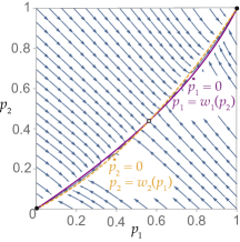
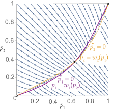
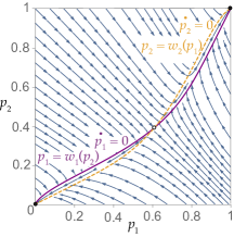
Figure 4.2: Illustration of Theorem 1 and Example 1

The figure illustrates the phase plots for three environments. In each environment, the underlying coordination game is antisymmetric with $u_{1}=5$ and $u_{2}=0.2$, and 50% of the agents in each population have sample size 1. In the environment illustrated in the left (resp., middle, right) panel the remaining half of the players in the population have sample size 2 (resp., 5, 7). The middle panel shows global convergence to the interior state with miscoordination $\left(0.37,.0.63\right)$, while the other two panels show global convergence to one of the pure equilibria.

5 Homogeneity and Unstable Miscoordination

In this section, we show that heterogeneity is necessary for stable miscoordination. Specifically, we show that any environment in which all agents in each population have the same sample size admits at most one interior stationary state, and that this state is unstable.

Auxiliary Results

We begin by showing that a stationary state $\hat{\boldsymbol{p}}$ is asymptotically stable iff the curve $w_{2}$ is above the curve $w_{1}^{-1}$ in a left neighborhood of $\hat{\boldsymbol{p}}$, and it is below the curve $w_{1}^{-1}$ in a right neighborhood of $\hat{\boldsymbol{p}}$.

Lemma 2.

Let $\hat{\boldsymbol{p}}$ be a stationary state. $\hat{\boldsymbol{p}}$ is asymptotically stable if both of the following conditions hold:

1. Left neighborhood: If $\hat{p}_{1}>0$ then there exists $\underline{p}_{1}\in\left(0,\hat{p}_{1}\right)$ such that $w_{2}\left(p_{1}\right)>w_{1}^{-1}\left(p_{1}\right)$ for any $p_{1}\in\left(\underline{p}_{1},\hat{p}_{1}\right)$, and

2. Right neighborhood: If $\hat{p}_{1}<1,$ then there exists $\overline{p}_{1}\in\left(\hat{p}_{1},1\right)$ such that $w_{2}\left(p_{1}\right)<w_{1}^{-1}\left(p_{1}\right)$ for any $p_{1}\in\left(\hat{p}_{1},\overline{p}_{1}\right)$.

Moreover, if either of the above two conditions is not satisfied, then $\hat{\boldsymbol{p}}$ is unstable.

Proof.

See Appendix A.8. ∎

Lemma 2 implies that the neighbor of an asymptotically stable state must be unstable.

Corollary 2.

Let $\underline{\boldsymbol{p}}\neq\overline{\boldsymbol{p}}$ be two neighboring stationary states. If $\underline{\boldsymbol{p}}$ is asymptotically stable, then $\overline{\boldsymbol{p}}$ is unstable.

Proof.

Without loss of generality assume that $\underline{p}_{1}<\overline{p}_{1}$. Due to Claim 2, the fact that $\underline{\boldsymbol{p}}$ is asymptotically stable implies that $w_{2}\left(p_{1}\right)>w_{1}^{-1}\left(p_{1}\right)$ for any $p_{1}\in\left(\underline{p}_{1},\overline{p}_{1}\right)$ which, in turn implies that $\overline{\boldsymbol{p}}$ is unstable.∎

A Property of Binomial Distributions

The main result is implied by a property of binomial distributions (which may be of independent interest). Recall our notation of $X(k,p)\sim Bin\left(k,p\right)$ denoting a random variable with a binomial distribution. Define $F_{m}^{k}\left(p\right)\equiv\Pr\left(X\left(k,p\right)\geq m\right)$ as the probability of having at least $m$ successes in $k$ trials when the probability of success in each trial is $p$. Observe that $F_{m}^{k}\left(0\right)=0$, $F_{m}^{k}\left(1\right)=1,$ and $\left(F_{m}^{k}\right)^{\prime}>0$. It is known that $F_{m}^{k}$ has at most one interior fixed point, i.e.,

Fact 3 (Green, 1983, Theorem 1).

Fix arbitrary integers $0<m\leq k$. Then there is at most one $p\in\left(0,1\right)$ such that $F_{m}^{k}\left(p\right)=p.$

We extend it by showing that the same is true also for a composition of any two cumulative binomial distributions, i.e., that $F_{m_{1}}^{k_{1}}\circ F_{m_{2}}^{k_{2}}$ has at most one interior fixed point.

Proposition 3.

Fix arbitrary integers satisfying $0<m_{1}\leq k_{1}$ and $0<m_{2}\leq k_{2}$. There exists at most one $p\in\left(0,1\right)$ such that $\left(F_{m_{1}}^{k_{1}}\circ F_{m_{2}}^{k_{2}}\right)\left(p\right)=p$.

The proof, which is detailed in Appendix A.3, shows that $F_{m_{1}}^{k_{1}}\circ F_{m_{2}}^{k_{2}}$ has at most one inflection point, which implies that there exists at most one interior fixed point.

Main Result

We now present the main result of this section: any environment with homogeneous sample sizes admits at most one interior stationary state that is unstable. This implies that almost all initial states converge to one of the pure equilibria.

Theorem 2.

Assume that $\theta_{i}\equiv k_{i}>1$ for each $i\in\left\{1,2\right\}$. There exists at most one interior stationary state, and this state (if it exists) is unstable.

Proof.

The fact that $\theta_{i}\equiv k_{i}>1$ implies that $w_{i}\left(p\right)=F_{m_{i}}^{k_{i}}\left(p\right)$ for some $1\leq m_{i}\leq k_{i}$. This implies that any stationary state $\boldsymbol{p}^{\ast}$ must satisfy $\left(F_{m_{1}}^{k_{1}}\circ F_{m_{2}}^{k_{2}}\right)\left(p_{1}^{\ast}\right)=p_{1}^{\ast}$. Proposition 3 implies that this holds for at most one interior state $\hat{\boldsymbol{p}}$. Therefore, the stationary state $\hat{\boldsymbol{p}}$ (if it exists) is a neighbor of both pure stationary states $\left(0,0\right)$ and $\left(1,1\right)$. Proposition 1 and the fact that no agents have sample size of 1 implies that at least one of these pure states is asymptotically stable. Finally, Corollary 2 implies that $\hat{\boldsymbol{p}}$ is unstable. ∎

6 Heterogeneity and Stable Miscoordination

The conditions presented for global convergence to miscoordination in Section 4 are somewhat narrow in the sense of requiring sufficiently many agents with sample size one. In this section we show that a much broader set of heterogeneous distributions of sample sizes can induce asymptotically stable states with miscoordination.

Specifically, we show that essentially any distribution of sample sizes that combines agents with small samples and agents with large samples induces locally stable miscoordination if the $u_{i}$-s are not too close to one. As demonstrated below, this type of heterogeneity in the sample sizes is plausible in various setups.

Example 2.

In housing markets (in which the bargaining situations can be modeled as hawk-dove coordination games), it is often the case that each population includes two types of agents: (1) professional real-estate investors, and (2) people who buy/sell houses only a couple of times during their life. It seems plausible that the real-estate investors have reliable information on the aggregate behavior (captured in our model by having large samples), while the remaining agents are likely to have limited, anecdotal evidence about the aggregate behavior (modeled by having small samples).

Result

Recall (Theorem 2) that all interior equilibria are unstable if all agents in each population have the same size. Our final result shows that, perhaps surprisingly, one can always add agents with large samples, and obtain an asymptotically stable interior equilibrium with miscoordination, provided that the $u_{i}$-s are not too close to one.

We formally define adding agents with large samples as follows. Given two sample sizes $k,\bar{k}$ and $\alpha\in(0,1)$, let $k\alpha\bar{k}$ be the distribution of sample sizes that assigns mass $\alpha$ to sample size $k$ and mass $1-\alpha$ to sample size $\bar{k}$.

Theorem 3.

Fix any pair of sample sizes $k_{1},k_{2}>1$. Then there exist $r,\alpha_{1},\alpha_{2}\in(0,1)$, such that for any $u_{1},u_{2}\notin(r,\frac{1}{r})$ the environment $\left(\boldsymbol{u},\left(k_{1}\alpha_{1}\bar{k},k_{2}\alpha_{2}\bar{k}\right)\right)$ admits an asymptotically stable interior state for any sufficiently large $\bar{k}$.

Proof idea (see Appendix A.9 for a formal proof).

We present one argument for games with a $\frac{1}{2}$-dominant equilibrium, and another for those without. The arguments are illustrated in the phase plots of Figure 6.1.

1. Games with a $\frac{1}{2}$-dominant equilibrium: Assume that $u_{i}>k_{i}$ for each $i$. Proposition 1 implies that the risk-dominated equilibrium $\boldsymbol{b}$ is unstable when all agents have sample size $k_{i}$. Observe that adding agents with large samples decreases the average probability of new agents playing $a_{i}$ in state $\left(\epsilon_{1},\epsilon_{2}\right)$ near $\boldsymbol{b}$. We choose $\alpha_{i}$, such that the share of new agents playing action $a_{i}$ (1) is above $\epsilon_{j}$ in state $\left(\epsilon_{1},\epsilon_{2}\right)$, and (2) is below $p_{j}$ in an interior state $\boldsymbol{\hat{p}}$ (this is possible because $\frac{w_{i}\left(p_{j}\right)}{p_{j}}$ is decreasing in small $p_{j}$-s). This, in turn, implies that there is a stable interior state between $\boldsymbol{b}$ and $\boldsymbol{\hat{p}}$.

2. Games without a $\frac{1}{2}$-dominant equilibrium: Observe that $w_{i}^{k_{i}}\left(p_{j}\right)$ remains the same for all values of $u_{i}$ that are sufficiently far from one ($u_{1}>k_{1}$, $u_{2}<\frac{1}{k_{2}}$), while the interior Nash equilibrium $p^{NE}_{1}$ (resp., $p^{NE}_{2}$) converges to 0 (resp., 1) as $u_{1}$ converges to infinity (resp., as $u_{2}$ converges to zero). Thus, for $u_{i}$-s sufficiently far from 1, $p_{2}^{NE}<\frac{w_{2}^{\theta_{2}}\left(\frac{1}{2}\right)}{2}$. We show that this implies that there must be an unstable stationary state with $p_{1}<\frac{1}{2}$ and $p_{2}\simeq p_{2}^{NE}<\frac{1}{2}$. By an analogous argument, there is an unstable stationary state with $p_{1}\simeq p_{1}^{NE}>\frac{1}{2}$ and $p_{2}>\frac{1}{2}$. This implies that there must be an asymptotically stable interior state between these two unstable states. ∎

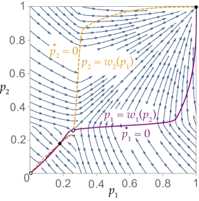
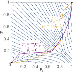
Figure 6.1: Illustrative Phase Plots for Theorem 3 (Locally Stable Miscoordination)

The left panel illustrates the symmetric game $u_{1}=u_{2}=2.5$, where 40% (resp., 60%) of the agents in each population have sample size 3 (resp., 1,000). The pure risk-dominated equilibrium $\left(0,0\right)$ is unstable, and its neighbor the interior stationary state with miscoordination $\left(0.18,0.18\right)$ is asymptotically stable. The right panel illustrates the antisymmetric game $u_{1}=\frac{1}{u_{2}}=5$, where 50% (resp., 50%) of the agents have sample size 2 (resp., 1,000). The mixed Nash equilibrium of this game is $\left(\frac{5}{6},\frac{1}{6}\right)$. The environment admits three interior stationary states: two unstable interior stationary states where one of the coordinates is close to the Nash equilibrium: $\left(0.6,0.18\right)$ and $\left(0.82,0.3\right)$, and a stable interior stationary state at $\left(0.73,0.27\right)$.

Remark 3.

For simplicity, Theorem 3 deals with a heterogeneous population that combines two sample sizes, $k_{i}$ and $\bar{k}.$ The proof’s argument can be adapted in a straightforward way to populations combining some agents who have arbitrary sample sizes (i.e., an arbitrary distribution $\theta_{i}$ replaces the arbitrary $k_{i}$), and some agents who have sufficiently large sample sizes (i.e., not necessarily all of the agents with large samples have the same sample size of $\bar{k}).$

Non-Payoff-Maximizing Behavior of Agents with Small Samples

Observe the interior stable state is (generically) not a mixed Nash equilibrium. For example, in the environment illustrated in the left panel of Figure 3 in which $u_{i}=2.5$, $\theta_{i}\left(3\right)=40\%$ and $\theta_{i}\left(1,000\right)=60\%$ for each population $i$, the interior stable state is $\left(0.17,0.17\right)$, while the mixed Nash equilibrium is $\left(0.28,0.28\right)$. This implies that one of the actions is the unique true best response to the opponent’s behavior (action $b_{i}$ in the example). This unique best response is played essentially by all agents with a large sample size of 1,000. By contrast, about $45\%$ of the agents with a small sample size of $3$ observe action $a_{-i}$ at least once in their sample, and play action $a_{i}$ due to an erroneous belief (based on their small sample) that the frequency of $a_{-i}$ is at least $\frac{1}{3}$. As a result, the average payoff to agents with a small sample is only 0.75, which is 8% smaller then the payoff of 0.82 to agents with a large sample.

This raises the question of why the agents with small samples do not learn to increase their samples, or why they are not driven out of the population. We suggest two explanations for this. The first is setups like our motivating example of a housing market that combine both inexperienced players (who have little experience in buying/selling houses) and experienced players (real-estate investors). In such setups, it seems likely that the inexperienced agents might have very limited (or costly) access to large samples (and a continuous inflow of inexperienced traders prevents them from being driven out of the market). Another reason why some players do not exert effort to increase their sample sizes is the “the law of small numbers,” which is the commonly believed bias that small samples well represent large populations (Tversky and Kahneman, 1971).

7 Comparison with Logit Dynamics

The main candidate in the existing literature to induce stable miscoordination in coordination games is logit dynamics. In this section we numerically demonstrate that (1) standard logit dynamics with a homogeneous level of noise in each population can induce stable miscoordination only with high levels of noise that seem implausible, and (2) a variant of logit dynamics with heterogeneity in the noise level can induce stable miscoordination with substantially lower levels of noise. This suggests that our key insight that stable miscoordination is induced by heterogeneous noise might hold in various classes of dynamics, and not only in sampling dynamics.

Standard (Homogeneous) Logit Dynamics

Logit dynamics (introduced in Fudenberg and Levine, 1995; see Sandholm, 2010, Section 6.2.3 for a textbook exposition) are characterized by a single parameter $\eta_{i}$ that describes the noise level for each population $i$. If player $i$ plays action $a_{i}$, she will get a payoff of $p_{j}\cdot u_{j}$. If she plays action $b_{i}$ she will get a payoff of $\left(1-p_{j}\right)\cdot 1$. Logit dynamics assume that the probability of revising agents playing action $a_{i}$ is proportional to $e^{\frac{\textrm{Payoff of $a_{i}$}}{\eta}}$. Specifically, logit dynamics are given by

$$w_{i}\left(p_{j}\right)\equiv w_{i}\left(\textbf{p}\right)=\frac{e^{\frac{p_{j}\cdot u_{j}}{\eta_{i}}}}{e^{\frac{1-p_{j}}{\eta_{i}}+}e^{\frac{p_{j}\cdot u_{j}}{\eta_{i}}}}.$$ (7.1)

Trivially, logit dynamics can induce substantial miscoordination by having high values of noise. The interesting question is whether stable miscoordination can be supported by a low level of noise. Our numerical analysis suggests that the answer is negative. In what follows we demonstrate that this is indeed the case. For example, when we revisit the the two examples of Figure 6.1 ($u_{1}=u_{2}=2.5$ and $u_{1}=\frac{1}{u_{2}}=5$), then the minimal level of noise that is required to sustain an asymptotically stable interior state in which each action is played with a probability of at least 10% is $\eta=1$ (see the left panel of Figure 7.1 for an illustration of the case of $u_{1}=u_{2}=2.5$). Such a high level of noise implies that 27% of the revising agents make the obvious mistake of playing $a_{i}$ when facing a population in which almost everyone plays $b_{j}$; by contrast, this obvious mistake is never made under action-sampling dynamics. Moreover, the average expected payoff obtained by revising agents who follow logit dynamics against an opponent population in which the share of agents playing action $a_{i}$ is distributed uniformly is 85% (resp., 71%) of the maximal payoff that can be obtained by payoff-maximizing agents in the first (resp., second) environment with $u_{1}=u_{2}=2.5$ (resp., $u_{1}=\frac{1}{u_{2}}=5$). By contrast, this average expected payoff is 98% (resp., 95%) of the maximal payoff under the sampling dynamics. Thus, stable cooperation can be supported by standard (homogeneous) logit dynamics only when the agents have high levels of noise.

Heterogeneous Logit Dynamics

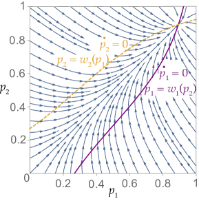
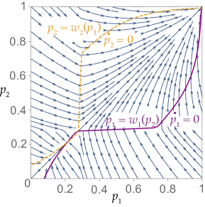
Figure 7.1: Supporting Stable Coordination with Heterogeneous Logit Dynamics

The figure revisits the symmetric game presented in the left panel of Figure 6.1 in which $u_{1}=u_{2}=2.5$. The left panel shows the phase plot of the minimal homogeneous level of noise, $\eta_{i}=1$, that sustains an asymptotically stable state in which each action is played with a probability of at least 10%. The right panel shows the phase plot of a heterogeneous variant of logit dynamics in which 55% of the the agents in each population have a moderate level of noise $\eta_{i}=0.55$ and 45% have a small level of noise $\eta_{i}=0.01$.

Next, consider a variant of logit dynamics in which there is heterogeneity in the level of noise for agents in each population. Specifically, in a population in which there are $n$ groups, the size of the $l$-th group is $\mu_{i}^{l}$ and its members have a noise level of $\eta_{i}^{l},$ the heterogeneous logit dynamics are given by

$$w_{i}\left(p_{j}\right)\equiv w_{i}\left(\textbf{p}\right)=\sum_{l}\mu_{i}^{l}\cdot\frac{e^{\frac{p_{j}\cdot u_{j}}{\eta_{i}^{l}}}}{e^{\frac{1-p_{j}}{\eta_{i}^{l}}+}e^{\frac{p_{j}\cdot u_{j}}{\eta_{i}^{l}}}}.$$ (7.2)

The numerical calculations demonstrate that heterogeneous noise levels can induce asymptotically stable miscoordination with relatively low levels of noise. Specifically, in both of the above examples ($u_{1}=u_{2}=2.5$, which is illustrated in the right panel of Figure 7.1, and $u_{1}=\frac{1}{u_{2}}=5$), populations in which 55% of the agents have a moderate level of noise (i.e., $\eta=0.55$) and 45% have a small level of noise (i.e., $\eta=0.01$) induce asymptotically stable states with miscoordination ($\left(0.21,0.21\right)$ in the right panel of Figure 7.1). Given these heterogeneous levels of noise, only 8% of the agents make the mistake of playing action $a_{i}$ when facing a population in which everyone plays $a_{j}$, and the average expected payoff obtained by playing against opponent populations in which the share of agents playing action $a_{i}$ is distributed uniformly is 96% (resp., 89%) of the maximal payoff that can be obtained by payoff-maximizing revising agents in the environment with $u_{1}=u_{2}=2.5$ (resp., $u_{1}=\frac{1}{u_{2}}=5$).

8 Conclusion

The conventional wisdom, which is supported by key results in evolutionary game theory, is that only pure (coordinated) outcomes are reasonable long-run predictions of behavior in coordination games. By contrast, we show that plausible learning dynamics, in which new agents rely on samples to estimate and best respond to the behavior of the opponents’ population, can induce stable miscoordination. This happens if there is heterogeneity in the sample sizes: some agents have accurate information based on large samples of the opponents’ aggregate behavior, while other agents rely on anecdotal evidence induced by small samples. We further show that stable miscoordination holds under a broad set of heterogeneous distributions of sample sizes, if for each player one of the actions in the underlying game is $q$-dominant for a sufficiently small $q$.

Although our analytical results focus on the specific family of sampling dynamics, the numerical results for logit dynamics suggest that qualitatively similar results are likely to hold under other learning dynamics, i.e., heterogeneous noise levels can induce stable miscoordination. Such heterogeneity is plausible in many applications, such as bargaining in housing markets, where some participants are professional investors, while other participants are inexperienced. The predictions of our model can be experimentally tested, as outlined Section 2.

Appendix A Appendix

A.1 Standard Representation of General Coordination Games

In this subsection we explain why the two-parameter standard representation (Table 2) captures w.l.o.g. any two-action coordination game (in line with Harsanyi and Selten’s () Axiom 2 of best-reply invariance).

The most general definition of a two-action coordination game is a game that admits two strict Nash equilibria. By relabeling the actions of player 1, we can assume w.l.o.g. that these two pure equilibria are $\left(a_{1},a_{2}\right)$ and $\left(b_{1},b_{2}\right)$ (i.e., if the two pure equilibria are $\left(a_{1},b_{2}\right)$ and $\left(b_{1},a_{2}\right)$, then we switch the labels of player 1’s actions: $a_{1}$$\leftrightarrow$$b_{1}).$ This implies that the left panel of Table 3 shows a parametric representation of all coordination games.

Table 3: Normalization of General Two-Action Coordination Games

Original Representation				Standard Representation
	$a_{2}$	$b_{2}$	$\begin{array}[]{c}\\ \\ \Rightarrow\\ \\ \\ \end{array}$		$a_{2}$	$b_{2}$
$~{}~{}a_{1}~{}~{}$	$\,\,{}_{\underset{\,}{{\color[rgb]{0,0,1}u_{11}}}}{\,{}^{\overset{\,}{v_{11}}}}$	$\,\,{}_{\underset{\,}{{\color[rgb]{0,0,1}u_{12}}}}{\,{}^{\overset{\,}{v_{12}}}}$		$~{}~{}a_{1}~{}~{}$	${}_{\frac{{\color[rgb]{0,0,1}u_{11}}-{\color[rgb]{0,0,1}u_{21}}}{{\color[rgb]{0,0,1}u_{22}-}{\color[rgb]{0,0,1}u_{1\underset{\,}{2}}}}}{\,{}^{\overset{}{\frac{v_{11}-v_{12}}{v_{22}-v_{21}}}}}$	$\,\,\,\,{}_{\underset{\,}{{\color[rgb]{0,0,1}0}}}{\,\,\,\,{}^{\overset{\,}{0}}}$
$~{}~{}b_{1}~{}~{}~{}$	$\,\,{}_{\underset{\,}{{\color[rgb]{0,0,1}u_{21}}}}{\,{}^{\overset{\,}{v_{21}}}}$	$\,\,{}_{\underset{\,}{{\color[rgb]{0,0,1}u_{22}}}}{\,{}^{\overset{\,}{v_{22}}}}$		$~{}~{}b_{1}~{}~{}~{}$	$\,\,{}_{\underset{\,}{{\color[rgb]{0,0,1}0}}}{\,\,\,\,\,\,\,\,\,{}^{\overset{\,}{0}}}$	$\,\,{}_{\underset{\,}{{\color[rgb]{0,0,1}1}}}\,\,\,{\,{}^{\overset{\,}{1}}}$
$\underset{}{{\color[rgb]{0,0,1}u_{11}>u_{21}},u_{22}>u_{12}}$, $\underset{}{v_{11}>v_{12}},\underset{}{v_{22}>v_{21}}$

Sampling dynamics (as defined in 3.1 and A.1) depend only on the differences between the payoffs a player can get by playing different actions (the same property holds for best-response dynamics and logit dynamics, which implies that the sets of Nash equilibria, quantal response equilibria, and evolutionary stable strategies depend only on these differences). These differences are invariant to subtracting a constant from all the payoffs of a player while fixing the opponent’s action (e.g., subtracting $u_{21}$ from all of Player 1’s first-column payoffs). Moreover, sampling dynamics (as well as all the other dynamics and solution concepts mentioned above) are invariant to dividing all of a player’s payoff by a positive constant (which preserves the vN–M utility). The left matrix in Table 3 is reduced to the right matrix by the following steps (none of which affect the sampling dynamics):

1. Three changes to Player 1’s payoffs: (I) subtracting $u_{21}$ from Player 1’s payoffs in her first column, (II) subtracting $u_{12}$ from Player 1’s payoffs in her second column, and (III) dividing Player 1’s payoff by ${\color[rgb]{0,0,1}u_{22}-}u_{12}$; and

2. Three changes to Player 2’s payoffs: (I) subtracting $v_{12}$ from Player 1’s payoffs in her first row, (II) subtracting ${\color[rgb]{180,00,00}v_{21}}$ from Player 1’s payoffs in her first row, and (III) dividing Player 1’s payoff by ${\color[rgb]{180,00,00}v_{22}-v_{21}}$.

Observe that the assumption that ${\color[rgb]{0,0,1}u_{1}}=\frac{{\color[rgb]{0,0,1}u_{11}}-{\color[rgb]{0,0,1}u_{21}}}{{\color[rgb]{0,0,1}u_{22}-}{\color[rgb]{0,0,1}u_{12}}}\geq 1$ in the standard representation of Table 2 is w.l.o.g.. If $\frac{{\color[rgb]{0,0,1}u_{11}}-{\color[rgb]{0,0,1}u_{21}}}{{\color[rgb]{0,0,1}u_{22}-}{\color[rgb]{0,0,1}{\color[rgb]{0,0,1}u_{12}}}}<1$, then we can multiply all of Player 1’s payoffs by $\frac{{\color[rgb]{0,0,1}u_{22}-}{\color[rgb]{0,0,1}{\color[rgb]{0,0,1}u_{12}}}}{{\color[rgb]{0,0,1}u_{11}}-{\color[rgb]{0,0,1}u_{21}}}$ and all of Player 2’s payoffs by ${\color[rgb]{180,00,00}\frac{v_{22}-v_{21}}{v_{11}-v_{12}}}$, relabel the actions $a_{i}\leftrightarrow b_{i}$ for both players, and obtain a standard representation as in Table 2 in which $u_{1}\geq 1$.

Example 3 (Hawk-Dove Games).

Consider a hawk-dove (aka, chicken) game, which can be interpreted as a game of bargaining over the price of an asset (e.g., a house) between a buyer and a seller. Each player can either insist on a more favorable price (“hawk”) or agree to a less favorable price in order to close the deal (“dove”). The left panel of Table 4 shows the payoffs of a hawk-dove game. Two doves agree on an equally favorable price (which gives both players a relatively high payoff normalized to one). A hawk obtains a favorable price when matched with a dove (which increases the payoff to the hawk by $g\in(0,1)$, while reducing the dove’s payoff by $l\in(0,1)$), but faces a high probability of bargaining failure when matched with another hawk (which would yield a low payoff of zero to both hawks).

Observe that a hawk-dove game can be transformed to our standard representation of a coordination game (the right panel of Table 4) as follows: (1) relabel the actions of player 1 such that $a_{1}=d_{1}$ and $b_{1}=h_{1}$ (while keeping the actions of Player 2 as $a_{2}=h_{2}$ and $b_{2}=d_{2}$), (2) subtract a payoff of 1 from Player 1’s payoffs in her second column and from Player 2’s payoffs in her first column, and (3) divide all the payoffs of Player 1 by $g$, and all payoffs of Player 2 by $1-l$. Observe that the induced standard representation is antisymmetric, i.e., $u_{1}=\frac{{\color[rgb]{0,0,1}1-l}}{g}=\frac{1}{u_{2}}$.

Table 4: Normalization of Hawk-Dove Games ($g,l\in\left(0,1\right)$)

Original Representation				Standard Representation
	$h_{2}$	$d_{2}$	$\begin{array}[]{c}\\ \\ \Rightarrow\\ \\ \\ \end{array}$		$a_{2}=h_{2}$	$b_{2}=d_{2}$
$~{}h_{1}$	$\,\,{}_{\underset{\,}{{\color[rgb]{0,0,1}0}}}{\,{}^{\overset{\,}{0}}}$	${}_{\underset{\,}{{\color[rgb]{0,0,1}1+g}}}\,\,\,{\,{}^{\overset{\,}{1-l}}}$		$~{}~{}~{}a_{1}=d_{1}~{}$	$\,\,{}_{\underset{\,}{{\color[rgb]{0,0,1}\frac{{\color[rgb]{0,0,1}1-l}}{g}}}}\,\,\,{\,{}^{\overset{\,}{\frac{g}{1-l}}}}$	$\,{}_{\underset{\,}{{\color[rgb]{0,0,1}0}}}{\,{}^{\overset{\,}{0}}}$
$~{}d_{1}$	$\,\,{}_{\underset{\,}{{\color[rgb]{0,0,1}1-l}}}\,\,\,{\,{}^{\overset{\,}{1+g}}}$	${}_{\underset{\,}{{\color[rgb]{0,0,1}1}}}\,\,\,{\,{}^{\overset{\,}{1}}}$		$~{}~{}~{}b_{1}=h_{1}~{}~{}$	$\,\,{}_{\underset{\,}{{\color[rgb]{0,0,1}0}}}{\,\,\,\,\,\,\,{}^{\overset{\,}{0}}}$	$\,\,{}_{\underset{\,}{{\color[rgb]{0,0,1}1}}}{\,{}^{\overset{\,}{1}}}$

A.2 One-Population Dynamics

In the main text, we derived results for general coordination games under two-population dynamics. In this appendix, we show that analogous results hold for symmetric coordination games under one-population dynamics.

Adapted Definitions

An environment $((u_{1},u_{2}),(\theta_{1},\theta_{2}))$ is symmetric if $u_{1}=u_{2}$ and $\theta_{1}=\theta_{2}$. As we focus on symmetric environments here, we omit the subscript $i$ referring to the population from the parameters $u_{i},\theta_{i}$, the actions $a_{i},b_{i}$, and the sampling dynamics $w_{i}.$ Thus, a symmetric environment is denoted by $(u,\theta)$, where $u$ is the payoff to each player when coordinating on $a$, and $\theta$ is the distribution of sample size of each player.

Under one-population dynamics, the state is denoted by a single number $p\in(0,1)$ that describes the share of players who play action $a$ in the population. At each time $t,$ a constant flow (normalized to one) of agents die, and are replaced by new agents. The sample sizes of the new agents are distributed according to $\theta$. Each $k$-agent (a new agent with sample size $k$) randomly and independently samples $k$ players and observes the actions that they played. Thus, the one-dimensional sampling dynamics is given by $\dot{p}=w(p)-p$, where

$$w\left(p\right)=\sum_{k\in\text{supp}\left(\theta\right)}\theta(k)\cdot\Pr\left(X\left(k,p\right)\geq\frac{k}{u+1}\right).$$ (A.1)

In the above equation, $X(k,p)$ denotes a binomial random variable with parameters $k$ and $p.$ Analogous arguments to those presented in Appendix A.1 imply that any symmetric coordination game can be normalized w.l.o.g. to the standard form with a single parameter $u$.

Adaptation of Results

We next show that in symmetric coordination games, the set of stationary states and the set of asymptotically stable stationary states coincide under the one-population dynamics and the two-population dynamics. This implies that all our main-text results hold also for one-population dynamics in symmetric coordination games.

We first show that the sets of stationary states coincide in both sets of dynamics.

Proposition 4.

Let $(u,\theta)$ be a symmetric environment. State $(p_{1},p_{2})$ is stationary under two-population dynamics iff the state is symmetric (i.e., $p\equiv p_{1}=p_{2}$), and $p$ is stationary under one-population dynamics.

Proof.

Assume that $(p_{1},p_{2})$ is a stationary state under two-population dynamics. Assume to the contrary that $p_{1}\neq p_{2}$. w.l.o.g., assume that $p_{1}<p_{2}$. The fact that $w$ is strictly increasing implies that $p_{2}=w(p_{1})<w(p_{2})=p_{1}$, and we get a contradiction. Thus, we know that all stationary states under two-population dynamics are symmetric (i.e., of the form $(p,p)$ in symmetric environments). Observe that a symmetric state $(p,p)$ is stationary under two-population dynamics iff $p$ is stationary under one-population dynamics, because stationarity under both dynamics is characterized by the equation $p=w(p)$. ∎

The fact that one-population dynamics are one-dimensional implies the following simple and well-known fact:

Fact 4.

Stationary state $p$ is asymptotically stable under one-population dynamics iff both of the following conditions hold:

1. If $p>0$, then $w(p)>p$ in a left neighborhood of $p.$

2. If $p<1$, then $w(p)<p$ in a right neighborhood of $p.$

We conclude this section by showing that the sets of asymptotically stable states coincide under both one-population dynamics and two-population dynamics. Fact 4 and Propositions 4–5 are illustrated in Figure A.1.

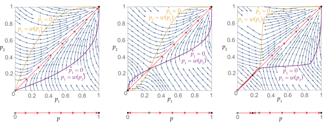
Figure A.1: Illustration of Equivalence Results for One- and Two-Population Dynamics

The figure illustrates the phase plots of three symmetric environments for two-population dynamics (upper panels) and the corresponding one-population dynamics (lower panels). Notice that the phase plots of one-population dynamics are similar to the part of phase plots of the corresponding two-population dynamics along the main diagonal (marked with red arrows). In all environments $u=2.4.$ In the left panels all agents have sample size $k=3$, in the middle panels all agents have sample size 7, and in the right panels $40\%$ of the agents have sample size 3, and $60\%$ have sample size 1000. Observe that in all cases, the dynamic predictions under both one-population dynamics and two-population dynamics are the same.

Proposition 5.

Let $(u,\theta)$ be a symmetric environment. State $(p_{1},p_{2})$ is asymptotically stable under two-population dynamics iff the state is symmetric (i.e., $p\equiv p_{1}=p_{2}$), and $p$ is asymptotically stable under one-population dynamics.

Proof.

From Proposition 4, it follows that all asymptotically stable states under two-population dynamics are symmetric. The strict monotonicity of $w$ implies that state $p$ satisfies conditions (1) and (2) in Fact 4 iff the symmetric state $(p,p)$ satisfies conditions (1) and (2) in Lemma 2. This, in turn, implies that state $p$ is asymptotically stable under one-population dynamics iff the symmetric state $(p,p)$ is asymptotically stable under two-population dynamics. ∎

A.3 General Result for Binomial Distributions

Recall our notation of $X(k,p)\sim Bin\left(k,p\right)$ denoting a random variable with binomial distribution, and of the function $F_{m}^{k}\left(p\right)\equiv\Pr\left(X\left(k,p\right)\geq m\right)$.

Proposition.

3 Fix arbitrary integers satisfying $0<m_{1}\leq k_{1}$ and $0<m_{2}\leq k_{2}$. There exists at most one $p\in\left(0,1\right)$ such that $\left(F_{m_{1}}^{k_{1}}\circ F_{m_{2}}^{k_{2}}\right)\left(p\right)=p$.

Proof.

Let $w_{i}\left(p\right)\equiv F_{m_{i}}^{k_{i}}\left(p\right)$ for each $i\in\left\{1,2\right\}$, $F\left(p\right)\equiv\left(F_{m_{1}}^{k_{1}}\circ F_{m_{2}}^{k_{2}}\right)\left(p\right)\equiv\left(w_{1}\circ w_{2}\right)\left(p\right),$ and $G\left(p\right)=F\left(p\right)-p$. In what follows we show that the function $G(\cdot)$ has at most one $p\in\left(0,1\right)$ such that $G\left(p\right)=0,$ which proves the result.

We have $G\left(0\right)=G\left(1\right)=0$. Assume to the contrary that there exist two different interior points $0<\underline{p}<\overline{p}<1$ such that $G\left(\underline{p}\right)=G\left(\overline{p}\right)$. Then $G$ equals zero at four points in the interval $\left[0,1\right]$. By Rolle’s theorem, this implies that $G^{\prime}$ is equal to zero in at least three points in the interval $\left(0,1\right),$ which further implies that $G^{\prime\prime}$ is equal to zero in at least two interior points in the interval $\left(0,1\right)$. Observe that $G^{\prime\prime}\equiv F^{\prime\prime}$. Thus, in order to obtain a contradiction we have to show that $F^{\prime\prime}\left(p\right)=0$ in at most one interior point. Recall that (see, e.g., Green, 1983, Eq. (5)):

$$w^{\prime}_{i}\left(p\right)=m_{i}\left(\begin{array}[]{c}k_{i}\\ m_{i}\end{array}\right)p^{m_{i}-1}\left(1-p\right)^{k_{i}-m_{i}}\,\Rightarrow\,\frac{w^{\prime\prime}_{i}\left(p\right)}{w^{\prime}_{i}\left(p\right)}=\frac{m_{i}-1}{p}-\frac{k_{i}-m_{i}}{1-p}.$$ (A.2)

For $p\in(0,1),$ using Eq. (A.2), we compute as follows:

$$F^{\prime}\left(p\right) =w_{1}^{\prime}\left(w_{2}\left(p\right)\right)w_{2}^{\prime}\left(p\right)$$

$$F^{\prime\prime}\left(p\right) =w_{1}^{\prime\prime}\left(w_{2}\left(p\right)\right)\left(w_{2}^{\prime}\left(p\right)\right)^{2}+w_{1}^{\prime}\left(w_{2}\left(p\right)\right)w_{2}^{\prime\prime}\left(p\right)$$

$$=w_{1}^{\prime}\left(w_{2}\left(p\right)\right)w_{2}^{\prime}\left(p\right)\left[\left(\frac{m_{1}-1}{w_{2}\left(p\right)}-\frac{k_{1}-m_{1}}{1-w_{2}\left(p\right)}\right)w_{2}^{\prime}\left(p\right)+\frac{m_{2}-1}{p}-\frac{k_{2}-m_{2}}{1-p}\right].$$

The fact that each $w_{i}\left(p\right)$ is strictly increasing implies that $F^{\prime\prime}\left(p\right)=0$ iff

$$\left(\frac{m_{1}-1}{w_{2}\left(p\right)}-\frac{k_{1}-m_{1}}{1-w_{2}\left(p\right)}\right)w_{2}^{\prime}\left(p\right)=\frac{k_{2}-m_{2}}{1-p}-\frac{m_{2}-1}{p}\Leftrightarrow$$

$$m_{2}\left(\begin{array}[]{c}k_{2}\\ m_{2}\end{array}\right)\left(\frac{m_{1}-1}{w_{2}\left(p\right)}-\frac{k_{1}-m_{1}}{1-w_{2}\left(p\right)}\right)p^{m_{2}-1}\left(1-p\right)^{k_{2}-m_{2}}=\frac{k_{2}-m_{2}}{1-p}-\frac{m_{2}-1}{p}\Leftrightarrow$$

$$\!\!\!\!\!\!\,\,\!\!m_{2}\left(\begin{array}[]{c}k_{2}\\ m_{2}\end{array}\right)\left(\frac{\left(m_{1}-1\right)p^{m_{2}}\left(1-p\right)^{k_{2}-m_{2}}}{\sum_{l=m_{2}}^{k_{2}}\left(\begin{array}[]{c}k_{2}\\ l\end{array}\right)p^{l}\left(1-p\right)^{k_{2}-l}}-\frac{\left(k_{1}-m_{1}\right)p^{m_{2}}\left(1-p\right)^{k_{2}-m_{2}}}{\sum_{l=0}^{m_{2}-1}\left(\begin{array}[]{c}k_{2}\\ l\end{array}\right)p^{l}\left(1-p\right)^{k_{2}-l}}\right)\frac{1}{p}=\frac{k_{2}-m_{2}}{1-p}-\frac{m_{2}-1}{p}\Leftrightarrow$$

$$m_{2}\left(\begin{array}[]{c}k_{2}\\ m_{2}\end{array}\right)\left(\frac{\left(m_{1}-1\right)}{\sum_{l=m_{2}}^{k_{2}}\left(\begin{array}[]{c}k_{2}\\ l\end{array}\right)\left(\frac{p}{1-p}\right)^{l-m_{2}}}-\frac{k_{1}-m_{1}}{\sum_{l=0}^{m_{2}-1}\left(\begin{array}[]{c}k_{2}\\ l\end{array}\right)\left(\frac{1-p}{p}\right)^{m_{2}-l}}\right)\frac{1}{p}=\frac{k_{2}-m_{2}}{1-p}-\frac{m_{2}-1}{p}$$

One could verify that the left-hand side of the above equation is strictly decreasing and the right-hand side is strictly increasing in $p.$ Therefore, there can be at most one point $p^{\ast}\in(0,1)$ where $F^{\prime\prime}(p^{\ast})=0.$ This completes the proof.∎

A.4 Standard Definitions of Dynamic Stability

For completeness, we present in this appendix the standard definitions of dynamic stability that are used in the paper (see, e.g., Weibull, 1997, Chapter 5).

A state is said to be stationary if it is a rest point of the dynamics.

Definition 4.

State $\mathbf{p}^{*}\in\left[0,1\right]^{2}$ is a stationary state if $w_{i}\left(\mathbf{p}^{*}\right)=p_{i}^{*}$ for each $i\in\left\{1,2\right\}$.

Let $\mathcal{E}\left(w\right)$ denote the set of stationary states of $w,$ i.e., $\mathcal{E}\left(w\right)=\{\mathbf{p}^{*}|w_{i}\left(\mathbf{p}^{*}\right)=p_{i}^{*}\}.$ Under monotone dynamics, an interior (mixed) state $\mathbf{p}^{*}\in(0,1)^{2}$ is a stationary state iff it is a Nash equilibrium (Weibull, 1997, Prop. 4.7). By contrast, under nonmonotone dynamics (such as the sampling dynamics analyzed below) the two notions differ.

A state $\mathbf{p}^{*}$ is Lyapunov stable if a population beginning near $\mathbf{p}^{*}$ stays close to it. $\mathbf{p}^{*}$ is asymptotically stable if it is Lyapunov stable and, in addition, nearby populations eventually converge to it. A state is unstable if it is not Lyapunov stable. It is well known (see, e.g., Weibull, 1997, Section 6.4) that every Lyapunov stable state must be a stationary state. Formally:

Definition 5.

A stationary state $\mathbf{p}^{*}\in\left[0,1\right]^{2}$ is Lyapunov stable if for every neighborhood $U$ of $\mathbf{p}^{*}$ there is a neighborhood $V\subseteq U$ of $\mathbf{p}^{*}$ such that if the initial state $p\left(0\right)\in V$, then $\mathbf{p}\left(t\right)\in U$ for all $t>0$. A state is unstable if it is not Lyapunov stable.

Definition 6.

A stationary state $\mathbf{p}^{*}\in\left[0,1\right]^{2}$ is asymptotically stable (or locally stable) if it is Lyapunov stable and there is some neighborhood $U$ of $\mathbf{p}^{*}$ such that all trajectories initially in $U$ converge to $\mathbf{p}^{*},$ i.e., $\mathbf{p}\left(0\right)\in U$ implies $\lim_{t\rightarrow\infty}\mathbf{p}\left(t\right)=\mathbf{p}^{*}$.

A.5 Proof of Proposition 1 (Stability of Pure States)

We are interested in deriving conditions for the stability of pure stationary states. In what follows, we compute the Jacobian of sampling dynamics in the pure state $\boldsymbol{a}=\left(0,0\right)$ (resp., $\boldsymbol{b}=\left(1,1\right)$). For this, we consider a slightly perturbed state with a “very small” $\epsilon_{i}$ share of agents playing $b_{i}$ (resp., $a_{i})$ in population $i$. By “very small,” we mean that higher-order terms of $\epsilon_{i}$ and $\epsilon_{j}$ are neglected.

Consider a new agent in population $i$ who has a sample size of $k_{i}.$ Action $b_{i}$ (resp., $a_{i}$) has a weakly (resp., strictly) higher mean payoff against a sample size of $k_{i}$ iff (neglecting rare events of having multiple $b_{j}$-s (resp., $a_{j}$-s) in the sample): (1) the sample includes the opponent’s action $b_{j}$ (resp., $a_{j}$), and (2) $k_{i}<\frac{1}{u_{i}}+1$ (resp., $k_{i}\leq u_{i}+1$). The probability of (1) is $k_{i}\cdot\epsilon_{j}+o(\epsilon_{j})$, where $o(\epsilon_{j})$ denotes terms that are sublinear in $\epsilon_{j}$, and, thus, it will not affect the Jacobian as $\epsilon_{j}\rightarrow 0$. This implies that the probability that a new agent in population $i$ (with a random sample size distributed according to $\theta_{i}$) who has a higher mean payoff for action $b_{i}$ (resp., $a_{i}$) against her sample is $w_{i}(1-\epsilon_{j})=\epsilon_{j}\cdot\mathbb{E}_{<\frac{1}{u_{i}}+1}\left(\theta_{i}\right)+o(\epsilon_{j})$ (resp., $w_{i}(\epsilon_{j})=\epsilon_{j}\cdot\mathbb{E}_{\leq u_{i}+1}\left(\theta_{i}\right)+o(\epsilon_{j})$ ). Therefore, the sampling dynamics at $(\epsilon_{1},\epsilon_{2})$ (resp., $(1-\epsilon_{1},1-\epsilon_{2})$) can be written as follows (ignoring the higher-order terms of $\epsilon_{1}$ and $\epsilon_{2}$):

$$\dot{\epsilon}_{i}=\epsilon_{j}\cdot\mathbb{E}_{<\frac{1}{u_{i}}+1}\left(\theta_{i}\right)-\epsilon_{i}\,\,\,(\textrm{resp.,}\,\dot{\epsilon}_{i}=\epsilon_{i}-\epsilon_{j}\cdot\mathbb{E}_{\leq u_{i}+1}\left(\theta_{i}\right)).$$ (A.3)

Define: $a_{\theta_{i}}=\mathbb{E}_{<\frac{1}{u_{i}}+1}\left(\theta_{i}\right)$ (resp., $b_{\theta_{i}}=\mathbb{E}_{\leq u_{i}+1}\left(\theta_{i}\right)$). The Jacobian of the above system of Equations (A.3) is then given by $J_{a}=\left(\begin{array}[]{cc}-1&a_{\theta_{1}}\\ a_{\theta_{2}}&-1\end{array}\right)$ (resp., $J_{a}=\left(\begin{array}[]{cc}1&-b_{\theta_{1}}\\ -b_{\theta_{2}}&1\end{array}\right)$). The eigenvalues of $J_{a}$ (resp., $J_{b}$) are $-1-\sqrt{a_{\theta_{1}}a_{\theta_{2}}}$ and $-1+\sqrt{a_{\theta_{1}}a_{\theta_{2}}}$ (resp., $-1-\sqrt{b_{\theta_{1}}b_{\theta_{2}}}$ and $-1+\sqrt{b_{\theta_{1}}b_{\theta_{2}}}$). Observe that: (1) if $a_{\theta_{1}}a_{\theta_{2}}<1$ (resp., $b_{\theta_{1}}b_{\theta_{2}}$>1) then both eigenvalues are negative, which implies that the pure state $\boldsymbol{a}$ (resp., $\boldsymbol{b}$) is asymptotically stable, and (2) if $a_{\theta_{1}}a_{\theta_{2}}>1$ (resp., $b_{\theta_{1}}b_{\theta_{2}}$>1) then one of the eigenvalues is positive, which implies that this state is unstable (see, e.g., Perko, 2013, Theorems 1 and 2 in Section 2.9).

A.6 Proof of Proposition 2

A.6.1 Proof of Claim 1 (Reaching the Area between the Curves)

We say that state p is above (resp., below) curve $w_{2}(p_{1})$ if $p_{2}>w_{2}(p_{1})$ (resp., ($p_{2}<w_{2}(p_{1})$). Similarly, we say that state p is to the right (resp., left) of the curve $w_{1}(p_{2})$ if $p_{1}>w_{1}(p_{2})$ (resp., $p_{1}<w_{1}(p_{2})$). We say that the state p is on the curve $w_{i}(p_{j})$ if $p_{i}=w_{i}(p_{j}).$ Due to the fact that the two curves are strictly increasing, we identify the notion of being above a curve and being to the left of the curve, and similarly we identify the notion of being below a curve and being to the right of the curve. The states on the curve $w_{2}(p_{1})$ (resp., $w_{1}(p_{2})$) are characterized by having $\dot{p_{2}}=0$ (resp., $\dot{p_{1}}=0$). Observe that $\dot{p_{2}}>0$ (resp., $\dot{p_{2}}<0$) in any state p above and to the left (resp., below and to the right) of the curve $w_{2}(p_{1})$. Similarly, $\dot{p_{1}}>0$ (resp., $\dot{p_{1}}<0$) in any state p above and to the left (resp., below and to the right) of the curve $w_{1}(p_{2})$.

Any state $\textbf{p}\in[0,1]$ can be classified in one of $9=3\cdot 3$ classes, depending on its relative location with respect to the two curves, i.e., whether p is below, above, or on each of the two curves $w_{i}(p_{j})$. If state p is on (resp., above, below) the curve $w_{2}(p_{1})$, then $\dot{p_{2}}$ is zero (resp., negative, positive). Similarly, if state p is on (resp., above, below) the curve $w_{1}(p_{2})$, then $\dot{p_{1}}$ is zero (resp., positive, negative). In particular, any state p that is above (resp., below) both curves must satisfy $\dot{p_{1}}>0>\dot{p_{2}}$. This implies that any trajectory that begins above (resp., below) both curves must always move downward and to the right. This (together with the fact that $\dot{\boldsymbol{p}}\left(t\right)=(0,0)$ only in the intersections of the two curves) implies that the trajectory must either converge to a stationary state (i.e., an intersection of the two curves), or cross one of the curves, and reach a state $\boldsymbol{p}\left(t\right)$ that satisfies either $w_{1}^{-1}\left(p_{1}\left(t\right)\right)\leq p_{2}\left(t\right)\leq w_{2}\left(p_{1}\left(t\right)\right)$ or $w_{2}\left(p_{1}\left(t\right)\right)\leq p_{1}\left(t\right)\leq w_{1}^{-1}\left(p_{1}\left(t\right)\right)$.

A.6.2 Proof of Claim 2 (Convergence to Stationary States)

We first show why we can assume w.l.o.g. that $\boldsymbol{p}\left(t\right)$ is strictly between the two curves. If $\boldsymbol{p}\left(t\right)$ crosses one of the curves and is strictly above (resp., below) the remaining curve, then the dynamics must take the populations to a state that is strictly below one of the curves and strictly above the remaining curve. This is so because on the crossing point one of the $\dot{p_{i}}$-s is zero and the remaining derivative $\dot{p}_{j}$ is negative (resp., positive), which implies that the dynamics take the trajectory below and to the right (resp., above and to the left) of the curve that was crossed.

Next assume that $p_{i}\left(t\right)\in\left(w_{1}^{-1}\left(p_{1}\left(t\right)\right),w_{2}\left(p_{1}\left(t\right)\right)\right)$ (resp., $p_{i}\left(t\right)\in\left(w_{2}\left(p_{1}\left(t\right)\right),w_{1}^{-1}\left(p_{1}\left(t\right)\right)\right).$ By the classification presented in the proof of Claim 1, the trajectory must move upward and to the right, i.e., $\dot{p_{1}},\dot{p_{2}}>0$ (resp., downward and to the left, i.e., $\dot{p_{1}},\dot{p_{2}}<0$). This implies that the trajectory must cross one of the curves. The crossing point cannot be only on the curve of $w_{2}(p_{1})$ (resp., $w_{1}(p_{2})$), because at such a point the trajectory moves horizontally to the left (vertically upward), which implies that it must cross the lower (resp., higher) curve $w_{2}(p_{1})$ (resp.,$w_{1}(p_{2})$) from the left side (resp., from below), and we get a contradiction. This implies that the crossing point must be the closest intersection points of the two curves to the right (resp., left) of $p_{i}\left(t\right)$, namely, $\overline{\boldsymbol{p}}$ (resp., $\boldsymbol{\underline{p}}$).

A.7 Proof of Lemma 1 (Convergence to Pure States)

If p is below (resp., above) both curves, then by the classification presented in the proof of Claim 1 it must be that $\dot{p_{2}}>0$ (resp., $\dot{p_{1}}>0$), which implies that convergence to (0,0) is possible only if the trajectory passes through a state that is strictly between the two curves, and that the closest intersection point of the two curves to the left of this state is (0,0). By the classification presented in the proof of Claim 2 it must be that the curve of $w_{2}(p_{1})$ is strictly below the curve of $w_{1}(p_{2})$ in a right neighborhood of (0,0), which implies that (0,0) is asymptotically stable because any sufficiently close initial state would converge to (0,0).

A.8 Proof of Lemma 2

Assume that Conditions (1) and (2) hold. Let $\boldsymbol{p}\neq\hat{\boldsymbol{p}}$ be any sufficiently close state. By Claim 1 any trajectory beginning at $\boldsymbol{p}$ will enter one of the two areas between the two curves on either side of $\hat{\boldsymbol{p}}$. By Claim 2, Condition (1) (resp., (2)) implies convergence to $\hat{\boldsymbol{p}}$ if the trajectory has entered the area between the curves to the left (resp., right) of $\hat{\boldsymbol{p}}.$ This implies that any trajectory that starts sufficiently close to $\hat{\boldsymbol{p}}$ must converge to $\hat{\boldsymbol{p}}$, and, thus, $\hat{\boldsymbol{p}}$ is asymptotically stable.

Next assume that $\hat{p}_{1}>0$ and Condition (1) (resp., $\hat{p}_{1}<1$ and Condition (2)) is not satisfied. This implies that $w_{2}\left(p_{1}\right)<w_{1}^{-1}\left(p_{1}\right)$ (resp., $w_{2}\left(p_{1}\right)>w_{1}^{-1}\left(p_{1}\right)$) for any $p_{1}$ that is sufficiently close to $\hat{p}_{1}$ from the left (resp., right). By Claim 2, this implies that a trajectory starting at $\left(p_{1},p_{2}\right)$ with $p_{1}$ sufficiently close to $\hat{p}_{1}$ from the left (resp., right) and with $p_{2}\in\left(w_{2}\left(p_{1}\right),w_{1}^{-1}\left(p_{1}\right)\right)$ (resp., $p_{2}\in\left(w_{1}^{-1}\left(p_{1}\right),w_{2}\left(p_{1}\right)\right)$) converges to the neighboring stationary point on the left (resp., right) side of $\hat{\boldsymbol{p}}$. Thus, $\hat{\boldsymbol{p}}$ is unstable.

A.9 Proof of Theorem 3 (Stability of Miscoordination)

Let $w_{i}^{k_{i}}\left(p_{j}\right)$ (resp., $w_{i}^{\theta_{i}}\left(p_{j}\right)$) denote the sampling dynamics induced by an agent with sample size $k_{i}$ (resp., agents with the distribution $\theta_{i}$).

1. Fix any $r<\min\left(\frac{1}{k_{1}},\frac{1}{k_{2}}\right)$. Assume that $u_{i}>\frac{1}{r}$ for each $i$ (which implies that $u_{i}>k_{i}$). Observe that

   $$w_{i}^{k_{i}}\left(p_{j}\right)=\Pr\left(X\left(k_{i},p_{j}\right)\geq 1\right)=1-\left(1-p_{j}\right)^{k_{i}}=k_{i}p_{j}-\left(\begin{array}[]{c}k_{i}\\ 2\end{array}\right)\left(p_{j}\right)^{2}+O\left(\left(p_{j}\right)^{3}\right).$$

   Fix a sufficiently small $\epsilon>0$. Let $\hat{p}_{1}\in\left(0,p_{1}^{NE}-\epsilon\right)$ be sufficiently small such that the term $O\left(\left(p_{j}\right)^{3}\right)<\epsilon$ is negligible for any $p_{j}<\hat{p}_{1}$. For each $i\in\left\{1,2\right\}$, let $\alpha_{i}\in\left(0,1\right)$ be such that: (1) $\alpha_{i}k_{i}>1$ and (2) $\alpha_{i}\left(k_{i}-\left(\begin{array}[]{c}k_{i}\\ 2\end{array}\right)p_{j}\right)<1-2\epsilon$. This implies that $w_{i}^{k_{i}}\left(p_{j}\right)>\frac{p_{j}}{\alpha_{i}}$ in a right neighborhood of zero, and $w_{i}^{k_{i}}\left(p_{j}\right)<\frac{p_{j}}{\alpha_{i}}$ in a left neighborhood of $\hat{p}_{1}$. Observe that $\lim_{k\rightarrow\infty}w_{2}^{k}\left(\hat{p}_{1}\right)=0$ and $\lim_{k\rightarrow\infty}\left(w_{1}^{k}\right)^{-1}\left(\hat{p}_{1}\right)=p_{2}^{NE}$. This implies that there exists $\overline{k}$ sufficiently large such that $w_{2}^{\overline{k}}\left(\hat{p}_{1}\right)<\epsilon$ and $\left(w_{1}^{\overline{k}}\right)^{-1}\left(\hat{p}_{1}\right)>p_{2}^{NE}-\epsilon>\hat{p}_{1}$. Observe that $w_{i}^{k_{i}\alpha_{i}\overline{k}}\left(p_{j}\right)>p_{j}$ in a right neighborhood of zero, and $w_{i}^{k_{i}\alpha_{i}\overline{k}}\left(p_{j}\right)<p_{j}$ in a left neighborhood of $\hat{p}_{1}$. This, in turn, implies that $w_{2}^{k_{2}\alpha_{2}\overline{k}}\left(p_{1}\right)>p_{1}>\left(w_{1}^{k_{2}\alpha_{2}\overline{k}}\right)^{-1}\left(p_{1}\right)$ in a right neighborhood of zero, and $w_{2}^{k_{2}\alpha_{2}\overline{k}}\left(p_{1}\right)<p_{1}<\left(w_{1}^{k_{1}\alpha_{1}\overline{k}}\right)^{-1}\left(p_{1}\right)$ in a left neighborhood of $\hat{p}_{1}$. Thus, there exists a stationary state $\tilde{\boldsymbol{p}}$ that satisfies $0<\tilde{p}_{1}<\hat{p}_{1}<1$, and $w_{2}^{k_{i}\alpha_{i}\overline{k}}\left(p_{1}\right)>\left(w_{1}^{k_{i}\alpha_{i}\overline{k}}\right)^{-1}\left(p_{1}\right)$ (resp., $w_{2}^{k_{i}\alpha_{i}\overline{k}}\left(p_{1}\right)<\left(w_{1}^{k_{i}\alpha_{i}\overline{k}}\right)^{-1}\left(p_{1}\right)$) in a left (resp., right) neighborhood of $\tilde{p}_{1}$. This implies, by Claim 2, that $\tilde{\boldsymbol{p}}$ is asymptotically stable. The argument in this case is illustrated in the left panel of Figure 6.1.

2. Observe that

   $$w_{1}^{k_{1}}\left(p_{2}\right)=\Pr\left(\textrm{a new agent in population 1 has at least one }a_{2}\textrm{ in her sample}\right)$$

   is the same for all values of $u_{1}>k_{1}$, and, similarly,

   $$w_{2}^{k_{2}}\left(p_{1}\right)=\Pr\left(\textrm{a new agent in population 2 has no }b_{1}\textrm{-s}\right.\left.\textrm{in the sample}\right)$$

   is the same for all values of $u_{2}<\frac{1}{k_{2}}$. Fix a sufficiently small $\epsilon>0$. Let $\bar{u}_{1}>k_{1},\bar{u}_{2}<\frac{1}{k_{2}}$ be payoffs satisfying $p_{2}^{NE}=\frac{1}{1+\bar{u}_{1}}<\frac{w_{2}^{k_{2}}\left(\frac{1}{2}\right)}{2}-\epsilon$ and $1-p_{1}^{NE}=\frac{\bar{u}_{2}}{1+\bar{u}_{2}}<\frac{1-w_{1}^{k_{1}}\left(\frac{1}{2}\right)}{2}-\epsilon$. Let $r=\min\left(\frac{1}{1+\bar{u}_{1}},\frac{\bar{u}_{2}}{1+\bar{u}_{2}}\right)$. Fix any payoff profile $u_{1}>\frac{1}{r}$ and $u_{2}<r$. Let $\overline{k}$ be sufficiently large such that $w_{i}^{\overline{k}}\left(p_{j}^{NE}-\epsilon\right)<\epsilon$, $w_{i}^{\overline{k}}\left(p_{j}^{NE}+\epsilon\right)>1-\epsilon$. In what follows, we show that the environment $\left((u_{1},u_{2}),(k_{1}\frac{1}{2}\bar{k},k_{2}\frac{1}{2}\bar{k})\right)$ admits an asymptotically stable interior state (i.e., we let $\alpha_{1}=\alpha_{2}=\frac{1}{2}$).
   By Proposition 1, the two pure equilibria are asymptotically stable and $w_{2}^{k_{2}\frac{1}{2}\bar{k}}\left(p_{1}\right)<\left(w_{1}^{k_{1}\frac{1}{2}\bar{k}}\right)^{-1}\left(p_{1}\right)$ (resp., $w_{2}^{k_{2}\frac{1}{2}\bar{k}}\left(p_{1}\right)>\left(w_{1}^{k_{1}\frac{1}{2}\bar{k}}\right)^{-1}\left(p_{1}\right)$) in a right (resp., left) neighborhood of zero (resp., one). Next observe that $w_{2}^{k_{2}\frac{1}{2}\bar{k}}\left(\frac{1}{2}\right)>\frac{1}{2}w_{2}^{k_{2}}\left(\frac{1}{2}\right)>p_{NE}^{2}+\epsilon>\left(w_{1}^{k_{1}\frac{1}{2}\bar{k}}\right)^{-1}\left(\frac{1}{2}\right)$, which implies that there is an (unstable) interior stationary state $\hat{\boldsymbol{p}}$ that satisfies: (1) $\hat{p}_{1}<0.5$, (2) $p_{NE}^{2}-\epsilon<\hat{p}_{2}<p_{NE}^{2}+\epsilon<0.5$, and (3) $w_{2}^{k_{2}\frac{1}{2}\bar{k}}\left(p_{1}\right)>\left(w_{1}^{k_{1}\frac{1}{2}\bar{k}}\right)^{-1}\left(p_{1}\right)$ in a right neighborhood of $\hat{p}_{1}$. By an analogous argument, there is also an (unstable) interior stationary state $\tilde{\boldsymbol{p}}$ that satisfies: (1) $\tilde{p}_{2}>0.5$, (2) $p_{1}^{NE}-\epsilon<\tilde{p}_{1}<p_{1}^{NE}+\epsilon<0.5$, and (3) $w_{2}^{k_{2}\frac{1}{2}\bar{k}}\left(p_{1}\right)<\left(w_{1}^{k_{1}\frac{1}{2}\bar{k}}\right)^{-1}\left(p_{1}\right)$ in a left neighborhood of $\tilde{p}_{1}$. This implies that must be an interior stationary state $\grave{\boldsymbol{p}}$ between $\hat{\boldsymbol{p}}$ and $\tilde{\textbf{p}}$ such that $w_{2}^{k_{2}\frac{1}{2}\bar{k}}\left(p_{1}\right)>\left(w_{1}^{k_{1}\frac{1}{2}\bar{k}}\right)^{-1}\left(p_{1}\right)$ (resp., $w_{2}^{k_{2}\frac{1}{2}\bar{k}}\left(p_{1}\right)>\left(w_{1}^{k_{1}\frac{1}{2}\bar{k}}\right)^{-1}\left(p_{1}\right)$) in a left (resp., right) neighborhood of $\grave{\boldsymbol{p}}$. Finally, Claim 2 implies that $\grave{\boldsymbol{p}}$ is asymptotically stable.

References

- Arieli et al. (2020) Arieli, I., Y. Babichenko, R. Peretz, and H. P. Young (2020). The speed of innovation diffusion in social networks. Econometrica 88(2), 569–594.
- Arigapudi et al. (2021) Arigapudi, S., Y. Heller, and I. Milchtaich (2021). Instability of defection in the prisoner’s dilemma under best experienced payoff dynamics. Journal of Economic Theory 197, 105174.
- Bilancini et al. (2022) Bilancini, E., L. Boncinelli, S. Ille, and E. Vicario (2022). Memory retrieval and harshness of conflict in the hawk–dove game. Economic Theory Bulletin 10(2), 333–351.
- Brunner et al. (2011) Brunner, C., C. F. Camerer, and J. K. Goeree (2011). Stationary concepts for experimental 2 2 games: Comment. American Economic Review 101(2), 1029–1040.
- Cárdenas et al. (2015) Cárdenas, J., C. Mantilla, and R. Sethi (2015). Stable sampling equilibrium in common pool resource games. Games 6(3), 299–317.
- Crawford (1989) Crawford, V. P. (1989). Learning and mixed-strategy equilibria in evolutionary games. Journal of Theoretical Biology 140(4), 537–550.
- Danenberg and Spiegler (2022) Danenberg, T. and R. Spiegler (2022). Representative sampling equilibrium. Working Paper.
- Fudenberg and Levine (1995) Fudenberg, D. and D. K. Levine (1995). Consistency and cautious fictitious play. Journal of Economic Dynamics and Control 19(5–7), 1065–1089.
- Genesove and Mayer (2001) Genesove, D. and C. Mayer (2001). Loss aversion and seller behavior: Evidence from the housing market. Quarterly Journal of Economics 116(4), 1233–1260.
- Goeree et al. (2003) Goeree, J. K., C. A. Holt, and T. R. Palfrey (2003). Risk averse behavior in generalized matching pennies games. Games and Economic Behavior 45(1), 97–113.
- Green (1983) Green, D. N. (1983). Fixed point properties of the binomial function. Journal of the Franklin Institute 316(1), 51–62.
- (12) Harsanyi, J. C. and R. Selten. A General Theory of Equilibrium Selection in Games. MIT Press.
- Hauert and Miekisz (2018) Hauert, C. and J. Miekisz (2018). Effects of sampling interaction partners and competitors in evolutionary games. Physical Review E 98(5), 052301.
- Heller (2017) Heller, Y. (2017). Instability of belief-free equilibria. Journal of Economic Theory 168, 261–286.
- Heller and Mohlin (2018) Heller, Y. and E. Mohlin (2018). Social learning and the shadow of the past. Journal of Economic Theory 177, 426–460.
- Herold and Kuzmics (2020) Herold, F. and C. Kuzmics (2020). The evolution of taking roles. Journal of Economic Behavior & Organization 174, 38–63.
- Kandori et al. (1993) Kandori, M., G. J. Mailath, and R. Rob (1993). Learning, mutation, and long run equilibria in games. Econometrica 61(1), 29–56.
- Kaniovski and Young (1995) Kaniovski, Y. M. and H. P. Young (1995). Learning dynamics in games with stochastic perturbations. Games and Economic Behavior 11(2), 330–363.