NAI₂: Learning Noise-Aware Illuminance-Interpolator for Unsupervised Low-Light Image Enhancement

Abstract

Low-light situations severely restrict the pursuit of aesthetic quality in consumer photography. Although many efforts are devoted to designing heuristics, it is generally mired in a shallow spiral of tedium, such as piling up complex network architectures and empirical strategies. How to delve into the essential physical principles of illumination compensation has been neglected. Following the way of simplifying the complexity, this paper innovatively proposes a simple and efficient Noise-Aware Illumination Interpolator (NAI₂). According to the constraint principle of illuminance and reflectance within a limited dynamic range, as a prior knowledge in the recovery process, we construct a learnable illuminance interpolator and thereby compensating for non-uniform lighting. With the intention of adapting denoising without annotated data, we design a self-calibrated denoiser with the intrinsic image properties to acquire noiseless low-light images. Starting from the properties of natural image manifolds, a self-regularized recovery loss is introduced as a way to encourage more natural and realistic reflectance map. The model architecture and training losses, guided by prior knowledge, complement and benefit each other, forming a powerful unsupervised leaning framework. Comprehensive experiments demonstrate that the proposed algorithm produces competitive qualitative and quantitative results while maintaining favorable generalization capability in unknown real-world scenarios. The code will be available online upon publication of the paper.

Figure 1: Comparison among recent state-of-the-art unsupervised methods, including ZeroDCE (Guo et al. 2020), RetinexDIP (Zhao et al. 2021), RUAS (Liu et al. 2021a), and SCI (Ma et al. 2022). The left subfigure displays the numerical scores obtained for image enhancement on the LOL dataset (Wei et al. 2018) and segmentation on the Dark Zurich dataset (Sakaridis, Dai, and Gool 2019). The right subfigures display the enhanced images, estimated illumination maps, and error maps generated by the corresponding retinex-based methods.

Introduction

The boom in smartphones and advanced photography has catalyzed the quest for aesthetic image quality for both shooters and viewers. Nevertheless, because of severe backlighting conditions or technical limitations (e.g., insufficient light and limited exposure time), images captured in low-light conditions often exhibit poor visual quality (e.g., low visibility, low contrast, chromatic aberration, intense noise, etc.). Over the past few years, researchers have made considerable efforts in developing the conversion of low-quality low-illumination imagery to normally exposed high-quality imagery, i.e., Low-Light Image Enhancement (LLIE). It has broad application prospects for downstream machine analytics, such as for consumer photography (Liba et al. 2019), autonomous driving (Wang et al. 2022), and video surveillance (Potter et al. 2020).

Over the past few decades, extensive attention has been focused on the study of image recovery tailored for underlit environments. From earlier classical manually designed algorithms (Jobson, Rahman, and Woodell 1997; Rahman, Jobson, and Woodell 1996) to more recent data-driven deep models (Ignatov et al. 2017; Lv et al. 2018; Yang et al. 2020a), researchers have made considerable efforts and yielded favorable effects in enhancing the visual quality of low-light observations. However, existing LLIE methods are caught in a tedious and complex empirical vortex. Some methods introduce large-scale network models (Ma et al. 2021), or complex learning strategies (Jiang et al. 2021; Liu et al. 2021b; Zhang et al. 2021), which improve visual quality but still remain in the black box of divorced prior knowledge. To eliminate the dependence on paired training data, unsupervised LLIE is emerging as a hot research area of interest to scholars. Some unsupervised learning algorithms are capable of restoring images with good illumination and contrast in some cases. However, most approaches either rely heavily on elaborate network architectures (Li et al. 2021), exploit well-chosen diversified losses (Guo et al. 2020; Jiang et al. 2021), or construct multi-stage tedious strategies (Ma et al. 2022; Guo et al. 2020). Even more, a few unsupervised enhancement models (Ma et al. 2022) neglect the noise problem of low-illumination images, and inevitably produce amplified noise in darker regions.

Training an unsupervised neural network using only regularization and fidelity terms to enhance low-light images is challenging due to uneven illumination and complex textures. Most regularization terms in unsupervised loss are inaccurate in modeling prior knowledge and cannot meet the assumptions of the illumination map or reconstruction results, requiring extensive tuning to find optimal parameters. This leads to unpredictable enhancement and an uninterpretable network.

To address these issues, we estimate image noise level and propose a noise aware denoiser to remove noise before enhancement for better performance. Additionally, we design a learnable illuminance interpolator that structurally satisfies common assumptions about illumination, making the network interpretable. Moreover, we have designed a loss function that is simpler and more intuitive in structure compared to common unsupervised loss functions. By directly constraining the brightness range of the output, the enhancement results are predictable. The main contributions are summarized as follows:

• We propose a self-calibrated denoising approach that incorporates precise noise estimation, enabling the generation of low-light images that are both smooth and edge-preserving. Our method significantly improves enhancing performance on a diverse range of datasets.

• We construct a learnable illumination interpolator for learning a global smooth but structure aware illumination representation for LLIE problems. Thereby without smoothing and fidelity loss, it can still generate an illumination map that satisfies the spatial assumption naturally.

• Starting from the properties of natural image manifolds, a self-regularized recovery loss is introduced as a way to encourage more natural and realistic reflectance map. The model architecture and training losses, guided by prior knowledge, complement and benefit each other, forming a powerful unsupervised leaning framework.

Related works

Figure 2: Illustrations of the fundamental components for NAI₂. Top: (a) Self-Calibrated Denoiser, (b) Learnable Illuminance Interpolator. Bottom: (c) Denoise Module $\mathcal{N}_{d}(\mathbf{x},\bm{\omega_{d}})$, (d) Illuminance Learning Module $\mathcal{M}_{i}(\mathbf{x},\bm{\omega_{i}})$, (e) Conditional Feature Modulation (CFM) Right: (f) Key operations.

In the realm of low-light image enhancement (LLIE), researchers have delved into an assortment of network models aimed at tackling the amalgamation of degradation factors and improving representations. RetinexNet(Wei et al. 2018) introduced a semi-decoupled approach comprising a Decom-Net for decomposition and an Enhance-Net for illumination adjustment. MBLLEN(Lv et al. 2018) employed a deep learning method with multi-branch fusion to extract features from various levels and enhance low-light images through multiple subnets. GLADNet(Wang et al. 2018) dealt with LLIE via a Global illumination Aware and Detail-preserving Network. RUAS(Liu et al. 2021a) employed a collaborative reference-free learning searching strategy to discover a suitable network architecture for enhancing low-light images, obviating the need for handcrafting design. However, while the proposed methods aim to achieve a better network architecture, relationships between components are frequently excluded from the network, impeding the learning of the enhancing prior and rendering the network uninterpretable.

Besides, numerous training strategies have been explored for LLIE to investigate the relationship between low-light and normal images. DRBN (Yang et al. 2020a) presented a semi-supervised learning approach utilizing deep recursive band networks to extract coarse-to-fine band representations and reconstitute towards high-quality images. ZeroDCE (Guo et al. 2020) estimated pixel-wise and high-order curves for dynamic range adjustment of a given image using a lightweight deep network. EnGAN (Jiang et al. 2021) introduced a global-local discriminator structure, self-regularized perceptual loss fusion, and attention mechanism to train the network in an adversarial way without paired images. RetinexDIP (Zhao et al. 2021) devised a novel ”generative” strategy for Retinex decomposition and a unified deep framework for low-light image enhancement, without external image data. SCI (Ma et al. 2022) put forward a new self-calibrated illumination learning framework to reduce computational cost and accelerate the training process. Nonetheless, these intricate strategies are proposed indirectly, necessitating handcrafted tuning for each term and rendering the network’s outputs unpredictable.

Methodology

First-Denoising Last-Illuminance-Learning

Motivated by the Retinex theory (Land 1977), we adapt a more general framework for low-light imaging that accounts for incidental compatible noise. The framework can be formulated as $\mathbf{x}=\mathbf{y}\otimes\mathbf{s}+\mathbf{v}$, where $\mathbf{x}$ denotes the low-light input corrupted by incidental noise $\mathbf{v}$, $\mathbf{s}$ represents the reflectance, $\mathbf{y}$ represents the illumination, and $\otimes$ denotes the element-wise product operation.

Prior work in simultaneous noise and illumination removal can be broadly classified into two categories: one involves denoising in a separate reflectance branch, while the other performs denoising directly after obtaining the reflectance result. The former involves the aggregation of the reflection and illumination branches, while the latter yields a sharp output. In contrast, our approach offers a new perspective by first removing noise from the low-light image itself, followed by illumination learning. This method adheres to the physical principles of low-light imaging and decouples the tasks of noise removal and illumination learning, distinguishing it from most previous work which considers denoising in the reflectance.

Specifically, we construct an unsupervised learning framework with noise removal followed by illuminance learning, including a precursor Self-Calibrated Noise Remover (SNR) and a subsequent Learnable Illumination Interpolator (LII). The learning paradigm can be formulated as follows:

$$\mathtt{SNR-to-LII}:\left\{\begin{aligned} \mathbf{u}&=\mathbf{x}-\mathbf{v},~{}\mathtt{where}~{}\mathbf{v}=\mathcal{N}_{d}(\mathbf{x};\bm{\omega_{d}}),\\ \mathbf{s}&=\mathbf{u}\oslash\mathbf{y},~{}\mathtt{where}~{}\mathbf{y}=\mathcal{M}_{i}(\mathbf{u};\bm{\omega_{i}}),\end{aligned}\right.$$ (1)

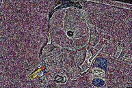
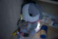
where $\mathcal{N}_{d}$ and $\mathcal{M}_{i}$ denote the noise removal module and illumination learning module, parameterized by $\bm{\omega_{d}}$ and $\bm{\omega_{i}}$, respectively. $\mathbf{v}$ and $\mathbf{u}$ denote the noise map and noiseless low-light map, respectively. For further understanding, a visualization of the intermediate results regarding the workflow is illustrated in Figure 3.

Input: $\mathbf{x}$	Noise: $\mathbf{v}$	Illumination: $\mathbf{y}$	Reflectance: $\mathbf{s}$

Figure 3: Visualization of intermediate results (i.e., $\mathbf{x}$, $\mathbf{v}$, $\mathbf{y}$ and $\mathbf{s}$) regarding the workflow of NAI₂ based on Eq (1).

Self-Calibrated Noise Remover

Capturing nighttime images naturally flooded with large amount of noise distracts the visual perception, hence noise removal is an indispensable part for unsupervised low-light recovery. In the following, we attempt to explore the noise intensity distribution of low-light input from its intrinsic properties (e.g., gradient information), and develop a self-calibrated noise remover to bootstrap the image to remove the intrinsic noise in an unsupervised manner.

Theorem 1.

The gradient characteristics of image can reflect the distribution of potential noise. Thus, we use the higher order gradient of the image to estimate the noise intensity. After a rigorous theoretical derivation the following equation is given :

$$\sigma\approx\psi(\nabla^{n}\mathbf{x}):=\frac{\sqrt{\pi}E|\nabla^{n}\mathbf{x}|}{\sqrt{2\Sigma_{k=0}^{n}[C_{n}^{k}]^{2}}}.$$ (2)

Here, $\nabla^{n}\mathbf{x}$ represents the $n$-order image gradient. Given an image with pixel coordinate position $p$, the gradient can be computed as $\nabla\mathbf{x}(p)=\mathbf{x}(p)-\mathbf{x}(p+1)$, and for $n>1$, it can be calculated recursively using $\nabla^{n}\mathbf{x}(p)=\nabla^{n-1}\mathbf{x}(p)-\nabla^{n-1}\mathbf{x}(p+1)$.

As shown in (c) of Figure 2, SNR can be formulated as

$$\mathcal{N}_{d}(\mathbf{x};\bm{\omega_{d}}):\left\{\begin{aligned} \bm{f_{\sigma}}&={\mathcal{F}}_{CFT}\left({\mathcal{F}}_{conv}(\sigma)\right),\\ \mathbf{v}&=\mathcal{G}(\sigma,\sigma_{g})\otimes{\mathcal{F}}_{Unet}\left({\mathcal{F}}_{C}\big{(}\bm{f_{\sigma}},\mathbf{x}\big{)}\right),\end{aligned}\right.$$ (3)

Specifically, the noise level $\bm{\sigma}$ is estimated based on Equation (8), which in turn is embedded into the conditional feature transformation layer ${\mathcal{F}}_{CFT}$ to obtain the latent feature map $\bm{f_{\sigma}}$. The details of the operation ${\mathcal{F}}_{CFT}$ are displayed in (e) of Figure 2. Further, the cascaded raw input $\mathbf{x}$ is fed to the Unet-style based denoiser ${\mathcal{F}}_{Unet}$ with a noise gate function $\mathcal{G}$ to estimate the noise map $\mathbf{v}$. The function can be formulated as $\mathcal{G}(\sigma,\sigma_{g})=sign(relu(\sigma-\sigma_{g}))$ to regulate the procedure, ensuring the preservation of critial details and preventing over-smoothing when dealing with noiseless images.

Learnable Illuminance Interpolator

Retinex theory resolves the ill-posed problem of isolating the illumination from the reflection in a given image, thus compensating for the inhomogeneous illumination. As a matter of fact, we generalize the following uniform prior knowledge. It reflects the physical laws about the original input, illumination and reflection that need to be satisfied in a limited dynamic range.

Remark 1.

Dynamic Range Constraint: Imposing the normalization operation restriction to raw input, the reflectance and illumination in the limited dynamic range during recovery satisfy the following prior constraints: $0\leq\mathbf{x}\leq\mathbf{s}\leq\mathbf{e},$ and $0\leq\mathbf{x}\leq\mathbf{y}\leq\mathbf{e}.$ Due to the potential structural consistency between $\mathbf{x}$, $\mathbf{s}$ and $\mathbf{y}$, the problem of separating illumination from reflectance in a given image, inspired by retinex theory , can be addressed by constructing an explicit interpolation operator/function.

Based on the above remark, we argue that the most intuitive idea to estimate illumination $\mathbf{y}$ is to build the linear interpolation function $g(\mathbf{x})$, denoted as $\mathbf{y}=g(\mathbf{x})\otimes\mathbf{x}+(\mathbf{e}-g(\mathbf{x})).$ It is worth noting that, here we experimentally observe that a certain enhancement effect can be obtained by constructing the interpolation function $g(\mathbf{x})$ with respect to the image mean $\mathtt{Mean}$ , denoted as $g(\mathbf{x})=\mathbf{e}-\mathtt{Mean}(\mathbf{x})$.

To further improve the representational capability and the nonlinear nature of the function of $g$, we construct learnable network module $\mathcal{M}_{i}(\mathbf{u},\bm{\omega_{i}})$ (parameterized by $\bm{\omega_{i}}$) to simulate the process of illumination generation in the form of interpolation. Specifically, the noise-free low-light image $\mathbf{u}$ are transmitted to the network to generate illumination factors and then illumination is calculated in a weighted form. The above illuminance learning process is formulated as

$$\mathbf{y}=\mathbf{u}\otimes\bm{\alpha}~{}+~{}\mathbf{e}\otimes\bm{\beta},~{}\mathtt{where}~{}\{\bm{\alpha},\bm{\beta}\}\leftarrow\mathcal{M}_{i}(\mathbf{u},\bm{\omega_{i}}),$$ (4)

where $\mathbf{e}$ denotes the unit matrix. $\bm{\alpha}$ and $\bm{\beta}$ are the learned illuminance interpolation map, equal in magnitude to the original input $\mathbf{x}$. In the implementation phase, we specify that the learned illumination factors satisfy $\bm{\alpha}+\bm{\beta}=\mathbf{e}$, resulting in a natural structure constraint on fidelity and smooth properties of illumination. As shown in (d) of Figure 2, $\mathcal{M}_{i}(\mathbf{u},\bm{\omega_{i}})$ is constructed as a network module. We will delve into the compelling advantages of LII with such structure constraint in Section Discussion 4.

Reference-Free Loss Function

The total loss function is expressed as

$$\mathcal{L}_{total}={\lambda}_{srr}*\mathcal{L}_{srr}+{\lambda}_{nr}*\mathcal{L}_{nr},$$ (5)

where $\mathcal{L}_{srr}$ and $\mathcal{L}_{nr}$ are self-regularized recovery loss, and noise removal loss respectively. ${\lambda}_{srr}$ and ${\lambda}_{nr}$ are the corresponding weights.

Self-Regularized Recovery Loss. Inspired by the gray world assumption and following normal image’s pixel intensity distribution, we propose the self-regularized recovery loss $\mathcal{L}_{srr}$ to encourage color naturalness of the result and it can be formulated as

$$\mathcal{L}_{srr}(\mathbf{s})=e^{relu(|\bar{\mathbf{s}}-\eta_{1}|-\eta_{2})}-1,$$ (6)

where $\bar{\mathbf{s}}$ is the mean value of image $\mathbf{s}$ in different channels, $\eta_{1}$ and $\eta_{2}$ are constants, and presents the mean and standard deviation value of the desired enhanced image. $\eta_{1}$ is set to $[0.485,0.456,0.406]$ and $\eta_{2}$ is set to $[0.229,0.224,0.225]$ according to statistical laws of Imagenet (Deng et al. 2009). Further discussion is provided in Section Discussion 6.

Self-Adaptable Noise Removal Loss. To preserve edge details during the denoising process, we introduce an adaptive denoising loss function that dynamically balances the weights of fidelity term and regularization term (Rudin, Osher, and Fatemi 1992), thereby ensuring optimal performance across varying noise intensities encountered in unsupervised denoising. It can be formulate as

$$\mathcal{L}_{nr}(\mathbf{y})=||\mathbf{u}-\mathbf{x}||^{2}+\eta*\sigma(\mathbf{x})*\mathtt{TV}(\mathbf{u}),$$ (7)

in which the regularized term $\mathtt{TV}$ is the standard total variation with a hyper- parameter $\eta>0$, and the noise coefficient $\sigma(\mathbf{x})$ is the noise aware weight for balancing the smoothness and details of the input $\mathbf{x}$, estimated by the Equation (8).

Table 1: Quantitative comparison on MIT and LOL dataset regarding two full-reference metrics (i.e., PSNR and SSIM) and two no-reference metrics (i.e., LOE and NIQE).

Data	Metric	Supervised Learning Methods				Unsupervised Learning Methods
		Retinex	GLADNet	DRBN	MBLLEN	EnGAN	ZeroDCE	RetinexDIP	RUAS	SCI †	Ours
MIT	PSNR$\uparrow$	12.7337	16.1199	16.2923	17.5187	15.3634	15.9995	17.8654	12.2772	17.3501	18.6832
	SSIM$\uparrow$	0.592	0.6443	0.6064	0.6156	0.6331	0.6649	0.7164	0.5985	0.6649	0.6890
	LOE$\downarrow$	1820.1250	261.9865	737.1467	184.6337	849.4681	496.2076	505.8833	878.7199	225.2516	104.0570
	NIQE$\downarrow$	4.3868	3.9207	4.7097	5.2657	3.8452	3.6777	3.812	6.5968	4.0352	3.9812
LOL	PSNR$\uparrow$	16.3076	19.6969	18.2622	17.6662	17.6844	16.4015	12.5299	14.9663	15.8407	20.3721
	SSIM$\uparrow$	0.4362	0.6555	0.6688	0.5767	0.6081	0.5731	0.5048	0.4986	0.5193	0.7183
	LOE$\downarrow$	1030.256	374.2944	615.3503	367.5218	529.2202	227.4783	386.8785	377.3417	124.8404	356.2606
	NIQE$\downarrow$	10.2436	7.4375	5.4802	5.4660	5.5585	8.8945	8.8192	7.8084	8.9301	5.4132

Discussion

Figure 4: Visual comparison of estimated illumination map. Left: Combination reference produced by the ground truth, Right: Illuminance estimated via reverse procedure (i.e., $\mathbf{x}\oslash\mathbf{s}$).

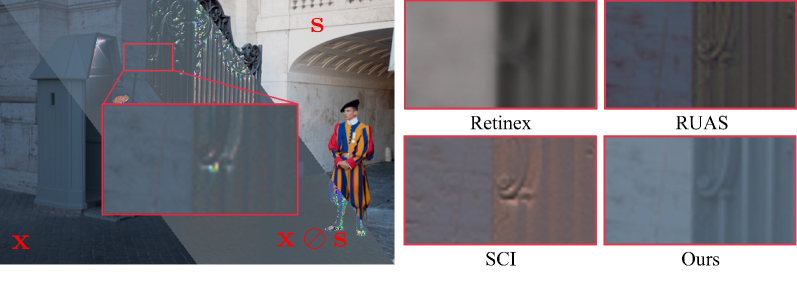
Charm of Illuminance Interpolator.   Compared to Retinex-induced LLIE methods, the proposed illuminance interpolator learns a difference function from the original image to the illuminance map. With its advanced interpolation structure, the LII naturally satisfies the assumptions for illumination smoothing and structural fidelity. On the one hand, combined with the luminance-oriented loss function, the interpolation process reduces the gap between pixels and achieves smoothing of illuminated image regions, and edge preservation. On the other hand, without introducing additional constraints on the illumination map and without tediously considering the effect of the coefficients between the fidelity and regularity terms on the enhancement results, this facilitates fast optimization iterations on different datasets. Note that comparison results of the Retinex-induced LLIE methods is illustrated in Figure 4. Considering the Retinex-induced model, we calculate the illumination map $\mathbf{y}$ of various methods by using $\mathbf{x}\oslash\mathbf{s}$. Obviously, the illumination map estimated by our NAI₂ is smoother and retains the edge detail information of the original image. Details of the experiments can be found in the supplementary materials.

Figure 5: Statistic results of estimated illumination map. Our illumination maps’ distribution outperforms at least as well as other retinex-based methods, despite without using corresponding loss explicitly.

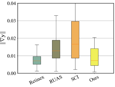LII provides a natural way to ensure the fidelity and smooth assumption of illumination and our loss draws a desired blueprint of the final result’s properties. Although without constrained directly on illumination map as other retinex-based methods do, our method outperforms at least as well as other retinex-based approaches. We quantitatively analyze illumination maps by measuring the common constraint term $\|\nabla\mathbf{y}\|$ and the translated fidelity term $\|\hat{\mathbf{x}}-\hat{\mathbf{y}}\|^{2}$, where $\hat{\mathbf{x}}=\mathbf{x}-\mathtt{Mean}(\mathbf{x})$ and $\hat{\mathbf{y}}=\mathbf{y}-\mathtt{Mean}(\mathbf{y})$. We use the MIT dataset for our experiment to avoid interference from noise. Results in Figure 5 show that our method produces smoother and more similar illumination maps to the low-light input.

Figure 6: Charm of self-regularized recovery loss for robust enhancement. $\mathbf{s_{i}}$ presents the enhanced result of $\mathbf{x_{i}}$ and $\mathbf{\Delta s}=10(\mathbf{s_{1}-s_{2}})^{2}$ means scaled square difference between results for better comparison. Mean square error are listed at the bottom to quantify the difference of similar inputs/results.

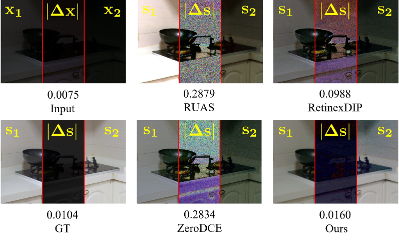
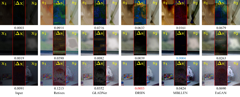
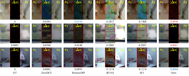
Charm of Self-Regularized Recovery Loss. The loss ensures that the brightness of each channel is constrained within a small margin, similar to normal images. If the brightness is at a normal level, the loss will be zero, but if it is over-exposed or under-exposed, the loss will increase rapidly. From the perspective of image manifold, this approach considers mapping the high-dimensional information of the image into a low-dimensional manifold region that reflects the color distribution of the image, allowing us to effectively enhance low-light images without over-exposure or under-exposure. Additionally, the color loss function permits the efficient optimization of parameters without the need for complex, prior-based domain knowledge, with LLI’s linear convex interpolation structure. Compared to other methods that require adjusting hyper parameters between distinct loss terms, our novel illumination architecture utilizes only the color loss function, thus simplifying the training process. Moreover, when handling low-light images with subtle differences, our proposed method generates results that exhibit smaller differences compared to other approaches. This outcome further validates the robustness, as shown in Figure 6.

EXPERIMENTAL RESULTS

Input	Retinex	GLADNet	DRBN	MBLLEN	EnGAN
Reference	ZeroDCE	RetinexDIP	RUAS	SCI	Ours

Figure 7: Visual results of state-of-the-art LLIE methods and ours on the MIT dataset. Zoom in for best view.

Implementation Details

All the experiments were conducted on PC with the TITAN RTX GPU and Intel(R) Core(TM) i9-10940X CPU @ 3.30GHz.

Benchmark Datasets and Evaluation Metrics. Our proposed method was rigorously evaluated on two widely adopted low-light image enhancement datasets, namely MIT (Bychkovsky et al. 2011) and LOL (Wei et al. 2018), as well as on a recently introduced dataset, Dark Zurich (Sakaridis, Dai, and Gool 2019), for nighttime semantic segmentation. To evaluate the effectiveness of our approach, we employed two full-reference metrics (i.e., PSNR and SSIM (Wang et al. 2004)) as well as no-reference metrics (i.e., LOE (Wang et al. 2013) and NIQE (Mittal, Soundararajan, and Bovik 2013)) to comprehensively assess the performance of low-light image enhancement. For the semantic segmentation task, we adopt three full-reference metrics (i.e., aAcc, mIoU, and mAcc).

Training Configuration. In the training process, we performed unsupervised learning on each dataset. The images were first clipped into patches with a size of $128\times 128$ and a batch size of $16$ was used. We utilized Adam optimizer with an initial learning rate of $1\times 10^{-4}$ and betas of $0.9$ and $0.999$ in our experiment. We employed alternating optimization of SNR and LLI. Specifically, in each loop, LLI was updated 50 times followed by 50 updates to SNR. The model was trained within 4000 iterations

Benchmark Evaluation

We performed quantitative and qualitative evaluations of the proposed method against several state-of-the-art LLIE methods, including supervised learning methods (i.e., Retinex (Wei et al. 2018), GLADNet (Wang et al. 2018), DRBN (Yang et al. 2020a) and MBLLEN (Lv et al. 2018)), and unsupervised learning methods (i.e, EnGAN (Jiang et al. 2021), ZeroDCE (Guo et al. 2020), RetinexDIP (Zhao et al. 2021), RUAS (Liu et al. 2021b), and SCI  (Ma et al. 2022) ).

Quantitative evaluation. Table 1 reports quantitative comparison results on the MIT and LOL datasets. As can be seen, our method numerically outperforms existing unsupervised learning methods and even supervised learning methods by a large margin and ranks first in almost all metrics. In comparison to the second-best unsupervised state-of-the-art method on the MIT dataset, our approach achieves a PSNR improvement of 0.8178dB. Furthermore, when compared to the best performing supervised method, our approach results in a PSNR improvement of 1.1645dB. Likewise, on the LOL dataset, our method leads to improvements of 2.6877dB and 1.2752dB, respectively. Benefiting from the systematic network architecture and reference-free loss we construct, our method outperforms the results of existing unsupervised methods and supervised learning methods on both MIT and LOL datasets significantly.

Qualitative evaluation. Qualitative results are displayed in Figures 7. As illustrated, previous efforts did not achieve the desired enhancement results, resulting in inconspicuous details, unnatural colors and overexposure or underexposure. In contrast, our NAI₂ achieves the best visual quality with vivid colors and outstanding texture details.Due to space limitations, more visual comparisons are available in the supplemental materials.

Computational Efficiency. Our proposed method is characterized by high efficiency . Specifically, the model size is only 7.7046M, and the GPU runtime is 0.0096s. At full speed, our method can perform high-performance enhancement at a rate of up to 100 frames per second.

High-level Applications

Nighttime Semantic Segmentation. We utilized the segmentation model PSPNet (Zhao et al. 2017) to investigate the performance of enhancement results on downstream nighttime semantic segmentation task. In the context of semantic segmentation, we investigated the cross-domain semantic segmentation of urban roads from day to night. The segmentation network PSPNet was trained on the Cityscapes dataset (Cordts et al. 2016) and tested on the validation set of Dark Zurich. With the exception of RetinexDIP, all methods utilized training weights from the MIT or LOL dataset to enhance low-light images and subsequently underwent semantic segmentation testing using PSPNet. Quantitative results are presented in Table 2 and more visual results are available in supplemental materials. Ours is better It can be seen that our method numerically outperforms existing LLIE methods by large margins and shows favorable segmentation capability while preserving sharp structures in terms of sidewalk and background trees.

Table 2: Quantitative segmentation comparison regarding aAcc (%) $\uparrow$, mIOU (%) $\uparrow$ and mAcc (%) $\uparrow$ on Dark-Zurich dataset.

Metric	RUAS	SCI	RetinexDIP	ZeroDCE	Ours
aAcc$\uparrow$	26.27	33.79	35.75	44.55	47.97
mIoU$\uparrow$	6.69	7.38	9.06	10.65	13.22
mAcc$\uparrow$	15.49	16.00	19.39	19.61	24.79

Ablation Studies

We conducted ablation studies to investigate individual network components, executive order and reference-free loss functions.

Effects of SNR and LII. Table 3 presents the results of network module (i.e., SNR and LII) ablation on the LOL dataset. It should be noted that in the table, [M1] refers to the model without the SNR module, and [M2] represents the removal of the LII module, which is replaced by the unsupervised illumination learning network proposed in the recent work SCI (Ma et al. 2022). We observe that without the SNR module, the performance decreased by $2.1901dB$ and $0.2008$ on the PSNR and SSIM metrics, respectively. Moreover, the substitution of LII for SCI significantly attenuates the performance on all metrics, especially with a $5.1061dB$ decrease in PSNR. We argue that the root cause of this phenomenon is that the substituted Model [M2] does not comply with the loss optimization procedure under the illumination prior constraint condition with a simple loss function. In the other hand, it indicates that our LII module satisfy the illumination prior naturally.

Table 3: Ablation study toward network modules (i.e., SNR and LII) on LOL dataset.

Method	PSNR$\uparrow$	SSIM$\uparrow$	LOE$\downarrow$	NIQE$\downarrow$
Config.: M1 (w/o SNR), M2 (w/o LII, w/SCI),
M3 (w/o $\psi(\nabla^{n}\mathbf{x})$), M4 (LII-to-SNR)
M1	18.1820	0.5175	195.1463	8.7650
M2	15.2660	0.5162	1277.8000	5.8762
M3	20.0589	0.7009	373.0177	5.1661
M4	19.2083	0.6783	418.1006	4.8808
Ours	20.3721	0.7183	356.2606	5.4132

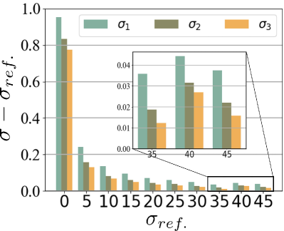
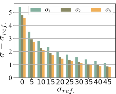
High-Order Gradient-Based Noise Estimator. To verify the effectiveness of using the higher-order gradient of images to estimate the image noise intensity $\bm{\sigma}$, we randomly selected 10 low-light images on the MIT dataset and 10 normal images on the LOL dataset, respectively. On this basis, we then randomly added Gaussian noise with noise intensity $\bm{\sigma}_{ref.}$ and estimated the noise intensity $\bm{\sigma}_{n}$ using a noise estimator of order $n$ (i.e., $n=1,2,3$). The process was repeated 100 times for each image. As shown in Figure 8, the noise estimation accuracy increases with increasing noise intensity and also with increasing order of the image gradient used. The experiments prove that the 1-st order noise estimator remains high accuracy for high intensity noise($1\%$ error when sigma is greater than 20 in low-light images), and therefore the experiment defaults to the 1st order noise estimator. Having examined the accuracy of the noise estimator, we subsequently investigate its influence on the enhanced results. To be specific, we remove the noise estimator from denoiser and formulated Model [M3] for experimental purposes, as shown in Table 3. The outcomes reveal that the noise estimator can proficiently eliminate noise and boost the performance of our approach.

MIT dark images	LOL normal images

Figure 8: Ablation study of high-order gradient-based noise estimator on MIT dark images and LOL normal images.

SNR-to-LII v.s. LII-to-SNR. We explore the effects of executive order of SNR, and construct model [M4] where its front LII is spliced with a post-processor denoiser plug-in. The corresponding quantitative is reported in Table 3, showing that using “SNR-to-LII” improves the performance of LLIE to a certain extent on three performance metrics, compared with “LII-to-SNR”.

Table 4: Ablation study regarding the proposed reference-free loss (i.e., $\mathcal{L}_{srr}and\mathcal{L}_{nr}$) on LOL dataset.

Method	SNR	$\mathcal{L}_{DCE}$	$\mathcal{L}_{SCI}$	$\mathcal{L}_{srr}$	$\mathcal{L}_{TV}$	$\mathcal{L}_{nr}$	PSNR$\uparrow$	SSIM$\uparrow$
M5		✓					10.8484	0.2553
M6			✓				10.5643	0.2835
M7				✓			18.1820	0.5175
M8	✓			✓	✓		20.1610	0.6023
Ours	✓			✓		✓	20.3721	0.7183

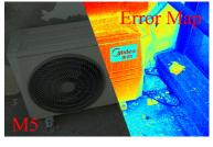
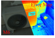
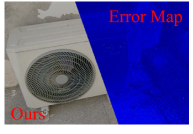
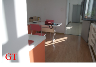
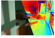
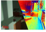
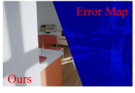
Exploration on Reference-Free Loss. Our study investigates the effectiveness of self-regularized recovery loss in comparison with popular unsupervised learning loss functions, including $\mathcal{L}_{DCE}$ from ZeroDCE (Guo et al. 2020) and $\mathcal{L}_{SCI}$ from SCI (Ma et al. 2022), as shown in Table 4. We built Model [M5] and [M6] separately using the corresponding complex loss configurations. Hyperparameters of the loss functions are utilized without any coefficient adjustment for evaluate its robustness. However, due to the lack of a denoising function of these model, we remove the $\mathcal{L}_{nr}$ as well as SNR term and construct Model [M7] for justice. None of the models include an SNR module. Our quantitative results show a substantial improvement in Model [M7] over Models [M5] and [M6], such as a $67.6\%$ PSNR score improvement, demonstrating robustness and effectiveness in color restoration, as indicated in Figure 9 and Table 4. Additionally, we explore self-adaptable noise removal loss by removing the adaptive factor $\sigma(\mathbf{x})$ from $\mathcal{L}_{nr}$ to train Model [M8], which leads to the degradation of the loss to the most common denoise loss $\mathcal{L}_{TV}$ (Rudin, Osher, and Fatemi 1992). Our final model shows improvements in the PSNR and SSIM metrics of $0.2111dB$ and $0.1160$, respectively.

—	(13.615, 0.620)	(13.657, 0.611)	(22.389, 0.754)
—	(10.421, 0.340)	(10.323, 0.368)	(24.779, 0.7614)

Figure 9: Ablation study on the impact of reference-free loss. (PSNR$\uparrow$, SSIM$\uparrow$) are listed at the bottom to quantify the generated image quality, and a scaled heatmap of the square error between ground truth and result is concatenated to the right part of enhanced image for better comparison.

Conclusion

Drawing inspiration from the retinex theory’s partitioning scheme, we present a structure-constrained noise-aware illumination interpolator, coupled with a reference-free loss function that is intuitive yet effective. Our network’s interpretability and the predictability of the enhanced results are attributed to the utilization of these simple yet effective approaches. In various datasets, our proposed method outperforms state-of-the-art methods in most metrics. Moreover, the enhanced results generated by our approach exhibit excellent performance when applied to other low-light datasets, thereby facilitating high-level visual tasks, such as segmentation.

Supplementary Materials for
”NAI₂: Learning Noise-Aware Illuminance-Interpolator for Unsupervised Low-Light Image Enhancement”

Appendix A Proof for Noise Estimation

Theorem 2.

The gradient characteristics of image can reflect the distribution of potential noise. Thus, we use the higher order gradient of the image to estimate the noise intensity. After a rigorous theoretical derivation the following equation is given:

$$\sigma\approx\psi(\nabla^{n}\mathbf{x}):=\frac{\sqrt{\pi}E|\nabla^{n}\mathbf{x}|}{\sqrt{2\Sigma_{k=0}^{n}[C_{n}^{k}]^{2}}}.$$ (8)

Here, $\nabla^{n}\mathbf{x}$ represents the $n$-order image gradient. Given an image with pixel coordinate position $p$, the gradient can be computed as $\nabla\mathbf{x}(p)=\mathbf{x}(p)-\mathbf{x}(p+1)$, and for $n>1$, it can be calculated recursively using $\nabla^{n}\mathbf{x}(p)=\nabla^{n-1}\mathbf{x}(p)-\nabla^{n-1}\mathbf{x}(p+1)$.

Proof.

Here we initially consider the Gaussian noise distribution $\mathbf{v}\sim\mathcal{N}(0,\sigma^{2})$ with a standard deviation of $\sigma$, and define the following relationship: $\mathbf{x}=\mathbf{u}+\mathbf{v}$ between the noisy input $\mathbf{x}$ and noise-free image $\mathbf{u}$. First, we define the first-order gradient and $n$-order gradient ($n>1$) of the image at pixel coordinate position $p$, i.e., $\nabla\mathbf{x}(p)=\mathbf{x}(p)-\mathbf{x}(p+1)$ and $\nabla^{n}\mathbf{x}(p)=\nabla^{n-1}\mathbf{x}(p)-\nabla^{n-1}\mathbf{x}(p+1)$. Decoupling the noise map $\mathbf{v}$ and clear images $\mathbf{u}$, we obtain $\nabla^{n}\mathbf{x}(p)=\nabla^{n}\mathbf{u}(p)+\nabla^{n-1}\mathbf{v}(p)-\nabla^{n-1}\mathbf{v}(p+1)$. Recursively, we further obtain $\nabla^{n}\mathbf{x}(p)=\nabla^{n}\mathbf{u}(p)+T$, where $T=\Sigma_{k=0}^{n}(-1)^{k}C_{n}^{k}\mathbf{v}(p+k).$ Since each noisy pixel is independently and identically distributed, i.e., $\mathbf{v}(p)\sim\mathcal{N}(0,\sigma^{2})$, we have $T\sim\mathcal{N}(0,\Sigma_{k=0}^{n}[C_{n}^{k}]^{2}\sigma^{2})$ and $E|T|=\sigma\sqrt{\frac{2}{\pi}\Sigma_{k=0}^{n}[C_{n}^{k}]^{2}}$, where $E$ denotes the expectation sign.

Further, according to $E|\nabla^{n}\mathbf{x}|=E|\nabla^{n}\mathbf{u}+T|$, we can obtain the following inequality: $E|T|-E|\nabla^{n}\mathbf{u}|\leq E|\nabla^{n}\mathbf{x}|\leq E|T|+E|\nabla^{n}\mathbf{u}|.$ Since the natural noise-free image satisfies the smoothness property, the following rules are satisfied $\nabla\mathbf{u}(p_{s})\rightarrow 0$ and $\nabla\mathbf{u}(p_{e})\rightarrow\mathbf{u}(p_{e})$ for the smooth region pixel point $p_{s}$ and the edge pixel point $p_{e}$. Further we obtain $E|\nabla^{n}\mathbf{u}|\approx E|\nabla\mathbf{u}|$. Substituting into the inequality, we have $E|T|-E|\nabla\mathbf{u}|\leq E|\nabla^{n}\mathbf{x}|\leq E|T|+E|\nabla\mathbf{u}|$. When $n$ is large enough, $E|\nabla^{n}\mathbf{u}|\approx E|\nabla\mathbf{u}|=const\ll\sqrt{\Sigma_{k=0}^{n}[C_{n}^{k}]^{2}}$, $E|\nabla^{n}\mathbf{u}|\ll E|T|$, it follows from the pinch-force theorem that $E|\nabla^{n}\mathbf{x}|\approx E|T|=\sigma\sqrt{\frac{2}{\pi}\Sigma_{k=0}^{n}[C_{n}^{k}]^{2}}.$ Therefore, the Gaussian noise intensity can be estimated by statistical analysis of $|\nabla^{n}\mathbf{x}|$, which yields $\sigma\approx\psi(\nabla^{n}\mathbf{x}):=\frac{\sqrt{\pi}E|\nabla^{n}\mathbf{x}|}{\sqrt{2\Sigma_{k=0}^{n}[C_{n}^{k}]^{2}}}$. ∎

Appendix B Interpolation Function

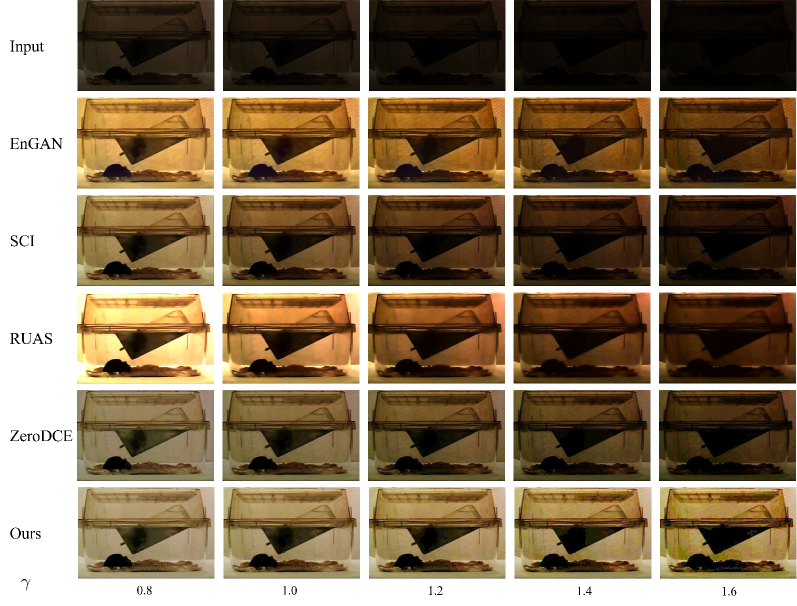
Based on the remark 1 in the Methodology part, we argue that the most intuitive idea to estimate illumination $\mathbf{y}$ is to build the linear interpolation function $g(\mathbf{x})$, denoted as $\mathbf{y}=g(\mathbf{x})\otimes\mathbf{x}+(\mathbf{e}-g(\mathbf{x})).$ It is worth noting that, here we experimentally observe that a certain enhancement effect can be obtained by constructing the interpolation function $g(\mathbf{x})$ with respect to the image mean $\mathtt{Mean}$, denoted as $g(\mathbf{x})=\mathbf{e}-\mathtt{Mean}(\mathbf{x})$. As shown in Figure 10, the simplest function (InterRes) has ability to enhance images with different degradation factors. Though InterRes shows its robustness to light condition change, it is still lack of adaptability to different scenarios. And the proposed LLI framework learns an interpolation map and inherits its robustness against the slight changes of environments, as Figure LABEL:robust_enhancement reveals.

Figure 10: Degraded inputs and enhanced results with different $\gamma$ factors. InterRes means results with the simplest interplation function $g(\mathbf{x})$ with respect to the image mean $\mathtt{Mean}$.

Figure 11: Robust enhancement towards different similar images in LOL dataset. $\mathbf{s_{i}}$ presents the enhanced result of $\mathbf{x_{i}}$ and $\mathbf{\Delta s}=10(\mathbf{s_{1}-s_{2}})^{2}$ means scaled square difference between results for better comparison. Mean square error are listed at the bottom to quantify the difference of similar inputs/results. The best result is in red whereas the second best one is in blue.

Table 5: The model size, FLOPs and running time (GPU-seconds for inference) of unsupervised learning methods and our NAI₂.

	EnGAN	ZeroDCE	RUAS	SCI	LII	Ours
SIZE (M)	8.6366	0.0794	0.0034	0.0002	0.0017	7.7046
TIME (S)	0.0032	0.0014	0.0045	0.0002	0.0055	0.0096

Appendix C More Experimental Details on Different Datasets

Input	RUAS	RetinexDIP	ZeroDCE	SCI	Ours

Figure 12: Visual results of state-of-the-art LLIE methods and ours on the Dark-Zurich dataset. Zoom in for best view.

Input	EnGAN	ZeroDCE	RetinexDIP
RUAS	SCI	Ours	OursRe

Figure 13: Visual results of state-of-the-art LLIE methods and ours on the Darkface dataset. Note all methods are tested directly except method Ours_Re, which is retrained on Darkface. Zoomed-in areas indicate obvious differences.

Enhancement on LOL

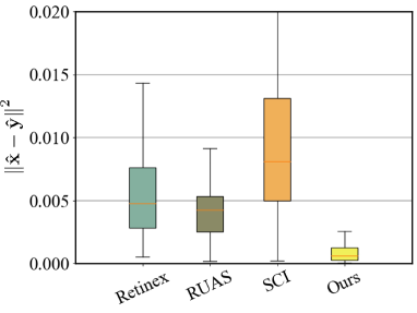
We random selected 99 images from LOL (Wei et al. 2018) dataset as test set, and utilize the rest to train different models. In LOL dataset, images with different light conditions in the same scenario are provided, and many of them are slight different with each other. Despite the minor variations in the input images, achieving stable appearance including pixel intensity remains a challenge. To address this problem, we evaluate a range of state-of-the-art unsupervised methods, such as EnGAN (Jiang et al. 2021), ZeroDCE (Guo et al. 2020), RetinexDIP (Zhao et al. 2021), RUAS (Liu et al. 2021b), and SCI (Ma et al. 2022), as well as supervised methods, including Retinex (Wei et al. 2018), GLADNet (Wang et al. 2018), DRBN (Yang et al. 2020a), and MBLLEN (Lv et al. 2018). We select pairs of images in test set with similar content captured under different lighting conditions. Additionally, we use mean square error as the metric to compare the enhanced images and results are revealed in Figure 11. Our method consistently achieves the lowest differences among the unsupervised methods and outperforms most of the supervised methods. Specifically, our proposed method generates results with smaller differences compared to other approaches when handling low-light images with subtle differences. This finding further validates the robustness of our approach and its ability to defend against slight changes while producing stable results.

Enhancement on Dark Zurich

In this section, our focus is on exploring the ability of image enhancement on a specific dataset, namely the Dark Zurich Validation Set (Sakaridis, Dai, and Gool 2019). To ensure fair comparison with similar network parameters and computation cost, our approach does not involve hyper-parameter finetuning, and we only use the LII module for enhancement. Even in the absence of the SNR module, our proposed LII demonstrates superior performance, as evidenced by the results presented in Figure 12. We observe that existing methods, such as RUAS, ZeroDCE, and SCI, produce over-exposed results without external finetuning or early stop strategies. Although RetinexDIP exhibits better visual performance, its iterative optimization process is too time-consuming to achieve real-time enhancement speeds. In contrast, our approach is both fast and flexible, and delivers highly effective results. We achieve real-time enhancement without the need for external finetuning or early stop strategies, and demonstrate superior performance compared to existing methods.

Enhancement on Darkface

In this section, we tested models on Darkface (Yang et al. 2020b). To show our proposed method’s robustness, compared methods as well as ours were trained on MIT and tested on Darkface directly except Ours_Re to provide a direct trained result for comparison. Note that the relevant experiments on Darkface are based only on the constructed learnable illumination interpolator module, demonstrating the superiority of the proposed LII even in the absence of SNR.

Appendix D Model Size and Computation Efficiency

In Table 5, we report the model size, FLOPs, and running time (in GPU-seconds) of some recently proposed CNN-based methods. Our method only requires 7.7046M parameters, and the GPU runtime is 0.0096s. As a result, our method can achieve high-performance enhancement at a rate of up to 100 frames per second, enabling real-time enhancement speed. While our approach may be slightly slower than other methods, it still achieves a fast enough speed given the limitations of the recording speed of general devices. Moreover, our approach delivers higher visual performance, resulting in a better view.

References

- Bychkovsky et al. (2011) Bychkovsky, V.; Paris, S.; Chan, E.; and Durand, F. 2011. Learning photographic global tonal adjustment with a database of input/output image pairs. In CVPR 2011, 97–104. IEEE.
- Cordts et al. (2016) Cordts, M.; Omran, M.; Ramos, S.; Rehfeld, T.; Enzweiler, M.; Benenson, R.; Franke, U.; Roth, S.; and Schiele, B. 2016. The cityscapes dataset for semantic urban scene understanding. In Proceedings of the IEEE conference on computer vision and pattern recognition, 3213–3223.
- Deng et al. (2009) Deng, J.; Dong, W.; Socher, R.; Li, L.-J.; Li, K.; and Fei-Fei, L. 2009. Imagenet: A large-scale hierarchical image database. In 2009 IEEE conference on computer vision and pattern recognition, 248–255. Ieee.
- Guo et al. (2020) Guo, C.; Li, C.; Guo, J.; Loy, C. C.; Hou, J.; Kwong, S.; and Cong, R. 2020. Zero-reference deep curve estimation for low-light image enhancement. In Proceedings of the IEEE/CVF conference on computer vision and pattern recognition, 1780–1789.
- Ignatov et al. (2017) Ignatov, A.; Kobyshev, N.; Timofte, R.; Vanhoey, K.; and Van Gool, L. 2017. Dslr-quality photos on mobile devices with deep convolutional networks. In Proceedings of the IEEE international conference on computer vision, 3277–3285.
- Jiang et al. (2021) Jiang, Y.; Gong, X.; Liu, D.; Cheng, Y.; Fang, C.; Shen, X.; Yang, J.; Zhou, P.; and Wang, Z. 2021. Enlightengan: Deep light enhancement without paired supervision. IEEE transactions on image processing, 30: 2340–2349.
- Jobson, Rahman, and Woodell (1997) Jobson, D. J.; Rahman, Z.-u.; and Woodell, G. A. 1997. A multiscale retinex for bridging the gap between color images and the human observation of scenes. IEEE Transactions on Image processing, 6(7): 965–976.
- Land (1977) Land, E. H. 1977. The retinex theory of color vision. Scientific american, 237(6): 108–129.
- Li et al. (2021) Li, J.; Li, J.; Fang, F.; Li, F.; and Zhang, G. 2021. Luminance-Aware Pyramid Network for Low-Light Image Enhancement. IEEE Transactions on Multimedia, 23: 3153–3165.
- Liba et al. (2019) Liba, O.; Murthy, K.; Tsai, Y.-T.; Brooks, T.; Xue, T.; Karnad, N.; He, Q.; Barron, J. T.; Sharlet, D.; Geiss, R.; Hasinoff, S. W.; Pritch, Y.; and Levoy, M. 2019. Handheld Mobile Photography in Very Low Light. ACM Trans. Graph., 38(6).
- Liu et al. (2021a) Liu, R.; Ma, L.; Zhang, J.; Fan, X.; and Luo, Z. 2021a. Retinex-inspired Unrolling with Cooperative Prior Architecture Search for Low-light Image Enhancement. In CVPR.
- Liu et al. (2021b) Liu, R.; Ma, L.; Zhang, J.; Fan, X.; and Luo, Z. 2021b. Retinex-inspired unrolling with cooperative prior architecture search for low-light image enhancement. In Proceedings of the IEEE/CVF Conference on Computer Vision and Pattern Recognition, 10561–10570.
- Lv et al. (2018) Lv, F.; Lu, F.; Wu, J.; and Lim, C. 2018. MBLLEN: Low-Light Image/Video Enhancement Using CNNs. In BMVC, volume 220, 4.
- Ma et al. (2021) Ma, L.; Liu, R.; Zhang, J.; Fan, X.; and Luo, Z. 2021. Learning deep context-sensitive decomposition for low-light image enhancement. IEEE Transactions on Neural Networks and Learning Systems, 33(10): 5666–5680.
- Ma et al. (2022) Ma, L.; Ma, T.; Liu, R.; Fan, X.; and Luo, Z. 2022. Toward fast, flexible, and robust low-light image enhancement. In Proceedings of the IEEE/CVF Conference on Computer Vision and Pattern Recognition, 5637–5646.
- Mittal, Soundararajan, and Bovik (2013) Mittal, A.; Soundararajan, R.; and Bovik, A. C. 2013. Making a “Completely Blind” Image Quality Analyzer. IEEE Signal Processing Letters, 20(3): 209–212.
- Potter et al. (2020) Potter, M.; Gridley, H.; Lichtenstein, N.; Hines, K.; Nguyen, J.; and Walsh, J. 2020. Low-Light Environment Neural Surveillance. In 30th IEEE International Workshop on Machine Learning for Signal Processing, MLSP 2020, Espoo, Finland, September 21-24, 2020, 1–6. IEEE.
- Rahman, Jobson, and Woodell (1996) Rahman, Z.; Jobson, D. J.; and Woodell, G. A. 1996. Multi-scale retinex for color image enhancement. In Proceedings 1996 International Conference on Image Processing, Lausanne, Switzerland, September 16-19, 1996, 1003–1006. IEEE Computer Society.
- Rudin, Osher, and Fatemi (1992) Rudin, L. I.; Osher, S.; and Fatemi, E. 1992. Nonlinear total variation based noise removal algorithms. Physica D: nonlinear phenomena, 60(1-4): 259–268.
- Sakaridis, Dai, and Gool (2019) Sakaridis, C.; Dai, D.; and Gool, L. V. 2019. Guided curriculum model adaptation and uncertainty-aware evaluation for semantic nighttime image segmentation. In Proceedings of the IEEE/CVF International Conference on Computer Vision, 7374–7383.
- Wang et al. (2022) Wang, H.; Chen, Y.; Cai, Y.; Chen, L.; Li, Y.; Sotelo, M. A.; and Li, Z. 2022. SFNet-N: An Improved SFNet Algorithm for Semantic Segmentation of Low-Light Autonomous Driving Road Scenes. IEEE Transactions on Intelligent Transportation Systems, 23(11): 21405–21417.
- Wang et al. (2013) Wang, S.; Zheng, J.; Hu, H.-M.; and Li, B. 2013. Naturalness Preserved Enhancement Algorithm for Non-Uniform Illumination Images. IEEE Transactions on Image Processing, 22(9): 3538–3548.
- Wang et al. (2018) Wang, W.; Wei, C.; Yang, W.; and Liu, J. 2018. Gladnet: Low-light enhancement network with global awareness. In 2018 13th IEEE international conference on automatic face & gesture recognition (FG 2018), 751–755. IEEE.
- Wang et al. (2004) Wang, Z.; Bovik, A. C.; Sheikh, H. R.; and Simoncelli, E. P. 2004. Image quality assessment: from error visibility to structural similarity. IEEE transactions on image processing, 13(4): 600–612.
- Wei et al. (2018) Wei, C.; Wang, W.; Yang, W.; and Liu, J. 2018. Deep retinex decomposition for low-light enhancement. arXiv preprint arXiv:1808.04560.
- Yang et al. (2020a) Yang, W.; Wang, S.; Fang, Y.; Wang, Y.; and Liu, J. 2020a. From fidelity to perceptual quality: A semi-supervised approach for low-light image enhancement. In Proceedings of the IEEE/CVF conference on computer vision and pattern recognition, 3063–3072.
- Yang et al. (2020b) Yang, W.; Yuan, Y.; Ren, W.; Liu, J.; Scheirer, W. J.; Wang, Z.; Zhang; and et al. 2020b. Advancing Image Understanding in Poor Visibility Environments: A Collective Benchmark Study. IEEE Transactions on Image Processing, 29: 5737–5752.
- Zhang et al. (2021) Zhang, R.; Guo, L.; Huang, S.; and Wen, B. 2021. ReLLIE: Deep reinforcement learning for customized low-light image enhancement. In Proceedings of the 29th ACM international conference on multimedia, 2429–2437.
- Zhao et al. (2017) Zhao, H.; Shi, J.; Qi, X.; Wang, X.; and Jia, J. 2017. Pyramid Scene Parsing Network. In CVPR.
- Zhao et al. (2021) Zhao, Z.; Xiong, B.; Wang, L.; Ou, Q.; Yu, L.; and Kuang, F. 2021. RetinexDIP: A unified deep framework for low-light image enhancement. IEEE Transactions on Circuits and Systems for Video Technology, 32(3): 1076–1088.