Long-term predictions of turbulence by implicit U-Net enhanced Fourier neural operator
Abstract
Long-term predictions of nonlinear dynamics of three-dimensional (3D) turbulence are very challenging for machine learning approaches. In this paper, we propose an implicit U-Net enhanced Fourier neural operator (IU-FNO) for stable and efficient predictions on the long-term large-scale dynamics of turbulence. The IU-FNO model employs implicit recurrent Fourier layers for deeper network extension and incorporates the U-net network for the accurate prediction on small-scale flow structures. The model is systematically tested in large-eddy simulations of three types of 3D turbulence, including forced homogeneous isotropic turbulence (HIT), temporally evolving turbulent mixing layer, and decaying homogeneous isotropic turbulence. The numerical simulations demonstrate that the IU-FNO model is more accurate than other FNO-based models including vanilla FNO, implicit FNO (IFNO) and U-Net enhanced FNO (U-FNO), and dynamic Smagorinsky model (DSM) in predicting a variety of statistics including the velocity spectrum, probability density functions (PDFs) of vorticity and velocity increments, and instantaneous spatial structures of flow field. Moreover, IU-FNO improves long-term stable predictions, which has not been achieved by the previous versions of FNO. Besides, the proposed model is much faster than traditional LES with DSM model, and can be well generalized to the situations of higher Taylor-Reynolds numbers and unseen flow regime of decaying turbulence.
I Introduction
Neural networks (NNs) have been widely applied to improve or replace the conventional modeling of turbulent flows in computational fluid dynamics (CFD).Brunton, Noack, and Koumoutsakos (2020); Duraisamy, Iaccarino, and Xiao (2019); Liu et al. (2020); Vignon, Rabault, and Vinuesa (2023); Zuo et al. (2023) Various strategies based on NNs have been developed to enhance Reynolds-averaged Navier-Stokes simulation (RANS) and large-eddy simulation (LES) of turbulence.Maulik et al. (2018); Yuan et al. (2021); Wang et al. (2021); Beck, Flad, and Munz (2018); Xie et al. (2019); Wang et al. (2018); Sarghini, De Felice, and Santini (2003); Gamahara and Hattori (2017); Zhou et al. (2019); Li et al. (2021a); Guan et al. (2022); Ling, Kurzawski, and Templeton (2016); Tabe Jamaat and Hattori (2023) Beck et al. proposed convolutional neural networks (CNNs) and residual neural networks (RNNs) to construct accurate subgrid-scale (SGS) models for LES.Beck, Flad, and Munz (2019) Zhou et al. used an artificial neural network to develop a new SGS model for LES of isotropic turbulent flows.Zhou et al. (2019) Park and Wang also applied NNs to learn closures of SGS stress and thus improve the accuracy of turbulence modeling.Park and Choi (2021); Wang et al. (2021) Yang et al. introduced several physical insights to improve the extrapolation capabilities of neural networks for LES wall modeling.Yang et al. (2019)
Deep neural networks have demonstrated a remarkable performance in approximating highly non-linear functions.LeCun, Bengio, and Hinton (2015) Several recent studies have focused on approximating the complete Navier-Stokes equations using deep neural networks.Lusch, Kutz, and Brunton (2018); Sirignano and Spiliopoulos (2018); Tang et al. (2021); Kovachki et al. (2023); Goswami et al. (2022) Once trained, “black-box” neural network models can rapidly make inferences on modern computers, and can be much more efficient than traditional CFD methods. Moreover, some researchers have explored incorporating additional physical knowledge into deep learning methods.Cai et al. (2021); Wang et al. (2020); Lanthaler, Mishra, and Karniadakis (2022); Karniadakis et al. (2021); Raissi, Perdikaris, and Karniadakis (2017) Raissi et al. introduced a physics-informed neural networks (PINN) to solve general nonlinear partial differential equations.Raissi, Perdikaris, and Karniadakis (2019) Xu et al. utilized the physics-informed deep learning to address the missing flow dynamics by treating the governing equations as a parameterized constraint.Xu, Zhang, and Wang (2021) Chen et al. proposed a theory-guided hard constraint projection method to convert governing equations into a form that is easy to handle through discretization and then implements hard constraint optimization through projection in a patch.Chen et al. (2021) Wang et al. incorporated physical constraints into the neural network design and developed a turbulent flow network (TF-Net). The TF-Net offers the flexibility of the learned representations and achieves the state-of-the-art prediction accuracy.Wang et al. (2020) Jin et al. developed the Navier-Stokes flow nets (NSFnets) by embedding the governing equations, initial conditions, and boundary conditions into the loss function.Jin et al. (2021)
While most previous neural network architectures are good at learning mappings between finite-dimensional Euclidean spaces, they are limited in their generalization ability for different parameters, initial conditions or boundary conditions.Raissi, Perdikaris, and Karniadakis (2019); Wu and Xiu (2020); Xu, Zhang, and Zeng (2021); Lu et al. (2022); Oommen et al. (2022) Recently, Li et al. proposed a novel Fourier neural operator (FNO) framework capable of efficiently learning the mapping between infinite dimensional spaces from input-output pairs.Li et al. (2020a) The FNO model outperforms current state-of-the-art models, including U-Net,Chen, Viquerat, and Hachem (2019) TF-Net,Wang et al. (2020) and ResNet,He et al. (2016) in two-dimensional (2D) turbulence prediction. Peng et al. presented an FNO model coupled with the attention that can effectively reconstruct statistical properties and instantaneous flow structures of 2D turbulence at high Reynolds numbers.Peng, Yuan, and Wang (2022) Wen et al. proposed an U-net enhanced FNO (U-FNO) for solving multiphase flow problems with superior accuracy and efficiency.Wen et al. (2022) You et al. developed an implicit Fourier neural operator (IFNO), to model the increment between layers as an integral operator to capture the long-range dependencies in the feature space.You et al. (2022a) The developments and applications of FNO-based models have been increasing,Li et al. (2022a); Jiang et al. (2023); Tran et al. (2021); Renn et al. (2023); Li et al. (2021b); Guibas et al. (2021); Hao et al. (2023); Benitez et al. (2023); Choubineh et al. (2023) however, the majority of the works have been focused on one-dimensional (1D) and two-dimensional (2D) problems. Modeling 3D turbulence using deep neural networks is a greater challenge due to the significant increase in the size and dimension of simulation data compared to 2D problems.Momenifar et al. (2022) Moreover, modeling the non-linear interactions in 3D turbulence demands significant model complexity and a large number of parameters. Training models with such a huge number of parameters can be computationally expensive and requires significant memory usage, which can be very challenging due to hardware limitations.
Recently, Mohan et al. developed two reduced models of 3D homogeneous isotropic turbulence (HIT) and scalar turbulence based on the deep learning methods including convolutional generative adversarial network (C-GAN) and compressed convolutional long-short-term-memory (CC-LSTM) network.Mohan et al. (2020) Ren et al. proposed a data-driven model for predicting turbulent flame evolution based on machine learning methods with long short-term memory (LSTM) and convolutional neural network-long short-term memory (CNN-LSTM). The CNN-LSTM model has been shown to outperform the LSTM model in terms of overall performance.Ren et al. (2021) Nakamura et al. combined a 3D convolutional neural network autoencoder (CNN-AE) and a long short-term memory (LSTM) to predict the 3D channel flow.Nakamura et al. (2021) Lehmann et al. applied the FNO to predict ground motion time series from a 3D geological description.Lehmann et al. (2023) Li et al. utilized FNO for large-eddy simulation (LES) of 3D turbulence.Li et al. (2022b) Peng et al. proposed a linear attention coupled Fourier neural operator (LAFNO) for the simulation of 3D isotropic turbulence and free-shear turbulence.Peng et al. (2023) In this work, we propose an implicit U-Net enhanced Fourier neural operator (IU-FNO) as a surrogate model for LES of turbulence, in order to achieve stable, efficient and accurate predictions on the long-term large-scale dynamics of turbulence.
The rest of the paper is organized as follows: Section II describes the governing equations of the large-eddy simulation and three classical subgrid-scale models. Section III introduces three types of previous Fourier neural operator architectures, including vanilla FNO, implicit FNO (IFNO) and U-Net enhanced FNO (U-FNO). In Section IV, we propose a new FNO-based model, namely IU-FNO model. Section V introduces the data generation and training process, and presents the a performance of the IU-FNO model in comparison to other FNO-based models and classical dynamic Smagorinsky model for three types of turbulent flows, including the forced homogeneous isotropic turbulence (HIT), free-shear mixing layer turbulence, and decaying homogeneous isotropic turbulence. Discussions and conclusions are finally drawn in Section VI and VII respectively.
II Governing equations and subgrid scale model
This section provides a brief introduction to the filtered incompressible Navier-Stokes (NS) equations for classical LES models for the unclosed subgrid-scale (SGS) stress.
The governing equations of the three-dimensional incompressible turbulence are given by Pope and Pope (2000); Ishihara, Gotoh, and Kaneda (2009)
| (1) |
| (2) |
Here denotes the -th component of velocity, is the pressure divided by the constant density, represents the kinematic viscosity, and stands for a large-scale forcing to the momentum of the fluid in the -th coordinate direction. In this paper, the convention of summation notation is employed.
The kinetic energy is defined as , where is the energy spectrum, and is the root mean square (rms) of the velocity, and denotes a spatial average along the homogeneous direction. In addition, the Kolmogorov length scale , the Taylor length scale , and the Taylor-scale Reynolds number are defined, respectively, as Wang et al. (2022); Pope and Pope (2000)
| (3) |
where denotes the average dissipation rate and represents the strain rate tensor. Furthermore, the integral length scale and the large-eddy turnover time are given byPope and Pope (2000)
| (4) |
A filtering methodology can be implemented to decompose the physical variables of turbulence into distinct large-scale and sub-filter small-scale components.Lesieur and Metais (1996); Meneveau and Katz (2000) The filtering operation is defined as , where represents a variable in physical space, and is the entire domain. and are the filter kernel and filter width, respectively.Pope and Pope (2000); Sagaut (2006) For any variable in Fourier space, a filtered variable is given by . In the present study, a sharp spectral filter is utilized in Fourier space for homogeneous isotropic turbulence.Pope and Pope (2000) Here, the cutoff wavenumber , and denotes the filter width. The Heaviside step function if ; otherwise .Pope and Pope (2000); Chang, Yuan, and Wang (2022)
The filtered incompressible Navier-Stokes equations can be derived for the resolved fields as follows Pope and Pope (2000); Sagaut (2006)
| (5) |
| (6) |
Here, is the unclosed sub-grid scale (SGS) stress defined by . In order to solve the LES equations, it is crucial to model the SGS stress as a function of the filtered variables.
Subgrid-scale (SGS) models have been developed for the unclosed terms in the filtered incompressible Navier-Stokes equations. These models aim to accurately capture the nonlinear interactions between the resolved large-scales and unresolved small-scales.Moser, Haering, and Yalla (2021); Johnson (2022) Appendix A provides a comprehensive introduction to three classical LES models, including dynamic Smagorinsky model (DSM), velocity gradient model (VGM) and dynamic mixed model (DMM).
III Related neural operator and modified methods
Compared with traditional numerical methods and other neural operator methods, FNO shows a strong adaptability and generalization in dealing with high-dimensional and large-scale data.Li et al. (2022b); Guibas et al. (2021); Rashid et al. (2022); Pathak et al. (2022); Li et al. (2022a) The main idea of FNO is to use Fourier transform to map high-dimensional data into the frequency domain, and approximate nonlinear operators by learning the relationships between Fourier coefficients through neural networks. FNO can learn the rule of an entire family of PDE.Li et al. (2022b) This part will mainly introduce the FNO and some typical improved methods based on it, including U-Net enhanced FNO (U-FNO) and implicit Fourier neural operator(IFNO).
III.1 The Fourier neural operator
The Fourier neural operators (FNO) aims to map between two infinite-dimensional spaces by training on a finite set of input-output pairs. Denote as a bounded, open set and and as separable Banach spaces of function taking values in and respectively.Beauzamy (2011) The construction of a mapping, parameterized by , allows the Fourier neural operators to learn an approximation of . The optimal parameters are determined through a data-driven empirical approximation.Vapnik (1999) The neural operators employ iterative architectures where for is a sequence of functions each taking values in .Li et al. (2020b) The FNO architecture is shown in Fig. 1 which consists of three main steps.
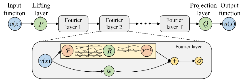
(1) The input is lifted to a higher dimensional representation by the local transformation which is commonly parameterized by a shallow fully connected neural network.
(2) The higher dimensional representation is updated iteratively by
| (7) |
Where maps to bounded linear operators on and is parameterized by , is a linear transformation, and is non-linear activation function.
(3) The output is obtained by where is the projection of and it is parameterized by a fully connected layer.Li et al. (2020a)
Denote and as Fourier transform and its inverse transform of a function respectively. By substituting the kernel integral operator in Eq. 7 with a convolution operator defined in Fourier space, the Fourier integral operator can be rewritten as Eq. 8.
| (8) |
Where is the Fourier transform of a periodic function parameterized by . The frequency mode . The finite-dimensional parameterization is obtained by truncating the Fourier series at a maximum number of modes , for . can be obtained by discretizing domain with points, where .Li et al. (2020a) By simply truncating the higher modes, can be obtained, here is the complex space. is parameterized as complex-valued-tensor containing a collection of truncated Fourier modes . Therefore, Eq. 9 can be derived by multiplying and .
| (9) |
III.2 U-net enhanced Fourier neural operator
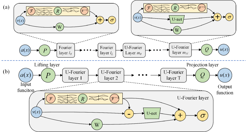
Wen et al.Wen et al. (2022) pointed out that FNO models may suffer from lower training accuracy due to the regularization impact of the FNO architecture in the multiphase flow problems.Li et al. (2020a) They introduced an improved version of the Fourier neural operator, named U-FNO, which combines the strengths of both FNO-based and CNN-based models. The detailed description of the U-FNO network architecture is given in Appendix B.
We propose a modified U-FNO architecture to better utilize the U-Net for learning small-scale flow structures, as shown in Fig. 20(b). The formulation of iterative network update is given by
| (10) |
| (11) |
Here, denotes the small-scale flow field which can be obtained by subtracting the large-scale flow field from the original flow field . Then the U-Net is used to learn the small-scale flow field. Finally, the full-field information transformed by is used to combine with FNO and U-Net, and then is connected with a nonlinear activation function to form a new U-FNO network.
Compared with the original U-FNO, our improved U-FNO performs better in 3D turbulence problems. Specifically, the minimum testing loss of original U-FNO and our modified U-FNO are 0.220 and 0.198, respectively. Therefore, the U-FNO mentioned later in this article refers to the modified U-FNO in Fig. 20(b).
III.3 The implicit Fourier neural operator
It has been demonstrated that with a large enough value of depth L, the FNO can serve as a universal approximator capable of accurately representing any continuous operator.Kovachki, Lanthaler, and Mishra (2021) However, the increase of Fourier layers brings challenge for training the network due to the vanishing of gradient problem.You et al. (2022b) To overcome the shortage mentioned above, the idea of employing the shared hidden layer has been suggested.El Ghaoui et al. (2021); Winston and Kolter (2020); Bai, Koltun, and Kolter (2020) You et al.You et al. (2022a) proposed the implicit Fourier neural operators (IFNOs) and demonstrated the technique of shallow-to-deep training. The detailed description of the IFNO network architecture is given in Appendix B.
It should be noted that the numbers of parameters of the hidden layer are independent of the layers, which distinguishes it from the FNOs. It thus can greatly reduces the total number of parameters of the model and memory-usage. Furthermore, this architecture allows for the simple implementation of the shallow-to-deep initialization method.
With increasing depth of the layer , Eq. 27 can be regarded as a discrete version of ordinary differential equations (ODEs).You et al. (2022a) Therefore, the network update can be reinterpreted as a discretization of a differential equation, and the optimal parameters obtained with layers can be served as the initial guess for deeper networks. The shallow-to-deep technique involves interpolating optimal parameters at depth and scaling them to maintain the final time of the differential equation.You et al. (2022a) This technique can effectively improve the accuracy of the network and reduce the memory cost.
IV The implicit U-Net enhanced Fourier neural operator (IU-FNO)
We introduce an implicit U-Net enhanced Fourier neural operator (IU-FNO) to integrate the advantages of U-FNO and IFNO. The architecture of IU-FNO is shown in Fig. 2. The velocity field from the first several time nodes is utilized as the input to the model, which is then converted into a high-dimensional representation via the lifting layer . Then the velocity field is iteratively updated through the implicit U-Fourier layers, and finally the output is obtained through the projection of , which is the velocity field of the next time-node. The fundamental differences between the IU-FNO and FNO models are their network structures. FNO adopts a multilayer structure, where multiple Fourier layers with independent trainable parameters are connected in series. In contrast, the IU-FNO model utilizes a single Fourier layer with shared parameters and incorporates a U-net network to capture small-scale flow structures.
The formulation of iterative implicit U-Fourier layer update can be derived as
| (12) |
| (13) |
| (14) |
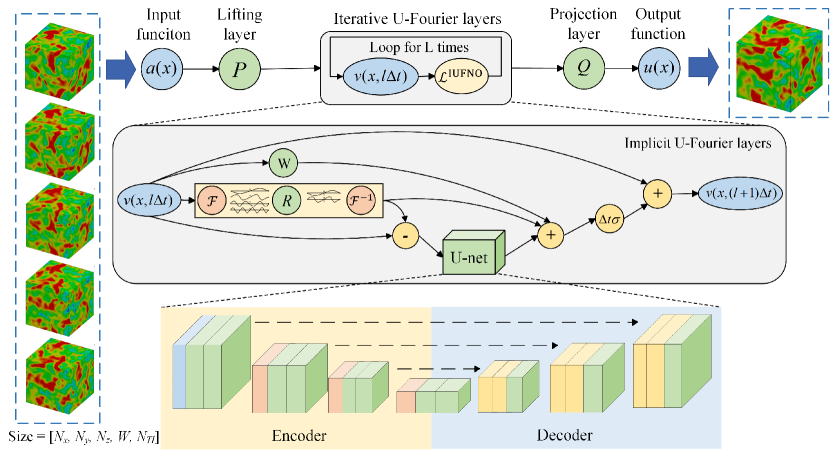
Here, has the global scale information of the flow field by combining large-scale information learned by FFT and small-scale information learned by the U-Net network . is obtained by subtracting the large-scale information from the complete field information , shown in Eq. 14. is a CNN-based network, which provides a symmetrical structure with both an encoder and a decoder. The encoder is responsible for extracting feature representations from the input data, while the decoder generates the output signals.Ronneberger, Fischer, and Brox (2015); Wang et al. (2020) Furthermore, U-Net incorporates skip connections, enabling direct transmission of feature maps from the encoder to the decoder, thereby preserving the intricate details within the fields. The U-Net architecture has a relatively small number of parameters, such that its combination with FNO has a minimal effect on the overall numbers of parameters. Additionally, the implicit utilization of a shared hidden layer has significantly reduced the number of network parameters, which can make the network very deep.
| Model | ||||
|---|---|---|---|---|
| FNO | 331.8M | 829.5M | 1659M | 3318M |
| U-FNO | 332.0M | 830.0M | 1660M | 3320M |
| IFNO | 82.97M | 82.97M | 82.97M | 82.97M |
| IU-FNO | 83.02M | 83.02M | 83.02M | 83.02M |
We compare the numbers of parameters with Fourier layer of different FNO-based models in Fourier mode equal to 20, as shown in Tab. 1. The numbers of parameters of FNO and U-FNO models are 331.8 Million and 332.0 Million, respectively, when the number of Fourier layers is set to four. However, as the number of layers increases, the size of these parameters also increases, resulting in huge computational demands that can pose significant challenges for training. By using the implicit method of sharing hidden layers, the number of network parameters of the IFNO and IU-FNO models can be independent of the number of Fourier layers . Specifically, the number of model parameters of IU-FNO is almost the same as that of IFNO. Moreover, it shows a significant reduction of approximately 75% of parameter number compared with FNO.
V Numerical Examples
In this section, the flow fields of the filtered direct numerical simulation (fDNS) of three types of turbulent flows are used for the evaluations of four FNO-based models, by comparing them against traditional LES with dynamic Smagorinsky model.Yuan et al. (2023) The instantaneous snapshots of the fDNS data are employed for initializing the LES. The three types of turbulent flows includes forced homogeneous isotropic turbulence (HIT), temporally evolving turbulent mixing layer, and decaying HIT.
In a posteriori analysis, we perform the numerical simulations with ten different random initializations for each method in forced HIT, five different initializations in temporally evolving turbulent mixing layer, and five different initializations in decaying HIT respectively. We report the average value of the statistical results of different random initializations in the posteriori analysis.
V.1 Forced homogeneous isotropic turbulence
The direct numerical simulation of forced homogeneous isotropic turbulence is performed with the uniform grid resolutions of in a cubic box of with periodic boundary conditions.Xie, Wang, and Weinan (2020); Yuan, Xie, and Wang (2020) The governing equations are spatially discretized using the pseudo-spectral method and a second-order two-step Adams-Bashforth explicit scheme is utilized for time integration.Hussaini and Zang (1987); Peyret (2002); Chen et al. (1993) The aliasing error caused by nonlinear advection terms is eliminated by truncating the high wavenumbers of Fourier modes by the two-thirds rule.Hussaini and Zang (1987) The large-scale forcing is applied by fixing the velocity spectrum within the two lowest wavenumber shells in the velocity field to maintain the turbulence in the statistically steady state.Yuan, Xie, and Wang (2020) The kinematic viscosity is adopted as , leading to the Taylor Reynolds number . To ensure that the flow has reached a statistically steady state, we save the data after a long period (more than , here is large-eddy turnover times).
The DNS data is filtered into large-scale flow fields at grid resolutions of by the sharp spectral filter (described in Section II) with cutoff wavenumber . The time step is set to 0.001 and the snapshots of the numerical solution are taken every 200 steps as a time node. 45 distinct random fields are utilized as initial conditions, with 600 time nodes being saved for each group of computations. Therefore, the fDNS data with tensor size of can be obtained and serve as a training and testing dataset.Li et al. (2022b) Specifically, the dataset we use to train the neural operator model consists of 45 groups, each group has 600 time nodes, and each time node denotes a filtered velocity field of with three directions.
Denotes the -th time-node velocity field as and the -th evolution increment filed as which is the difference of velocity field between two adjacent time nodes. The IU-FNO model takes the velocity fields of the previous five time nodes as input and produces the difference between the sixth and fifth velocity fields as output, as illustrated in Fig. 2.Li et al. (2022b) Once the predicted evolution increment is obtained from the trained model, the predicted sixth velocity field can be calculated by . In the same way, can be predicted by and so on. Therefore, 600 time-nodes in each group can generate 595 input-output pairs (), and 45 groups can produce 26775 samples where we use 80% for training and the rest of the samples for testing.Li et al. (2022b)
All four data-driven models in this study utilize the same number of the Fourier modes, specifically a value of 20, and the initial learning rate is set to .Peng et al. (2023) The Adam optimizer is used for optimization.Kingma and Ba (2014) The GELU function is chosen as the activation function.Hendrycks and Gimpel (2016) In order to ensure a fair comparison, the hyperparameters including learning rates and the decay rates are tuned for each method to minimize the training and testing loss, which is defined as
| (15) |
Here, denotes the prediction of velocity fields and is the ground truth.
| (Training Loss, Testing Loss) | ||||
|---|---|---|---|---|
| Model | ||||
| FNO | (0.225, 0.255) | N/A | N/A | N/A |
| U-FNO | (0.174, 0.198) | N/A | N/A | N/A |
| IFNO | (0.244, 0.261) | (0.216, 0.228) | (0.199, 0.214) | (0.185, 0.201) |
| IU-FNO | (0.192, 0.211) | (0.171, 0.190) | (0.140, 0.163) | (0.143, 0.155) |
A comparison of the minimum training and testing loss with Fourier layer of different FNO-based models in forced HIT is given in Tab. 2. It is shown that incorporating the U-net module to facilitate learning at small-scale information can improve the effectiveness of training and testing. Besides, the training and testing loss of the implicit method using the shared hidden layer (e.g. IFNO and IU-FNO) will be larger than FNO and U-FNO at layer . However, as the number of hidden layer loop iterations increases, a significant reduction in the loss value is observed. The smallest testing loss value is obtained when equals 40 for IU-FNO. Therefore, the number of layer with minimum loss in each model is chosen for the posteriori study. For FNO and U-FNO models, the Fourier layer number is set to 4, whereas IFNO and IU-FNO models have 40 implicit loop Fourier layers.
To avoid the over-fitting issue of the models, an additional independent ten groups of data from different initial fields are generated and utilized for the posteriori evaluation. In the a posteriori study, fDNS data is utilized as a baseline to evaluate various FNO-based models, including FNO, U-FNO, IFNO, and IU-FNO. The LES with DSM model is performed on the uniform grid with the grid resolution of in a cubic box of using the same numerical method as DNS. The LES is initialized with the instantaneous velocity field obtained from fDNS. The DMM and VGM models adopt the same initial field and computational approach as the DSM model.
V.1.1 The a posteriori study
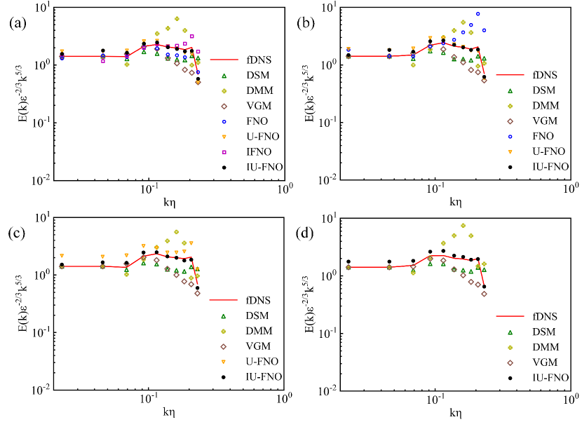
The normalized velocity spectra predicted by different FNO-based models and classical LES models at different time instants are shown in Fig. 3. Here, Kolmogorov length scale and the dissipation rate in the forced HIT are obtained from DNS data. For the traditional LES model DSM, the prediction errors become larger as the wavenumber increases. Specifically, the velocity spectrum at wavenumbers is significantly lower than fDNS results. In terms of velocity spectrum prediction, the DMM model exhibits significantly higher values than the fDNS results in the wavenumbers range of 5 to 8. In contrast, the VGM model predicts much lower results for . Overall, the normalized velocity spectrum predicted by the DSM model is more accurate than the DMM and VGM models. This study focuses on comparing the performance of FNO-based models, and we select the DSM model as the representative SGS model for comparison.
It can be seen from Fig. 3(a) that the normalized velocity spectrum predicted by data-driven models including FNO, U-FNO, and our proposed IU-FNO model are close to that of fDNS at time . Here the large-eddy turnover time is provided in Eq. (4). However, the normalized velocity spectrum is overestimated by IFNO for the high wavenumbers at time , and the prediction error becomes larger as the time increases. For the FNO and U-FNO models, large prediction errors have been identified at time and time , respectively. It is worth noting that the prediction results of the FNO, IFNO, and U-FNO models are observed to be divergent with an increase in prediction time, and lose statistical significance. Therefore, we do not present these divergent results at the later time instants. On the contrary, IU-FNO always gives accurate predictions on the velocity spectrum in both short-term and long-term predictions for . We also observe that IU-FNO is stable for (not shown here).
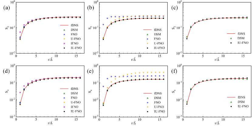
To further examine the IU-FNO model in predicting multi-scale properties of turbulence, we compute the longitudinal structure functions of the filtered velocity, which are defined by Xie et al. (2018, 2020)
| (16) |
where denotes the order of structure function and represents the longitudinal increment of the velocity at the separation . Here, is the unit vector.
Fig. 4 compares the second-order and fourth-order structure functions of the filtered velocity for different models with fDNS data at , , and . It can be seen that the DSM model overestimates the structure functions at a small distances while underestimates them at large distances compared to those of the fDNS data. Moreover, as the time increases, the deviations of the structure functions predicted by the FNO, IFNO, and U-FNO models from the fDNS data become more serious. In contrast, the IU-FNO model can always accurately predict the structure functions at both small and large separations.
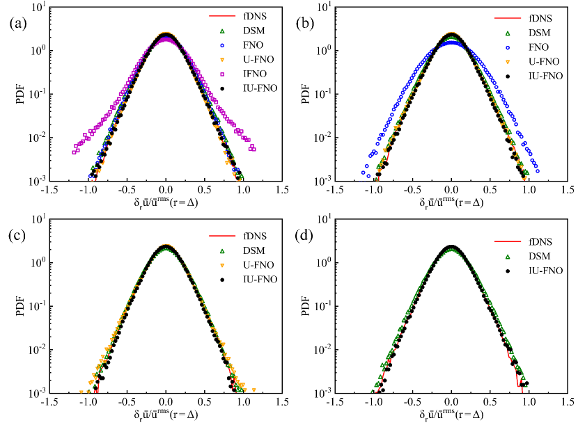
Furthermore, we compare PDFs of the normalized velocity increments with distance at different time instants in Fig. 5. It can be seen that the PDFs of the normalized velocity increments predicted by FNO, and U-FNO are in a good agreement with the fDNS data at the beginning, but the predicted PDFs become wider than the fDNS data as the time increases. The IFNO gives worst prediction on the PDF. The PDF predicted by the DSM model are also slightly wider than the fDNS results. The IU-FNO model gives the most accurate prediction on the velocity increments, demonstrating the excellent performance for both short-term and long-term predictions.
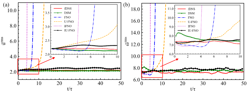
To further demonstrate the stability of different models, we display the evolution of the root-mean-square (rms) values of velocity and vorticity over time in Fig. 6. Here, we plot the results from the -th time instant. It can be seen that as the time increases gradually, the IFNO model will diverge quickly, followed by the FNO model, and the U-FNO model respectively. Since the predicted results will be used as the input for the next prediction, the prediction error will continue to be accumulated, which is one of the reasons why the data-driven model is difficult to be stable for a long-term prediction. The traditional DSM model is stable due to its dissipative characteristics.Smagorinsky (1963); Kleissl et al. (2006) Here, it is demonstrated that the proposed IU-FNO model can effectively and stably reconstrcut the long-term large-scale dynamics of the forced homogeneous isotropic turbulence.
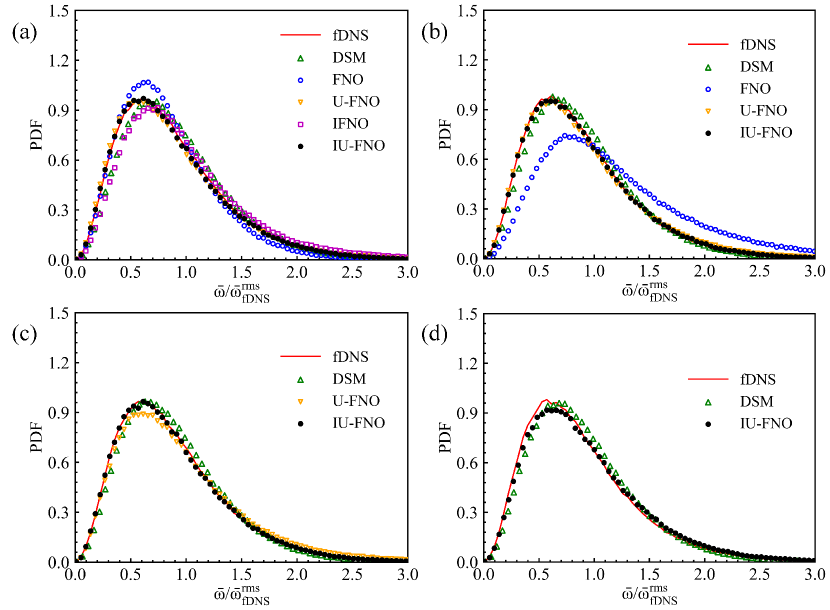
The PDFs of the normalized vorticity magnitude at different time instants are shown in Fig. 7. Here, the vorticity is normalized by the rms values of the vorticity calculated by the fDNS data. It is shown that the PDFs predicted by all FNO-based models and DSM model have a reasonable agreement with those of fDNS in the short-term prediction for . However, as the time increases, the deviation between the PDFs of predicted by FNO and U-FNO models and those of ground truth becomes more obvious. In contrast, the IU-FNO performs better than other FNO-based models in both short and long time predictions of vorticity statistics.
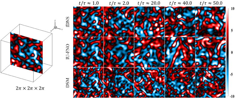
Fig. 8 illustrates the contours of the vorticity fields predicted by different models. The instantaneous snapshots are selected on the center of the y-z plane at five different time instants. The DSM model produces factitious small-scale structures of vorticity, which significantly differ from those of the fDNS data. In contrast, vorticity fields given by IU-FNO model are very close to the benchmark fDNS results in the short-term prediction and . Although the long-term prediction results of IU-FNO are not fully consistent with fDNS, its prediction of large-scale and small-scale structures is qualitatively better than that of the DSM model. Therefore, the IU-FNO model also performs better in long-term prediction of instantaneous vorticity structures, as compared to those of the DSM model.
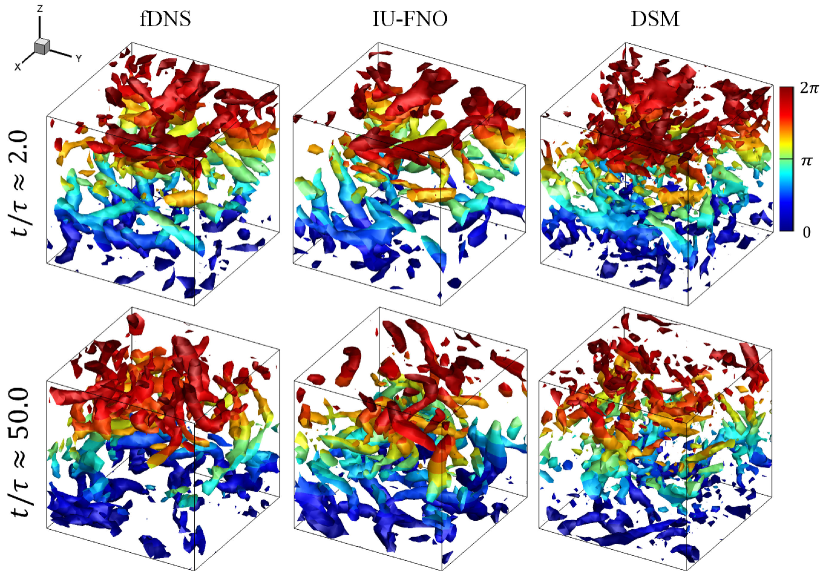
We demonstrate isosurfaces of the normalized vorticity colored by the altitude of z-direction in Fig. 9. The spatial structures predicted by DSM and IU-FNO are compared to those of the fDNS data at time and . It is revealed that the DSM model shows a limited accuracy in predicting the spatial structure of small-scale vortices. On the contrary, the IU-FNO model can better predict the overall flow structures of the vorticity field.
V.1.2 Computational efficiency
| Method | Number of parameters(Million) | GPU memory-usage(MB) | GPUs | CPUs |
|---|---|---|---|---|
| DSM | N/A | N/A | N/A | 65.31 |
| FNO | 331.8 | 3,204 | 0.058 | 2.953 |
| U-FNO | 332.0 | 3,204 | 0.076 | 3.635 |
| IFNO | 82.97 | 1,284 | 0.577 | 28.43 |
| IU-FNO | 83.02 | 1,284 | 0.783 | 32.86 |
Table. 3 compares the computational cost of 10 prediction steps, number of parameters of the model, and GPU memory-usage for different FNO-based models on predictions of forced HIT. We carry out numerical simulations by using the Pytorch. The neural network models are trained and test on Nvidia Tesla V100 GPU, where the CPU type is Intel(R) Xeon(R) Gold 6240 CPU @2.60GHz. The DSM simulations are implemented on a computing cluster, where the type of CPU is Intel Xeon Gold 6148 with 16 cores each @2.40 GHz. Moreover, we conducted supplementary tests to measure the computational time for the FNO-based models using the same CPU as the DSM model. CPUs in Table. 3 represents the time (second) required by each CPU core. Here, the FNO-based models are implemented on a single core CPU, while the DSM model is performed on CPU with 16 cores. So we assume that the CPUs of the DSM model is 16 times the actual time it takes. It can be seen that the FNO-based models are significantly more efficient than the DSM model. This is mainly attributed to the fact that the DSM model requires iterative solutions with a very small time step, while the FNO-based model can directly predict the flow state over a large time interval. In comparison to the original FNO, the IU-FNO model requires more computation time due to its deeper network. However, it is still about two times faster than the traditional DSM model. Table. 3 also indicates that the computational efficiency of the FNO-based model can be further improved remarkably by using GPU. Moreover, the parameters and the GPU memory usage of the IU-FNO network model are reduced by about 75% and 40% compared with the original FNO model respectively.
V.1.3 Generalization on higher Taylor Reynolds numbers
Here, we show that the IU-FNO model trained with low Taylor Reynolds number data can be directly used for the prediction of high Taylor Reynolds number cases without the need for additional training or modifications. The large-scale statistical features and flow structures in our simulations are observed to be insensitive to the Taylor Reynolds numbers.Li et al. (2022b) We employ five sets of HIT data with different initial fields at a Taylor Reynolds number . Owing to the large computational cost of DNS of turbulence at high Taylor Reynolds number, only 90 time nodes are computed for each initial field. Here, each time node for FNO-based model is , and the large-eddy turnover time is . For consistency, the computing devices for LES of DSM and IU-FNO are the same as those in the case of low Reynolds number. When performing the simulation for these higher Taylor Reynolds number cases on the same single CPU mentioned above, the DSM model required about 1900s to complete the task, while IU-FNO still only costs 32.26s. Thus, IU-FNO is more computationally efficient than DSM model, highlighting its considerable speed advantage. Here, DSM is performed on a higher grid resolution of to capture the small-scale fields at higher Taylor Reynolds number, but the result is still worse than the IU-FNO model.Li et al. (2022b)
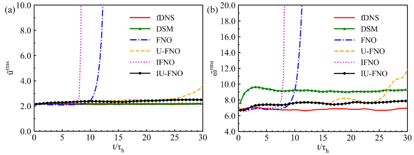
To assess the stability of the model at the high Reynolds number, we show the temporal evolutions of the rms values of velocity and vorticity in Fig. 10. It is revealed that the rms values of velocity and vorticity predicted by the IU-FNO and DSM models always perform stable, whereas other models become unstable as time increases. The rms values of velocity predicted by both the IU-FNO and DSM models show a good agreement with the fDNS data.
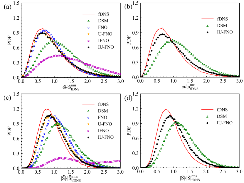
Furthermore, Fig 11(a) and (b) illustrate the PDFs of the normalized vorticity . The IU-FNO model demonstrates a higher accuracy in predicting the peak and shape of PDFs than other models. The PDFs of the normalized characteristic strain rate of forced HIT at and are displayed in Fig. 11(c) and (d), respectively. Here, the characteristic strain rate is defined by and normalized by the rms values of the corresponding fDNS data. It is shown that the IU-FNO model outperforms the DSM model by accurately recovering both the peak value and overall shape of the PDF.
V.2 Temporally evolving turbulent mixing layer
In addition to benchmarking the performance of FNO-based models and classical SGS model on 3D forced HIT, we also evaluate their capabilities on a more complex simulation task: a 3D free-shear turbulent mixing layer. We focus on the comparison between the IU-FNO model and the conventional DSM model. The turbulent mixing layer provides a suitable example for studying the effects of non-uniform turbulent shear and mixing on subgrid-scale (SGS) models.Wang et al. (2022)
The free-shear turbulent mixing layer is governed by the same Navier-Stokes equations (Eqs. 1 and 2) without the forcing term. The mixing layer is numerically simulated in a cuboid domain with lengths using a uniform grid resolution of . Here, , and denote the streamwise, normal, and spanwise directions, respectively. The initial streamwise velocity is given byWang et al. (2022); Wang, Wang, and Chen (2022); Sharan, Matheou, and Dimotakis (2019)
| (17) |
where, , is the initial momentum thickness and is the velocity difference between two equal and opposite free streams across the shear layer.Wang et al. (2022); Yuan et al. (2023) The momentum thickness quantifies the range of turbulence region in the mixing layer, which is given bySharan, Matheou, and Dimotakis (2019); Rogers and Moser (1994); Yuan et al. (2023)
| (18) |
The initial normal and spanwise velocities are given as , respectively. Here, , i.e., satisfy the Gaussian random distribution. The expectation of the distribution is and the variance of the distribution is . The Reynolds number based on the momentum thickness is defined as . Here, the kinematic viscosity of shear layer is set to , so the initial momentum thickness Reynolds number is .Yuan et al. (2023) To mitigate the impact of the top and bottom boundaries on the central mixing layer, two numerical diffusion buffer zones are implemented to the vertical edges of the computational domain.Wang, Wang, and Chen (2022); Yuan et al. (2023); Wang et al. (2022) The periodic boundary conditions in all three directions are utilized and the pseudo-spectral method with the two-thirds dealiasing rule is employed for the spatial discretization. An explicit two-step Adam-Bashforth scheme is chosen as the time-advancing scheme.
The DNS data are then explicitly filtered by the commonly-used Gaussian filter, which is defined byPope and Pope (2000); Sagaut (2006)
| (19) |
Here, the filter scale is selected for the free-shear turbulent mixing layer, where is the grid spacing of DNS. The filter-to-grid ratio FGR= is utilized and then the corresponding grid resolution of fDNS: can be obtained.Chang, Yuan, and Wang (2022); Wang et al. (2022) The LES with DSM model is performed on the uniform grid with the grid resolution of in a cuboid domain with lengths using the same numerical method as DNS and is initialized by the fDNS data.
We perform numerical simulations for 145 sets of distinct initial fields and save the results for 90 temporal snapshots for each initial field. The time interval for each snapshot is , where is the time step of DNS. Therefore, the data of size can be obtained as training and testing sets. Similar to SectionV.1, 80% of data, including 9860 input-output pairs, is used for training, and 20% of data, including 2465 pairs, is used for testing.
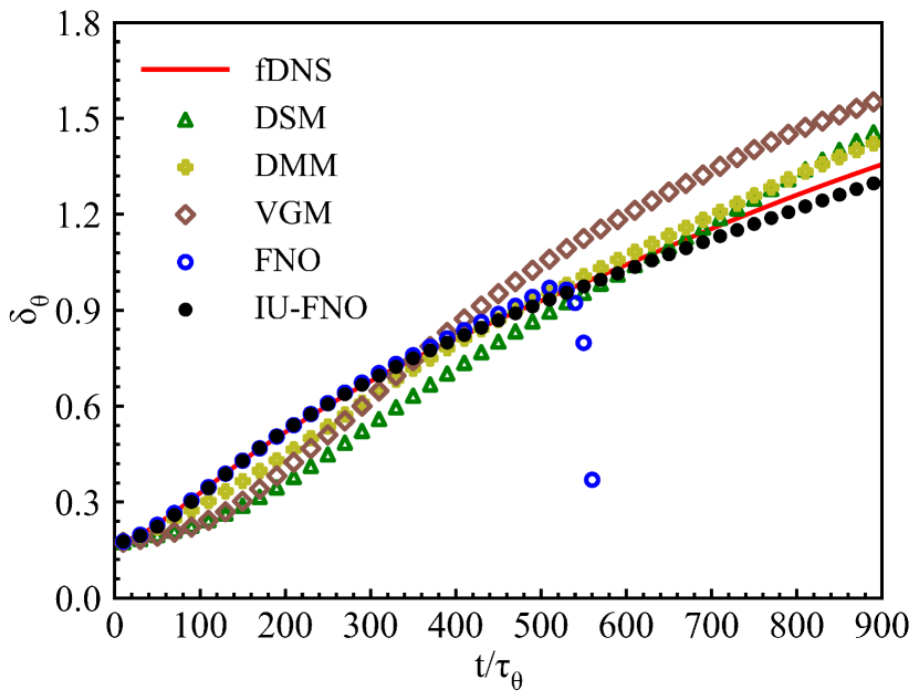
To perform a posteriori analysis, we produce additional five sets of data with different initial fields, each containing ninety time nodes. Here, ninety time nodes are equivalent to nine hundred time units normalized by . The temporal evolutions of the momentum thickness for LES using different models are shown in Fig. 12. The DSM model underestimates the momentum thickness at the beginning of the transition region while overestimates the momentum thickness in the linear growth region. In comparison to the baseline fDNS, both the DMM and VGM models exhibit lower predicted values at the beginning, which gradually increase and eventually exceed the actual fDNS results. Since the three classical LES models exhibit similar performance, we select the DSM model for comparison with the FNO-based models. The FNO model shows a good ability to capture the momentum thickness growth rate during the early stages of temporal development. However, its prediction becomes invalid after 500 time units . In contrast, the predictions of the IU-FNO model always show a good agreement with fDNS in both transition and linear growth regions.
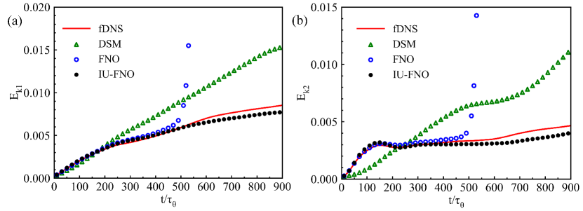
Furthermore, the temporal evolutions of the streamwise turbulent kinetic energy and normal turbulent kinetic energy are displayed in Fig. 13. Here, denotes a spatial average over the whole computational domain. The turbulent kinetic energy in various directions increases gradually during the shear layer development in fDNS. Both streamwise and normal kinetic energy predicted by the DSM model are much larger than those of fDNS. FNO predicts reasonable results during the first 450 time units , after that the results diverge quickly. By contrast, the IU-FNO model can well predict the kinetic energy in both streamwise and normal directions during the whole development of the shear layer, which is the closest to the fDNS data.
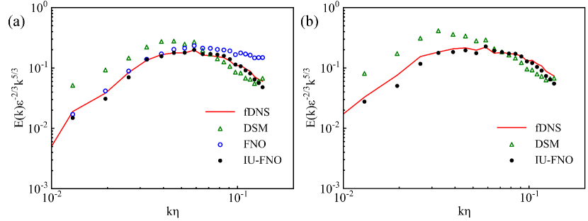
We then compare the normalized velocity spectrum of different models at time instants and , as shown in Fig. 14. Here, Kolmogorov length scale at both and . The dissipation rate at , and at in the free-shear turbluent mixing layer. It can be seen that the normalized velocity spectrum predicted by the DSM model is overestimated at low wavenumbers and is underestimated at high wavenumbers when compared to those of the fDNS. The normalized velocity spectrum predicted by FNO is higher than benchmark fDNS at high wavenumbers, and the deviation will be larger as the time increases. In comparison, the IU-FNO model can accurately predict energy spectrum that agrees well with the fDNS data at various time instants.
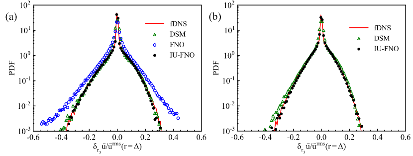
Figure. 15 illustrates the PDFs of velocity increment in the spanwise direction. Here, the spanwise velocity increment is given by , where denotes the unit vector in the spanwise direction and the velocity increments are normalized by the rms values of velocity . The sharp peak of PDF is due to the non-turbulent regions where the velocity increment is nearly zero in the spanwise direction.Wang et al. (2022) The regions with non-zero velocity increments are predominantly governed by turbulence. It is shown that the IU-FNO model demonstrates better performance compared to both FNO and DSM models at different time instants.
Finally, we compare the vortex structures predicted by the DSM model and IU-FNO model with fDNS data. The Q-criterion has been widely used for visualizing vortex structures in turbulent flows and is defined byHunt, Wray, and Moin (1988); Dubief and Delcayre (2000); Zhan et al. (2019)
| (20) |
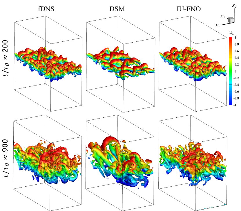
where is the filtered rotation-rate tensor. Fig. 16 displays the instantaneous isosurfaces of at and colored by the streamwise velocity. It is observed that the DSM model predicts relatively larger vortex structures compared to the fDNS result. On the contrary, the IU-FNO model demonstrates a closer agreement with fDNS results especially in terms of reconstructing the small vortex structures, highlighting its advantage in improving the accuracy of LES.
V.3 Decaying homogeneous isotropic turbulence
We assess the extrapolation ability of different FNO-based models in LES of the decaying homogeneous isotropic turbulence (HIT). The numerical simulation of decaying HIT is conducted in a cubic box of with periodic boundary conditions, and the numerical method is consistent with the forced HIT. The governing equations are spatially discretized using the pseudo-spectral method, incorporating the two-thirds dealiasing rule, at a uniform grid resolution of . The temporal discretization scheme employs the explicit second-order two-step Adams-Bashforth method. We use the statistically steady flow field of the forced HIT as the initial field for the simulation of decaying turbulence. DNS of decaying turbulence is performed over about six large-eddy turnover times. In order to assess the extrapolation ability of different FNO-based models, only the flow fields at first two large-eddy turnover times are used for training, and the flow fields at are in the unseen flow regime where the magnitude of velocity fluctuation is different from the training data.
The kinematic viscosity is set to and the initial Taylor Reynolds number is . The sharp spectral filter(mentioned in Section II) with cutoff wavenumber is used to filter the DNS data. Here, we calculated 595 different sets of initial fields and stored a snapshot every . Finally, the fDNS data of size can be obtained, and 80% of datas are used for training and 20% for testing.

After training, five more groups of data with different initial fields are generated to perform a posteriori analysis. Figure. 17 compares the temporal evolutions of the turbulent kinetic energy and the resolved dissipation rate of DSM, FNO, and IU-FNO models with fDNS data. Here, the dissipation rate is defined by . It can be seen that the kinetic energy gradually decays from the initial state over time, and all models can predict the turbulent kinetic energy well in the short period. However, the dissipation rate predicted by IU-FNO is more accurate than those of the DSM and FNO models at .
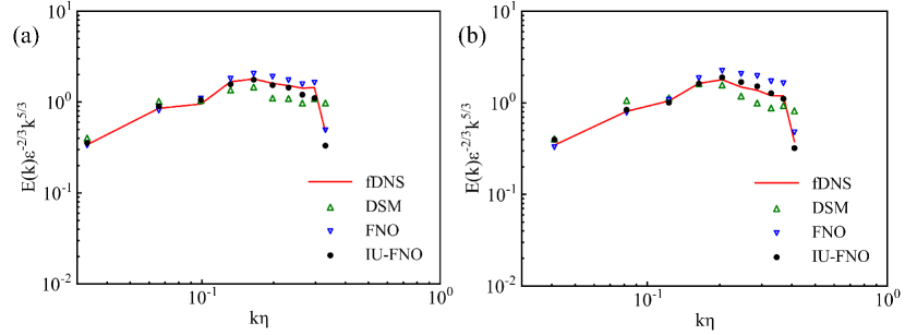
Further, we evaluate the normalized velocity spectra for different models at two different time instants and in Fig. 18. Here, Kolmogorov length scale at , and at . The dissipation rate at , and at in the decaying HIT. The kinetic energy at all wavenumbers decreases with the time. The DSM model overestimates the kinetic energy at low wavenumbers. The FNO model overpredicts the energy spectrum at all wavenumbers. In contrast, the normalized velocity spectrum predicted by the IU-FNO model is in a good agreement with fDNS data.
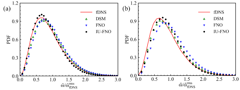
Finally, the PDFs of the normalized vorticity at the dimensionless time and are depicted in Fig. 19. The rms values of the vorticity calculated by the fDNS data are used for normalization. Both the DSM model and FNO model give the wrong prediction of the peak location. On the contrary, the IU-FNO model slightly outperforms these models at both and , which provides a reasonably accurate prediction for both the locations and peaks of the PDFs of the vorticity.
VI Discussion and future work
Simulations of three-dimensional (3D) nonlinear partial differential equations (PDEs) are of great importance in engineering applications. While data-driven approaches have been widely successful in solving one-dimensional (1D) and two-dimensional (2D) PDEs, the relevant works on data-driven fast simulations of 3D PDFs are relatively rare. The need for significant model complexity and a large number of parameters to accurately model the non-linear interactions in 3D PDEs (including turbulent flows) is a major challenge. In such situations, training and implementing neural networks may not be as efficient as traditional numerical methods.
Recently, the FNO has proven to be a highly effective surrogate model in solving PDEs, indicating its significant potential for addressing 3D nonlinear problems.Li et al. (2020a, 2022a); De Hoop et al. (2022) The utilization of FNO in 3D turbulence has attracted more and more attention. Li et al. utilized FNO for LES of 3D forced HIT and achieved faster and more accurate prediction compared to the classical LES with the dynamic Smagorinsky model and dynamic mixed model.Li et al. (2022b) Peng et al. proposed a linear attention coupled Fourier neural operator (LAFNO) to further improve the model accuracy in simulating 3D forced HIT, and free-shear turbulence.Peng et al. (2023) However, model errors will accumulate over time, leading a challenge for maintaining high accuracy in long-term predictions. In addition, the memory size imposes a limitation on number of layers in the original form of FNO.
In this work, we investigate the effectiveness of implicit layer that utilize shared Fourier layers, which can enable the neural network to be expanded to greater depths, thereby enhancing its capability to approximate complex functions. Simultaneously, we incorporate the U-net network to complement small-scale information, which further enhances the stability of the model. The results demonstrate that the proposed IU-FNO model outperforms the original FNO model in terms of accuracy and stability in predicting 3D turbulent flows, including forced homogeneous isotropic turbulence, free-shear turbulent mixing layer, and decaying homogeneous isotropic turbulence. Moreover, IU-FNO demonstrates long-term stable predictions, which has not been achieved by previous versions of FNO. In comparison with the original FNO, IU-FNO reduces the network parameters by approximately 75%, and the number of parameters is independent of the number of network layers. Meanwhile, the IU-FNO model also demonstrates improved generalizability to higher Reynolds numbers, and can predict unseen flow regime in decaying turbulence. Therefore, the IU-FNO approach serves as a valuable guide for modeling large-scale dynamics of more complex turbulence. Since we are using a purely data-driven approach without explicitly embedding any physical knowledge, the predicted results might not strictly satisfy the N-S equations. However, the IU-FNO model is capable of approximating the N-S equations from data.
One limitation of the proposed model is that it has only been tested on simple flows, whereas the flows in engineering applications are often much more complex. While the IU-FNO model is effective in predicting flow types under uniform grid and periodic boundary conditions, it requires further improvement to be applicable to non-uniform grid and non-periodic boundary conditions. Another disadvantage of the proposed model is its high dependence on data. As a purely data-driven model, it requires a substantial amount of data for training. Recently, more sophisticated improvements of the FNO framework have been proposed to simulate complex flows, including the adaptive Fourier neural operators (AFNO)Guibas et al. (2021); Kurth et al. (2022) and physics-informed neural operator (PINO).Li et al. (2021b); Rosofsky and Huerta (2023) Li et al. introduced geo-FNO, a method that can handle PDEs on irregular geometries by mapping the input physical domain into a uniform latent space using a deformation function. The FNO model with the FFT is then applied in the latent space to solve the PDEs.Li et al. (2022a) The ability to handle arbitrary geometries is essential for solving engineering flows, which often involve complex geometries with irregular boundaries. Most of advanced FNO variants have been only tested in 2D problems, whereas most flows in engineering applications are 3D. In future work, the geo-FNO can be extended and integrated with the proposed IU-FNO models for fast simulations of 3D complex turbulence.
VII Concludsion
In this work, we proposed an implicit U-Net enhanced Fourier neural operator (IU-FNO) model to predict long-term large-scale dynamics of three-dimensional turbulence. The IU-FNO is verified in the large-eddy simulations of three types of 3D turbulence, including forced homogeneous isotropic turbulence, free-shear turbulent mixing layer, and decaying homogeneous isotropic turbulence.
Numerical simulations demonstrate that: 1) The IU-FNO model performs a superior capability to reconstruct a variety of statistics of velocity and vorticity fields, and the instantaneous spatial structures of vorticity, compared to other FNO-based models and classical DSM model. 2)The IU-FNO model has the capability of accurate predictions for long-time dynamics of 3D turbulence, which can not be achieved by previous forms of FNO. 3) IU-FNO model employs implicit loop Fourier layers to reduce the number of network parameters by approximately 75% compared to the original FNO. 4)The IU-FNO model is much more efficient than traditional LES with DSM model, and shows an enhanced capacity for generalization to high Reynolds numbers, and can make predictions on unseen flow regime of decaying turbulence. Therefore, the proposed IU-FNO approach has the great potential in developing advanced neural network models to solve 3D nonlinear problems in engineering applications.
Acknowledgements.
This work was supported by the National Natural Science Foundation of China (NSFC Grant Nos. 91952104, 92052301, 12172161 and 91752201), by the NSFC Basic Science Center Program (grant no. 11988102), by the Shenzhen Science and Technology Program (Grants No.KQTD20180411143441009), by Key Special Project for Introduced Talents Team of Southern Marine Science and Engineering Guangdong Laboratory (Guangzhou) (Grant No. GML2019ZD0103), and by Department of Science and Technology of Guangdong Province (No.2020B1212030001). This work was also supported by Center for Computational Science and Engineering of Southern University of Science and Technology.AUTHOR DECLARATIONS
Conflict of Interest
The authors have no conflicts to disclose.
Data Availability
The data that support the findings of this study are available from the corresponding author upon reasonable request.
Appendix A Conventional subgrid-scale model for LES
In this appendix, we mainly introduce three classical LES models, including dynamic Smagorinsky model (DSM), velocity gradient model (VGM) and dynamic mixed model (DMM). One of the most widely used functional models is the Smagorinsky model, given bySmagorinsky (1963); Lilly (1967); Germano (1992)
| (21) |
where represents the strain rate of the filtered velocity, and stands for the characteristic filtered strain rate. is the Kronecker delta operator, and denotes the filter width.
The coefficient can be obtained either through theoretical analysis or empirical calibration.Lilly (1967) The widely adopted strategy involves implementing the least-squares dynamic methodology by utilizing the Germano identity, resulting in the dynamic Smagorinsky model (DSM) with the coefficient given byGermano et al. (1991); Lilly (1992)
| (22) |
Here, the Leonard stress , and with and . Specially, an overbar denotes the filtering at scale , a tilde represents the test filtering operation at the double-filtering scale .
A representative structural model is the velocity gradient model (VGM) based on the truncated Taylor series expansions, given byClark, Ferziger, and Reynolds (1979)
| (23) |
The dynamic mixed model (DMM) combines the scale-similarity model with the dissipative Smagorinsky term, and is given byLiu, Meneveau, and Katz (1994); Shi, Xiao, and Chen (2008)
| (24) |
Here, an overbar denotes the filtering at scale , and a tilde represents the test filtering operation at the double-filtering scale . The spectral filter is employed to double-filtering in HIT, and a Gaussian filter is utilized in free-shear turbluent mixing layer. Similar to the DSM model, the model coefficients and of the DMM model are dynamically determined using the Germano identity through the least-squares algorithm. and are expressed asYuan, Xie, and Wang (2020); Xie, Yuan, and Wang (2020)
| (25) |
| (26) |
where , and . Here, , , , and The hat denotes the filter at scale .
Appendix B The Details of related Fourier neural operator methods
In this appendix, we introduce the details of related Fourier neural operators, including U-FNO and IFNO.
Fig. 20(a) illustrates the architectures of the U-FNO model. The U-FNO employ iterative architectures: where for and for are sequences of functions taking values in .Wen et al. (2022) Therefore, when doing local transformation projection, the operation is performed on . Specifically, denotes -th Fourier layer which is the same as original FNO architecture. represents -th U-Fourier layer which is given as
| (27) |
Here, , , and have the same meaning as defined in Section III.1. denotes a U-Net CNN operator. The architecture of U-FNO differs from the original Fourier layer in FNO by incorporating a U-Net path into each U-Fourier layer. The purpose of the U-Net is to perform local convolutions that enhance the representation capability of the U-FNO, particularly for small-scale flow structures.
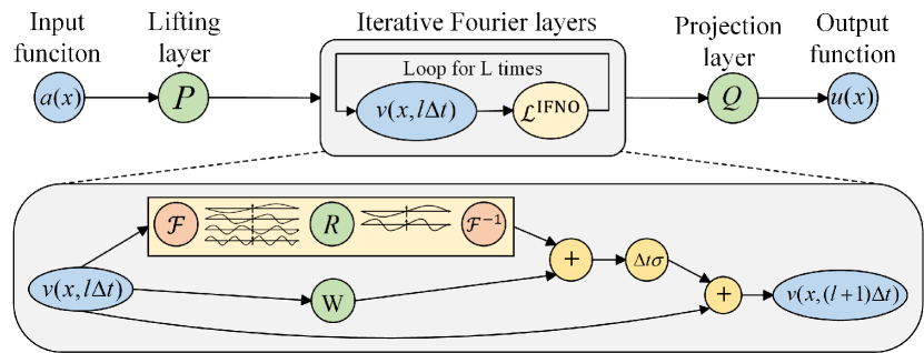
The architecture of IFNO is shown in Fig. 21, which can greatly reduce the number of trainable parameters and memory cost, and overcome the vanishing gradient problem of training networks with deep layers. The iterative network update of IFNO is given asYou et al. (2022a)
| (28) | ||||
The IFNO model employs a parameter-sharing strategy and continuously optimizes the network parameters through iterative loops to enhance its accuracy. This approach is effective in improving the performance of the network and enables it to handle complex data and nonlinear problems more efficiently.
References
- Brunton, Noack, and Koumoutsakos (2020) S. L. Brunton, B. R. Noack, and P. Koumoutsakos, “Machine learning for fluid mechanics,” Annu. Rev. Fluid Mech. 52, 477–508 (2020).
- Duraisamy, Iaccarino, and Xiao (2019) K. Duraisamy, G. Iaccarino, and H. Xiao, “Turbulence modeling in the age of data,” Annu. Rev. Fluid Mech. 51, 357–377 (2019).
- Liu et al. (2020) B. Liu, J. Tang, H. Huang, and X.-Y. Lu, “Deep learning methods for super-resolution reconstruction of turbulent flows,” Phys. Fluids 32, 025105 (2020).
- Vignon, Rabault, and Vinuesa (2023) C. Vignon, J. Rabault, and R. Vinuesa, “Recent advances in applying deep reinforcement learning for flow control: Perspectives and future directions,” Phys. Fluids 35 (2023).
- Zuo et al. (2023) K. Zuo, Z. Ye, W. Zhang, X. Yuan, and L. Zhu, “Fast aerodynamics prediction of laminar airfoils based on deep attention network,” Phys. Fluids 35 (2023).
- Maulik et al. (2018) R. Maulik, O. San, A. Rasheed, and P. Vedula, “Data-driven deconvolution for large eddy simulations of Kraichnan turbulence,” Phys. Fluids 30, 125109 (2018).
- Yuan et al. (2021) Z. Yuan, Y. Wang, C. Xie, and J. Wang, “Dynamic iterative approximate deconvolution models for large-eddy simulation of turbulence,” Phys. Fluids 33, 085125 (2021).
- Wang et al. (2021) Y. Wang, Z. Yuan, C. Xie, and J. Wang, “Artificial neural network-based spatial gradient models for large-eddy simulation of turbulence,” AIP Adv. 11, 055216 (2021).
- Beck, Flad, and Munz (2018) A. D. Beck, D. G. Flad, and C.-D. Munz, “Deep neural networks for data-driven turbulence models,” arXiv preprint arXiv:1806.04482 (2018).
- Xie et al. (2019) C. Xie, J. Wang, K. Li, and C. Ma, “Artificial neural network approach to large-eddy simulation of compressible isotropic turbulence,” Phys. Rev. E 99, 053113 (2019).
- Wang et al. (2018) Z. Wang, K. Luo, D. Li, J. Tan, and J. Fan, “Investigations of data-driven closure for subgrid-scale stress in large-eddy simulation,” Phys. Fluids 30, 125101 (2018).
- Sarghini, De Felice, and Santini (2003) F. Sarghini, G. De Felice, and S. Santini, “Neural networks based subgrid scale modeling in large eddy simulations,” Comput Fluids 32, 97–108 (2003).
- Gamahara and Hattori (2017) M. Gamahara and Y. Hattori, “Searching for turbulence models by artificial neural network,” Phys. Rev. Fluid 2, 054604 (2017).
- Zhou et al. (2019) Z. Zhou, G. He, S. Wang, and G. Jin, “Subgrid-scale model for large-eddy simulation of isotropic turbulent flows using an artificial neural network,” Comput Fluids 195, 104319 (2019).
- Li et al. (2021a) H. Li, Y. Zhao, J. Wang, and R. D. Sandberg, “Data-driven model development for large-eddy simulation of turbulence using gene-expression programing,” Phys. Fluids 33, 125127 (2021a).
- Guan et al. (2022) Y. Guan, A. Chattopadhyay, A. Subel, and P. Hassanzadeh, “Stable a posteriori LES of 2D turbulence using convolutional neural networks: Backscattering analysis and generalization to higher Re via transfer learning,” J. Comput. Phys. 458, 111090 (2022).
- Ling, Kurzawski, and Templeton (2016) J. Ling, A. Kurzawski, and J. Templeton, “Reynolds averaged turbulence modelling using deep neural networks with embedded invariance,” J. Fluid Mech. 807, 155–166 (2016).
- Tabe Jamaat and Hattori (2023) G. Tabe Jamaat and Y. Hattori, “A priori assessment of nonlocal data-driven wall modeling in large eddy simulation,” Phys. Fluids 35 (2023).
- Beck, Flad, and Munz (2019) A. Beck, D. Flad, and C.-D. Munz, “Deep neural networks for data-driven LES closure models,” J. Comput. Phys. 398, 108910 (2019).
- Park and Choi (2021) J. Park and H. Choi, “Toward neural-network-based large eddy simulation: Application to turbulent channel flow,” J. Fluid Mech. 914, A16 (2021).
- Yang et al. (2019) X. Yang, S. Zafar, J.-X. Wang, and H. Xiao, “Predictive large-eddy-simulation wall modeling via physics-informed neural networks,” Phys. Rev. Fluid 4, 034602 (2019).
- LeCun, Bengio, and Hinton (2015) Y. LeCun, Y. Bengio, and G. Hinton, “Deep learning,” nature 521, 436–444 (2015).
- Lusch, Kutz, and Brunton (2018) B. Lusch, J. N. Kutz, and S. L. Brunton, “Deep learning for universal linear embeddings of nonlinear dynamics,” Nat. Commun. 9, 4950 (2018).
- Sirignano and Spiliopoulos (2018) J. Sirignano and K. Spiliopoulos, “DGM: A deep learning algorithm for solving partial differential equations,” J. Comput. Phys. 375, 1339–1364 (2018).
- Tang et al. (2021) H. Tang, L. Li, M. Grossberg, Y. Liu, Y. Jia, S. Li, and W. Dong, “An exploratory study on machine learning to couple numerical solutions of partial differential equations,” Commun Nonlinear Sci Numer Simul 97, 105729 (2021).
- Kovachki et al. (2023) N. Kovachki, Z. Li, B. Liu, K. Azizzadenesheli, K. Bhattacharya, A. Stuart, and A. Anandkumar, “Neural Operator: Learning Maps Between Function Spaces With Applications to PDEs,” J Mach Learn Res 24, 1–97 (2023).
- Goswami et al. (2022) S. Goswami, K. Kontolati, M. D. Shields, and G. E. Karniadakis, “Deep transfer learning for partial differential equations under conditional shift with DeepONet,” arXiv preprint arXiv:2204.09810 (2022).
- Cai et al. (2021) S. Cai, Z. Mao, Z. Wang, M. Yin, and G. E. Karniadakis, “Physics-informed neural networks (PINNs) for fluid mechanics: A review,” Acta Mech Sin 37, 1727–1738 (2021).
- Wang et al. (2020) R. Wang, K. Kashinath, M. Mustafa, A. Albert, and R. Yu, “Towards physics-informed deep learning for turbulent flow prediction,” in Proceedings of the 26th ACM SIGKDD International Conference on Knowledge Discovery & Data Mining (2020) pp. 1457–1466.
- Lanthaler, Mishra, and Karniadakis (2022) S. Lanthaler, S. Mishra, and G. E. Karniadakis, “Error estimates for deeponets: A deep learning framework in infinite dimensions,” Transactions of Mathematics and Its Applications 6, tnac001 (2022).
- Karniadakis et al. (2021) G. E. Karniadakis, I. G. Kevrekidis, L. Lu, P. Perdikaris, S. Wang, and L. Yang, “Physics-informed machine learning,” Nat. Rev. Phys. 3, 422–440 (2021).
- Raissi, Perdikaris, and Karniadakis (2017) M. Raissi, P. Perdikaris, and G. E. Karniadakis, “Physics informed deep learning (part i): Data-driven solutions of nonlinear partial differential equations,” arXiv preprint arXiv:1711.10561 (2017).
- Raissi, Perdikaris, and Karniadakis (2019) M. Raissi, P. Perdikaris, and G. E. Karniadakis, “Physics-informed neural networks: A deep learning framework for solving forward and inverse problems involving nonlinear partial differential equations,” J. Comput. Phys. 378, 686–707 (2019).
- Xu, Zhang, and Wang (2021) H. Xu, W. Zhang, and Y. Wang, “Explore missing flow dynamics by physics-informed deep learning: The parameterized governing systems,” Phys. Fluids 33, 095116 (2021).
- Chen et al. (2021) Y. Chen, D. Huang, D. Zhang, J. Zeng, N. Wang, H. Zhang, and J. Yan, “Theory-guided hard constraint projection (HCP): A knowledge-based data-driven scientific machine learning method,” J. Comput. Phys. 445, 110624 (2021).
- Jin et al. (2021) X. Jin, S. Cai, H. Li, and G. E. Karniadakis, “NSFnets (Navier-Stokes flow nets): Physics-informed neural networks for the incompressible Navier-Stokes equations,” J. Comput. Phys. 426, 109951 (2021).
- Wu and Xiu (2020) K. Wu and D. Xiu, “Data-driven deep learning of partial differential equations in modal space,” J. Comput. Phys. 408, 109307 (2020).
- Xu, Zhang, and Zeng (2021) H. Xu, D. Zhang, and J. Zeng, “Deep-learning of parametric partial differential equations from sparse and noisy data,” Phys. Fluids 33, 037132 (2021).
- Lu et al. (2022) L. Lu, X. Meng, S. Cai, Z. Mao, S. Goswami, Z. Zhang, and G. E. Karniadakis, “A comprehensive and fair comparison of two neural operators (with practical extensions) based on fair data,” Comput Methods Appl Mech Eng 393, 114778 (2022).
- Oommen et al. (2022) V. Oommen, K. Shukla, S. Goswami, R. Dingreville, and G. E. Karniadakis, “Learning two-phase microstructure evolution using neural operators and autoencoder architectures,” NPJ Comput. Mater. 8, 190 (2022).
- Li et al. (2020a) Z. Li, N. Kovachki, K. Azizzadenesheli, B. Liu, K. Bhattacharya, A. Stuart, and A. Anandkumar, “Fourier neural operator for parametric partial differential equations,” arXiv preprint arXiv:2010.08895 (2020a).
- Chen, Viquerat, and Hachem (2019) J. Chen, J. Viquerat, and E. Hachem, “U-net architectures for fast prediction of incompressible laminar flows,” arXiv preprint arXiv:1910.13532 (2019).
- He et al. (2016) K. He, X. Zhang, S. Ren, and J. Sun, “Deep residual learning for image recognition,” in Proceedings of the IEEE conference on computer vision and pattern recognition (2016) pp. 770–778.
- Peng, Yuan, and Wang (2022) W. Peng, Z. Yuan, and J. Wang, “Attention-enhanced neural network models for turbulence simulation,” Phys. Fluids 34, 025111 (2022).
- Wen et al. (2022) G. Wen, Z. Li, K. Azizzadenesheli, A. Anandkumar, and S. M. Benson, “U-FNO—An enhanced Fourier neural operator-based deep-learning model for multiphase flow,” Adv Water Resour 163, 104180 (2022).
- You et al. (2022a) H. You, Q. Zhang, C. J. Ross, C.-H. Lee, and Y. Yu, “Learning deep implicit Fourier neural operators (IFNOs) with applications to heterogeneous material modeling,” Comput Methods Appl Mech Eng 398, 115296 (2022a).
- Li et al. (2022a) Z. Li, D. Z. Huang, B. Liu, and A. Anandkumar, “Fourier neural operator with learned deformations for pdes on general geometries,” arXiv preprint arXiv:2207.05209 (2022a).
- Jiang et al. (2023) Z. Jiang, M. Zhu, D. Li, Q. Li, Y. O. Yuan, and L. Lu, “Fourier-MIONet: Fourier-enhanced multiple-input neural operators for multiphase modeling of geological carbon sequestration,” arXiv preprint arXiv:2303.04778 (2023).
- Tran et al. (2021) A. Tran, A. Mathews, L. Xie, and C. S. Ong, “Factorized Fourier neural operators,” arXiv preprint arXiv:2111.13802 (2021).
- Renn et al. (2023) P. I. Renn, C. Wang, S. Lale, Z. Li, A. Anandkumar, and M. Gharib, “Forecasting subcritical cylinder wakes with Fourier Neural Operators,” arXiv preprint arXiv:2301.08290 (2023).
- Li et al. (2021b) Z. Li, H. Zheng, N. Kovachki, D. Jin, H. Chen, B. Liu, K. Azizzadenesheli, and A. Anandkumar, “Physics-informed neural operator for learning partial differential equations,” arXiv preprint arXiv:2111.03794 (2021b).
- Guibas et al. (2021) J. Guibas, M. Mardani, Z. Li, A. Tao, A. Anandkumar, and B. Catanzaro, “Adaptive Fourier neural operators: Efficient token mixers for transformers,” arXiv preprint arXiv:2111.13587 (2021).
- Hao et al. (2023) Z. Hao, C. Ying, Z. Wang, H. Su, Y. Dong, S. Liu, Z. Cheng, J. Zhu, and J. Song, “GNOT: A General Neural Operator Transformer for Operator Learning,” arXiv preprint arXiv:2302.14376 (2023).
- Benitez et al. (2023) J. A. L. Benitez, T. Furuya, F. Faucher, X. Tricoche, and M. V. de Hoop, “Fine-tuning Neural-Operator architectures for training and generalization,” arXiv preprint arXiv:2301.11509 (2023).
- Choubineh et al. (2023) A. Choubineh, J. Chen, D. A. Wood, F. Coenen, and F. Ma, “Fourier Neural Operator for Fluid Flow in Small-Shape 2D Simulated Porous Media Dataset,” Algorithms 16, 24 (2023).
- Momenifar et al. (2022) M. Momenifar, E. Diao, V. Tarokh, and A. D. Bragg, “Dimension reduced turbulent flow data from deep vector quantisers,” J. Turbul. 23, 232–264 (2022).
- Mohan et al. (2020) A. T. Mohan, D. Tretiak, M. Chertkov, and D. Livescu, “Spatio-temporal deep learning models of 3D turbulence with physics informed diagnostics,” J. Turbul. 21, 484–524 (2020).
- Ren et al. (2021) J. Ren, H. Wang, G. Chen, K. Luo, and J. Fan, “Predictive models for flame evolution using machine learning: A priori assessment in turbulent flames without and with mean shear,” Phys. Fluids 33, 055113 (2021).
- Nakamura et al. (2021) T. Nakamura, K. Fukami, K. Hasegawa, Y. Nabae, and K. Fukagata, “Convolutional neural network and long short-term memory based reduced order surrogate for minimal turbulent channel flow,” Phys. Fluids 33, 025116 (2021).
- Lehmann et al. (2023) F. Lehmann, F. Gatti, M. Bertin, and D. Clouteau, “Fourier Neural Operator Surrogate Model to Predict 3D Seismic Waves Propagation,” arXiv preprint arXiv:2304.10242 (2023).
- Li et al. (2022b) Z. Li, W. Peng, Z. Yuan, and J. Wang, “Fourier neural operator approach to large eddy simulation of three-dimensional turbulence,” Theor. App. Mech. Lett. 12, 100389 (2022b).
- Peng et al. (2023) W. Peng, Z. Yuan, Z. Li, and J. Wang, “Linear attention coupled Fourier neural operator for simulation of three-dimensional turbulence,” Phys. Fluids 35, 015106 (2023).
- Pope and Pope (2000) S. B. Pope and S. B. Pope, Turbulent flows (Cambridge university press, 2000).
- Ishihara, Gotoh, and Kaneda (2009) T. Ishihara, T. Gotoh, and Y. Kaneda, “Study of high–Reynolds number isotropic turbulence by direct numerical simulation,” Annu. Rev. Fluid Mech. 41, 165–180 (2009).
- Wang et al. (2022) Y. Wang, Z. Yuan, X. Wang, and J. Wang, “Constant-coefficient spatial gradient models for the sub-grid scale closure in large-eddy simulation of turbulence,” Phys. Fluids 34, 095108 (2022).
- Lesieur and Metais (1996) M. Lesieur and O. Metais, “New trends in large-eddy simulations of turbulence,” Annu. Rev. Fluid Mech. 28, 45–82 (1996).
- Meneveau and Katz (2000) C. Meneveau and J. Katz, “Scale-invariance and turbulence models for large-eddy simulation,” Annu. Rev. Fluid Mech. 32, 1–32 (2000).
- Sagaut (2006) P. Sagaut, Large eddy simulation for incompressible flows: an introduction (Springer Science & Business Media, 2006).
- Chang, Yuan, and Wang (2022) N. Chang, Z. Yuan, and J. Wang, “The effect of sub-filter scale dynamics in large eddy simulation of turbulence,” Phys. Fluids 34, 095104 (2022).
- Moser, Haering, and Yalla (2021) R. D. Moser, S. W. Haering, and G. R. Yalla, “Statistical properties of subgrid-scale turbulence models,” Annu. Rev. Fluid Mech. 53, 255–286 (2021).
- Johnson (2022) P. L. Johnson, “A physics-inspired alternative to spatial filtering for large-eddy simulations of turbulent flows,” J. Fluid Mech. 934, A30 (2022).
- Rashid et al. (2022) M. M. Rashid, T. Pittie, S. Chakraborty, and N. A. Krishnan, “Learning the stress-strain fields in digital composites using Fourier neural operator,” Iscience 25, 105452 (2022).
- Pathak et al. (2022) J. Pathak, S. Subramanian, P. Harrington, S. Raja, A. Chattopadhyay, M. Mardani, T. Kurth, D. Hall, Z. Li, K. Azizzadenesheli, et al., “Fourcastnet: A global data-driven high-resolution weather model using adaptive Fourier neural operators,” arXiv preprint arXiv:2202.11214 (2022).
- Beauzamy (2011) B. Beauzamy, Introduction to Banach spaces and their geometry (Elsevier, 2011).
- Vapnik (1999) V. N. Vapnik, “An overview of statistical learning theory,” IEEE Trans Neural Netw 10, 988–999 (1999).
- Li et al. (2020b) Z. Li, N. Kovachki, K. Azizzadenesheli, B. Liu, K. Bhattacharya, A. Stuart, and A. Anandkumar, “Neural operator: Graph kernel network for partial differential equations,” arXiv preprint arXiv:2003.03485 (2020b).
- Kovachki, Lanthaler, and Mishra (2021) N. Kovachki, S. Lanthaler, and S. Mishra, “On universal approximation and error bounds for Fourier neural operators,” J Mach Learn Res 22, 13237–13312 (2021).
- You et al. (2022b) H. You, Y. Yu, M. D’Elia, T. Gao, and S. Silling, “Nonlocal kernel network (NKN): a stable and resolution-independent deep neural network,” J. Comput. Phys. 469, 111536 (2022b).
- El Ghaoui et al. (2021) L. El Ghaoui, F. Gu, B. Travacca, A. Askari, and A. Tsai, “Implicit deep learning,” SIAM J. Math. Data Sci. 3, 930–958 (2021).
- Winston and Kolter (2020) E. Winston and J. Z. Kolter, “Monotone operator equilibrium networks,” Adv. neural inf. process. syst. 33, 10718–10728 (2020).
- Bai, Koltun, and Kolter (2020) S. Bai, V. Koltun, and J. Z. Kolter, “Multiscale deep equilibrium models,” Adv. neural inf. process. syst. 33, 5238–5250 (2020).
- Ronneberger, Fischer, and Brox (2015) O. Ronneberger, P. Fischer, and T. Brox, “U-net: Convolutional networks for biomedical image segmentation,” in Medical Image Computing and Computer-Assisted Intervention–MICCAI 2015: 18th International Conference, Munich, Germany, October 5-9, 2015, Proceedings, Part III 18 (Springer, 2015) pp. 234–241.
- Yuan et al. (2023) Z. Yuan, Y. Wang, X. Wang, and J. Wang, “Adjoint-based variational optimal mixed models for large-eddy simulation of turbulence,” arXiv preprint arXiv:2301.08423 (2023).
- Xie, Wang, and Weinan (2020) C. Xie, J. Wang, and E. Weinan, “Modeling subgrid-scale forces by spatial artificial neural networks in large eddy simulation of turbulence,” Phys. Rev. Fluid 5, 054606 (2020).
- Yuan, Xie, and Wang (2020) Z. Yuan, C. Xie, and J. Wang, “Deconvolutional artificial neural network models for large eddy simulation of turbulence,” Phys. Fluids 32, 115106 (2020).
- Hussaini and Zang (1987) M. Y. Hussaini and T. A. Zang, “Spectral methods in fluid dynamics,” Annu. Rev. Fluid Mech. 19, 339–367 (1987).
- Peyret (2002) R. Peyret, Spectral methods for incompressible viscous flow, Vol. 148 (Springer, 2002).
- Chen et al. (1993) S. Chen, G. D. Doolen, R. H. Kraichnan, and Z.-S. She, “On statistical correlations between velocity increments and locally averaged dissipation in homogeneous turbulence,” Phys. Fluids A 5, 458–463 (1993).
- Kingma and Ba (2014) D. P. Kingma and J. Ba, “Adam: A method for stochastic optimization,” arXiv preprint arXiv:1412.6980 (2014).
- Hendrycks and Gimpel (2016) D. Hendrycks and K. Gimpel, “Gaussian error linear units (gelus),” arXiv preprint arXiv:1606.08415 (2016).
- Xie et al. (2018) C. Xie, J. Wang, H. Li, M. Wan, and S. Chen, “A modified optimal LES model for highly compressible isotropic turbulence,” Phys. Fluids 30, 065108 (2018).
- Xie et al. (2020) C. Xie, J. Wang, H. Li, M. Wan, and S. Chen, “An approximate second-order closure model for large-eddy simulation of compressible isotropic turbulence,” Commun Comput Phys 27, 775–808 (2020).
- Smagorinsky (1963) J. Smagorinsky, “General circulation experiments with the primitive equations: I. The basic experiment,” Mon Weather Rev 91, 99–164 (1963).
- Kleissl et al. (2006) J. Kleissl, V. Kumar, C. Meneveau, and M. B. Parlange, “Numerical study of dynamic Smagorinsky models in large-eddy simulation of the atmospheric boundary layer: Validation in stable and unstable conditions,” Water Resour. Res. 42 (2006).
- Wang, Wang, and Chen (2022) X. Wang, J. Wang, and S. Chen, “Compressibility effects on statistics and coherent structures of compressible turbulent mixing layers,” J. Fluid Mech. 947, A38 (2022).
- Sharan, Matheou, and Dimotakis (2019) N. Sharan, G. Matheou, and P. E. Dimotakis, “Turbulent shear-layer mixing: initial conditions, and direct-numerical and large-eddy simulations,” J. Fluid Mech. 877, 35–81 (2019).
- Rogers and Moser (1994) M. M. Rogers and R. D. Moser, “Direct simulation of a self-similar turbulent mixing layer,” Phys. Fluids 6, 903–923 (1994).
- Hunt, Wray, and Moin (1988) J. C. Hunt, A. A. Wray, and P. Moin, “Eddies, streams, and convergence zones in turbulent flows,” Studying turbulence using numerical simulation databases, 2. Proceedings of the 1988 summer program (1988).
- Dubief and Delcayre (2000) Y. Dubief and F. Delcayre, “On coherent-vortex identification in turbulence,” J. Turbul. 1, 011 (2000).
- Zhan et al. (2019) J.-m. Zhan, Y.-t. Li, W.-h. O. Wai, and W.-q. Hu, “Comparison between the Q criterion and Rortex in the application of an in-stream structure,” Phys. Fluids 31, 121701 (2019).
- De Hoop et al. (2022) M. De Hoop, D. Z. Huang, E. Qian, and A. M. Stuart, “The cost-accuracy trade-off in operator learning with neural networks,” arXiv preprint arXiv:2203.13181 (2022).
- Kurth et al. (2022) T. Kurth, S. Subramanian, P. Harrington, J. Pathak, M. Mardani, D. Hall, A. Miele, K. Kashinath, and A. Anandkumar, “Fourcastnet: Accelerating global high-resolution weather forecasting using adaptive Fourier neural operators,” arXiv preprint arXiv:2208.05419 (2022).
- Rosofsky and Huerta (2023) S. G. Rosofsky and E. Huerta, “Magnetohydrodynamics with Physics Informed Neural Operators,” arXiv preprint arXiv:2302.08332 (2023).
- Lilly (1967) D. K. Lilly, “The representation of small-scale turbulence in numerical simulation experiments,” IBM Form , 195–210 (1967).
- Germano (1992) M. Germano, “Turbulence: the filtering approach,” J. Fluid Mech. 238, 325–336 (1992).
- Germano et al. (1991) M. Germano, U. Piomelli, P. Moin, and W. H. Cabot, “A dynamic subgrid-scale eddy viscosity model,” Phys. Fluids A 3, 1760–1765 (1991).
- Lilly (1992) D. K. Lilly, “A proposed modification of the Germano subgrid-scale closure method,” Phys. Fluids A 4, 633–635 (1992).
- Clark, Ferziger, and Reynolds (1979) R. A. Clark, J. H. Ferziger, and W. C. Reynolds, “Evaluation of subgrid-scale models using an accurately simulated turbulent flow,” J. Fluid Mech. 91, 1–16 (1979).
- Liu, Meneveau, and Katz (1994) S. Liu, C. Meneveau, and J. Katz, “On the properties of similarity subgrid-scale models as deduced from measurements in a turbulent jet,” J. Fluid Mech. 275, 83–119 (1994).
- Shi, Xiao, and Chen (2008) Y. Shi, Z. Xiao, and S. Chen, “Constrained subgrid-scale stress model for large eddy simulation,” Phys. Fluids 20, 011701 (2008).
- Xie, Yuan, and Wang (2020) C. Xie, Z. Yuan, and J. Wang, “Artificial neural network-based nonlinear algebraic models for large eddy simulation of turbulence,” Phys. Fluids 32, 115101 (2020).