Object Re-Identification from Point Clouds

Abstract

Object re-identification (ReID) from images plays a critical role in application domains of image retrieval (surveillance, retail analytics, etc.) and multi-object tracking (autonomous driving, robotics, etc.). However, systems that additionally or exclusively perceive the world from depth sensors are becoming more commonplace without any corresponding methods for object ReID. In this work, we fill the gap by providing the first large-scale study of object ReID from point clouds and establishing its performance relative to image ReID. To enable such a study, we create two large-scale ReID datasets with paired image and LiDAR observations and propose a lightweight matching head that can be concatenated to any set or sequence processing backbone (e.g., PointNet or ViT), creating a family of comparable object ReID networks for both modalities. Run in Siamese style, our proposed point cloud ReID networks can make thousands of pairwise comparisons in real-time ($10$ Hz). Our findings demonstrate that their performance increases with higher sensor resolution and approaches that of image ReID when observations are sufficiently dense. Our strongest network trained at the largest scale achieves ReID accuracy exceeding $90\%$ for rigid objects and $85\%$ for deformable objects (without any explicit skeleton normalization). To our knowledge, we are the first to study object re-identification from real point cloud observations.

1 Introduction

Re-identification from images is a core component in many application domains such as surveillance[27], retail analytics [51], autonomous driving[24, 53, 52, 48], robotics [55], and many more. Given the increasing deployment of high-resolution LiDAR sensors [45, 2, 3], especially as part of robot perception systems, the development of similar techniques for ReID from point clouds has the potential to enhance these systems with a host of new capabilities. Among them, appearance-based re-identification for multi-object tracking is, perhaps, the most impactful. For instance, in robotics, whether for navigation in complex environments or for tasks like pick-and-place, the ability to accurately identify and track multiple objects in 3D space is crucial. Moreover, multi-object tracking is essential for the safe operation of autonomous vehicles.

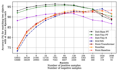
(a)

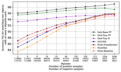
(b)

Figure 1: The performance of point cloud ReID approaches image ReID with sufficient points. We plot the performance of image and point cloud ReID networks as a function of point density. Left shows models trained on nuScenes and evaluated on nuScenes Eval set, while right shows models trained on the Waymo Open Dataset (WOD) and evaluated on Waymo Eval.

While strong ReID performance can be obtained from image data alone, even autonomous agents equipped with arrays of RGB sensors stand to benefit from the added redundancy, diversity, and complementarity offered by processing depth-sensor information for ReID. Despite this clear added benefit, however, the existing literature on re-identification from point cloud data is almost non-existent. To the best of our knowledge, [62] is the only work directly studying the problem, but they do so on a synthetic person re-identification dataset. Together with the clear motivation for leveraging ReID from point clouds for many applications, the lack of established knowledge about this problem motivates our central research question: how effective is LiDAR-based ReID compared to camera-based ReID?

While LiDAR sensors are devoid of the lighting challenges that affect cameras, they have unique challenges of their own. The primary difficulty is the sparsity of LiDAR scans and the lack of color and texture information compared to images. A network trained to re-identify objects from point clouds must rely solely on shape information. However, certain deformable objects can pose particular difficulty as their pose can change over time. An open question is whether reliable re-identification of pedestrians is even possible from raw LiDAR input without using explicit normalization schemes. Although such questions are simple, the lack of readily available high-quality datasets for re-identification from point clouds has been a serious impediment to research thus far. We address it in what follows by providing a simple recipe for creating point clouds re-identification datasets from large-scale autonomous driving datasets.

To the best of our knowledge, we are the first work to investigate object re-identification from point cloud observations. Our contributions can be summarized as follows:

• We propose RTMM, a symmetric matching head for ReID from point clouds that runs in real-time and shows improved convergence and generalization compared to a strong baseline.

• We provide a recipe for creating re-identification datasets from large-scale autonomous driving datasets and propose a performant training-time sampling algorithm.

• We are the first to establish point cloud ReID performance relative to image ReID on large-scale datasets. Our results demonstrate that point cloud ReID can approach the performance of image ReID when LiDAR observations are sufficiently dense.

• We fit a power-law to estimate the benefits of training beyond our compute budget, suggesting that an improvement of $~{}2\%$ above our strongest ReID model ($89.3$% ReID accuracy) is attainable with an order of magnitude more compute.

Our results outline a promising future for point-based object ReID, especially as depth-sensor resolution continues to increase. Upon publication, we will release the code used to collect our re-identification datasets and train our networks.

2 Related Work

This section briefly outlines areas relevant to our study of object ReID from point clouds.

2.1 Point-Processing Networks

The ability to effectively represent irregular sets of points is essential for 3D geometry processing. Respecting the symmetries of permutation invariance (PointNet) [37] and the metric space structure of raw point clouds (PointNet++) [38] were shown early on to be important priors. Subsequent works propose edge convolutions to process point clouds in CNN-style [50], a performant and efficient residual-MLP framework [33], exploiting the benefits of depth [25], using the MLP-Mixer [4], using a transformer-based architecture [57], among others. In the following study, we select three efficient models to use for our experiments: PointNet [37], DGCNN [50], and Point-Transformer [19, 57].

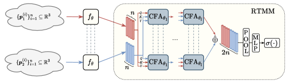
Figure 2: The architecture of our proposed symmetric matching head, RTMM.

2.2 3D Single Object Tracking

Single Object Tracking (SOT) from point clouds focuses on the task of identifying a single target object within a large search area. Consequently, most methods apply point processing networks to compare the target to the search area, which can be adapted to our point cloud ReID setting. Indeed, many recent works [13, 19, 18, 42, 39] have shown the benefits of siamese point-processing networks for SOT. Giancola et al. [13] learn a similarity function between cropped point cloud patches and use a Kalman filter to generate candidate bounding boxes for matching the current target observation. In follow-up work, P2B [39] eliminates the need to approximate greedy search at inference time in favor of an end-to-end regression approach that directly estimates the target’s next position through Hough voting. Hui et al. [18] improve on this approach with a novel regression head inspired by work on object detection [12]. In their latest work [19], the authors improve on their previous results by employing a point-transformer backbone. Given the strong performance of their architecture for SOT, we include it in our study and show that the point transformer also attains strong performance for object re-identification.

2.3 Object Re-Identification from images and point clouds

ReID from images has been an active area of research for many years, with most work focusing on Vehicle ReID [65, 60, 41, 9, 14, 11, 29, 40, 58, 23, 61] or Person ReID [63, 27, 64, 16, 32, 47, 56, 15, 59, 5, 17, 20, 21]. In contrast, ReID from point clouds has received relatively little attention. A number of works consider ReID from RGB-D data [34, 26, 28, 36], leveraging image and depth information in conjunction with skeleton normalization to improve re-identification performance in classical computer vision pipelines. In more recent work, Zheng et al. [62] propose OG-NET for pedestrian ReID from synthetic point clouds (generated from images using a human pose estimation pipeline) and RGB information. While we also use a deep neural network to process point clouds for re-identification, our study involves real observations of multiple different classes cropped directly from large-scale autonomous driving datasets.

3 Method

In the following section, we detail the architecture of our proposed Real-Time Matching Module (RTMM) for making efficient pairwise comparisons between object observations; we illustrate how existing point-based architectures can be adapted to use it, leading to a family of RTMM-based point cloud ReID networks; and we define our training objective.

3.1 A real-time matching mechanism for point sets

Given our goal of evaluating point cloud ReID in a setting that is relevant to many applications, it is important for our matching module to be capable of making a large number of pairwise comparisons (e.g., between tracks and detections from one time step to the next for multi-object tracking) in real-time. While performant architectures for comparing pairs of point clouds exist in the single object tracking literature, these methods lack an attunement to our real-time re-identification setting as they are too slow and consider an asymmetric search problem where the target and search area are not interchangeable. To construct an attuned architecture for re-identification without re-inventing the wheel, we select a state-of-the-art single object tracking method [19] and modify their “Coarse-to-Fine Correlation Network” (C2FCN), making it symmetric and real-time. We designate the resulting matching head RTMM (see fig. 2). RTMM achieves improved inference speed and generalization compared to the original C2FCN of [19](see table. 1). Moreover, RTMM’s symmetric structure improves its convergence during training, allowing it to reach a lower training loss in a shorter period of time (see Figure. 3).

Model	Match Acc.	Inference speed	Par.
C2FCN [19]	$86.39\pm 0.04$%	$92\pm 7.73$ms	$182.5$k
C2FCN no EFA	$86.19\pm 0.08$%	${\bf 6.27}\pm 1.43$ms	$91.3$k
RTMM	${\bf 86.69}\pm 0.12$%	$13.2\pm 1.48$ms	$91.3$k

Table 1: RTMM generalizes better than other approaches while being reasonably efficient. We train Point-Transformer models on WOD (over $4$ seeds) with different match heads and evaluate their performance (matching accuracy $\pm$ standard error) on Waymo Eval. Inference speed is measured for a batch of 512 examples on an RTX 3090 GPU.

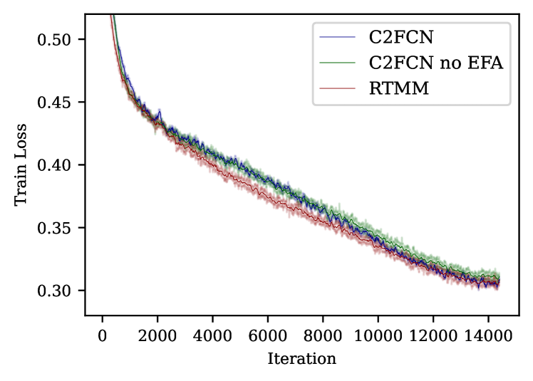
Figure 3: RTMM learns faster during training and converges to a lower training loss. Each curve is an average over $4$ trials with different seeds. Shaded regions represent one standard error from the mean.

Starting from C2FCN, we improve the module’s runtime by eliminating the ego feature augmentation module. We found that its memory and computational complexity scales poorly to a large number of comparisons (as is typical in our setting) and note that the module has little benefit to accuracy in our ReID setting. With the ego feature augmentation modules removed, only Cross-Feature Augmentation (CFA) modules remain, which are essentially linear attention blocks [22]. While we preserve the internal CFA block structure (see sec. F), we modify the interleaving of CFA modules to make a forward pass through RTMM symmetric with respect to each input. Specifically, to make symmetric comparisons between two sets of points $\{{\bm{x}}^{(i)}_{1}\}_{i}^{n_{1}},\{{\bm{x}}^{(i)}_{2}\}_{i}^{n_{2}}$, with ${\bm{x}}_{1},{\bm{x}}_{2}\in\mathbb{R}^{3}$, we apply CFA blocks symmetrically to each point cloud observation’s representation allowing each point cloud to play the role of key/value and query in turn:

$$\bar{{\bm{X}}}^{l}_{1}=\mathrm{CFA}_{\theta_{l}}(\bar{{\bm{X}}}^{l-1}_{1},{\bm{X}}_{1},\bar{{\bm{X}}}^{l-1}_{2},{\bm{X}}_{2})$$ (1)

$$\bar{{\bm{X}}}^{l}_{2}=\mathrm{CFA}_{\theta_{l}}(\bar{{\bm{X}}}^{l-1}_{2},{\bm{X}}_{2},\bar{{\bm{X}}}^{l-1}_{1},{\bm{X}}_{1}).$$ (2)

Where the two sets of points $\{{\bm{x}}^{(i)}_{1}\}_{i}^{n_{1}},\{{\bm{x}}^{(i)}_{2}\}_{i}^{n_{2}}$, are designated in stacked matrix form ${\bm{X}}_{1},{\bm{X}}_{2}\in\mathbb{R}^{n\times 3}$ (a convention we follow henceforth) and $\bar{{\bm{X}}}^{0}_{i}=f_{\theta}({\bm{X}}_{i})$ with $f_{\theta}$ being any point processing network. After being processed by $l$ CFA blocks in our symmetric formulation, outputs are concatenated along the sequence dimension to which we apply an invariant pooling operation: $\mathrm{pool}(\bar{{\bm{X}}}^{l}_{1}\hat{\oplus}\bar{{\bm{X}}}^{l}_{2})$. This differs from the original setup of [19], which only allows one point cloud to play the role of the query. Finally, an MLP is applied to the pooled representation:

$$\mathrm{RTMM}^{l}_{\theta}({\bm{X}}_{1},{\bm{X}}_{2})=\mathrm{MLP}_{res}(\mathrm{pool}(\bar{{\bm{X}}}^{l}_{1}\hat{\oplus}\bar{{\bm{X}}}^{l}_{2}))$$ (3)

where $\mathrm{MLP}_{res}$ is a residual MLP block followed by a linear projection layer, mapping each output to $\mathbb{R}$, $\mathrm{pool}({\bm{x}}):=\mathrm{maxpool}({\bm{x}})\oplus\mathrm{avgpool}({\bm{x}})$; $\hat{\oplus}$ designates sequence/set level concatenation; and $\oplus$ designates vector concatenation of the channel dimension. In practice, we find that setting $l=2$ is sufficient to achieve strong matching performance. We note that on all datasets and for all point models, we subsample or resample the input point cloud to contain $n=128$ points.

	Backbone	Par.	Acc.	F1 Pos.	F1 Neg.	Car	Pedestrian	Bicycle	Bus	Motorcycle	Truck	FP
$\overbrace{\hskip 50.0pt}^{\text{\emph{nuScenes Eval}}}$	DeiT-base∗I	$85.7$M	$92.93\%$	$92.76\%$	$93.1\%$	$95.07\%$	$89.7\%$	$89.06\%$	$91.88\%$	$90.29\%$	$92.4\%$	$96.4\%$
	DeiT-tiny∗I	$5.7$M	$91.94\%$	$91.89\%$	$91.99\%$	$94.09\%$	$88.23\%$	$89.16\%$	$90.6\%$	$89.92\%$	$92.34\%$	$94.01\%$
	DeiT-tinyI	$5.7$M	$88.15\%$	$88.19\%$	$88.12\%$	$90.34\%$	$84.42\%$	$85.63\%$	$86.85\%$	$85.81\%$	$88.52\%$	$89.58\%$
	DGCNNL	$0.6$M	$73.37\%$	$74.25\%$	$72.42\%$	$77.19\%$	$63.71\%$	$67.1\%$	$78.98\%$	$66.31\%$	$80.53\%$	$76.73\%$
	PointnetL	$2.8$M	$74.35\%$	$74.76\%$	$73.92\%$	$77.97\%$	$65\%$	$67.38\%$	$80.4\%$	$67.24\%$	$81.74\%$	$80.1\%$
	Point-TransformerL	$0.5$M	$74.54\%$	$74.72\%$	$74.35\%$	$78.36\%$	$64.39\%$	$67.24\%$	$82.62\%$	$68.08\%$	$82.48\%$	$81.04\%$
	Point-BaselineL	$0.5$M	$74.73\%$	$74.74\%$	$74.72\%$	$78.37\%$	$65.12\%$	$67.81\%$	$80.99\%$	$67.85\%$	$82.54\%$	$83.69\%$
$\overbrace{\hskip 50.0pt}^{\text{\emph{Waymo Eval}}}$	DeiT-base∗I	$85.7$M	$96.02\%$	$96\%$	$96.04\%$	$96.84\%$	$94.32\%$	$95.16\%$	$94.89\%$	$91.46\%$	$95.66\%$	$97.47\%$
	DeiT-tiny∗I	$5.7$M	$95.42\%$	$95.43\%$	$95.4\%$	$96.3\%$	$93.69\%$	$93.06\%$	$92.91\%$	$92.43\%$	$93.04\%$	$96.33\%$
	DeiT-tinyI	$5.7$M	$93.22\%$	$93.29\%$	$93.16\%$	$94.14\%$	$91.38\%$	$92.25\%$	$89.92\%$	$90.63\%$	$91.21\%$	$93.56\%$
	DGCNNL	$0.6$M	$84.92\%$	$85.03\%$	$84.81\%$	$86.86\%$	$80.56\%$	$84.12\%$	$80.99\%$	$74.69\%$	$89.47\%$	$90.3\%$
	PointnetL	$2.8$M	$83.41\%$	$83.62\%$	$83.2\%$	$85.51\%$	$78.77\%$	$82.32\%$	$80.31\%$	$74.4\%$	$85.73\%$	$88.51\%$
	Point-TransformerL	$0.5$M	$86.99\%$	$87.16\%$	$86.81\%$	$88.84\%$	$82.94\%$	$83.89\%$	$86.46\%$	$78.92\%$	$88.58\%$	$91.51\%$
	Point-BaselineL	$0.5$M	$86.09\%$	$86.37\%$	$85.79\%$	$87.93\%$	$82.15\%$	$82\%$	$84.33\%$	$78.3\%$	$86.36\%$	$92.16\%$
$\overbrace{\hskip 50.0pt}^{\text{\emph{Waymo Eval All}}}$	DeiT-base∗I	$85.7$M	$83.1\%$	$83.36\%$	$82.82\%$	$83.43\%$	$82.67\%$	$80.47\%$	$82.14\%$	$76.44\%$	$81.5\%$	$83.84\%$
	DeiT-tiny∗I	$5.7$M	$81.35\%$	$82.32\%$	$80.27\%$	$81.35\%$	$81.58\%$	$79.84\%$	$81.14\%$	$74.76\%$	$79.83\%$	$78.35\%$
	DeiT-tinyI	$5.7$M	$78.71\%$	$80.49\%$	$76.58\%$	$78.55\%$	$79.33\%$	$77.19\%$	$76.48\%$	$71.84\%$	$76.91\%$	$72.3\%$
	DGCNNL	$0.6$M	$83.15\%$	$83.24\%$	$83.05\%$	$85.49\%$	$78.22\%$	$82.26\%$	$80.46\%$	$74.05\%$	$86.46\%$	$88.41\%$
	PointnetL	$2.8$M	$81.62\%$	$81.88\%$	$81.35\%$	$84.02\%$	$76.62\%$	$81.37\%$	$78.16\%$	$72.1\%$	$83.9\%$	$85.76\%$
	Point-TransformerL	$0.5$M	$85.01\%$	$85.15\%$	$84.87\%$	$87.16\%$	$80.53\%$	$81.68\%$	$83.07\%$	$78.64\%$	$87.1\%$	$89.36\%$
	Point-BaselineL	$0.5$M	$84.3\%$	$84.48\%$	$84.1\%$	$86.29\%$	$80.27\%$	$79.16\%$	$80.71\%$	$77.35\%$	$86.03\%$	$90.39\%$

^∗: Pre-trained & fine-tuned on ImageNet 1k, ^I: using RGB data, ^L: using LiDAR data

Table 2: Image v.s. point cloud performance for object re-identification. While image models outperform their point-based counterparts, the large performance improvement from nuScenes to Waymo shows that increasing LiDAR sensor resolution can lead to significant performance improvement. Pedestrians benefit the most from this increase in sensor resolution, showing that at higher resolutions even the re-identification of deformable objects is possible without any explicit skeleton normalization step. These findings show a promising future for point cloud based re-identification as LiDAR sensor resolution continues to increase.

3.2 Compatibility with existing point backbones

In our empirical evaluation, we select $f_{\theta}$ to be PointNet [37], DGCNN [50], and Point Transformer [19]. However, almost any point processing backbone can be adapted with minimal effort to use our proposed RTMM. Due to the unstructured nature of point cloud inputs, most point-processing backbones compute an intermediate representation $f_{\theta}({\bm{X}})\in\mathbb{R}^{B\times N\times d}$ which is equivariant to permutations of the columns of ${\bm{X}}$, followed by an invariant pooling layer. Such constructions preserve the set cardinality dimension $N$ until the pooling operation, making them amenable to processing using sequence models, such as our RTMM. Therefore, many existing point backbones can be adapted to our method by extracting their representation before invariant pooling layers.

3.3 Training objective

We train our networks for object re-identification tasks using binary cross-entropy,

$$\mathcal{L}({\bm{x}},{\bm{y}})=\frac{1}{n}\sum^{n}_{i=1}({\bm{y}}_{i}\cdot\log({\bm{x}}_{i})+(1-{\bm{y}}_{i})\log(1-{\bm{x}}_{i})).$$ (4)

4 Large scale point cloud ReID Datasets

To train our point re-identification networks, we extract object observations from the nuScenes dataset [2] and the Waymo Open Dataset (WOD) [45]. This extraction process is non-trivial and seeks to maximize the applicability of our results to downstream applications, such as multi-object tracking, that identify objects using an object detector as a first step. Here, we briefly describe the salient details.

Sensors

Each dataset contains multimodal driving data captured from one (nuScenes) or multiple (WOD) LiDAR sensors and an array of camera sensors. NuScenes employs a single $360^{\circ}$ $32$-beam LiDAR, while Waymo features one $64$-beam $360^{\circ}$ $10$ Hz top-mounted sensor with four additional close proximity LiDAR sensors on the front, back, and sides of the vehicle. This means that the WOD LiDAR scans will be many times denser than their nuScenes counterparts. The situation is reversed for cameras, however. In nuScenes, there are 6 cameras that capture a full $360^{\circ}$ view of the scene, while the WOD only has 5 cameras with a front-facing FOV of $\sim 252^{\circ}$ and a corresponding blind spot behind the vehicle. These differences allow us to examine the effect of sensor resolution on ReID performance and to explore a practically relevant setting where point-based ReID trivially complements image ReID due to the camera’s blind spot.

Object Extraction

To simulate the noise encountered in a real tracking-by-detection setting we extract object observations using bounding boxes predicted by 3D object detectors. For nuScenes, we use a pre-trained BEVfusion C+L model [30], while we train our own CenterPoint model [54] for 3D object detection on WOD (see sec. A.1 for details). We post-process detections by using each model’s implementation of non-maximal suppression with default settings and further eliminate noisy detections by thresholding their confidence score to be above $\tau_{c}=0.1$. Using the remaining detections, we extract true and false positives by matching detected bounding boxes to ground truth bounding boxes using a permissive 3D Intersection over Union (IoU) threshold of $\tau_{IoU}=0.01$. Hungarian matching is used here to obtain a unique assignment between ground truth and true positive bounding boxes. Duplicate true positives are discarded. To extract observations from LiDAR scans, we first crop points within an object’s 3D bounding box before translating and rotating them such that the 3D bounding box becomes centered at $(0,0,0)^{\top}$ and faces a canonical orientation. Note that despite this normalization step, the observations will still contain realistic noise from the object detector’s prediction; that is, the object’s true orientation will not necessarily be facing the canonical orientation, nor will its true center necessarily be at $(0,0,0)^{\top}$. To extract observations from images, we project the predicted 3D bounding boxes to the image plane. Depending on its relative orientation,the bounding box may project to a non-rectangular shape. Therefore, we always use the smallest axis-aligned bounding box enclosing the projected shape. For bounding boxes that project to multiple images, we select the projection with the largest enclosing bounding box. To maintain object identities for re-identification we use the ground truth tracking labels.

Enhancing WOD Class labels

The nuScenes dataset provides a large number of class labels for their tracking dataset: car, bus, pedestrian, truck, bicycle, motorcycle, and trailer. WOD, however, provided substantially fewer tracking labels with their original dataset release: vehicle, pedestrian, and bicycle. In an effort to make the results between the two datasets more comparable, we enhance the WOD labels using their point cloud segmentation labels (released in a subsequent update to the dataset). Specifically, we annotate the objects within segmentation-annotated frames using majority voting of annotated points within their bounding boxes. Then, using the tracking labels, we propagate the new class of the object to all frames. This procedure expands the labels to include truck, bus, and motorcycle (see Fig. 6).

Sampling at training time

At training time, one epoch constitutes one pass over every unique object in the dataset. For each object $O$ (let $c$ denote the class of $O$), we flip a coin to determine whether to sample a positive or negative pair. Positive pairs are created by sampling a second observation uniformly at random from the other observations of $O$, while choosing to sample a negative pair leads to another coin toss. This time, we select between sampling a false positive FP of class $c^{\prime}$ ($c^{\prime}$ denotes a false positive misclassified by the object detector as belonging to class $c$) or a true positive by sampling an object $O^{\prime}$ of class $c$ other than $O$. In either case, we must account for point density before sampling our observation. If we were to naïvely select uniformly at random among all possible observations to create a negative pair, the distributions of point densities would be wildly different between positive and negative pairs.Intuitively, this happens because positive pairs are always sampled among observations of the same object that may be more likely to have similar numbers of points. If sampling is done naïvely, models can fit the spurious correlation created between positive samples and point density during training. To avoid this pitfall, when sampling a false or true positive observation to create a negative pair, we follow $O^{\prime}s$ categorical distribution over the point density buckets $[2^{n},2^{n+1})$ to select the bucket from which we then sample observations. This way, the positive and negative examples follow roughly the same point density distribution during training. Table 3 shows how this simple sampling algorithm which we can ”Even Sampling” improves over naïvely sampling uniformly at random. We additionally provide pseudocode for our training-time sampling procedure is detailed in algorithm 1.

Model	Uniform	Even	$\Delta$	Eval Dataset
DGCNN	$71.6$%	$73.37$%	lightgreen+1.77	Waymo Eval All
PointNet	$72.92$%	$74.35$%	lightgreen+1.43
Point-Transformer	$72.83$%	$74.54$%	lightgreen+1.71
DGCNN	$82.26$%	$84.92$%	lightgreen+2.66	nuScenes Eval
PointNet	$81.37$%	$83.41$%	lightgreen+2.04
Point-Transformer	$84.75$%	$86.99$%	lightgreen+2.24

Table 3: Even sampling improves performance for all models across both datasets.

Sampling at testing time

At testing time, we sample a balanced test set of large size that can accurately estimate the performance of our models at all point densities. To accomplish this, we sample at most $10$ distinct positive pairs ($o_{1}$,$o_{2}$) for each object in the test set, keeping track of their point densities($d_{o_{1}}$,$d_{o_{2}}$). Then, for each positive pair ($o_{1}$,$o_{2}$), we sample a corresponding negative pair ($o_{1}$,$o_{2}^{\prime}$), where $o_{2}^{\prime}$ has a similar point density to $o_{2}$. We define point densities as similar if they fall within the same power-two interval: $[2^{n},2^{n+1})$. Before sampling from the nuScenes test set, we filter out observations that have fewer than two points and observations without image crops. We name this test set nuScenes Eval. On WOD, we create two test sets. The first, called Waymo Eval, is created identically to nuScenes Eval. The second, called Waymo Eval All, only filters out observations that have fewer than two points. Therefore, it will include many observations that have no associated image crops as they are out of the sensor’s field of view, exposing the actual performance of the image models. Table 9 reports statistics of these evaluation sets.

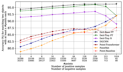
(a)

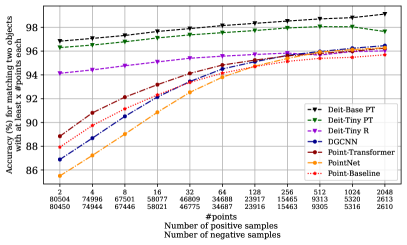
(b)

Figure 4: Deformable v.s. rigid objects. We plot the performance of models trained on WOD and evaluated on Waymo Eval as a function of point density for class pedestrian (left) and class car (right). Performance on rigid objects is much stronger than for deformable objects. However, our results show that re-identification of deformable objects can be learned directly from data without the need of explicit skeleton normalization.

5 Experiments

Our empirical evaluation is based on two re-identification datasets created from nuScenes and WOD (details provided in sec. 4). The difference in LiDAR resolution between each dataset (32 v.s. 64 beam, respectively), allows us to establish how ReID performance varies as sensor resolution increases. We also establish the relative performance of image-based and point-based ReID, show how performance varies with respect to point density within a dataset, demonstrate that increasing compute budget significantly increases our models’ performance, and fit a power-law fit to extrapolate point cloud ReID performance given more compute.

5.1 Experimental Details

To place our experiments within a meaningful context, we train three image models and one point cloud baseline model to compare with our three point cloud ReID networks (PointNet [37], DGCNN [50], and Point-Transformer [19]). For our image baselines, we select DeiT [46], a family of efficient vision transformers of different sizes. They are efficient and can be adapted with little effort to use our proposed RTMM, unlike CNNs. Specifically, we choose DeiT-Tiny as our main point of comparison and train one DeiT-Tiny model from a pre-trained checkpoint and another from random initialization. DeiT-Tiny allows us to assess the performance of an image model with a comparable number of parameters to our point models ($5$M v.s. $2.8$M). We also train a larger DeiT-Base model from a pre-trained checkpoint for reference. To compare RTMM to another matching head as a baseline, we select C2FCN no EFA due to its real-time efficiency in combination with the point-transformer backbone.

All models were trained using identical hyperparameters and the final checkpoint is used for evaluation. We used the AdamW [31] optimizer with a learning rate of $1e-5$, weight decay of $0.01$, cosine learning rate and momentum schedules [43], and gradient clipping of 2-norm $1$. We use a batch size of $256\times 4$ GPUs and $60\times 4$ GPUs for point cloud and image experiments respectively and note that our batch normalization layers were not synchronized across devices during training. Pre-trained models are trained for $200$ epochs each, while models trained from scratch are optimized for $500$ epochs and $400$ epochs on nuScenes and Waymo, respectively. The number of gradient descent steps for randomly initialized models is roughly the same ($\pm 3$ epochs) across both datasets as the Waymo dataset is larger.

5.2 A Comparison between point-based and image-based ReID

Table. 2 reports the results of our large-scale empirical study. The top section of the table corresponds to models trained on nuScenes and evaluated on nuScenes Eval. The bottom two sections correspond to models trained on Waymo and evaluated on Waymo Eval and Waymo Eval All, respectively. Matching accuracy is reported overall and for each individual class. We also report F1 scores for positive and negative matches. These results shed light on how point cloud ReID performance improves as sensor resolution is increased, how point-ReID performance varies for different objects and object categories (e.g. rigid v.s. deformable), and the performance difference between point-based and image-based object re-identification.

When comparing the accuracy of models trained on nuScenes to those trained on WOD, we observe that there is an overall increase for all models. However, the point models improve by a much greater margin than image models: as much as $12.45\%$ for the point transformer versus a $5.07\%$ increase for the randomly initialized DeiT-tiny model. We hypothesize that the performance increase of image models is due to the following reasons: 1) the image sensors are of higher resolution on WOD and 2) the WOD training set is much more diverse—it has $80\%$ more objects. This second reason is a potential confounder when assessing the extent to which the increase in point density improves point ReID performance. However, under some reasonable assumptions (see sec. C), the smaller relative increase for image models allows us to account for the confounding effect of a more diverse training set on WOD, showing that the increase in sensor resolution from nuScenes to WOD causes a performance improvement of at least $12.45\%-5.07\%=7.38\%$ for our point ReID models. This substantial increase in performance to $86.99\%$ accuracy from the top-performing Point-Transformer model shows that reasonable accuracy can be obtained from point-based ReID with enough sensor resolution.

All our models on both datasets learn an unbiased matching function on aggregate as is evidenced by similar positive and negative F1 scores. When looking at class-specific results, we note that all models follow a similar increase from nuScenes to WOD as can be observed for accuracy, except for some image models whose performance decreases on the Bus class. Of all classes, pedestrian and bicycle benefit the most from the increase in LiDAR sensor resolution with respective increases of $18.01\%$ and $14.67\%$. This is a boon for point cloud ReID’s applicability to downstream applications as it shows that the re-identification of deformable objects can be learned directly from the data when sensor resolution is sufficiently large. We note that truck and bus benefit the least from increasing LiDAR sensor resolution. We hypothesize that this is because large objects will have many points regardless of the sensor’s resolution.

Comparing the point re-identification models, Point-Transformer performs best on WOD, while all models perform very similarly on the nuScenes dataset. Focusing on image models exclusively, we note that the pre-trained DeiT-Base model performs best of all as is expected given its large number of parameters. Directly comparing point models to image models, we observe that image models always outperform their point-based counterparts when observations are visible to both camera and LiDAR sensors, but that increasing sensor resolution considerably decreases this gap. When comparing the Point-Transformer to the randomly initialized DeiT-Tiny on WOD, we observe the smallest performance gap between large rigid objects (bus, truck, and car), while the smaller deformable objects (pedestrian and bicycle) pose more difficulty to the Point-Transformer and point-based models in general. This is to be expected as deformable objects create inherent shape ambiguity, which can be resolved in images by leveraging color or texture information, but for point clouds, an object’s shape is its primary distinguishing characteristic. While the point models perform poorer than image models overall, the relative improvement seen from nuScenes to WOD is non-trivial and suggests that the gap in performance will shrink as LiDAR sensor resolution continues to increase.

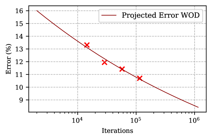
Figure 5: Extrapolating error as a function of training iterations. We fit a power-law to our training curve, yielding $\epsilon=34.5x^{-0.1}$.

	Backbone	Epochs	Acc.	F1 Pos.	F1 Neg.	Car	Pedestrian	Bicycle	Bus	Motorcycle	Truck	FP
$\overbrace{\hskip 30.0pt}^{\text{\emph{Waymo Eval}}}$	Point-TransformerL	$3200$	$89.3\%$	$89.45\%$	$89.16\%$	$90.68\%$	$86.22\%$	$87.42\%$	$89.21\%$	$84.47\%$	$90.92\%$	$92.35\%$
	Point-TransformerL	$1600$	$88.58\%$	$88.75\%$	$88.41\%$	$90.21\%$	$85\%$	$85.52\%$	$87.8\%$	$82.2\%$	$90.18\%$	$92.13\%$
	Point-TransformerL	$800$	$88.05\%$	$88.2\%$	$87.9\%$	$89.69\%$	$84.47\%$	$85.09\%$	$86.54\%$	$81.89\%$	$89.53\%$	$92.14\%$
	Point-TransformerL	$400$	$86.99\%$	$87.16\%$	$86.81\%$	$88.84\%$	$82.94\%$	$83.89\%$	$86.46\%$	$78.92\%$	$88.58\%$	$91.51\%$

^L: using LiDAR data

Table 4: Scaling compute improves performance for all classes on WOD.

5.3 Intra-dataset point density comparison

It is reasonable to expect that point cloud ReID performance will continue to increase as LiDAR sensor resolution increases. Figure 1 estimates the effect that even higher sensor resolution has on performance by plotting the accuracy of each model as a function of point density. Specifically, the accuracy (y-axis) is measured for different subsets of nuScenes Eval (left) and Waymo Eval (right) containing pairs of point cloud observations $(\{{\bm{x}}^{(i)}_{1}\}_{i}^{n_{1}},\{{\bm{x}}^{(i)}_{2}\}_{i}^{n_{2}})$, where $x\leq\min(n_{1},n_{2})$. The number of positive and negative examples for each threshold is shown on the x-axis. We observe that the magnitude of the increase is much greater for point models than image models, showing that when sufficient points are available, point cloud ReID models can approach the performance of image re-identification models. This further suggests that increasing LiDAR sensor resolution will improve point cloud ReID performance.

Figure. 4 compares the re-identification performance for deformable (pedestrian, left) and non-deformable objects (car, right) as point density is increased on Waymo Eval. For pedestrians, DGCNN and PointNet benefit the most from higher sensor resolutions, while the Point-Baseline and Point-Transformer models (both using a Point-Transformer backbone) are unable to take advantage of the highest point densities. This difficulty seems to be unique to deformable objects, however, as the car class follows a logarithmic trend of improvement with all models achieving similar performance. We note that the Point-Transformer model equipped with our proposed RTMM bests the Point-Baseline at every point density. With as few as $64$ points per object, point-based object re-identification attains performance greater than $94\%$ for all models when objects are rigid. This shows that point-based object re-identification can be extremely competitive in such settings.

6 Scaling training compute for point-based ReID

As seen in table 10 the number of samples in our ReID datasets is combinatorially large. For WOD, there are $4.35e8$ positive samples and $3.89e19$ negative samples. To put this in perspective it would take $\sim 13,646$ epochs to sample all possible positive samples on WOD while we only train our models for $400$ epochs. To provide practical estimates of attainable performance and showcase the best performance attainable we train four Point-Transformer models for $400\cdot 2^{i}$ epochs with $i\in\{0,1,2,3\}$ on the WOD and fit a power-law through their validation accuracy.

Tables 4 and 11 show the performance of models trained on progressively larger compute budgets for WOD and nuScenes, respectively. We observe a similar effect for both datasets: performance increases across the board as the compute budget is increased. Since the largest training schedules ($3200$ epochs or $115200$ iterations) on WOD only sample a small fraction of the enormous number of possible samples, we hypothesize that performance will continue to increase with more training.

Figure. 5 plots a power law fit to the error and training iterations from table 4. Specifically, we follow model $\mathcal{M}_{2}$: $\epsilon_{x}-\epsilon_{\infty}=\beta x^{c}$ from [1]. The best fit obtained was $\epsilon_{\infty}=0,\beta=34.5,c=-0.1$. This suggests that even better ReID performance is attainable by continuing to increase compute with an order of magnitude more training iterations projected to yield a model with less than 9% error. This is encouraging for applications of point-based ReID which typically require low error to be worthwhile.

7 Conclusion

We have conducted the first large-scale study of object re-identifications from point cloud observations. Our findings can be summarized as follows: 1) we propose RTMM a symmetric matching head for point cloud ReID that improves generalization and convergence, 2) we establish the performance of point cloud ReID relative to image ReID, 3) we show that our point ReID networks can attain strong ReID performance, even on par with image models, as long as the compared observations are sufficiently dense, 4) we established that point ReID performance increases as LiDAR sensor resolution is increased, 5) we demonstrated the performance of point ReID models can be substantially increased by training for longer (89%+ accuracy).

While image ReID outperforms point ReID when observations are visible to both sensors, our results show that the latter still attains strong enough performance to be useful for downstream applications. Therefore, applications can be developed that leverage this newly discovered capability. For the time being, autonomous driving systems like the WOD vehicle, which have limited camera FOV, stand to benefit the most from the added complementarity of a ReID network processing $360^{\circ}$ LiDAR scans. However, even vehicles equipped with cameras covering $360^{\circ}$ can benefit from the added redundancy of point ReID, especially in cases where the observations are sufficiently dense to be reliable. In the future, as LiDAR technology continues to advance, point ReID performance can only increase—magnifying the implications of our findings. Already today, bleeding edge LiDAR sensors feature 128 beams[44], twice the resolution of WOD’s top-mounted LiDAR.

Our initial study opens many directions for future work. Integrating our point cloud ReID models into downstream applications such as multi-object tracking for autonomous driving or robot grasping are logical next steps. Other directions include improving ReID performance by fusing LiDAR in the camera, using techniques such as [35, 49] could work well with our framework. Another interesting direction would be to study how additional geometric priors, such as SE(3) or SO(3) equivariance [8, 10] can enhance ReID from point clouds.

Supplementary Material for
Object Re-Identification from Point Clouds

Appendix A Extended experimental details

The following section contains further details of the models used to conduct our experiments.

A.1 3D object detectors

We generate our ReID datasets using point cloud samples cropped from predicted 3D bounding boxes and image samples cropped from their projections onto images. Here, we describe the details of the object detectors used to predict these bounding boxes.

Class Level 1 Level 2 mAP mAPH mAP mAPH Car 68.3 67.8 60.7 60.2 Truck 34.2 33.5 32.2 31.6 Bus 49.0 48.6 42.6 42.3 Motorcycle 53.1 52.2 38.0 37.4 Cyclist 68.4 67.0 65.8 64.5 Pedestrian 65.9 59.7 58.0 52.4

Table 5: Performance of the CenterPoint model on the WOD with enhanced vehicle labels. The metrics are only calculated on samples with an enhanced label.

Class AP ATE ASE AOE AVE AAE Car 89.2 0.170 0.148 0.061 0.274 0.185 Truck 64.6 0.326 0.181 0.093 0.247 0.217 Bus 75.3 0.338 0.189 0.069 0.430 0.274 Trailer 42.5 0.520 0.201 0.610 0.214 0.140 Const. Veh. 30.4 0.735 0.431 0.797 0.118 0.295 Pedestrian 88.2 0.134 0.288 0.387 0.217 0.101 Motorcycle 78.6 0.184 0.249 0.216 0.348 0.271 Bicycle 65.1 0.169 0.257 0.411 0.190 0.015 Traffic Cone 79.5 0.121 0.317 - - - Barrier 72.0 0.178 0.277 0.054 - - NDS: 0.714 68.5 0.288 0.254 0.300 0.255 0.187

Table 6: Performance of the BEVfusion C+L model on the nuScenes validation set. This model was used to generate the nuScenes detections for tracking and to create the nuScenes ReID dataset.

nuScenes

On the nuScenes dataset, we use BEVfusion C+L [30] to extract detections for constructing our ReID dataset. Table 6 shows its performance on the nuScenes validation set.

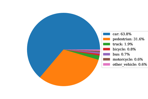
Figure 6: Waymo class label split after propagating segmentation annotations. The plot shows the proportions of different types of objects in the Waymo training set. We note that those samples belonging to the “other_vehicle” class are ignored during the creation of our ReID dataset since we do not have label information for them.

Waymo

On the Waymo dataset, we train a CenterPoint [54] object detector using the implementation from [7]. Our CenterPoint model is trained for 20 epochs, where each epoch constitutes a pass over 20% of the frames in WOD (sampled uniformly at random). Since the Waymo dataset’s Vehicle class is heterogeneous and contains various sub-types of objects that are annotated separately in the nuScenes [2] dataset, we utilize the point-wise semantic segmentation label to automatically divide the Vehicle class into {Car, Truck, Bus, Motorcycle}. Figure 6 shows the proportion of object classes after propagating segmentation labels. Our model’s evaluation results on the Waymo validation set with segmentation labels are reported in table 6.

While results between datasets are difficult to compare, we hypothesize that the nuScenes model attains relatively stronger performance. This is to be expected as the model incorporates both camera and LiDAR information, while our Waymo model does not. We note that this performance difference should have an impact on the level of noise in predicted bounding boxes and consequently may impact our ReID network’s performance.

A.2 Hyperparameters, training details, and inference speed.

Table 7 reports the hyperparameters of our ReID networks in greater detail. We note that the difference in training epochs ($400$ vs. $500$) for the Waymo and nuScenes datasets was intentional to have approximately the same number of gradient descent steps for each ($\pm 3$ epochs).

Parameter	Explanation	Value
Point model hyperparameters
B	Batch Size	$256\times 4$
N	Number of input points	$128$
$D_{p}$	Point input dimension	$3$
$\mathrm{LR}$	Learning Rate	$3\cdot 10^{-4}$
WD	weight decay	$0.01$
$\mathrm{G}_{c}$	Gradient Clipping	1
Image model hyperparameters
$D_{I}$	Image input dimension	$3\times 224\times 224$
B	Batch Size	$60\times 4$
$\mathrm{LR}$	Learning Rate	$3\cdot 10^{-5}$
WD	weight decay	$0.01$
$\mathrm{G}_{c}$	Gradient Clipping	1
Randomly initialized Waymo models
E	Training epochs	500
Randomly initialized nuScenes models
E	Training epochs	400
Pretrained Models
E	Training epochs	200

Table 7: Hyperparameters of our different architectures. Both image and point models follow a cyclic learning rate schedule with target_ratio $(10,1e-4)$, cyclic_times $1$, and step_ratio_up $0.4$ implemented by the software package MMCV [6]

Model	Par.	Batch Size	Inference Time
DeiT-Tiny	$5910$K	$100$	$32.4\text{ ms }\pm 1.75\text{ms}$
DeiT-Base	$87,338$K	$100$	$173\text{ ms }\pm 11.8\text{ms}$
Point Transformer	$529$K	$100$	$15\text{ ms }\pm 0.605\text{ms}$
DGCNN	$617$K	$100$	$18.7\text{ ms }\pm 3.25\text{ ms }$
PointNet	$2800$K	$100$	$8.04\text{ ms }\pm 0.0996\text{ ms}$
C2FCN[19]	$182.5$k	$512$	$92\pm 7.73$ ms
C2FCN no EFA	$91.3$k	$512$	$6.27\pm 1.43$ ms
RTMM	$91.3$k	$512$	$13.2\pm 1.48$ ms

Table 8: Inference speed of different point and image backbones. All models were tested on a single RTX 3090 GPU.

Table 8 reports the inference speed of all models used in our empirical evaluation. We select batch sizes to simulate the needs of practitioners in a multi-object tracking context. Backbone models are tested for a batch size of $100$, an approximate upper bound on the number of detections a 3D object detector might make at a given timestep. We test RTMM with a larger batch size of $512$, since pairwise comparisons scale quadratically with the input size. We note, however, that it is possible to considerably reduce the comparisons needed by only comparing within the same class or imposing other such rules. At the batch sizes shown, all our models, backbone + RTMM, run in real-time ($<10$ Hz), except for the DeiT-Base model.

Appendix B Additional dataset details

Table 10 reports training set statistics for both our ReID datasets, while table 9 report test set statistics. Algorithms 1 and 2 provide pseudocode for the even and uniform sampling procedures introduces in section 4 and evaluated in table 3. In algorithm 1, for a given object, the frequency distribution over power-two buckets is computed by calculating the number of observations that fall within each bucket and normalizing by the total number of observations of that object, creating a probability distribution over buckets.

Dataset	Positive Pairs	Negative Pairs	Total
nuScenes Eval	53,787	53,733	107,520
Waymo Eval	120,859	120,805	241,664
Waymo Eval All	145,458	145,358	290,816

Table 9: Evaluation set statistics.

Classes # of Obj. # of Obs. Pos. Pairs Neg. Pairs FP bicycle $--$ $13,100$ $--$ $--$ FP bus $--$ $2,069$ $--$ $--$ FP car $--$ $125,223$ $--$ $--$ FP motorcycle $--$ $7,222$ $--$ $--$ FP pedestrian $--$ $106,206$ $--$ $--$ FP trailer $--$ $8,023$ $--$ $--$ FP truck $--$ $21,792$ $--$ $--$ bicycle $554$ $7,575$ $7.76e+4$ $1.62e+12$ bus $422$ $8,375$ $1.07e+5$ $4.54e+11$ car $20,830$ $326,967$ $3.77e+6$ $3.34e+16$ motorcycle $588$ $8,201$ $8.67e+4$ $9.73e+11$ pedestrian $9,112$ $156,852$ $1.83e+6$ $5.43e+15$ trailer $773$ $13,921$ $1.66e+5$ $3.34e+12$ truck $2,933$ $50,487$ $5.98e+5$ $1.32e+14$ Total $35,212$ $856,013$ $6.63e+06$ $3.90e+16$

Classes # of Obj. # of Obs. Pos. Pairs Neg. Pairs FP bicycle $--$ $27,043$ $--$ $--$ FP bus $--$ $2,378$ $--$ $--$ FP car $--$ $24,971$ $--$ $--$ FP motorcycle $--$ $46,111$ $--$ $--$ FP pedestrian $--$ $604,021$ $--$ $--$ FP truck $--$ $5,987$ $--$ $--$ bicycle $497$ $46,204$ $3.02e+6$ $1.23e+14$ bus $378$ $43,639$ $3.35e+6$ $4.59e+13$ car $43,305$ $4,002,934$ $2.78e+8$ $3.25e+19$ motorcycle $355$ $32,317$ $2.18e+6$ $9.90e+13$ pedestrian $18,107$ $1,954,970$ $1.41e+8$ $6.40e+18$ truck $1,114$ $108,722$ $7.77e+6$ $7.13e+14$ Total $63,756$ $6,899,297$ $4.35e+08$ $3.89e+19$

Table 10: Training set statistics for nuScenes (left) and WOD (right). From left to right, the columns contain the number of unique objects of each class, the number of observations of these objects, the number of positive pairs of each class, and the number of negative pairs of each class. False positives are used to create negative pairs with observations of the corresponding true positive class. Positive and negative pairs are created from objects of the same predicted class.

Data: Dataset $D$ of all objects and their observations.

Result: A set of sampled pairs for one epoch of training.

// Initialize sample

$S\leftarrow\emptyset$; foreach object $O$ in $D$ do

       $o_{1}\leftarrow\text{random observation of }O$;

       $c\leftarrow\text{class of }O$;

       $p_{1}\leftarrow\text{random number between }0\text{ and }1$;

       if $p_{1}\leq 0.5$ then

             // Sample positive pair

             $o_{2}\leftarrow\text{random observation of }O\text{ other than }o_{1}$;

            

       end if

      else

             // Get distribution of object O

             $D\leftarrow\text{frequency distribution of power-two buckets}$

                       for O’s observations;

             $b\leftarrow\text{sample a point density bucket from $D$}$;

            [1mm] // Sample negative observation

             $p_{2}\leftarrow\text{random number between }0\text{ and }1$;

             if $p_{2}\leq 0.5$ then

                   // Sample false positive

                   $fp_{o}\leftarrow\text{random false positive of density $b$ with predicted class }c$;

                   $S\leftarrow S\cup{fp_{o}}$;

                  

             end if

            else

                   // Sample true positive

                   $o_{2}\leftarrow\text{random observation of density b with class }c$

                            $\text{ other than those associated with }O$;

                  

             end if

            

       end if

      $S\leftarrow S\cup(o_{1},o_{2})$;

      

end foreach

return $S$

Algorithm 1 Even Data Sampling Algorithm for one Epoch of Training

Data: Dataset $D$ of all objects and their observations.

Result: A set of sampled pairs for one epoch of training.

// Initialize sample

$S\leftarrow\emptyset$; foreach object $O$ in $D$ do

       $o_{1}\leftarrow\text{random observation of }O$;

       $c\leftarrow\text{class of }O$;

       $p_{1}\leftarrow\text{random number between }0\text{ and }1$;

       if $p_{1}\leq 0.5$ then

             // Sample positive pair

             $o_{2}\leftarrow\text{random observation of }O\text{ other than }o_{1}$;

            

       end if

      else

             // Sample negative observation

             $p_{2}\leftarrow\text{random number between }0\text{ and }1$;

             if $p_{2}\leq 0.5$ then

                   // Sample false positive

                   $fp_{o}\leftarrow\text{random false positive of predicted class }c$;

                   $S\leftarrow S\cup{fp_{o}}$;

                  

             end if

            else

                   // Sample true positive

                   $o_{2}\leftarrow\text{random observation of class }c$

                            $\text{ other than those associated with }O$;

                  

             end if

            

       end if

      $S\leftarrow S\cup(o_{1},o_{2})$;

      

end foreach

return $S$

Algorithm 2 Uniform Data Sampling Algorithm for one Epoch of Training

Appendix C A reasonable assumption

Section 5.2 analyses the results from table 2 and claims that the performance improvements from nuScenes to Waymo are due in part to the increase in sensor resolution between the datasets. However, Waymo is also much more diverse than nuScenes featuring $63,756$ unique objects v.s. $35,212$. This is a potential confounder since a more diverse dataset can also lead to improved performance. We claim, in the main manuscript, that under a reasonable assumption, we can obtain a lower bound on the performance improvement from nuScenes to Waymo that can be attributed to the increase in sensor resolution. The assumption is that the increased diversity from nuScenes to Waymo causes the same performance improvement (in terms of matching accuracy) for image and point cloud models alike. We believe it is reasonable to assume this since we have paired data (i.e., the point clouds and image crops are observations of the same objects). Assuming this, we can then take the performance difference from nuScenes to Waymo of the randomly initialized DeiT-Tiny model to be the increase caused by dataset diversity (as it can only be smaller than or equal to this quantity). Then, assuming no other confounders are present, we can account for the effect of a more diverse dataset by subtracting the performance improvement of the randomly initialized DeiT-Tiny model from the improvement of the point models. This is the number we report in section 5.2.

Appendix D Additional results analysis

While the main manuscript highlights the results that are central to our contributions, some secondary figures could not be included, but still provide additional infromation. We include them and a corresponding discussion here.

D.1 Scaling compute on nuScenes

Table 11 reports results for scaling compute on nuScenes. Specifically, we train four Point-Transformer models for $500\cdot 2^{i}$ epochs with $i\in\{0,1,2,3\}$. All models noticeably improve from longer training, as they do on WOD.

	Backbone	Epochs	Acc.	F1 Pos.	F1 Neg.	Car	Pedestrian	Bicycle	Bus	Motorcycle	Truck	FP
$\overbrace{\hskip 30.0pt}^{\text{\emph{nuScenes Eval}}}$	Point-TransformerL	$4000$	$77.89\%$	$77.92\%$	$77.85\%$	$82.03\%$	$67.63\%$	$71.82\%$	$84.15\%$	$71.35\%$	$84.77\%$	$83.18\%$
	Point-TransformerL	$2000$	$76.91\%$	$77.09\%$	$76.72\%$	$81.02\%$	$66.68\%$	$70.25\%$	$83.01\%$	$71.3\%$	$83.78\%$	$82.21\%$
	Point-TransformerL	$1000$	$75.67\%$	$75.92\%$	$75.41\%$	$79.45\%$	$65.79\%$	$69.82\%$	$82.27\%$	$68.97\%$	$82.94\%$	$81.43\%$
	Point-TransformerL	$500$	$74.54\%$	$74.72\%$	$74.35\%$	$78.36\%$	$64.39\%$	$67.24\%$	$82.62\%$	$68.08\%$	$82.48\%$	$81.04\%$

^L: using LiDAR data

Table 11: Scaling compute improves performance for all classes on nuScenes.

D.2 Additional analysis comparing accuracy at different point densities

Figure 7 is the twin of figure 1 from the main manuscript. Each figure plots the performance of our ReID networks on nuScenes (left) and Waymo (right) at different point densities. The difference between the two figures is seen on the x-axis. Figure 7 plots accuracy on pairs of observations with at least one observation containing $x$ points or more, while figure 1 requires that both observations in the pair have at least $x$ points. We observe that the increase in accuracy is steeper when restricting to cases where both observations have more than $x$ points. However, figure 7 shows the same trend but with a smaller slope and more samples for every $x$ value.

Similarly, figure 8 is the twin of figure 4 in the main manuscript. We see a similar trend of increased performance relative to the number of points but with a smaller slope compared to the plot which filters for both observations having more than $x$ points. Notably, performance improves faster on cars in figure 8 than it does for pedestrians, while the opposite was true in figure 4, suggesting that pairs of dense observations are needed for strong performance on deformable objects, while rigid objects can perform well with only one dense observation.

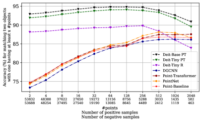
(a)

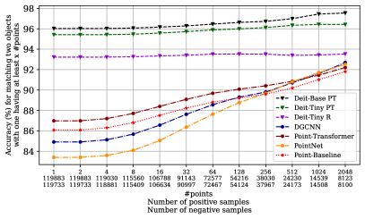
(b)

Figure 7: The performance of point cloud ReID approaches image ReID with sufficient points. The plot shows the performance of the image and point cloud ReID networks as a function of the number of points in at least one observation of the pair. Left plots models trained on nuScenes and evaluated on the nuScenes Eval set, while right plots models trained on Waymo and evaluated on Waymo Eval.

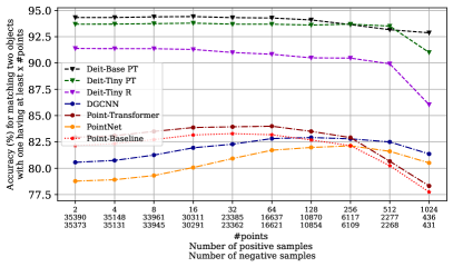
(a)

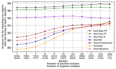
(b)

Figure 8: Deformable v.s. Non-deformable objects. The plot shows the performance of image and point cloud ReID networks for classes car and pedestrian as pairs of observations without at least one observation containing $x$ points are filtered out. We observe a similar trend for deformable and non-deformable objects: both increase with more points. However, we note that the increase in ReID performance for cars is steeper than for pedestrians. Left is evaluated on pedestrians from the Waymo Eval set, while right is evaluated on cars from Waymo Eval.

Appendix E Dataset visualization

In figures 9 and 10, we provide visual examples of samples from our Waymo ReID dataset. The images are cropped from projected 3D bounding boxes predicted by our centerpoint model (see sec. A.1 for details). The center plot shows the LiDAR point associated to the same observation. We selected observations with more than $200$ points, so that it is possible for a human to make out the underlying object. However, most of the observations contain fewer than $200$ points. The leftmost plot shows complete point clouds created by aggregating the points from all observations using ground truth bounding boxes. Aggregated deformable objects (pedestrian, bicycle, and motorcycle) have a blob-like appearance, while rigid objects retain a more detailed shape. This is due to their deformability, causing them to take on many different poses over a sequence.

Appendix F CFA block structure

Our RTMM, illustrated in Fig. 2, compares two point clouds by symmetrically applying CFA blocks [19] between them. These are linear attention blocks, but with a few modifications; here we detail the exact structure used. CFA blocks receive two sets of points $\{{\bm{x}}^{(i)}_{1}\}_{i}^{n_{1}},\{{\bm{x}}^{(i)}_{2}\}_{i}^{n_{2}}$, which we designate in stacked matrix form ${\bm{X}}_{1},{\bm{X}}_{2}\in\mathbb{R}^{n\times 3}$ henceforth, where the points are subsampled or resampled to size $n$ (we use $n=128$ for all our models), and their corresponding representations $f_{\theta}({\bm{X}}_{1}),f_{\theta}({\bm{X}}_{2})$, where $f_{\theta}$ can be any set or sequence processing network. The block first computes linear cross-attention (LCA):

$${\bm{L}}= \text{ LCA}(f_{\theta}({\bm{X}}_{1}),f_{\theta}({\bm{X}}_{2})+{\bm{P}},f_{\theta}({\bm{X}}_{2})+{\bm{P}})$$ (5)

where ${\bm{P}}=\text{ MLP}_{pos}({\bm{X}}_{2})$ is a positional encoding computed from the point cloud. Next, a layer normalization (LN) is applied followed by an MLP applied to the channel-wise concatenation of $\text{ LN}({\bm{L}})$ and $f_{\theta}({\bm{X}}_{1}))$ and another layer normalization,

$${\bm{L}}^{\prime}= \text{ LN}(\text{ MLP}(\text{ LN}({\bm{L}})\oplus f_{\theta}({\bm{X}}_{1}))).$$ (6)

Finally, a residual connection is applied to complete the CFA block:

$$\text{CFA}(f_{\theta}({\bm{X}}_{1}),{\bm{X}}_{1},f_{\theta}({\bm{X}}_{2}),{\bm{X}}_{2})= {\bm{L}}^{\prime}+f_{\theta}({\bm{X}}_{1}).$$ (7)

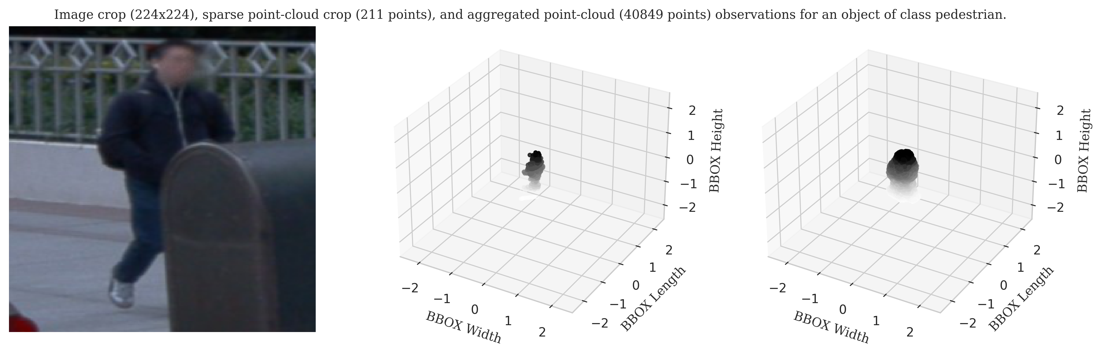
(a)

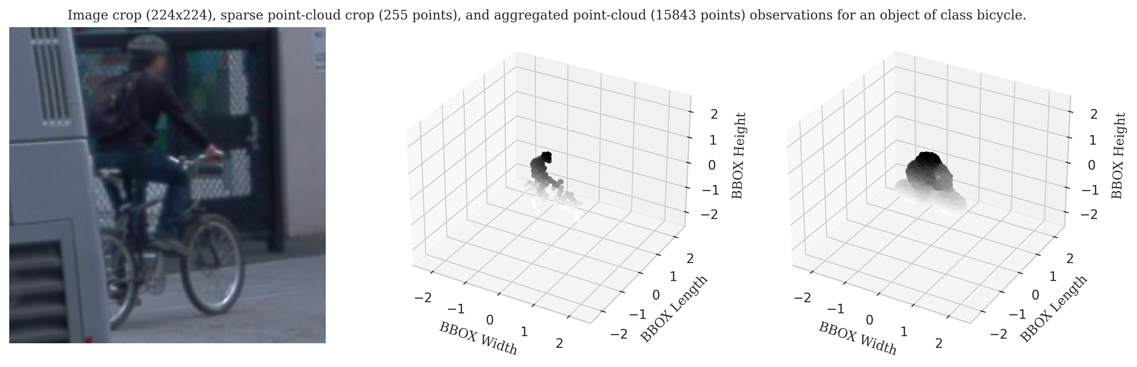
(b)

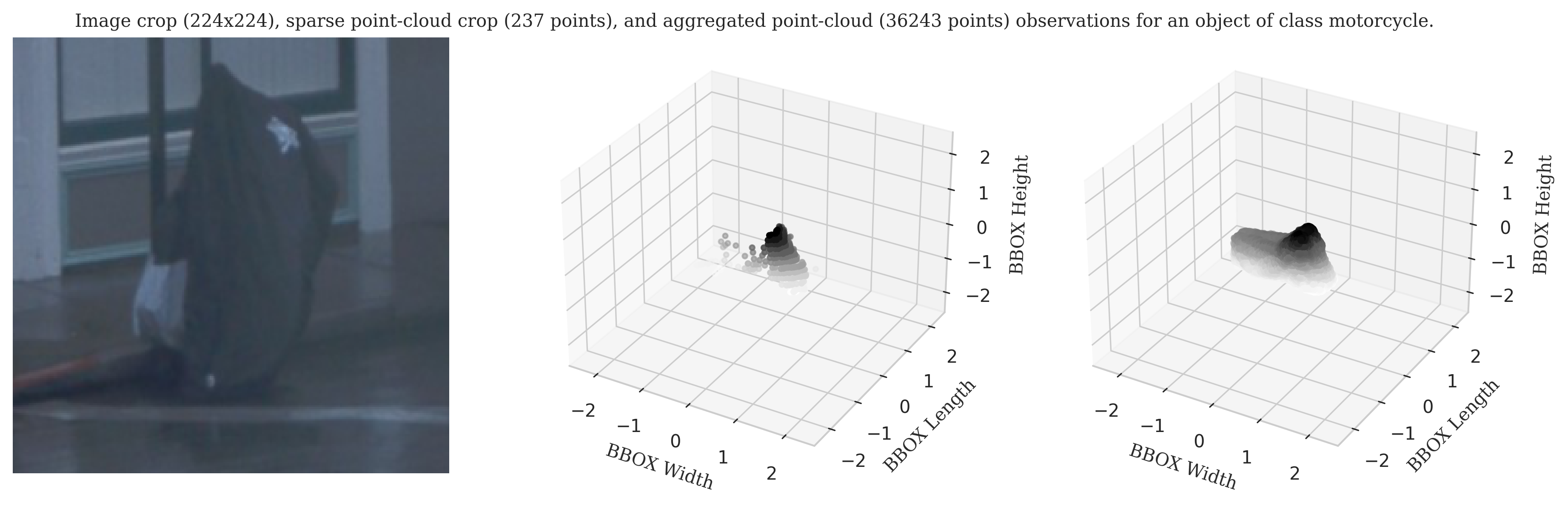
(c)

Figure 9: Samples from our Waymo ReID dataset for deformable objects. The plot shows the cropped image (left) and cropped sparse point cloud (center) for the same predicted 3D bounding box (output by our centerpoint model). We also include the corresponding complete version of the point cloud (right), created by aggregating LiDAR scans over different observations and mirroring them about the object’s center.

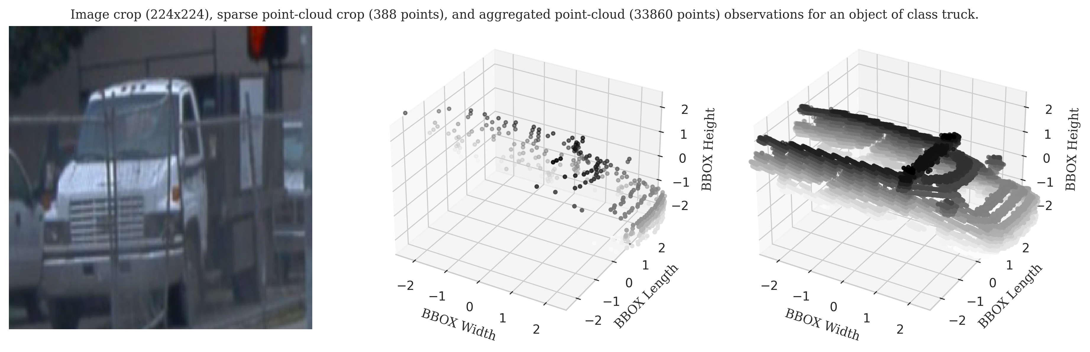
(a)

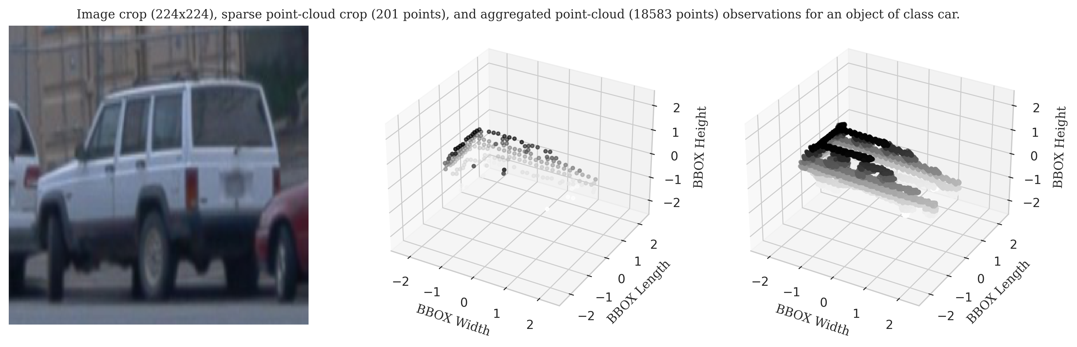
(b)

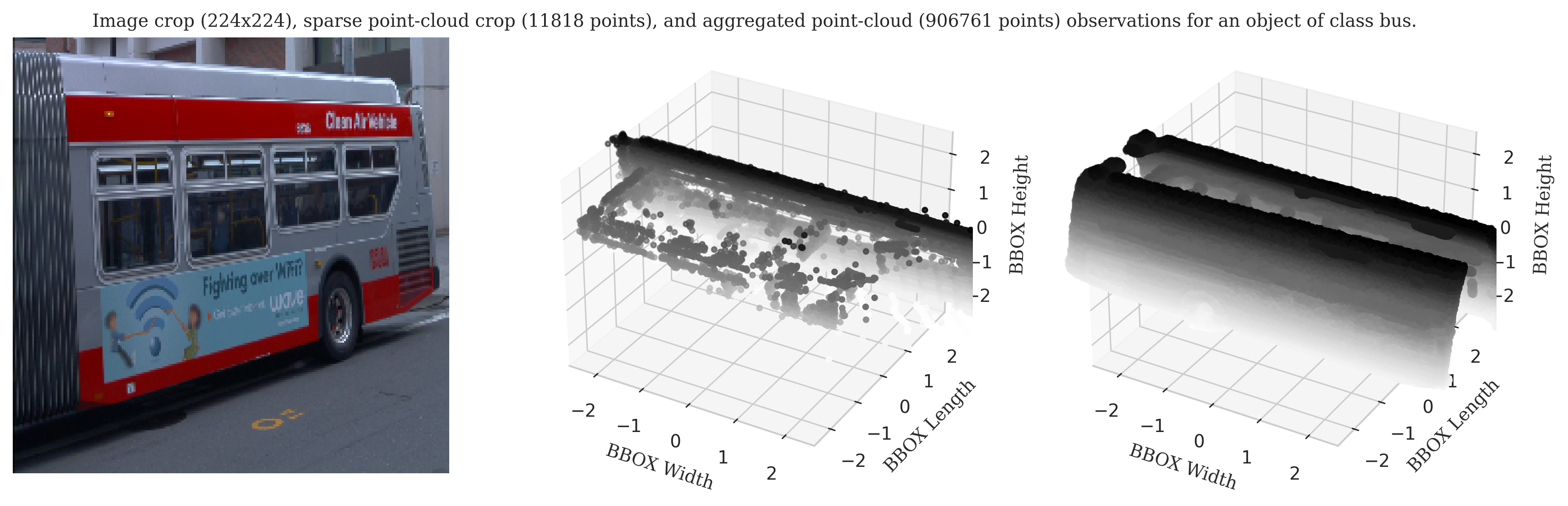
(c)

Figure 10: Samples from our Waymo ReID dataset continued for rigid objects. The plot shows the cropped image (left) and cropped sparse point cloud (center) for the same predicted 3D bounding box (output by our centerpoint model). We also include the corresponding complete version of the point cloud (right), created by aggregating LiDAR scans over different observations and mirroring them about the object’s center.

References

- [1] Ibrahim M. Alabdulmohsin, Behnam Neyshabur, and Xiaohua Zhai. Revisiting neural scaling laws in language and vision. In NeurIPS, 2022.
- [2] Holger Caesar, Varun Bankiti, Alex H. Lang, Sourabh Vora, Venice Erin Liong, Qiang Xu, Anush Krishnan, Yu Pan, Giancarlo Baldan, and Oscar Beijbom. nuscenes: A multimodal dataset for autonomous driving. In 2020 IEEE/CVF Conference on Computer Vision and Pattern Recognition, CVPR 2020, Seattle, WA, USA, June 13-19, 2020, pages 11618–11628. Computer Vision Foundation / IEEE, 2020.
- [3] Ming-Fang Chang, John Lambert, Patsorn Sangkloy, Jagjeet Singh, Slawomir Bak, Andrew Hartnett, De Wang, Peter Carr, Simon Lucey, Deva Ramanan, and James Hays. Argoverse: 3d tracking and forecasting with rich maps. In IEEE Conference on Computer Vision and Pattern Recognition, CVPR 2019, Long Beach, CA, USA, June 16-20, 2019, pages 8748–8757. Computer Vision Foundation / IEEE, 2019.
- [4] Jaesung Choe, Chunghyun Park, François Rameau, Jaesik Park, and In So Kweon. Pointmixer: Mlp-mixer for point cloud understanding. In Shai Avidan, Gabriel J. Brostow, Moustapha Cissé, Giovanni Maria Farinella, and Tal Hassner, editors, Computer Vision - ECCV 2022 - 17th European Conference, Tel Aviv, Israel, October 23-27, 2022, Proceedings, Part XXVII, volume 13687 of Lecture Notes in Computer Science, pages 620–640. Springer, 2022.
- [5] Dahjung Chung, Khalid Tahboub, and Edward J. Delp. A two stream siamese convolutional neural network for person re-identification. In IEEE International Conference on Computer Vision, ICCV 2017, Venice, Italy, October 22-29, 2017, pages 1992–2000. IEEE Computer Society, 2017.
- [6] MMCV Contributors. MMCV: OpenMMLab computer vision foundation. https://github.com/open-mmlab/mmcv, 2018.
- [7] MMDetection3D Contributors. MMDetection3D: OpenMMLab next-generation platform for general 3D object detection. https://github.com/open-mmlab/mmdetection3d, 2020.
- [8] Congyue Deng, Or Litany, Yueqi Duan, Adrien Poulenard, Andrea Tagliasacchi, and Leonidas J. Guibas. Vector neurons: A general framework for so(3)-equivariant networks. In 2021 IEEE/CVF International Conference on Computer Vision, ICCV 2021, Montreal, QC, Canada, October 10-17, 2021, pages 12180–12189. IEEE, 2021.
- [9] Viktor Eckstein, Arne Schumann, and Andreas Specker. Large scale vehicle re-identification by knowledge transfer from simulated data and temporal attention. In 2020 IEEE/CVF Conference on Computer Vision and Pattern Recognition, CVPR Workshops 2020, Seattle, WA, USA, June 14-19, 2020, pages 2626–2631. Computer Vision Foundation / IEEE, 2020.
- [10] Fabian Fuchs, Daniel E. Worrall, Volker Fischer, and Max Welling. Se(3)-transformers: 3d roto-translation equivariant attention networks. In Hugo Larochelle, Marc’Aurelio Ranzato, Raia Hadsell, Maria-Florina Balcan, and Hsuan-Tien Lin, editors, Advances in Neural Information Processing Systems 33: Annual Conference on Neural Information Processing Systems 2020, NeurIPS 2020, December 6-12, 2020, virtual, 2020.
- [11] Cunyuan Gao, Yi Hu, Yi Zhang, Rui Yao, Yong Zhou, and Jiaqi Zhao. Vehicle re-identification based on complementary features. In 2020 IEEE/CVF Conference on Computer Vision and Pattern Recognition, CVPR Workshops 2020, Seattle, WA, USA, June 14-19, 2020, pages 2520–2526. Computer Vision Foundation / IEEE, 2020.
- [12] Runzhou Ge, Zhuangzhuang Ding, Yihan Hu, Yu Wang, Sijia Chen, Li Huang, and Yuan Li. Afdet: Anchor free one stage 3d object detection. CoRR, abs/2006.12671, 2020.
- [13] Silvio Giancola, Jesus Zarzar, and Bernard Ghanem. Leveraging shape completion for 3d siamese tracking. In IEEE Conference on Computer Vision and Pattern Recognition, CVPR 2019, Long Beach, CA, USA, June 16-20, 2019, pages 1359–1368. Computer Vision Foundation / IEEE, 2019.
- [14] Shuting He, Hao Luo, Weihua Chen, Miao Zhang, Yuqi Zhang, Fan Wang, Hao Li, and Wei Jiang. Multi-domain learning and identity mining for vehicle re-identification. In 2020 IEEE/CVF Conference on Computer Vision and Pattern Recognition, CVPR Workshops 2020, Seattle, WA, USA, June 14-19, 2020, pages 2485–2493. Computer Vision Foundation / IEEE, 2020.
- [15] Shuting He, Hao Luo, Pichao Wang, Fan Wang, Hao Li, and Wei Jiang. Transreid: Transformer-based object re-identification. In 2021 IEEE/CVF International Conference on Computer Vision, ICCV 2021, Montreal, QC, Canada, October 10-17, 2021, pages 14993–15002. IEEE, 2021.
- [16] Alexander Hermans, Lucas Beyer, and Bastian Leibe. In defense of the triplet loss for person re-identification. CoRR, abs/1703.07737, 2017.
- [17] Zheng Hu, Chuang Zhu, and Gang He. Hard-sample guided hybrid contrast learning for unsupervised person re-identification. In 7th IEEE International Conference on Network Intelligence and Digital Content, IC-NIDC 2021, Beijing, China, November 17-19, 2021, pages 91–95. IEEE, 2021.
- [18] Le Hui, Lingpeng Wang, Mingmei Cheng, Jin Xie, and Jian Yang. 3d siamese voxel-to-bev tracker for sparse point clouds. In Marc’Aurelio Ranzato, Alina Beygelzimer, Yann N. Dauphin, Percy Liang, and Jennifer Wortman Vaughan, editors, Advances in Neural Information Processing Systems 34: Annual Conference on Neural Information Processing Systems 2021, NeurIPS 2021, December 6-14, 2021, virtual, pages 28714–28727, 2021.
- [19] Le Hui, Lingpeng Wang, Linghua Tang, Kaihao Lan, Jin Xie, and Jian Yang. 3d siamese transformer network for single object tracking on point clouds. In Shai Avidan, Gabriel J. Brostow, Moustapha Cissé, Giovanni Maria Farinella, and Tal Hassner, editors, Computer Vision - ECCV 2022 - 17th European Conference, Tel Aviv, Israel, October 23-27, 2022, Proceedings, Part II, volume 13662 of Lecture Notes in Computer Science, pages 293–310. Springer, 2022.
- [20] Bingliang Jiao, Lingqiao Liu, Liying Gao, Guosheng Lin, Lu Yang, Shizhou Zhang, Peng Wang, and Yanning Zhang. Dynamically transformed instance normalization network for generalizable person re-identification. In Shai Avidan, Gabriel J. Brostow, Moustapha Cissé, Giovanni Maria Farinella, and Tal Hassner, editors, Computer Vision - ECCV 2022 - 17th European Conference, Tel Aviv, Israel, October 23-27, 2022, Proceedings, Part XIV, volume 13674 of Lecture Notes in Computer Science, pages 285–301. Springer, 2022.
- [21] Xin Jin, Tianyu He, Kecheng Zheng, Zhiheng Yin, Xu Shen, Zhen Huang, Ruoyu Feng, Jianqiang Huang, Zhibo Chen, and Xian-Sheng Hua. Cloth-changing person re-identification from A single image with gait prediction and regularization. In IEEE/CVF Conference on Computer Vision and Pattern Recognition, CVPR 2022, New Orleans, LA, USA, June 18-24, 2022, pages 14258–14267. IEEE, 2022.
- [22] Angelos Katharopoulos, Apoorv Vyas, Nikolaos Pappas, and François Fleuret. Transformers are rnns: Fast autoregressive transformers with linear attention. In Proceedings of the 37th International Conference on Machine Learning, ICML 2020, 13-18 July 2020, Virtual Event, volume 119 of Proceedings of Machine Learning Research, pages 5156–5165. PMLR, 2020.
- [23] Pirazh Khorramshahi, Neehar Peri, Jun-Cheng Chen, and Rama Chellappa. The devil is in the details: Self-supervised attention for vehicle re-identification. In Andrea Vedaldi, Horst Bischof, Thomas Brox, and Jan-Michael Frahm, editors, Computer Vision - ECCV 2020 - 16th European Conference, Glasgow, UK, August 23-28, 2020, Proceedings, Part XIV, volume 12359 of Lecture Notes in Computer Science, pages 369–386. Springer, 2020.
- [24] Aleksandr Kim, Aljosa Osep, and Laura Leal-Taixé. Eagermot: 3d multi-object tracking via sensor fusion. In IEEE International Conference on Robotics and Automation, ICRA 2021, Xi’an, China, May 30 - June 5, 2021, pages 11315–11321. IEEE, 2021.
- [25] Eric-Tuan Le, Iasonas Kokkinos, and Niloy J. Mitra. Going deeper with lean point networks. In 2020 IEEE/CVF Conference on Computer Vision and Pattern Recognition, CVPR 2020, Seattle, WA, USA, June 13-19, 2020, pages 9500–9509. Computer Vision Foundation / IEEE, 2020.
- [26] Daniele Liciotti, Marina Paolanti, Emanuele Frontoni, Adriano Mancini, and Primo Zingaretti. Person re-identification dataset with RGB-D camera in a top-view configuration. In Kamal Nasrollahi, Cosimo Distante, Gang Hua, Andrea Cavallaro, Thomas B. Moeslund, Sebastiano Battiato, and Qiang Ji, editors, Video Analytics. Face and Facial Expression Recognition and Audience Measurement - Third International Workshop, VAAM 2016, and Second International Workshop, FFER 2016, Cancun, Mexico, December 4, 2016, Revised Selected Papers, volume 10165 of Lecture Notes in Computer Science, pages 1–11. Springer, 2016.
- [27] Yutian Lin, Liang Zheng, Zhedong Zheng, Yu Wu, Zhilan Hu, Chenggang Yan, and Yi Yang. Improving person re-identification by attribute and identity learning. Pattern Recognit., 95:151–161, 2019.
- [28] Hong Liu, Liang Hu, and Liqian Ma. Online RGB-D person re-identification based on metric model update. CAAI Trans. Intell. Technol., 2(1):48–55, 2017.
- [29] Kai Liu, Zheng Xu, Zhaohui Hou, Zhicheng Zhao, and Fei Su. Further non-local and channel attention networks for vehicle re-identification. In 2020 IEEE/CVF Conference on Computer Vision and Pattern Recognition, CVPR Workshops 2020, Seattle, WA, USA, June 14-19, 2020, pages 2494–2500. Computer Vision Foundation / IEEE, 2020.
- [30] Zhijian Liu, Haotian Tang, Alexander Amini, Xinyu Yang, Huizi Mao, Daniela Rus, and Song Han. Bevfusion: Multi-task multi-sensor fusion with unified bird’s-eye view representation. CoRR, abs/2205.13542, 2022.
- [31] Ilya Loshchilov and Frank Hutter. Decoupled weight decay regularization. In 7th International Conference on Learning Representations, ICLR 2019, New Orleans, LA, USA, May 6-9, 2019. OpenReview.net, 2019.
- [32] Hao Luo, Youzhi Gu, Xingyu Liao, Shenqi Lai, and Wei Jiang. Bag of tricks and a strong baseline for deep person re-identification. In IEEE Conference on Computer Vision and Pattern Recognition Workshops, CVPR Workshops 2019, Long Beach, CA, USA, June 16-20, 2019, pages 1487–1495. Computer Vision Foundation / IEEE, 2019.
- [33] Xu Ma, Can Qin, Haoxuan You, Haoxi Ran, and Yun Fu. Rethinking network design and local geometry in point cloud: A simple residual MLP framework. In The Tenth International Conference on Learning Representations, ICLR 2022, Virtual Event, April 25-29, 2022. OpenReview.net, 2022.
- [34] Matteo Munaro, Andrea Fossati, Alberto Basso, Emanuele Menegatti, and Luc Van Gool. One-shot person re-identification with a consumer depth camera. In Shaogang Gong, Marco Cristani, Shuicheng Yan, and Chen Change Loy, editors, Person Re-Identification, Advances in Computer Vision and Pattern Recognition, pages 161–181. Springer, 2014.
- [35] Arsha Nagrani, Shan Yang, Anurag Arnab, Aren Jansen, Cordelia Schmid, and Chen Sun. Attention bottlenecks for multimodal fusion. In Marc’Aurelio Ranzato, Alina Beygelzimer, Yann N. Dauphin, Percy Liang, and Jennifer Wortman Vaughan, editors, Advances in Neural Information Processing Systems 34: Annual Conference on Neural Information Processing Systems 2021, NeurIPS 2021, December 6-14, 2021, virtual, pages 14200–14213, 2021.
- [36] Cosimo Patruno, Roberto Marani, Grazia Cicirelli, Ettore Stella, and Tiziana D’Orazio. People re-identification using skeleton standard posture and color descriptors from RGB-D data. Pattern Recognit., 89:77–90, 2019.
- [37] Charles Ruizhongtai Qi, Hao Su, Kaichun Mo, and Leonidas J. Guibas. Pointnet: Deep learning on point sets for 3d classification and segmentation. In 2017 IEEE Conference on Computer Vision and Pattern Recognition, CVPR 2017, Honolulu, HI, USA, July 21-26, 2017, pages 77–85. IEEE Computer Society, 2017.
- [38] Charles Ruizhongtai Qi, Li Yi, Hao Su, and Leonidas J. Guibas. Pointnet++: Deep hierarchical feature learning on point sets in a metric space. In Isabelle Guyon, Ulrike von Luxburg, Samy Bengio, Hanna M. Wallach, Rob Fergus, S. V. N. Vishwanathan, and Roman Garnett, editors, Advances in Neural Information Processing Systems 30: Annual Conference on Neural Information Processing Systems 2017, December 4-9, 2017, Long Beach, CA, USA, pages 5099–5108, 2017.
- [39] Haozhe Qi, Chen Feng, Zhiguo Cao, Feng Zhao, and Yang Xiao. P2B: point-to-box network for 3d object tracking in point clouds. In 2020 IEEE/CVF Conference on Computer Vision and Pattern Recognition, CVPR 2020, Seattle, WA, USA, June 13-19, 2020, pages 6328–6337. Computer Vision Foundation / IEEE, 2020.
- [40] Wen Qian, Hao Luo, Silong Peng, Fan Wang, Chen Chen, and Hao Li. Unstructured feature decoupling for vehicle re-identification. In Shai Avidan, Gabriel J. Brostow, Moustapha Cissé, Giovanni Maria Farinella, and Tal Hassner, editors, Computer Vision - ECCV 2022 - 17th European Conference, Tel Aviv, Israel, October 23-27, 2022, Proceedings, Part XIV, volume 13674 of Lecture Notes in Computer Science, pages 336–353. Springer, 2022.
- [41] Clint Sebastian, Raffaele Imbriaco, Egor Bondarev, and Peter H. N. de With. Dual embedding expansion for vehicle re-identification. In 2020 IEEE/CVF Conference on Computer Vision and Pattern Recognition, CVPR Workshops 2020, Seattle, WA, USA, June 14-19, 2020, pages 2475–2484. Computer Vision Foundation / IEEE, 2020.
- [42] Jiayao Shan, Sifan Zhou, Yubo Cui, and Zheng Fang. Real-time 3d single object tracking with transformer. CoRR, abs/2209.00860, 2022.
- [43] Leslie N Smith and Nicholay Topin. Super-convergence: Very fast training of neural networks using large learning rates. In Artificial intelligence and machine learning for multi-domain operations applications, volume 11006, pages 369–386. SPIE, 2019.
- [44] Autonomous Stuff. Alpha prime, powering safe autonomy.
- [45] Pei Sun, Henrik Kretzschmar, Xerxes Dotiwalla, Aurelien Chouard, Vijaysai Patnaik, Paul Tsui, James Guo, Yin Zhou, Yuning Chai, Benjamin Caine, Vijay Vasudevan, Wei Han, Jiquan Ngiam, Hang Zhao, Aleksei Timofeev, Scott Ettinger, Maxim Krivokon, Amy Gao, Aditya Joshi, Yu Zhang, Jonathon Shlens, Zhifeng Chen, and Dragomir Anguelov. Scalability in perception for autonomous driving: Waymo open dataset. In 2020 IEEE/CVF Conference on Computer Vision and Pattern Recognition, CVPR 2020, Seattle, WA, USA, June 13-19, 2020, pages 2443–2451. Computer Vision Foundation / IEEE, 2020.
- [46] Hugo Touvron, Matthieu Cord, Matthijs Douze, Francisco Massa, Alexandre Sablayrolles, and Hervé Jégou. Training data-efficient image transformers & distillation through attention. In Marina Meila and Tong Zhang, editors, Proceedings of the 38th International Conference on Machine Learning, ICML 2021, 18-24 July 2021, Virtual Event, volume 139 of Proceedings of Machine Learning Research, pages 10347–10357. PMLR, 2021.
- [47] Guanshuo Wang, Yufeng Yuan, Xiong Chen, Jiwei Li, and Xi Zhou. Learning discriminative features with multiple granularities for person re-identification. In Susanne Boll, Kyoung Mu Lee, Jiebo Luo, Wenwu Zhu, Hyeran Byun, Chang Wen Chen, Rainer Lienhart, and Tao Mei, editors, 2018 ACM Multimedia Conference on Multimedia Conference, MM 2018, Seoul, Republic of Korea, October 22-26, 2018, pages 274–282. ACM, 2018.
- [48] Li Wang, Xinyu Zhang, Wenyuan Qin, Xiaoyu Li, Lei Yang, Zhiwei Li, Lei Zhu, Hong Wang, Jun Li, and Huaping Liu. CAMO-MOT: combined appearance-motion optimization for 3d multi-object tracking with camera-lidar fusion. CoRR, abs/2209.02540, 2022.
- [49] Yikai Wang, Wenbing Huang, Fuchun Sun, Tingyang Xu, Yu Rong, and Junzhou Huang. Deep multimodal fusion by channel exchanging. In Hugo Larochelle, Marc’Aurelio Ranzato, Raia Hadsell, Maria-Florina Balcan, and Hsuan-Tien Lin, editors, Advances in Neural Information Processing Systems 33: Annual Conference on Neural Information Processing Systems 2020, NeurIPS 2020, December 6-12, 2020, virtual, 2020.
- [50] Yue Wang, Yongbin Sun, Ziwei Liu, Sanjay E. Sarma, Michael M. Bronstein, and Justin M. Solomon. Dynamic graph CNN for learning on point clouds. ACM Trans. Graph., 38(5):146:1–146:12, 2019.
- [51] Yuchen Wei, Son N. Tran, Shuxiang Xu, Byeong Ho Kang, and Matthew Springer. Deep learning for retail product recognition: Challenges and techniques. Comput. Intell. Neurosci., 2020:8875910:1–8875910:23, 2020.
- [52] Xinshuo Weng, Yongxin Wang, Yunze Man, and Kris M. Kitani. GNN3DMOT: graph neural network for 3d multi-object tracking with 2d-3d multi-feature learning. In 2020 IEEE/CVF Conference on Computer Vision and Pattern Recognition, CVPR 2020, Seattle, WA, USA, June 13-19, 2020, pages 6498–6507. Computer Vision Foundation / IEEE, 2020.
- [53] John Willes, Cody Reading, and Steven L. Waslander. Intertrack: Interaction transformer for 3d multi-object tracking. CoRR, abs/2208.08041, 2022.
- [54] Tianwei Yin, Xingyi Zhou, and Philipp Krähenbühl. Center-based 3d object detection and tracking. In IEEE Conference on Computer Vision and Pattern Recognition, CVPR 2021, virtual, June 19-25, 2021, pages 11784–11793. Computer Vision Foundation / IEEE, 2021.
- [55] Andy Zeng, Shuran Song, Kuan-Ting Yu, Elliott Donlon, Francois Robert Hogan, Maria Bauzá, Daolin Ma, Orion Taylor, Melody Liu, Eudald Romo, Nima Fazeli, Ferran Alet, Nikhil Chavan Dafle, Rachel M. Holladay, Isabella Morona, Prem Qu Nair, Druck Green, Ian H. Taylor, Weber Liu, Thomas A. Funkhouser, and Alberto Rodriguez. Robotic pick-and-place of novel objects in clutter with multi-affordance grasping and cross-domain image matching. In 2018 IEEE International Conference on Robotics and Automation, ICRA 2018, Brisbane, Australia, May 21-25, 2018, pages 1–8. IEEE, 2018.
- [56] Kaiwei Zeng, Munan Ning, Yaohua Wang, and Yang Guo. Hierarchical clustering with hard-batch triplet loss for person re-identification. In 2020 IEEE/CVF Conference on Computer Vision and Pattern Recognition, CVPR 2020, Seattle, WA, USA, June 13-19, 2020, pages 13654–13662. Computer Vision Foundation / IEEE, 2020.
- [57] Hengshuang Zhao, Li Jiang, Jiaya Jia, Philip H. S. Torr, and Vladlen Koltun. Point transformer. In 2021 IEEE/CVF International Conference on Computer Vision, ICCV 2021, Montreal, QC, Canada, October 10-17, 2021, pages 16239–16248. IEEE, 2021.
- [58] Jianan Zhao, Fengliang Qi, Guangyu Ren, and Lin Xu. Phd learning: Learning with pompeiu-hausdorff distances for video-based vehicle re-identification. In IEEE Conference on Computer Vision and Pattern Recognition, CVPR 2021, virtual, June 19-25, 2021, pages 2225–2235. Computer Vision Foundation / IEEE, 2021.
- [59] Meng Zheng, Srikrishna Karanam, Ziyan Wu, and Richard J. Radke. Re-identification with consistent attentive siamese networks. In IEEE Conference on Computer Vision and Pattern Recognition, CVPR 2019, Long Beach, CA, USA, June 16-20, 2019, pages 5735–5744. Computer Vision Foundation / IEEE, 2019.
- [60] Zhedong Zheng, Minyue Jiang, Zhigang Wang, Jian Wang, Zechen Bai, Xuanmeng Zhang, Xin Yu, Xiao Tan, Yi Yang, Shilei Wen, and Errui Ding. Going beyond real data: A robust visual representation for vehicle re-identification. In 2020 IEEE/CVF Conference on Computer Vision and Pattern Recognition, CVPR Workshops 2020, Seattle, WA, USA, June 14-19, 2020, pages 2550–2558. Computer Vision Foundation / IEEE, 2020.
- [61] Zhedong Zheng, Tao Ruan, Yunchao Wei, Yi Yang, and Tao Mei. Vehiclenet: Learning robust visual representation for vehicle re-identification. IEEE Trans. Multim., 23:2683–2693, 2021.
- [62] Zhedong Zheng, Xiaohan Wang, Nenggan Zheng, and Yi Yang. Parameter-efficient person re-identification in the 3d space. IEEE Transactions on Neural Networks and Learning Systems, pages 1–14, 2022.
- [63] Zhedong Zheng, Xiaodong Yang, Zhiding Yu, Liang Zheng, Yi Yang, and Jan Kautz. Joint discriminative and generative learning for person re-identification. In IEEE Conference on Computer Vision and Pattern Recognition, CVPR 2019, Long Beach, CA, USA, June 16-20, 2019, pages 2138–2147. Computer Vision Foundation / IEEE, 2019.
- [64] Zhedong Zheng, Liang Zheng, and Yi Yang. A discriminatively learned CNN embedding for person reidentification. ACM Trans. Multim. Comput. Commun. Appl., 14(1):13:1–13:20, 2018.
- [65] Xiangyu Zhu, Zhenbo Luo, Pei Fu, and Xiang Ji. Voc-reid: Vehicle re-identification based on vehicle-orientation-camera. CoRR, abs/2004.09164, 2020.