Shielded Representations: Protecting Sensitive Attributes Through Iterative Gradient-Based Projection

Abstract

Natural language processing models tend to learn and encode social biases present in the data. One popular approach for addressing such biases is to eliminate encoded information from the model’s representations. However, current methods are restricted to removing only linearly encoded information. In this work, we propose Iterative Gradient-Based Projection (IGBP), a novel method for removing non-linear encoded concepts from neural representations. Our method consists of iteratively training neural classifiers to predict a particular attribute we seek to eliminate, followed by a projection of the representation on a hypersurface, such that the classifiers become oblivious to the target attribute. We evaluate the effectiveness of our method on the task of removing gender and race information as sensitive attributes. Our results demonstrate that IGBP is effective in mitigating bias through intrinsic and extrinsic evaluations, with minimal impact on downstream task accuracy.

1 Introduction

The increasing reliance on natural language processing models in decision-making systems has led to a renewed focus on the potential biases that these models may encode. Recent studies have demonstrated that word embeddings exhibit gender bias in their associations of professions Bolukbasi et al. (2016); Caliskan et al. (2017) and that learned representations of language models capture demographic data about the writer of the text, such as race or age Blodgett et al. (2016); Elazar and Goldberg (2018). Model decisions can be affected by these encoded biases and irrelevant attributes, leading to a wide range of inequities toward certain demographics. For example, a model designed to review job resumes should not factor in the applicants’ gender or race. Consequently, it is desirable to be able to manipulate the type of data encoded within text representations and to exclude any sensitive information in order to create more fair and equitable models.

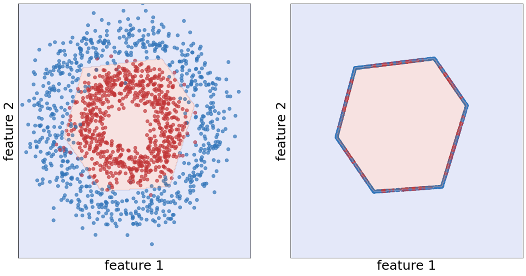
Figure 1: Left: Non-linear decision boundary of a ReLU 2-layer neural network on a binary classification task. Right: One iteration of IGBP algorithm produces clean, indistinguishable samples.

Removing the presence of sensitive attributes from the representations learned by deep neural networks is non-trivial, as these representations are often learned using complex and hard-to-interpret non-linear models. Re-training the language model can be a costly solution, therefore post-hoc removal methods that work at the representation layer have been proposed, such as linear projection of the embeddings on a hyperplane that distinguishes between the sensitive attribute Bolukbasi et al. (2016); Ravfogel et al. (2020). However, neural networks do not necessarily represent concepts in a linear manner. To address this issue, Ravfogel et al. (2022b) proposed kernelization of a linear minimax game for concept erasure, but this approach is restricted to the selection of kernel and the attribute protection does not transfer to different types of non-linear probes. Accordingly, Ravfogel et al. (2022a, b) considered non-linear concept erasure to be an open problem.

In this paper, we propose a non-linear concept erasure method, IGBP, to eliminate information about the protected attribute from neural representations. We use a trained probe classifier that attempts to predict the protected attribute and a novel loss function suited for the task of concept removal. Then, we leverage the gradients of this loss to guide for projection of the representations to a hypersurface that does not contain information used by the classifier regarding the sensitive-attribute. This is done by projecting the representations to the separating boundary of the classifier. Figure 1 illustrates a 2-dimensional example.

Our approach supports the use of non-linear neural classifiers. When used with a linear classifier, it is equivalent to Iterative Null Space Projection (INLP), a popular linear concept removal method (Ravfogel et al., 2020).

We perform an empirical evaluation of the proposed method using: (1) intrinsic evaluation of word embeddings measuring word-level gender bias removal and (2) extrinsic fair classification evaluation over tasks that uses contextualized word representations. The empirical results show that the proposed method is successful in sensitive-attribute removal and mitigating bias, outperforming competing algorithms with minimal impact on the downstream task accuracy.

2 Related Work

Many studies (e.g., Caliskan et al., 2017; Rudinger et al., 2018) investigated social biases in word embeddings and text representations. Recent work have showed how applications that use pre-trained representations reflect and amplify these kinds of social biases Zhao et al. (2018); Elazar and Goldberg (2018).

The approaches tackling this problem can be categorized into three lines of work: pre-processing methods which manipulate the input distribution before training (e.g., Zhao et al., 2018; Wang et al., 2019), in-processing methods which focus on learning fair models during training (e.g., Xie et al., 2017; Beutel et al., 2017; Zhang et al., 2018; Orgad and Belinkov, 2023) and post-hoc methods (e.g., Ravfogel et al., 2020; Wang et al., 2020; Ravfogel et al., 2022a, b), which assume a fixed, pre-trained set of representations from any encoder and aim to learn a new set of unbiased representations.

Since re-training a model can be costly, a lot of focus was given to post-hoc methods, which is the main focus of this work.

The most common post-hoc approach to remove sensitive information from word embeddings is to use a linear projection. Bolukbasi et al. (2016) identified a gender subspace, which is a subspace spanned by the directions of embeddings that capture the bias, such as the direction “he” – “she”. They suggested projecting all the gender-neutral word embeddings on the gender subspace’s first principle component to make neutral words equally distant from male and female-gendered words. However, Gonen and Goldberg (2019) showed that this method only covers up bias and not fully removes it from the representation. Another critical drawback of the method is that it requires user selection of a few gender directions.

Ravfogel et al. (2020) tried to overcome this drawback of manually defining gender direction, and presented the Iterative Null-space Projection (INLP) method. It is based on training linear classifiers that predict the attribute they wish to remove, then projecting the representations on the classifiers’ null-space. Ravfogel et al. (2022a) aims to linearly remove information from neural representations by using a linear minimax game-based approach, and derive a closed-form solution for certain objectives. One of the limitations of linear removal methods is their inability to remove non-linear information about the protected attribute, which is often encoded in text representations through complex neural networks. In contrast, our method is capable of removing both linear and non-linear information, resulting in a more effective reduction of extrinsic bias (Section 4.4).

Ravfogel et al. (2022b) proposed a nonlinear extension of the concept-removal objective of Ravfogel et al. (2022a). They identify the subspace to be neutralized in kernel space by running a kernelized version of a minimax game as in Ravfogel et al. (2022a). Shao et al. (2023) also use kernels to try and remove non-linear information While this approach aims to remove non-linear information, it can only choose data mapping from a pre-defined set of kernels, and as shown in Ravfogel et al. (2022a), the attribute protection does not transfer to other non-linear kernels . Our approach uses a deep neural network as the bias signal modeling, thus has the potential to express any non-linear function. Our empirical results (Section 4) show that our method significantly outperforms these methods on a variety of tasks.

3 Approach

3.1 Problem Formulation

Given a dataset $D=\{x_{i},y_{i},z_{i}\}_{i=1}^{N}$ which consists of triples of text representation $x_{i}\in\mathcal{X}$, downstream task label $y_{i}\in\mathcal{Y}$ and a protected attribute $z_{i}\in\mathcal{Z}$ which corresponds to discrete attribute values, such as gender. Our goal is to eliminate the information related to the protected attribute from the representations while minimizing the effect on other relevant information. To achieve this, we intend to learn a non-linear transformation of the representations such that the protected attribute $z_{i}$ cannot be inferred from the transformed representations $x^{clean}_{i}$, while still preserving the information with regard to the downstream task label $y_{i}$.

3.2 Adversarial Approach Background

The core of our approach is to produce projection of the representations such that any classifier is unable to distinguish between the protected attribute groups. To gain some intuition about how such projections are generated, let us first consider a trained probe classifier $f$ that classifies the attribute label $z$ of each representation vector $x$. By assigning adversarial perturbations and moving in the direction of the gradient of the loss function with respect to the input vector, the representations can be modified such that the classifier’s ability to predict the protected attribute is hindered, while minimizing the alteration of other relevant information:

$$x_{new}=x+\lambda\cdot\nabla_{x}L(f(x),z),$$ (1)

where $\lambda>0$. Elazar and Goldberg (2018) applied a similar approach in removal of demographic attributes from text data during training. In contrast, we apply our method on the representation layer post-training, with a specific loss function and $\lambda$.

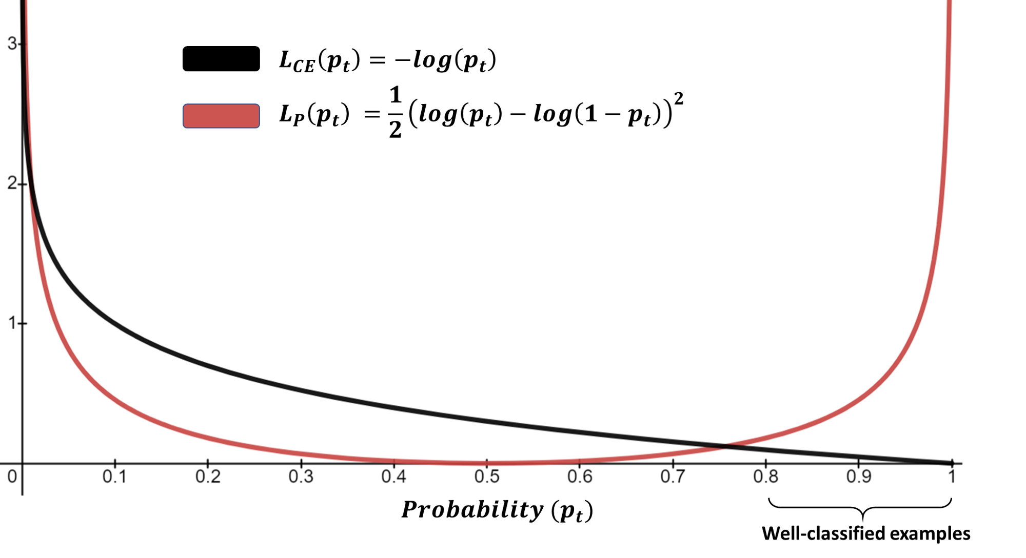
Figure 2: Cross entropy loss (black) and the projective loss (red) behavior as a function of the probability of the probe classifier given an embedding. The projective loss emphasizes the well-classified, biased embeddings.

We present a novel loss for $L$, to which we call the projective loss. It is designed for removing information from neural representation. It allows for a single-step projection of the representations, rendering the probe classifier $f$ oblivious to the protected attribute. Before presenting the projective loss, we explore why the common cross entropy (CE) is not optimal for our task. The CE loss function is defined as:

$$L_{CE}(p,y)=\begin{cases}-log(p)&\text{if y=1}\\ -log(1-p)&\text{otherwise.}\end{cases}$$ (2)

where $y\in\{\pm 1\}$ specifies the ground-truth class and $p\in[0,1]$ is the model’s estimated probability for the class with label $y=1$. For the sake of clarity, we formally define $p_{t}$:

$$p_{t}=\begin{cases}p&\text{if y=1}\\ 1-p&\text{otherwise.}\end{cases}$$ (3)

and rewrite $CE(p,y)=CE(p_{t})=-log(p_{t})$.
The CE loss can be seen in black in Figure 2. A noteworthy characteristic of this loss is that examples which are considered to have a strong signal of the protected attribute (i.e., are easily classified with $p_{t}\gg 0.5$) yield low gradients. In Appendix B we demonstrate mathematically that:

$$\nabla_{x}L_{CE}=\pm\>(1-p_{t})\nabla_{x}f^{\top}\\$$ (4)

As $p_{t}$ approaches 1, $\nabla_{x}L_{CE}$ tends to $0$ and the adversarial perturbation associated with the most-biased samples is vanishingly small. Hence, the use of gradients of the CE loss for information removal brings about a major disadvantage.

3.3 Projective Loss

A more effective way to remove the entire signal of bias in the representations would be projecting them on the hypersurface where the classifier is oblivious to the protected attribute. To achieve this, we propose the projective loss:

$$L_{P}(p_{t})=\frac{1}{2}(log(p_{t})-log(1-p_{t}))^{2}$$ (5)

Figure 2 illustrates the behavior of the projective loss compared to the more common cross entropy loss. As can be observed, the projective loss gives higher weights to examples where the probe classifier can predict the protected attribute well. The minimum occurs at $p_{t}=0.5$, where there is ambiguity for the probe classifier in determining the label. Eq. 1 is now modified as :

$$x_{p}=x-\lambda_{P}\cdot\nabla_{x}L_{P}(f(x),z),$$ (6)

The gradient of the projective loss can be expressed as:

$$\nabla_{x}L_{P}=f(x)\nabla_{x}f^{\top}$$ (7)

We show in Appendix C that Eq. 6 with the projective loss and a specific $\lambda_{P}=\frac{1}{\|\nabla_{x}f\|^{2}}$ yields a projection of the embedding vectors on the local linear model of each embedding.

Special Case of a Linear Probe Classifier.

We now analyze the special case where $f$ is a linear classifier. Given a linear classifier $f(x)=x^{\top}\theta$ where $\theta\in\mathbb{R}^{d}$ and a logistic function $\sigma(f)=\frac{1}{1+e^{-x^{\top}\theta}}$ to produce the probability $p_{t}$, we calculate the gradients of the projective loss as:

$$\nabla_{x}L_{P}=(x^{\top}\theta)\theta^{\top}$$ (8)

Normalizing $\theta$ by setting $\lambda_{P}=\frac{1}{\|\nabla_{x}f\|^{2}}=\frac{1}{\theta^{\top}\theta}$ in Eq. 6 yields the orthogonal projection formula:

$$x_{p}=x-(\frac{x^{\top}\theta}{\theta^{\top}\theta})\theta^{\top}$$ (9)

This is also known as the null space projection which is used in INLP Ravfogel et al. (2020). INLP is a special case of our method when using a linear probe classifier. Unlike INLP, which obtains the projected embeddings by identifying the null space of a linear classifier, our method utilizes the gradients of neural network classifiers to obtain the projected embeddings.

INLP has been shown to be effective in removing sensitive information from neural representations Ravfogel et al. (2020). However, as highlighted by Kumar et al. (2022), a limitation of this approach is that each step of the projection operation decreases the norm of the representation, leading to its eventual reduction to zero as the number of steps increases. Our proposed method, IGBP, addresses this issue by utilizing a non-linear probe in the projection process, which does not reduce the rank of the representations. Thus, the removal of sensitive information is performed with minimal loss of other information as demonstrated in Section 4.4.

3.4 Iterative Gradient-Based Projection

Algorithm 1 Iterative Gradient-Based Projection (IGBP )

Model representations $X$, protected attribute $Z$, Stopping Criteria $S_{c}$

New representations $X_{clean}$, probes list $F$

$X_{0}\leftarrow X$

$N\leftarrow 0$

$F\leftarrow[~{}]$

while (not $S_{c}$) do

     $f\leftarrow$TrainClassifier($X_{N},Z$)

     $F.append(f)$

     $X_{N+1}\leftarrow\{\}$

     for $x\in X_{N}$ do

         $x_{p}=x-\frac{\nabla_{x}L_{P}(f(x),z)}{\|\nabla_{x}f\|^{2}}$

         $X_{N+1}\leftarrow\{x_{p}\}\cup X_{N+1}$

     end for

     $N\leftarrow N+1$

end while

return $X_{N},F$

In this section we present our algorithm, Iterative Gradient-Based Projection (IGBP), for removing information of a discrete attribute Z for a set of vectors X. Algorithm 1 presents the IGBP algorithm, which begins by training a classifier $f_{1}$ on the original representations X to predict a property Z. The projected representations $X^{1}_{p}$ are obtained by applying Eq. 6 to the original representations $X$. Since there are often multiple hypersurfaces that can capture sensitive attribute information, this process is repeated iteratively, each time using a newly trained classifier on the previous projected representations. The optimal number of iterations and the stopping criteria are determined with metrics such as accuracy or fairness. The relationship between the number of iterations and these metrics is explored in Section 5.2.

4 Experiments

In this section we compare competing methods for bias removal with the IGBP algorithm in both intrinsic (Section 4.3) and extrinsic evaluations (Section 4.4), which are common in the literature on bias removal.

4.1 Compared Methods

We compare IGBP with several methods for bias mitigation, including a baseline (Original) without any concept-removal procedure.

INLP

Ravfogel et al. (2020), an iterative method that removes the protected information by projecting on the null space of linear classifiers.

RLACE

Ravfogel et al. (2022a), which removes linear concepts from the representation space as a constrained version of a minimax game where the adversary is limited to a fixed-rank orthogonal projection.

Kernelized Concept Erasure (KCE)

Ravfogel et al. (2022b), which proposes a kernelization of a linear minimax game for concept erasure.

4.2 Setup

In each experiment, we utilize a a one-hidden layer neural network with ReLU activation as the attribute classifier for IGBP algorithm. Then we perform 5 runs of IGBP and competing methods with random initialization and report mean and standard deviations. Further details on implementation and hyperparameter tuning are provided in Appendix D.

4.3 Intrinsic Evaluation

We begin by evaluating our debiasing method on GloVe Pennington et al. (2014) word embeddings, as it has been previously shown by Bolukbasi et al. (2016) that these embeddings contain unwanted gender biases. Our goal is to remove these biases. We replicate the experiment performed by Gonen and Goldberg (2019) and use the training and test data of Ravfogel et al. (2020), where the word vectors are labeled with their respective bias: male-biased or female-biased. See Appendix D for more details on the experimental setting.

4.3.1 Embeddings Classification

Method	Leakage Linear $\downarrow$	Leakage Non-Linear $\downarrow$
Original	100$\pm{\scriptstyle 0.00}$	100$\pm{\scriptstyle 0.00}$
INLP	55.03$\pm{\scriptstyle 1.29}$	94.42$\pm{\scriptstyle 1.85}$
RLACE	53.80$\pm{\scriptstyle 1.37}$	92.53$\pm{\scriptstyle 1.87}$
KCE	60.01$\pm{\scriptstyle 0.03}$	96.20$\pm{\scriptstyle 1.30}$
IGBP	56.56$\pm{\scriptstyle 4.25}$	69.89$\pm{\scriptstyle 2.81}$

Table 1: Gender leakage from GloVe word embeddings using linear and non-linear classifiers.

After applying the debiasing methods, we follow the evaluation approach proposed by Gonen and Goldberg (2019) and train new classifiers, a linear SVM and a non-linear SVM with RBF kernel, to predict gender from the new representations. We define leakage as the accuracy of these classifiers. The results are shown in Table 1. As we can see, all methods are effective at removing linearly encoded information, as the leakage is very low. However, when using non-linear classifiers, all competing methods fail to eliminate leakage, including KCE. Even though the adversary classifier used to calculate leakage (SVM-RBF) is different from the ReLU MLP employed in IGBP, our method is still the most effective at removing non-linearly encoded information. The results demonstrate the advantage of IGBP in eliminating non-linear information in word embeddings over competing methods.

4.3.2 WEAT Analysis

	Method	WEAT’s d$\downarrow$	WEAT’s p$\uparrow$
Math-art	Original	$1.57\pm{\scriptstyle 0.00}$	$0.000\pm{\scriptstyle 0.00}$
	INLP	$1.10\pm{\scriptstyle 0.10}$	$0.016\pm{\scriptstyle 0.00}$
	RLACE	$0.80\pm{\scriptstyle 0.01}$	$0.062\pm{\scriptstyle 0.00}$
	KCE	$0.78\pm{\scriptstyle 0.01}$	$0.067\pm{\scriptstyle 0.00}$
	IGBP	$\textbf{0.73}\pm{\scriptstyle 0.01}$	$\textbf{0.091}\pm{\scriptstyle 0.00}$
Science-art	Original	1.63$\pm{\scriptstyle 0.00}$	0.000$\pm{\scriptstyle 0.00}$
	INLP	1.08$\pm{\scriptstyle 0.00}$	0.011$\pm{\scriptstyle 0.00}$
	RLACE	0.77$\pm{\scriptstyle 0.01}$	0.073$\pm{\scriptstyle 0.003}$
	KCE	0.74$\pm{\scriptstyle 0.00}$	0.08$\pm{\scriptstyle 0.00}$
	IGBP	$\textbf{0.19}\pm{\scriptstyle 0.01}$	$\textbf{0.64}\pm{\scriptstyle 0.01}$
Prof-family	Original	1.69$\pm{\scriptstyle 0.00}$	0.000$\pm{\scriptstyle 0.00}$
	INLP	1.15$\pm{\scriptstyle 0.07}$	0.007$\pm{\scriptstyle 0.00}$
	RLACE	0.78$\pm{\scriptstyle 0.01}$	0.072$\pm{\scriptstyle 0.00}$
	KCE	0.73$\pm{\scriptstyle 0.01}$	0.090$\pm{\scriptstyle 0.05}$
	IGBP	$\textbf{0.21}\pm{\scriptstyle 0.00}$	$\textbf{0.330}\pm{\scriptstyle 0.00}$

Table 2: WEAT test results.

The Word Embeddings Association Test Caliskan et al. (2017) is a measure of bias in static word embeddings, which compares the association of male and female related words with stereotypically male or female professions. We follow Gonen and Goldberg (2019) in defining the groups of male and females associated words. We represent the gender groups with three categories (1) art and mathematics; (2) art and science; and (3) career and family. We present the results of the WEAT test in Table 2, including the d-value and the p-value (refer to Caliskan et al. (2017) for further information). We found that IGBP has the most effective debiasing effect on word embeddings compared to other methods.

4.3.3 Semantic Similarity Analysis

In addition to mitigating bias in word embeddings, it is important to examine if any semantic content was damaged. We perform a semantic evaluation of the debiased word embeddings using SimLex999 Hill et al. (2015), an annotated dataset of word pairs with human similarity scores for each pair. As displayed in Table 3, IGBP and other methods yield only a slight reduction in correlation. To qualitatively assess the impact of IGBP on semantic similarity in GloVe word embeddings, we provide a random sample of words and their nearest neighbors before and after debiasing in Appendix  D.2. We observe minimal change to the nearest neighbors.

4.4 Extrinsic Evaluation

In this section we focus on evaluating IGBP in the context of classification tasks. We focus on tasks where we want to eliminate a concept from the representations to prevent the main classifier from using it, thus ensuring fair classification.

Method	$\rho\uparrow$
Original	$0.400\pm{\scriptstyle 0.000}$
INLP	$0.389\pm{\scriptstyle 0.001}$
RLACE	$0.389\pm{\scriptstyle 0.001}$
KCE	$0.393\pm{\scriptstyle 0.001}$
IGBP	$0.387\pm{\scriptstyle 0.001}$

Table 3: Evaluation of semantic content using Simlex-999 dataset. The scores shown are the Pearson correlation coefficient between the similarity scores assigned by humans and those computed using the embeddings.

4.4.1 Evaluation Metrics

To measure extrinsic bias, we calculate the True Positive Rate Gap (TPR GAP) to measure the differences in performance between the different protected attribute groups.

	DIAL	BIOS
Main Task	Sentiment	Profession
Attribute	Race	Gender
Size	100K/ 8K/ 8K	255K/ 39K/ 43K

Table 4: Dataset characteristics. Main classification task, protected attribute, and sizes of training, development, and test sets, in each dataset.

$$\mathrm{TPR_{z,y}=P(\hat{Y}=y|Z=z,Y=y)}$$

$$\mathrm{GAP_{TPR}^{z,y}=TPR_{z,y}-TPR_{z^{\prime},y}}$$

To assign a single bias measure across all values of $y$, we follow Romanov et al. (2019) and calculate the root mean square $\mathrm{GAP_{TPR}^{z}}$ in order to obtain a single bias score over all labels $y$:

$$\mathrm{GAP_{TPR}^{z}=\sqrt{\frac{1}{|N|}\sum_{y\in N}(GAP_{TPR}^{z,y})^{2}}}$$ (10)

For example, in a sentiment analysis task, it is important for the model to have equal performance across all demographic groups, as measured by the TPR. This ensures that the model’s predictions are fair and not biased towards any particular group.

We report two common metrics for measuring bias in representations: : (1) Leakage, as described in Section 4.3; (2) Minimum Description Length (MDL) Compression Voita and Titov (2020), which serves as an indicator of the extent to which certain biases can be extracted from a model’s representations Orgad and Belinkov (2022). A higher compression score indicates that it is easier to extract the protected attribute from the model’s representation. Orgad et al. (2022) found that this metric highly correlates with extrinsic bias metrics. We use a ReLU MLP of two-hidden layers of size 512 as the probe classifier. We provide more details about these metrics in Appendix D.3.

BERT RoBERTa Method Acc $\uparrow$ GAP${}_{{TPR}}\downarrow$ Leakage$\downarrow$ C $\downarrow$ Acc $\uparrow$ GAP${}_{{TPR}}\downarrow$ Leakage $\downarrow$ C $\downarrow$ Original 79.89$\pm{\scriptstyle 0.06}$ 15.55$\pm{\scriptstyle 0.16}$ 99.32$\pm{\scriptstyle 0.11}$ 30.81$\pm{\scriptstyle 0.18}$ 79.08$\pm{\scriptstyle 0.05}$ 19.26$\pm{\scriptstyle 0.40}$ 97.25$\pm{\scriptstyle 0.11}$ 11.09$\pm{\scriptstyle 0.00}$ INLP 75.65$\pm{\scriptstyle 0.03}$ 13.52$\pm{\scriptstyle 0.13}$ 95.77$\pm{\scriptstyle 1.42}$ 7.76$\pm{\scriptstyle 0.60}$ 76.75$\pm{\scriptstyle 0.05}$ 10.71$\pm{\scriptstyle 0.05}$ 81.29$\pm{\scriptstyle 1.04}$ 1.78$\pm{\scriptstyle 0.03}$ RLACE 79.77$\pm{\scriptstyle 0.07}$ 13.54$\pm{\scriptstyle 0.13}$ 98.55$\pm{\scriptstyle 0.19}$ 13.31$\pm{\scriptstyle 0.99}$ 78.57$\pm{\scriptstyle 0.07}$ 11.82$\pm{\scriptstyle 0.27}$ 90.87$\pm{\scriptstyle 1.90}$ 2.80$\pm{\scriptstyle 0.19}$ KCE 78.16$\pm{\scriptstyle 0.05}$ 13.65$\pm{\scriptstyle 0.12}$ 97.35$\pm{\scriptstyle 0.15}$ 11.67$\pm{\scriptstyle 1.01}$ 78.54$\pm{\scriptstyle 0.04}$ 13.94$\pm{\scriptstyle 0.18}$ 96.60$\pm{\scriptstyle 0.21}$ 6.57$\pm{\scriptstyle 0.84}$ IGBP 78.80$\pm{\scriptstyle 0.19}$ 9.87$\pm{\scriptstyle 0.25}$ 69.72$\pm{\scriptstyle 2.56}$ 1.66$\pm{\scriptstyle 0.08}$ 77.49$\pm{\scriptstyle 0.04}$ 9.45$\pm{\scriptstyle 0.04}$ 65.71$\pm{\scriptstyle 0.44}$ 1.54$\pm{\scriptstyle 0.01}$

(a) Frozen models

BERT RoBERTa Method Acc $\uparrow$ GAP${}_{{TPR}}\downarrow$ Leakage$\downarrow$ C $\downarrow$ Acc $\uparrow$ GAP${}_{{TPR}}\downarrow$ Leakage $\downarrow$ C $\downarrow$ Original 85.15$\pm{\scriptstyle 0.04}$ 13.45$\pm{\scriptstyle 0.11}$ 98.49$\pm{\scriptstyle 0.02}$ 13.58$\pm{\scriptstyle 0.08}$ 84.09$\pm{\scriptstyle 0.10}$ 14.57$\pm{\scriptstyle 0.16}$ 99.02$\pm{\scriptstyle 0.01}$ 17.28$\pm{\scriptstyle 0.00}$ INLP 85.08$\pm{\scriptstyle 0.03}$ 12.71$\pm{\scriptstyle 0.04}$ 97.08$\pm{\scriptstyle 0.00}$ 6.01$\pm{\scriptstyle 0.00}$ 83.78$\pm{\scriptstyle 0.05}$ 14.18$\pm{\scriptstyle 0.10}$ 97.74$\pm{\scriptstyle 0.80}$ 10.42$\pm{\scriptstyle 0.01}$ RLACE 85.12$\pm{\scriptstyle 0.04}$ 12.93$\pm{\scriptstyle 0.14}$ 98.26$\pm{\scriptstyle 0.05}$ 8.87$\pm{\scriptstyle 0.01}$ 83.85$\pm{\scriptstyle 0.10}$ 14.21$\pm{\scriptstyle 0.05}$ 98.84$\pm{\scriptstyle 0.02}$ 11.31$\pm{\scriptstyle 0.01}$ KCE 84.86$\pm{\scriptstyle 0.03}$ 12.81$\pm{\scriptstyle 0.12}$ 98.70$\pm{\scriptstyle 0.04}$ 9.43$\pm{\scriptstyle 0.01}$ 83.94$\pm{\scriptstyle 0.04}$ 14.30$\pm{\scriptstyle 0.08}$ 98.33$\pm{\scriptstyle 0.02}$ 13.04$\pm{\scriptstyle 0.02}$ IGBP 83.70$\pm{\scriptstyle 0.05}$ 9.63$\pm{\scriptstyle 0.18}$ 65.47$\pm{\scriptstyle 0.40}$ 1.54$\pm{\scriptstyle 0.01}$ 82.88$\pm{\scriptstyle 0.13}$ 10.78$\pm{\scriptstyle 0.10}$ 65.73$\pm{\scriptstyle 0.40}$ 1.53$\pm{\scriptstyle 0.01}$

(b) Finetuned models

Table 5: Evaluation results on the test set in Bias in Bios dataset with BERT and RoBERTa as encoders. C is the compression of the probing classifier. The best result is highlighted with bold if the difference over the next-best method is statistically significant (based on T-test; $p<0.05$).

4.4.2 Datasets

We experiment with the following two datasets (Table 4 provides a brief summary):

Bios.

The Bias in Bios dataset De-Arteaga et al. (2019) contains 394K biographies. The task is to predict a person’s occupation (out of 28 professions) based on their biography. Gender annotations are provided for each biography, and we aim to eliminate any gender-related information encoded in the representations. We split to training, development, and test sets following De-Arteaga et al. (2019). The pre-trained BERT model Devlin et al. (2019) is used as the encoder and the final hidden layer’s [CLS] token is used as a representation for the biography. To ensure that the results are not model-specific, the experiment is replicated using the pre-trained RoBERTa model Liu et al. (2019) as the encoder. Additionally, the experiment is conducted with fine-tuned models.

DIAL.

Dialectal tweets (DIAL) is a corpus of tweets collected by Blodgett et al. (2016), where the task is to predict the sentiment of the tweet (positive or negative). Each tweet is associated with the sociolect of the author (African American English or Standard American English), which is a proxy for the racial identity of the author. Following Ravfogel et al. (2020) setup, we filter the corpus and split the data into training, development, and test sets. We use The DeepMoji model Felbo et al. (2017) as an encoder to produce representations.

4.4.3 Results

Bios.

The results from the Bias in Bios experiment are summarized in Table 5. With both BERT and RoBERTa frozen pre-trained models (Table 5(a)), it can be observed that while INLP reduces TPR-GAP, it degrades overall performance in the process. This may be due to INLP’s limitation of decreasing representation’s rank each step. RLACE and KCE lead to a reduction in the TPR-GAP but the value remains elevated. On the other hand, our proposed method IGBP significantly reduces TPR-GAP while only causing a slight decrease in main task accuracy. Furthermore, in terms of intrinsic bias, IGBP is distinguished by its effectiveness at decreasing non-linear leakage and compression. As for the results with fine-tuned models (Table 5(b)), it shows similar results. Other competing methods only exhibit minimal reduction in TPR-GAP, whereas our approach, IGBP, succeeds in enhancing fairness and eliminating leakage.

DIAL.

Table 6 presents a summary of the results obtained on DIAL dataset. The results show that applying IGBP leads to a significant reduction in the TPR-GAP, with a statistically significant difference compared to the other methods, while maintaining a level of accuracy comparable to the original model. In terms of intrinsic evaluation of the representations, both INLP and RLACE, reduce leakage and compression, but not to the same extent as IGBP. While KCE fails to reduce bias.

On a whole, we found that our proposed method outperforms competing methods empirically in terms of reducing extrinsic and intrinsic bias, and offers a more balanced accuracy–fairness tradeoff.

Method	Accuracy$\uparrow$	GAP${}_{{TPR}}\downarrow$	Leakage$\downarrow$	$C\downarrow$
Original	73.89$\pm{\scriptstyle 0.04}$	30.19$\pm{\scriptstyle 0.02}$	75.67$\pm{\scriptstyle 0.11}$	2.14$\pm{\scriptstyle 0.00}$
INLP	69.59$\pm{\scriptstyle 1.14}$	17.59$\pm{\scriptstyle 0.77}$	62.28$\pm{\scriptstyle 1.24}$	1.63$\pm{\scriptstyle 0.00}$
RLACE	72.98$\pm{\scriptstyle 0.34}$	13.53$\pm{\scriptstyle 1.89}$	61.92$\pm{\scriptstyle 1.67}$	1.62$\pm{\scriptstyle 0.00}$
KCE	72.92$\pm{\scriptstyle 0.24}$	29.25$\pm{\scriptstyle 0.81}$	73.63$\pm{\scriptstyle 1.66}$	2.12$\pm{\scriptstyle 0.00}$
IGBP	72.87$\pm{\scriptstyle 0.31}$	9.23$\pm{\scriptstyle 0.04}$	56.53$\pm{\scriptstyle 3.57}$	1.43$\pm{\scriptstyle 0.00}$

Table 6: Evaluation results on the test set of DIAL. The notation used here is consistent with Table 5.

5 Analysis

We conduct a series of analyses of our proposed method: an examination of probe’s complexity impact on debiasing and an analysis of the effect of number of iterations on performance.

5.1 Effect of Probe Complexity

IGBP proved to be superior to linear information-removal methods in the experiments presented in Section 4. To further investigate the potential of reducing bias, we will explore the use of more complex non-linear probes by varying the width and depth of the neural network used as a probe in IGBP . Figure 3 shows the TPR-GAP score after applying 50 iterations of IGBP on Bias in Bios dataset. As we can see, there is a noticeable reduction in TPR-GAP when using non-linear probes instead of linear probe. Applying IGBP with a growing complexity of probe classifiers (moving from left to right) also result in a lower TPR-GAP. However, the reduction is not significant. We also report that the more complex the probe, the greater the accuracy drop, but not at a significant value: The maximum accuracy drop was 1.20%. To conclude, based on the results in Section 4 and this expirement, one-hidden layer probe is enough to reduce bias related to gender and race in text representation. Using more complex probes may offer some additional benefits, but the improvement will be limited.

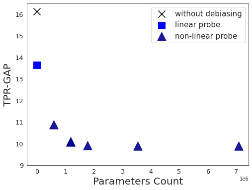
Figure 3: The TPR-GAP results obtained by applying IGBP with different probe classifier architectures on the Bias in Bios dataset.

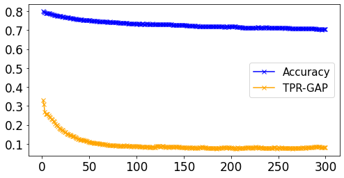
Figure 4: Mean accuracy and TPR-GAP results versus number of iterations on DIAL dataset, averaged over 5 different random seeds.

5.2 Perforamnce – Fairness Tradeoff

One of the key factors that influence the effectiveness of our method is the number of iterations used. Varying the number of iterations and measuring the resulting changes in the TPR-GAP and downstream task accuracy on the DIAL development set shows that the number of iterations had a significant impact on attribute removal in the early stages (Figure 4), but eventually reached a plateau. Increasing the number of iterations also harmed downstream task accuracy, but the decrease was gradual. A similar experiment on Bias in Bios (Appendix E) showed the same trend. The results suggest that the balance between performance and fairness can be controlled by adjusting the number of iterations or by implementing appropriate stopping criteria.

6 Conclusion

We presented a gradient-based method for the erasure of non-linearly encoded concepts in text representations. Its ability to remove non-linear information makes it particularly useful for addressing the complex biases that may be present in text representations learned through complex models. We empirically show the effectiveness of our approach to mitigate social biases in representations, thereby improving fairness in models’ decision-making.

Beyond mitigating bias, the Iterative Gradient-Based Projection method has the potential to be applied in a wide range of other contexts, such as increasing model interpretability by applying causal interventions, adapting models to new domains by removing domain-specific information and ensuring privacy by removing sensitive information. In future work, we plan to explore these and other potential applications of the proposed method.

Limitations

The proposed method has limitations in its dependence on the accuracy and performance of the probe classifier as noted in Belinkov (2022), and may be limited in scenarios where the dataset is small or lacks sufficient information about the protected attribute. Additionally, this approach increases inference time due to the use of a sequential debiasing classifiers. In future work, we aim to find a single probe that eliminates non-linear leakage. Finally, the proposed method aims to eliminate information about a protected attribute in neural representations. While it may align with fairness metrics such as demographic parity, it is not specifically designed to ensure them.

Ethical Considerations

Ethical considerations are of utmost importance in this work. It is essential to exercise caution and consider the ethical implications when using this method, as it has the potential to be applied in situations where fair and unbiased decision-making is critical. It is important to thoroughly evaluate the effectiveness of the method in the specific context in which it will be used, and to carefully consider the data, fairness metrics, and overall application before deploying it. It is worth noting that our method is limited by the fact that gender is a non-binary concept and that it does not address all forms of bias, and further research is necessary to identify and address these biases. Additionally, it is important to consider the potential risk of inadvertently increasing bias through reversing the direction of the debiasing operation in the algorithm. It is crucial to be mindful of the potential impact of this method and to approach its use with caution and care.

Appendix

Appendix A Continuous Attributes

While this work focuses on discrete attribute information-removal, we explain briefly how it can be adapted for regression problems, where the attribute is continuous (e.g., age). In discrete attribute classification tasks, Given that $f$ is the classifier, IGBP is designed to transform each vector $x$ to $x^{\prime}$ onto the decision boundary of $f$ such that $f(x^{\prime})=0$. In the continuous case, where $f$ is the attribute regressor, IGBP aims to achieve a similar result, with the goal of projecting each vector $x$ onto a point $x^{\prime}$ such that $f(x^{\prime})=0$. Hence, each input, x, is regressed to a non-informative value of zero, meaning that the input is stripped of its information content.

Appendix B Reversal Gradient of Cross Entropy

Let us consider a non-linear model $f(x)$ followed by a logistic function to obtain the probabilty $p=\frac{1}{1+e^{f(x)}}$. Then the gradient of $L_{CE}(p_{t})$ when $y=1$ is :

$$\nabla_{x}{L_{CE}}=\frac{\partial L_{CE}}{\partial p_{t}}\frac{\partial p_{t}}{\partial f}\frac{\partial f}{\partial x}\\ \hskip 27.0pt=\frac{-1}{p_{t}}\>p_{t}(1-p_{t})\>\nabla_{x}{f}\\ =-(1-p_{t})\>\nabla_{x}{f}\\$$ (11)

and $\nabla_{x}{L_{CE}}=+(1-p_{t})\>\nabla_{x}{f}$ when $y=-1$.

Appendix C Local Linear Model Projection

We will now show how the projective loss update step projects each sample to its local linear model boundary. This will facilitate the probe being oblivious to the protected attribute.

Local Linearity.

First, we will show that a trained ReLU neural net probe divides the embedding space into sub-regions, where in each sub-region it behaves as a linear model. We will demonstrate that we can obtain the local linear model for each embedding. Let us consider a non-linear probe composed of one-hidden layer with ReLU as an activation function:

$$z=x^{\top}W,\\ h=ReLU(z),\\ f=h^{\top}\theta,\\ p=\frac{1}{1+e^{-f(x)}}\\$$ (12)

The activation function ReLU acts as an element-wise scalar (0 or 1) multiplication, hence h can be written as:

$$h=a\odot z$$ (13)

where $a$ is a vector with (0,1) entries indicating the slopes of ReLU in the corresponding linear regions where z fall into. Let us define a diagonal matrix $D$:

$$D=diag(a)$$ (14)

Then,

$$h=Dz$$ (15)

since doing element wise multiplication with a vector $a$ is the same as multiplication by the diagonal matrix $D$. It is now possible to express the output in each sub-region in matrix form as follows:

$$f=h^{\top}\theta\\ =(DWx)^{\top}\theta\\ =x^{\top}(DW)^{\top}\theta\\$$ (16)

$D$ expresses the ReLU function, so naturally it depends on $Wx$, but since the weights of the probe are frozen/constant and we are doing the calculation for the sub-region where the slope of the ReLU function is constant, we can assume that $D$ is not dependent on $x$ in this sub-region.Thus, in each sub-region $r$ defined by the classifier, the local linear model for this sub-region is $\theta_{r}$ defined bellow :

$$\theta_{r}=(DW)^{\top}\theta\\$$ (17)

We can obtain the vector $\theta_{r}$ with the gradient of $f$:

$$\nabla_{x}{f}=(DW)^{\top}\theta\\$$ (18)

Applying the chain rule with $L_{P}(p_{t})$ as in Eq. LABEL:eq:chain-rule for each sub-region:

$$\nabla_{x}{L_{P}}=\frac{\partial L_{P}}{\partial p_{t}}\frac{\partial p_{t}}{\partial p}\frac{\partial p}{\partial f}\frac{\partial f}{\partial x}\\ =\frac{log(\frac{p_{t}}{1-p_{t}})}{p_{t}(1-p_{t})}(-1)^{y}p(1-p)\nabla_{x}{f}^{\top}\\ =(-1)^{-y}f(x)(-1)^{y}\nabla_{x}{f}^{\top}\\ =f(x)\nabla_{x}{f}^{\top}\quad\\ \hskip 10.00002pt=x^{\top}(DW)^{\top}\theta((DW)^{\top}\theta)^{\top}\text{(Using Eq.~{}\ref{eq:f=x..},\ref{eq:dfdx})}\\ =(x^{\top}\theta_{r})\theta_{r}^{\top}\\$$ (19)

Again, we can obtain $\theta_{r}$ from the gradient and divide the term with $\frac{1}{\theta_{r}^{\top}\theta_{r}}$ to get the linear projection of each sub-region to its linear model null space

$$x_{p}=x-(\frac{x^{\top}\theta_{r}}{\theta_{r}^{\top}\theta_{r}})\theta_{r}^{\top}$$ (20)

Appendix D Experiment

This section provides additional details on the experimental setup and results.

D.1 Implementaion details

IGBP stopping criteria.

In order to balance the trade-off between reducing extrinsic and intrinsic bias while preserving accuracy (as can be seen in Section 5.2), we have established a stopping criterion for our proposed method, IGBP . The criterion is based on two factors: the accuracy of a newly trained probe classifier on the protected attribute, and the main task accuracy on the development set. Specifically, we run Algorithm 1 until the newly trained probe classifier acheives within 2% above-majority accuracy, or until the main task accuracy on the development set drops below a threshold of 0.98 of the original main task accuracy. Through empirical analysis on the development set, we have determined that this threshold yields good results for all extrinsic evaluation experiments. However, it is worth noting that this stopping criterion may be adjusted based on specific requirements for each case.

IGBP classifier type.

For all experiments, we use a a ReLU MLP as the attribute classifier with a single-hidden layer of the same size as the input dimension. We train the classifier with AdamW optimizer Loshchilov and Hutter (2018) with learning rate of $2e^{-4}$ and batch size of 256.
Applying the algorithm for training on DIAL dataset takes about 0.5-1 hour and 1-3 hours on Bias in Bios on NVIDIA GeForce RTX 2080 Ti.

Compeing methods implementation and hyperparameters.

For competing methods, we follow their implementations that can be found here. We run the algorithms until the specific type of leakage they were trying to eliminate was no longer present. For KCE we choose RBF kernel following their selection in their paper for Bias in Bios task. We tried multiple kernels but found that RBF yeilds better results. The results of RLACE are different than those in the original paper because they used only the first 100K of training samples and applied a PCA transformation to reduce dimensions down to 300 due to the high computation time. However, we wanted to make fair comparison so we did not reduce the size of training set or the dimensionality.

Models.

We used the pre-trained BERT and RoBERTa base models by Huggingface that have 110M and 123M parameters. They were fine-tuned on the proffesion prediction task in Bias in Bios using a stochastic gradient descent (SGD) optimizer with a learning rate of $5e^{-4}$, weight decay of $1e^{-6}$, and momentum of $0.90$. We trained for $30,000$ batches of size $10$.

D.2 GloVe Word Embeddings Experiment

We provide details about the experimental settings in the static word vectors experiment 4.3. We follow Ravfogel et al. (2020) and use uncased GloVe word embeddings of 150,000 most common words. We project all vectors on $\vec{he}-\vec{she}$ direction, and select the 7500 most male-biased and female biased words. Using the same training–development–test split as Ravfogel et al. (2020), we subtract the gender-neutral words and end up with a training set of 7350, an evaluation set of 3150, and a test set of 4500.

D.2.1 Additional intrinsic evaluation

We evaluate bias-by-neighbors which was proposed by Gonen and Goldberg (2019) and the list of professions from Bolukbasi et al. (2016). We determine the correlation between bias-by-projection and bias-by-neighbors by calculating the percentage of top 100 neighboring words for each profession that were originally biased-by-projection towards a specific gender. Our results show mean correlation of 0.598, which is lower than the previous correlation of 0.852. In comparison, after applying INLP we find a correlation of 0.73. This suggests that while some bias-by-neighbors still remains, the debiasing effect of IGBP is significant.

D.2.2 Nearest Neighbors

We demonstrated in Section 4.3.3 that debiasing using IGBP did not cause significant harm to the GloVe word embedding space as per the SimLex999 test results. To further support this, in Table 7, we present the closest neighbors to 10 randomly sampled words from the vocabulary, both before and after our debiasing procedure, as a qualitative illustration.

Word	Neighbors Before	Neighbors After
period	periods,during,time	periods,during,time
actual	exact,any,same	exact,any,same
markers	marker,marking,pens	marker,marking,pens
photoshop	adobe,illustrator,indesign	adobe,illustrator,indesign
commands	command,execute,instructions	command,execute,scripts
adapted	adaptation,adapting,adapt	adaptation,adapting,adapt
called	known,which,that	known,which,also
vital	crucial,important,essential	crucial,important,essential
heritage	cultural,historic,historical	cultural, historic,historical
mood	moods,feeling,feel	moods,feeling,feel

Table 7: 3-neighbors of random words in GloVe embedding space before and after IGBP debiasing.

D.3 Extrinsic Evaluation Experiments

D.3.1 Metrics

We provide additional details on the metrics used in Section 4.4

Main task model.

We use sklearn’s SVM Pedregosa et al. (2011) for the main task predictions on DIAL experiment, and sklearn’s logistic regression for Bias in Bios which is a multi-label classification task.

Leakage and MDL Compression.

MDL is an information-theoretic probing which measures how efficiently a model can extract information about the labels from the inputs . In this work, we employ the online coding approach Voita and Titov (2020) to calculate MDL. We estimate MDL following Voita and Titov’s online coding $L_{online}$ and calcuate the compression, C, which is compared against uniform encoding $L_{uniform}$ which does not require any learning from data.

$$C=\frac{L_{uniform}}{L_{online}}$$

We evaluate our models using an online code probe, which is trained on fractions of the training dataset: [2.0, 3.0, 4.4, 6.5, 9.5, 14.0, 21.0, 31.0, 45.7, 67.6, 100]. Then we calculate leakage as the probe’s accuracy on test set when trained on the entire training set. We use a MLP with two-hidden layer of size 512 and ReLU activation as the probe classifier. This decision was made to stay consistent with previous work which employed MDL Mendelson and Belinkov (2021) and to have a different and more powerful adversary than the one used in IGBP .

Appendix E Analysis

E.1 Biographies representation

We present the t-SNE Van der Maaten and Hinton (2008) projections of the biographies representations of BERT before and after applying IGBP.

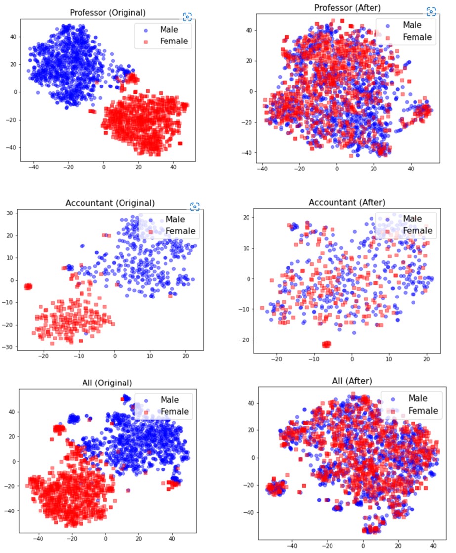
Figure 5: The t-SNE projections of BERT representations for various professions, including Professors, Accountants, and all proffesions, before and after applying IGBP.

E.2 Benefits of Non-Linear Information Removal

We present the probe architectures we use in our expirement Section 5.1. These include a linear probe with one layer, and several non-linear probes that use ReLU activations. From left to right: one-hidden layer of the same size as the input dimension, two-hidden layers with the same size as the input dimension, one-hidden layer with size of twice the input dimension, three-hidden layers with size of input dimension, one-hidden layer with size of three times the input dimension. Figure 6 shows the results of Section 5.1 experiment on DIAL dataset. We observe the same trend. The maximum accuracy drop is 1.32%.

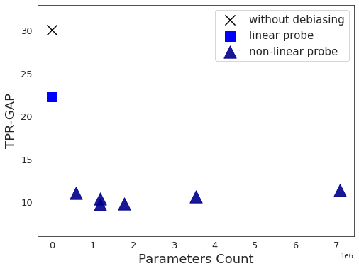
Figure 6: The TPR-GAP results obtained by applying IGBP with different probe classifier architectures on the DIAL dataset.

E.2.1 Number of Iterations

We conduct the same experiment of Section 5.2 on DIAL dataset and show the result in Figure 7.

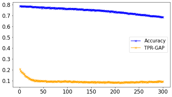
Figure 7: Mean accuracy and TPR-GAP results versus number of iterations on Bias in Bios dataset with Bert as encoder, averaged over 5 different random seeds.

References

- Belinkov (2022) Yonatan Belinkov. 2022. Probing classifiers: Promises, shortcomings, and advances. Computational Linguistics, 48(1):207–219.
- Beutel et al. (2017) Alex Beutel, Jilin Chen, Zhe Zhao, and Ed H. Chi. 2017. Data decisions and theoretical implications when adversarially learning fair representations. CoRR, abs/1707.00075.
- Blodgett et al. (2016) Su Lin Blodgett, Lisa Green, and Brendan O’Connor. 2016. Demographic dialectal variation in social media: A case study of African-American English. In Proceedings of the 2016 Conference on Empirical Methods in Natural Language Processing, pages 1119–1130, Austin, Texas. Association for Computational Linguistics.
- Bolukbasi et al. (2016) Tolga Bolukbasi, Kai-Wei Chang, James Y Zou, Venkatesh Saligrama, and Adam T Kalai. 2016. Man is to computer programmer as woman is to homemaker? debiasing word embeddings. Advances in neural information processing systems, 29.
- Caliskan et al. (2017) Aylin Caliskan, Joanna J Bryson, and Arvind Narayanan. 2017. Semantics derived automatically from language corpora contain human-like biases. Science, 356(6334):183–186.
- De-Arteaga et al. (2019) Maria De-Arteaga, Alexey Romanov, Hanna Wallach, Jennifer Chayes, Christian Borgs, Alexandra Chouldechova, Sahin Geyik, Krishnaram Kenthapadi, and Adam Tauman Kalai. 2019. Bias in bios: A case study of semantic representation bias in a high-stakes setting. In Proceedings of the Conference on Fairness, Accountability, and Transparency, FAT* ’19, page 120–128, New York, NY, USA. Association for Computing Machinery.
- Devlin et al. (2019) Jacob Devlin, Ming-Wei Chang, Kenton Lee, and Kristina Toutanova. 2019. BERT: pre-training of deep bidirectional transformers for language understanding. In Proceedings of the 2019 Conference of the North American Chapter of the Association for Computational Linguistics: Human Language Technologies, NAACL-HLT 2019, Minneapolis, MN, USA, June 2-7, 2019, Volume 1 (Long and Short Papers), pages 4171–4186. Association for Computational Linguistics.
- Elazar and Goldberg (2018) Yanai Elazar and Yoav Goldberg. 2018. Adversarial removal of demographic attributes from text data. In Proceedings of the 2018 Conference on Empirical Methods in Natural Language Processing, Brussels, Belgium, October 31 - November 4, 2018, pages 11–21. Association for Computational Linguistics.
- Felbo et al. (2017) Bjarke Felbo, Alan Mislove, Anders Søgaard, Iyad Rahwan, and Sune Lehmann. 2017. Using millions of emoji occurrences to learn any-domain representations for detecting sentiment, emotion and sarcasm. In Conference on Empirical Methods in Natural Language Processing (EMNLP).
- Gonen and Goldberg (2019) Hila Gonen and Yoav Goldberg. 2019. Lipstick on a pig: Debiasing methods cover up systematic gender biases in word embeddings but do not remove them. In Proceedings of the 2019 Workshop on Widening NLP@ACL 2019, Florence, Italy, July 28, 2019, pages 60–63. Association for Computational Linguistics.
- Hill et al. (2015) Felix Hill, Roi Reichart, and Anna Korhonen. 2015. Simlex-999: Evaluating semantic models with (genuine) similarity estimation. Computational Linguistics, 41(4):665–695.
- Kumar et al. (2022) Abhinav Kumar, Chenhao Tan, and Amit Sharma. 2022. Probing classifiers are unreliable for concept removal and detection. In ICML 2022: Workshop on Spurious Correlations, Invariance and Stability.
- Liu et al. (2019) Yinhan Liu, Myle Ott, Naman Goyal, Jingfei Du, Mandar Joshi, Danqi Chen, Omer Levy, Mike Lewis, Luke Zettlemoyer, and Veselin Stoyanov. 2019. Roberta: A robustly optimized BERT pretraining approach. CoRR, abs/1907.11692.
- Loshchilov and Hutter (2018) Ilya Loshchilov and Frank Hutter. 2018. Decoupled weight decay regularization. In International Conference on Learning Representations.
- Mendelson and Belinkov (2021) Michael Mendelson and Yonatan Belinkov. 2021. Debiasing methods in natural language understanding make bias more accessible. In Proceedings of the 2021 Conference on Empirical Methods in Natural Language Processing, pages 1545–1557, Online and Punta Cana, Dominican Republic. Association for Computational Linguistics.
- Orgad and Belinkov (2022) Hadas Orgad and Yonatan Belinkov. 2022. Choose your lenses: Flaws in gender bias evaluation. In Proceedings of the 4th Workshop on Gender Bias in Natural Language Processing (GeBNLP), pages 151–167, Seattle, Washington. Association for Computational Linguistics.
- Orgad and Belinkov (2023) Hadas Orgad and Yonatan Belinkov. 2023. Debiasing NLP models without demographic information. In Proceedings of the 61th Annual Meeting of the Association for Computational Linguistics, ACL 2023, July 9-14, 2023. Association for Computational Linguistics.
- Orgad et al. (2022) Hadas Orgad, Seraphina Goldfarb-Tarrant, and Yonatan Belinkov. 2022. How gender debiasing affects internal model representations, and why it matters. In Proceedings of the 2022 Conference of the North American Chapter of the Association for Computational Linguistics: Human Language Technologies, pages 2602–2628, Seattle, United States. Association for Computational Linguistics.
- Pedregosa et al. (2011) F. Pedregosa, G. Varoquaux, A. Gramfort, V. Michel, B. Thirion, O. Grisel, M. Blondel, P. Prettenhofer, R. Weiss, V. Dubourg, J. Vanderplas, A. Passos, D. Cournapeau, M. Brucher, M. Perrot, and E. Duchesnay. 2011. Scikit-learn: Machine learning in Python. Journal of Machine Learning Research, 12:2825–2830.
- Pennington et al. (2014) Jeffrey Pennington, Richard Socher, and Christopher Manning. 2014. GloVe: Global vectors for word representation. In Proceedings of the 2014 Conference on Empirical Methods in Natural Language Processing (EMNLP), pages 1532–1543, Doha, Qatar. Association for Computational Linguistics.
- Ravfogel et al. (2020) Shauli Ravfogel, Yanai Elazar, Hila Gonen, Michael Twiton, and Yoav Goldberg. 2020. Null it out: Guarding protected attributes by iterative nullspace projection. In Proceedings of the 58th Annual Meeting of the Association for Computational Linguistics, ACL 2020, Online, July 5-10, 2020, pages 7237–7256. Association for Computational Linguistics.
- Ravfogel et al. (2022a) Shauli Ravfogel, Michael Twiton, Yoav Goldberg, and Ryan Cotterell. 2022a. Linear adversarial concept erasure. In International Conference on Machine Learning, ICML 2022, 17-23 July 2022, Baltimore, Maryland, USA, volume 162 of Proceedings of Machine Learning Research, pages 18400–18421. PMLR.
- Ravfogel et al. (2022b) Shauli Ravfogel, Francisco Vargas, Yoav Goldberg, and Ryan Cotterell. 2022b. Adversarial concept erasure in kernel space. In Proceedings of the 2022 Conference on Empirical Methods in Natural Language Processing, pages 6034–6055, Abu Dhabi, United Arab Emirates. Association for Computational Linguistics.
- Romanov et al. (2019) Alexey Romanov, Maria De-Arteaga, Hanna Wallach, Jennifer Chayes, Christian Borgs, Alexandra Chouldechova, Sahin Geyik, Krishnaram Kenthapadi, Anna Rumshisky, and Adam Kalai. 2019. What’s in a name? Reducing bias in bios without access to protected attributes. In Proceedings of the 2019 Conference of the North American Chapter of the Association for Computational Linguistics: Human Language Technologies, Volume 1 (Long and Short Papers), pages 4187–4195, Minneapolis, Minnesota. Association for Computational Linguistics.
- Rudinger et al. (2018) Rachel Rudinger, Jason Naradowsky, Brian Leonard, and Benjamin Van Durme. 2018. Gender bias in coreference resolution. In Proceedings of the 2018 Conference of the North American Chapter of the Association for Computational Linguistics: Human Language Technologies, NAACL-HLT, New Orleans, Louisiana, USA, June 1-6, 2018, Volume 2 (Short Papers), pages 8–14. Association for Computational Linguistics.
- Shao et al. (2023) Shun Shao, Yftah Ziser, and Shay B. Cohen. 2023. Gold doesn’t always glitter: Spectral removal of linear and nonlinear guarded attribute information. In Proceedings of the 17th Conference of the European Chapter of the Association for Computational Linguistics, pages 1611–1622, Dubrovnik, Croatia. Association for Computational Linguistics.
- Van der Maaten and Hinton (2008) Laurens Van der Maaten and Geoffrey Hinton. 2008. Visualizing data using t-sne. Journal of machine learning research, 9(11).
- Voita and Titov (2020) Elena Voita and Ivan Titov. 2020. Information-theoretic probing with minimum description length. In Proceedings of the 2020 Conference on Empirical Methods in Natural Language Processing (EMNLP), pages 183–196, Online. Association for Computational Linguistics.
- Wang et al. (2020) Tianlu Wang, Xi Victoria Lin, Nazneen Fatema Rajani, Bryan McCann, Vicente Ordonez, and Caiming Xiong. 2020. Double-hard debias: Tailoring word embeddings for gender bias mitigation. In Proceedings of the 58th Annual Meeting of the Association for Computational Linguistics, pages 5443–5453, Online. Association for Computational Linguistics.
- Wang et al. (2019) Tianlu Wang, Jieyu Zhao, Mark Yatskar, Kai-Wei Chang, and Vicente Ordonez. 2019. Balanced datasets are not enough: Estimating and mitigating gender bias in deep image representations. In 2019 IEEE/CVF International Conference on Computer Vision, ICCV 2019, Seoul, Korea (South), October 27 - November 2, 2019, pages 5309–5318. IEEE.
- Xie et al. (2017) Qizhe Xie, Zihang Dai, Yulun Du, Eduard Hovy, and Graham Neubig. 2017. Controllable invariance through adversarial feature learning. Advances in neural information processing systems, 30.
- Zhang et al. (2018) Brian Hu Zhang, Blake Lemoine, and Margaret Mitchell. 2018. Mitigating unwanted biases with adversarial learning. In Proceedings of the 2018 AAAI/ACM Conference on AI, Ethics, and Society, pages 335–340.
- Zhao et al. (2018) Jieyu Zhao, Tianlu Wang, Mark Yatskar, Vicente Ordonez, and Kai-Wei Chang. 2018. Gender bias in coreference resolution: Evaluation and debiasing methods. In Proceedings of the 2018 Conference of the North American Chapter of the Association for Computational Linguistics: Human Language Technologies, NAACL-HLT, New Orleans, Louisiana, USA, June 1-6, 2018, Volume 2 (Short Papers), pages 15–20. Association for Computational Linguistics.