IDO-VFI: Identifying Dynamics via Optical Flow Guidance for Video Frame Interpolation with Events

Abstract

Video frame interpolation aims to generate high-quality intermediate frames from boundary frames and increase frame rate. While existing linear, symmetric and nonlinear models are used to bridge the gap from the lack of inter-frame motion, they cannot reconstruct real motions. Event cameras, however, are ideal for capturing inter-frame dynamics with their extremely high temporal resolution. In this paper, we propose an event-and-frame-based video frame interpolation method named IDO-VFI that assigns varying amounts of computation for different sub-regions via optical flow guidance. The proposed method first estimates the optical flow based on frames and events, and then decides whether to further calculate the residual optical flow in those sub-regions via a Gumbel gating module according to the optical flow amplitude. Intermediate frames are eventually generated through a concise Transformer-based fusion network. Our proposed method maintains high-quality performance while reducing computation time and computational effort by 10% and 17% respectively on Vimeo90K datasets, compared with a unified process on the whole region. Moreover, our method outperforms state-of-the-art frame-only and frames-plus-events methods on multiple video frame interpolation benchmarks. Codes and models are available at https://github.com/shicy17/IDO-VFI.

1 Introduction

Video frame interpolation (VFI) increases the video frame rate by inserting a reconstruction frame into two consecutive frames. Due to the limitation of the fixed frame rate of ordinary camera, the frame-only video frame interpolation methods inevitably lose the dynamics in the interval between consecutive frames. In order to compensate for the lack of inter-frame information, motion models are often used, but those models cannot account for the real motions.

Event cameras posch2014retinomorphic are bio-inspired vision sensor, each pixel of which independently perceives and encodes relative changes in light intensity. Event cameras output sparse, asynchronous streams of events instead of frames, with advantages of high temporal resolution, high dynamics, and low power consumption. An event is usually expressed as a tuple $e=(x,y,p,t)$, which means that at timestamp $t$, an event with polarity $p\in\{-1,1\}$ is generated at the pixel $(x,y)$. Positive polarity indicates that the change of light intensity from week to strong is beyond the threshold, while negative polarity is just the opposite. Because an event camera has high temporal resolution up to microseconds, it can capture complete changes or motion between frames.

The event flow is the embodiment of inter-frame changes. Therefore, the optical flow estimated from the events does not require any motion model to be fitted, which can be inherently nonlinear. Since events lack intensity information, frame-based optical flow is complementary to event-based optical flow. By combining these two kinds of optical flow, more accurate estimation results can be obtained. Meanwhile, it is possible to reconstruct high-quality keyframes at any timestamp, since real inter-frame dynamics are captured.

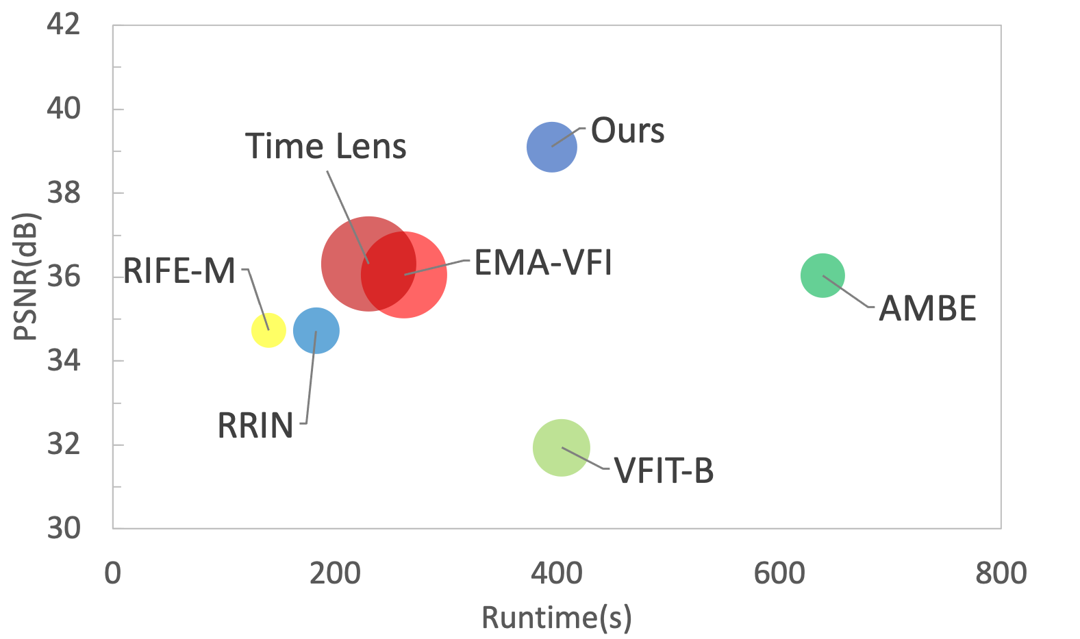
(a) PSNR/Runtime/Parameters comparison

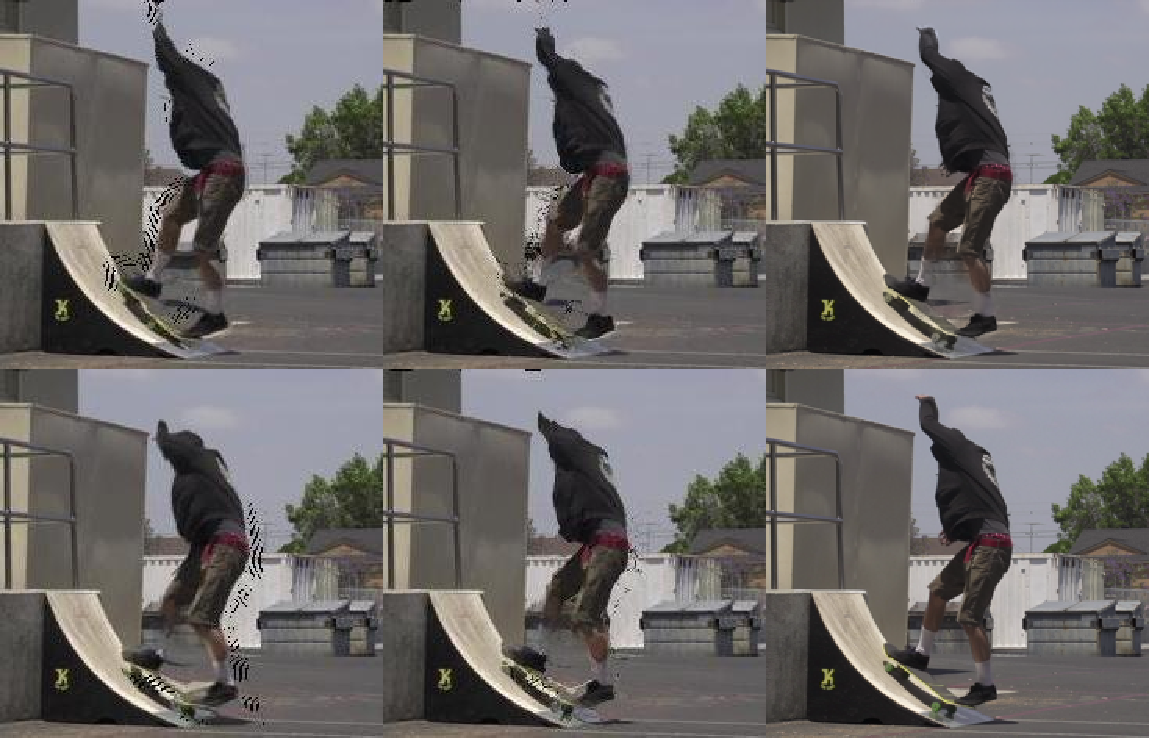
(b) Results of proposed each module on Vimeo90K

Figure 1: (a) The quantitative PSNR/Runtime/Parameters comparison of ours and state-of-the-art VFI methods on Vimeo90K. The larger circle represents larger number of parameters. Our proposed method achieves the best performance with relatively small model parameters and fast computation time. (b) Results of proposed each module on Vimeo90K. The first column shows the warping-based results of optical flow estimation module. The second column presents refined frames generated from residual flow estimation module. Right top is the final output, and right bottom is the ground-truth. The quality of output improves step by step.

Furthermore, the real inter-frame motion information lays the foundation for reliable differential processing of different image regions. For pixel areas with small motion amplitudes, only a simple estimation is needed to obtain an accurate optical flow field. However, for complex dynamic regions where simple optical flow estimation is insufficient to address the problem, further estimation of residual optical flow is required in order to obtain more accurate results. With the help of event flow, we can easily distinguish dynamic and static areas in the image, and adopt different optical flow estimation strategies, which can greatly reduce the amount of calculation while maintaining high-precision results. Our main contributions are as follows:

• A novel and trainable optical flow guidance mechanism for identifying the dynamics of the boundary frames and events is proposed, considering the corresponding relationship between adjacent dynamic regions.

• We propose an event-based residual optical flow estimation method to further dynamically evaluate the optical flow field, of which the computation time and computational effort are reduced by 10% and 17% respectively, while the performance is almost the same as processing the whole image without distinction.

• Our proposed method achieves state-of-the-art results on multiple benchmark datasets compared to frame-only and events-plus-frames VFI methods. Codes and models are available publicly.

This paper is organized as follows. First, the main work in this field is introduced. Second, our proposed VFI method and its components are present. Third, the experimental details and quantitative results are illustrated. Subsequently, ablation experiments are conducted. Finally, the paper is summarized and discussed.

(a) Ground Truth

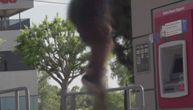
(b) RIFE

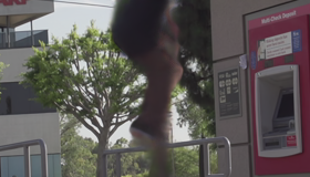
(c) AMBE

(d) EMA-VFI

(e) Ours

Figure 2: Visual comparison among our proposed method, the state-of-the-art methods RIFE, AMBE, EMA-VFI on the Vimeo90K-triplet validation set.

2 Related Works

Reconstructing dynamics and luminosity is the key task of VFI. Thus, the warping-based methods and synthesis-based methods become the mainstream methods of VFI.

Frame-only VFI Methods. Warping-based methods use photometric consistency assumptions to estimate inter-frame motion, which is very effective for video sequences with short inter-frame blind times and simple motion, but it only warps pixels and cannot reconstruct photometric information. The original methods usually assume that the optical flow between frames is first-order, such as sun2018pwc ; jiang2018super ; bao2019depth ; park2020bmbc ; niklaus2020softmax ; sim2021xvfi ; yu2022deep .Meanwhile, several complex motion models have been proposed. Xu et al.xu2019quadratic proposed a method for estimating the secondary optical flow, but this method needs to input four key frames at a time. Park et al. proposed AMBE park2021asymmetric , on the basis of BMBC park2020bmbc , using anchor frames to estimate asymmetric motion without relying on linear optical flow assumptions. However, the assumed motion models may fail once the actual motion becomes complex.

Synthesis-based methods lee2020adacof ; choi2021motion ; shi2022video ; niklaus2023splatting directly fuses the image features of boundary frames to generate intermediate frames, which can reconstruct photometric information. However, the synthesis method performs poorly when there is complex motion in the time interval. In order to restore this defect, it usually takes multiple consecutive frames, e.g. four frames shi2022video , as input. Some models shangguan2022learning ; oh2022demfi combine warping-based and synthesis-based methods, considering complementarity between the two, which can reconstruct dynamics and photometry while estimating inter-frame motion.

Events-plus-frames VFI Methods. In recent years, there have been attempts pan2019bringing ; wang2020joint ; yu2021training ; tulyakov2021time ; tulyakov2022time ; he2022timereplayer ; zhang2022unifying ; wu2022video to combine frames and events for VFI. Event-based optical flow can still be accurately estimated under condition of complex intermediate motions, since event-based optical flow estimation is not based on linearity assumptions. Although event cameras do not encode photometric information, they are complementary to frame-based cameras. Yu et al. yu2021training respectively extracted the multi-scale features of events and frames for fusion, and proposed a sub-pixel-level attention mechanism, which uses event information to supplement inter-frame information to achieve weakly supervised learning. Tulyakov et al. tulyakov2021time proposed Time Lens, which combines events and frames to generate warping-based and synthesis-based images respectively, and outputs the final result through an attention-based network. However, it has a very large number of model parameters. On the ground of tulyakov2021time , Tulyakov et al. proposed Time Lens++ tulyakov2022time , which encodes optical flow as cubic splines and warps the features for fusion in an encoder-decoder network. Unfortunately, the amount of model parameters is still large. He et al. proposed TimeReplayer he2022timereplayer , an event-based unsupervised video frame interpolation method. The unsupervised learning method decreases the dependency on the use of high frame-rate datasets. Although these methods achieve good performance, they are computationally expensive and do not maximize the advantages of the properties of events to characterize motion.

Combining events and frames can estimate the complete inter-frame motion without any motion model, so the motion amplitude of all pixel regions can be obtained. Simple processing is enough for areas with small motion amplitude. Only areas with large motion amplitude require more complex processing. Therefore adopting different calculation strategies for pixel regions with different motion amplitude can save calculation, while maintaining the quality of the output. Some frame-only VFI methods for reducing the computational overhead have been proposed. Choi et al. choi2021motion proposed a method to evaluate the motion of the local area, reasonably select the model depth to process the local area, or perform downscale processing on the local area at different scales, so as to reduce the computational overhead. But this method is only based on the assumption of photometric consistency and cannot cover complex motions. Therefore, we propose an event-based VFI method that reduces computation time and overhead by dynamically estimating residual optical flow in pixel regions while maintaining high-quality output.

3 Proposed Method

3.1 Problem Formulation

Assuming that we are given two consecutive frames $I_{0}$ and $I_{1}$ at time 0 and 1, as well as events sequences $E_{0\rightarrow 1}$ consisting all events triggered between the interval. The task is generating intermediate frame $\hat{I_{t}}$ at arbitrary time $t$, where $t\in[0,1]$. Besides, according to the interpolating timestamp $t$, we can divide the event sequences $E_{0\rightarrow 1}$ into two parts $E_{0\rightarrow t}$ and $E_{t\rightarrow 1}$. The event sequence $E_{a\rightarrow b}$ is represented as a voxel grid $V_{a\rightarrow b}$ zihao2018unsupervised .

3.2 Overview

The proposed framework is mainly consisted of four components: Optical flow estimation module, Gumbel gating module, Residual optical flow estimation module and Transformer-based fusion module.

First, the existing consecutive frames $I_{0}$, $I_{1}$ and event sequence are input to the optical flow estimation network for calculating bidirectional optical flows $F_{0\rightarrow t}$ and $F_{1\rightarrow t}$. The $I_{0}$ and $I_{1}$ are warped according to these optical flows to generate intermediate frames $I^{warp}_{0}$ and $I^{warp}_{1}$. Subsequently, the boundary frames are evenly divided into multiple sub-regions, which are further categorized as dynamic or static regions according to the Gumbel gating network. The dynamic regions in the image will be fed into the residual optical flow estimation network to estimate the residual optical flows. Then warping the $I^{warp}_{0}$ and $I^{warp}_{1}$ to generate $I_{0\rightarrow t}^{refine}$ and $I_{1\rightarrow t}^{refine}$. The final output of the proposed model is generated by synthesizing the boundary frames and warping-based frames. Unnecessary computing costs of static region could be significantly reduced through this method, while maintaining high-quality final result of the network. The overall architecture is illustrated in Figure.3.

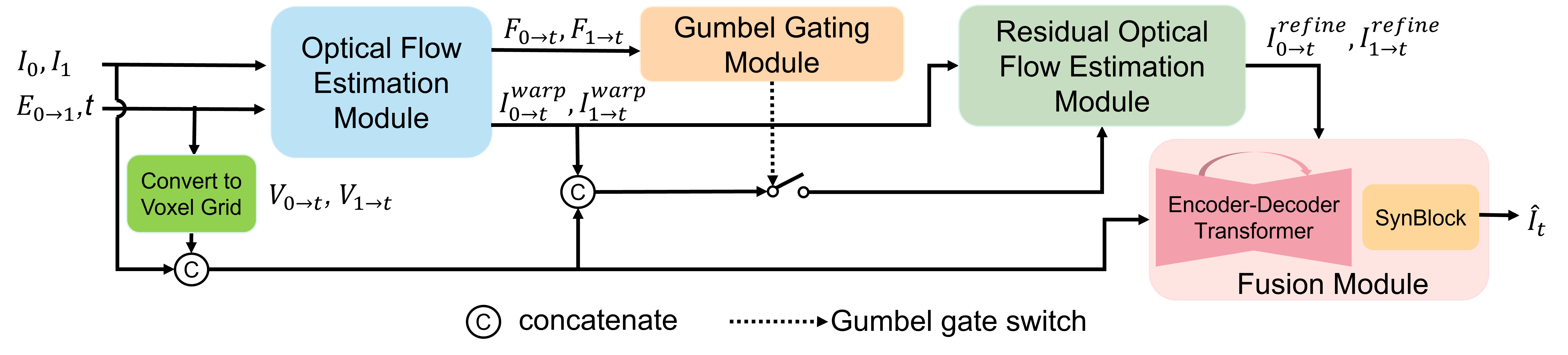
Figure 3: Overview of proposed model architecture.

3.3 Optical Flow Estimation

A UNet jiang2018super is adopted as the backbone of optical flow estimation network, and extended by us for event sequence inputting. Note that the network performs symmetric processing for calculating $F_{0\rightarrow t}$ and $F_{1\rightarrow t}$, we thus only introduce the processing for calculating $F_{0\rightarrow t}$. The flow network extracts feature representations from both input frames $I_{0}$, $I_{1}$ and events $V_{0\rightarrow 1}$. In addition, inspired by Time Lens++tulyakov2022time , we compute cubic motion splines $\{S_{0\rightarrow 1}^{\Delta x},S_{0\rightarrow 1}^{\Delta y}\}$ for each location instead of linear optical flow. These cubic splines which are presented by K-th control points in order to model horizontal and vertical displacement of each pixel of previous frame as a function of time.

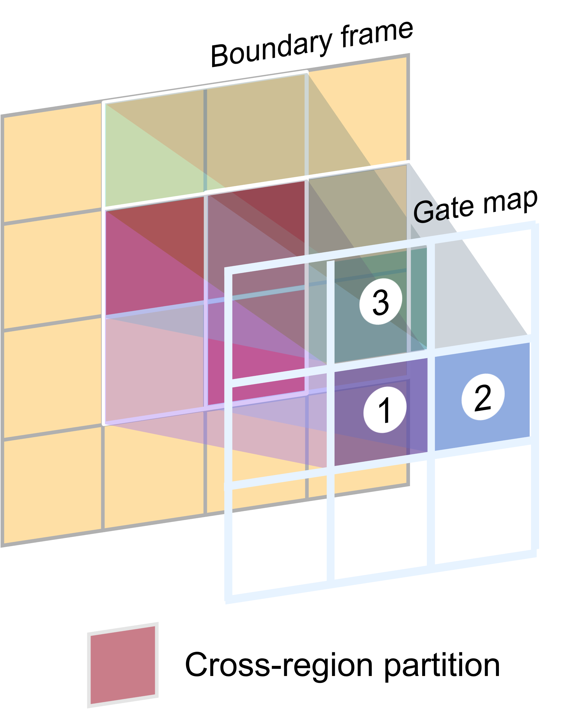
(a) Region division

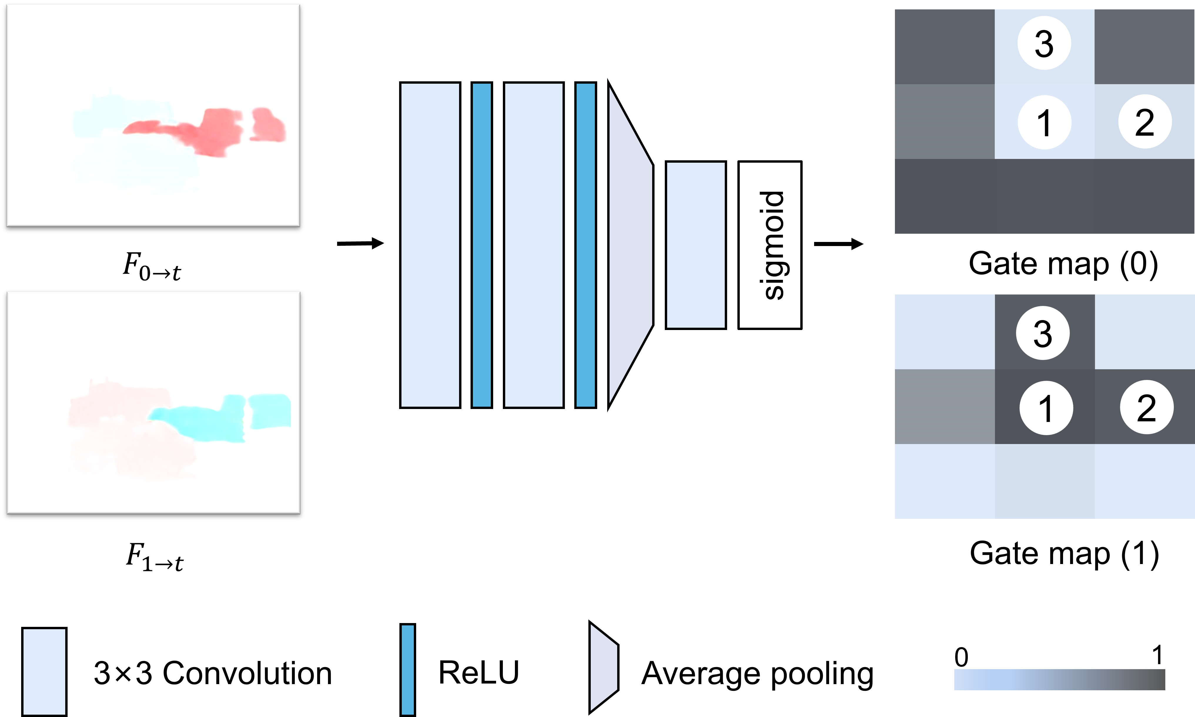
(b) Gating network

Figure 4: The proposed Gumbel gating module.

Optical flows could be obtained by sampling from the motion splines, which reduce the computation cost from $\mathcal{O}(N)$ to $\mathcal{O}(1)$ for the calculation of optical flows. By adding the information of events from blind time, the real motion can be modeled in the flow network. As a result, a nonlinear optical flow $F_{0\rightarrow t}$ for random time $t$ is obtained by sampling from the motion spline $F_{0\rightarrow 1}$ with minimal additional computational cost.

Meanwhile, the intermediate frames $I^{warp}$ are obtained by warping the boundary frames using the estimated optical flow, and described as

$$I_{0}^{warp}=W_{f}(I_{0},F_{0\rightarrow t})$$ (1)

$$I_{1}^{warp}=W_{f}(I_{1},F_{1\rightarrow t})$$ (2)

where $W_{f}(\cdot)$ is the softmax-splatting forward warping operation niklaus2020softmax . Note that, since the estimated optical flow is forward, this forward warping operation is employed.

3.4 Gumbel Gating Module

On the basis of roughly estimating the bilateral optical flow $F_{0\rightarrow t}$ and $F_{1\rightarrow t}$, we then divide the dynamic and static regions in boundary frames. The discrimination of the region type is performed by calculating a Bernoulli probability distribution generated from a trainable Gumbel gating mechanism.

Pixel regions with high-magnitude optical flow field or violent motion will be considered as dynamic regions, and conversely, regions with slight optical flow changes or smooth motion will be considered as static regions. If the whole image is divided into dynamic and static regions according to the optical flow of each pixel, a large number of discrete and irregularly shaped pixel blocks will inevitably appear, which is difficult for further processing. In order to simplify the process, we first set an adjustable rectangular sliding window whose length and width are set to W/2 and H/2 of the input optical flow field respectively. This box will start scanning from the upper left corner of the input, and the horizontal and vertical stride are W/4 and H/4, individually.

As a result, the sliding window operation generates a total of nine pixel regions $R^{0,1}_{i},i=0,1,\cdots,8$ for each boundary frame, and adjacent pixel regions have a cross-region partition, as shown in Figure.4(a). The number of these pixel areas is adjustable. Note that we differ from Choi et al. choi2021motion in that we take into account the connections between adjacent pixel regions. It divides the image into several regions evenly, and the network determines the number of layers that each region needs to process. In contrast, our proposed method preserves the correlation between sub-graphs.

Subsequently, optical flow $F_{0\rightarrow t}$ and $F_{1\rightarrow t}$ are input into a lightweight gating network to generate a gate map $M_{2\times 3\times 3}$. Each pixel on the gate map is a Bernoulli distribution, representing the probability that the corresponding sub-region belongs to the dynamic region or the static region. We can get a binary mask $P$ by rounding the gate map.

$$P=G(M_{2\times 3\times 3})$$ (3)

Where G($\cdot$) is rounding operation, but when training, G($\cdot$) is Gumbel-softmax operation jang2017categorical . The Gumbel-softmax tricks solve the problem that binarization is not differentiable. Note that the final decision is based on the binary mask $P$. The structure of the gating network is shown in Figure.4(b).

3.5 Residual Optical Flow Estimation

All the dynamic regions judged by the Gumbel gating network will be fed into the residual optical flow estimation module to further estimate the residual optical flow.

For a dynamic region $R_{i}^{single},i=0,1,2,\cdots,n$, its corresponding optical flow field $F_{i}^{single}$ and the corresponding parts of $I_{0},I_{1},V_{0\rightarrow t},V_{1\rightarrow t},I_{0}^{warp}$ and $I_{1}^{warp}$ are first concatenated and input into the residual optical flow estimation network. Subsequently, the network will output sub-region refined optical flows $F_{i,1\rightarrow t}^{refine}$ and $F_{i,0\rightarrow t}^{refine}$. Secondly, the refined optical flow of each dynamic region will be padded with 0 to the same size as the boundary frame. They will be fed into an attention-based network to generate a weight map, which is used to calculate the optical flow field coefficient of the corresponding part in each dynamic region that produces the cross-region partition. Thirdly, the residual optical flows in these partitions will be montaged with that of other dynamic regions, and the entire refined optical flows $F^{refine}_{0\rightarrow t}$ and $F^{refine}_{1\rightarrow t}$ will be output. Finally, $I_{0}^{warp}$ and $I_{1}^{warp}$ are processed by backward warping $W_{b}(\cdot)$, and output $I_{0\rightarrow t}^{refine}$ and $I_{1\rightarrow t}^{refine}$, described as follows.

$$I_{0\rightarrow t}^{refine}=W_{b}(I_{0}^{warp},F_{0\rightarrow t})$$ (4)

$$I_{1\rightarrow t}^{refine}=W_{b}(I_{1}^{warp},F_{1\rightarrow t})$$ (5)

Note that backward warping is used to save computation time. Both the residual optical flow estimation network and the attention network are constructed by a UNet, and the entire architecture of residual optical flow estimation module is shown in Figure.5.

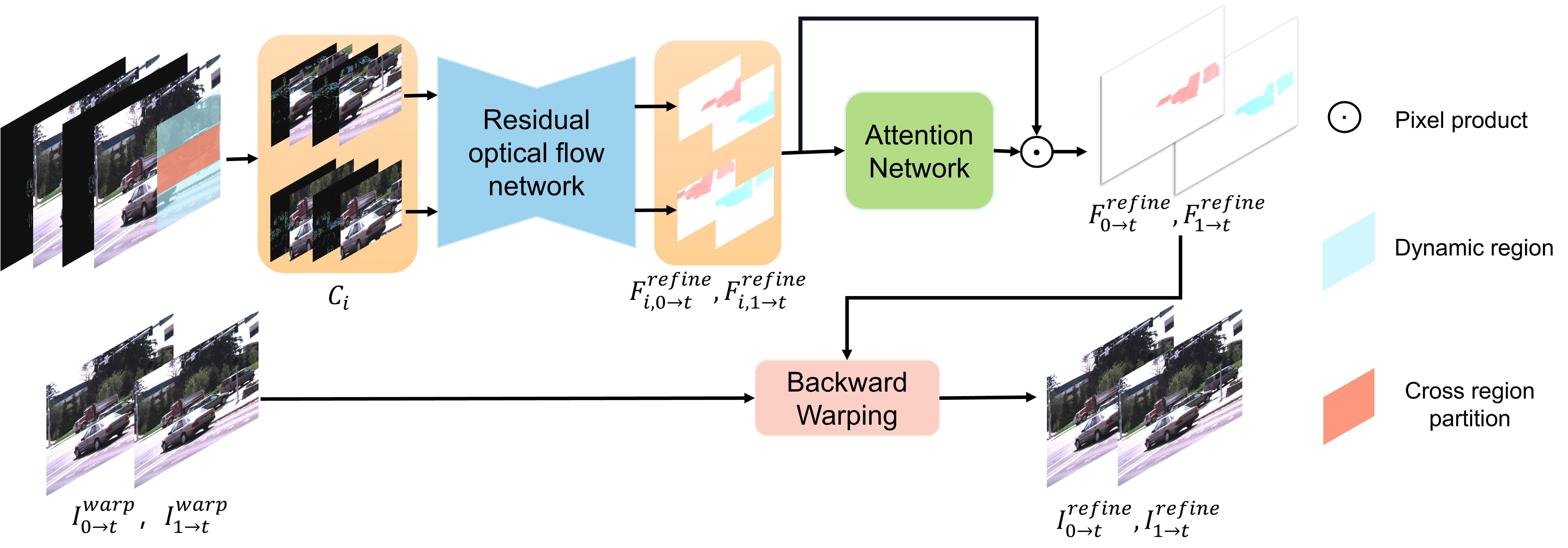
Figure 5: The proposed residual optical flow estimation network.

3.6 Transformer-Based Fusion

The boundary frames $I_{0}$, $I_{1}$, event streams $E_{0\rightarrow t}$, $E_{1\rightarrow t}$, and the warping-based frames $I_{0\rightarrow t}^{refine}$, $I_{1\rightarrow t}^{refine}$ are fed into a Transformer-based encoder-decoder network. This synthesis-based network is modified from VFIT-Bshi2022video . Note that the differences between our method and VFIT-B. First, we only use one SynBlock for fusion. While VFIT-B applies three SynBlocks to achieve feature fusion on three scales. Furthermore, the input for VFIT-B are four consecutive keyframes $I_{0}$, $I_{1}$, $I_{2}$, $I_{3}$. Moreover, VFIT-B only generates one intermediate frame at $t_{0.5}$, while our proposed method can generate intermediate frames at any timestamp. Fortunately, with the help of $I_{0\rightarrow t}^{refine}$, $I_{1\rightarrow t}^{refine}$, we generate results that outperform other methods with a concise fusion network. The output of the block is the final result $I_{t}$, and described as follows.

$$I_{t}=S(I_{0},I_{1},E_{0\rightarrow t},E_{1\rightarrow t},I_{0\rightarrow t}^{refine},I_{1\rightarrow t}^{refine})$$ (6)

where S($\cdot$) is fusion operation.

Table 1: Quantitative comparison of the proposed method with the state-of-the-art methods on multiple VFI benchmarks. Vimeo-3f and Vimeo-7f indicate Vimeo90K-Triplet-Train dataset and Vimeo90K-Septuplet-Train dataset respectively. The best PSNR(dB)\SSIM result is boldfaced, and the second best is underlined. $\ddagger$ indicates that we quote the results in corresponding papers.

Method	Year	Training dataset	Frame	Event	Vimeo90K- Triplet-Test xue2019video		Middleburry baker2011database				GoPronah2017deep				#Param. (Million)
					1 frame skip		1 frame skip		3 frames skip		7 frames skip		15 frames skip
					PSNR	SSIM	PSNR	SSIM	PSNR	SSIM	PSNR	SSIM	PSNR	SSIM
E2VID rebecq2019events	2019	MS-COCO	✗	✓	10.77	0.361	11.51	0.377	11.39	0.375	11.8	0.482	12.11	0.472	10.71
DAIN bao2019depth	2019	Vimeo-3f	✓	✗	34.20	0.962	30.87	0.899	26.67	0.838	28.81	0.876	24.39	0.736	24.03
RRIN li2020video	2020	Vimeo-3f	✓	✗	34.72	0.962	31.08	0.896	27.18	0.837	28.96	0.876	24.32	0.749	19.19
BMBC park2020bmbc	2020	Vimeo-3f	✓	✗	34.56	0.962	30.67	0.885	26.86	0.834	29.08	0.875	23.68	0.736	11.00
AMBE park2021asymmetric	2021	Vimeo-3f	✓	✗	36.04	0.969	31.72	0.908	26.64	0.833	30.84	0.925	26.12	0.857	18.10
VFIT-B shi2022video	2022	Vimeo-7f	✓	✗	31.94	0.926	28.37	0.863	-	-	-	-	-	-	29.00
RIFE huang2022real	2022	Vimeo-3f	✓	✗	34.73	0.960	31.40	0.901	27.97	0.849	32.23	0.937	28.82	0.892	10.71
EMA-VFIzhang2023extracting	2023	Vimeo-3f	✓	✗	36.05	0.968	32.06	0.909	28.67	0.860	32.79	0.942	29.70	0.904	65.66
Time Lens tulyakov2021time $\ddagger$	2021	Vimeo-3f	✓	✓	36.31	0.962	33.27	0.929	32.13	0.908	34.81	0.959	33.21	0.942	79.20
TimeReplayer he2022timereplayer $\ddagger$	2022	Vimeo-3f	✓	✓	35.12	0.963	32.74	0.912	30.91	0.887	34.02	0.960	-	-	-
Ours	2023	Vimeo-3f	✓	✓	39.10	0.976	34.96	0.948	32.19	0.927	36.04	0.962	33.27	0.944	22.63

4 Experiments

In this section, the implementation details of the proposed method are first described. Subsequently, the datasets for validation are introduced. Next, the comparison results of the proposed method with other state-of-the-art VFI methods are presented. Finally, ablation studies are conducted to demonstrate the effect of each part of the proposed method.

4.1 Implementation Details

Loss Function. The loss function $\mathcal{L}$ is set as a superposition of L1 loss $\mathcal{L}_{1}$ and FLOPs $\mathcal{G}$. $\mathcal{L}$ is described as $\mathcal{L}=\mathcal{L}_{1}+\lambda\mathcal{G}$ choi2021motion , where $\lambda$ is a hyper-parameter. In our experiments, $\lambda$ is set as 2e-4, which is a trade-off between computation efficiency and performance.

Training Method. The proposed method is trained on the Vimeo90K-Triplet-Train dataset xue2019video , following the popular paradigm that other VFI approaches park2020bmbc ; park2021asymmetric ; tulyakov2021time ; huang2022real ; park2023biformer ; zhang2023extracting adopted. Because the frame-only datasets do not contain events, we employ the ESIM simulator rebecq2018esim to generate synthetic events. Adam optimizer kingma2014adam is used to optimize the network with initial learning rate of 1e-4, which is decreased to 1e-5 after the tenth epoch. Each sub-module is trained for 15 epochs, with a batch size of 4, on Vimeo90k-triplet dataset. Each sub-module is trained individually in sequence, with parameters frozen after training is complete. All training are performed on two NVIDIA Tesla A100 GPUs.

4.2 Comparisons with State-of-the-art Methods

Datasets. Frame-only VFI benchmark datasets Vimeo90k xue2019video , Middlebury baker2011database , GoPro nah2017deep and frames-plus-events datasets HighQualityFrames stoffregen2020reducing , HS-ERGB tulyakov2021time are selected to validate the performance of ours and state-of-the-art VFI methods.

The methods that achieve the state-of-the-art results are selected as baselines to compare with the proposed methods, including events-only method E2VID rebecq2019events , frames-only methods DAIN bao2019depth , RRIN li2020video , BMBC park2020bmbc , AMBE park2021asymmetric , VFIT-B shi2022video , RIFE huang2022real , EMA-VFI zhang2023extracting and frames-plus-events methods Time Lens tulyakov2021time , TimeReplayer he2022timereplayer . For evaluation, structural similarity (SSIM) wang2004image and peak-signal-to-noise-ratio (PSNR) are used to measure the interpolation quality of our and benchmark methods. Note that SSIM is evaluated by compare_ssim in scikit-image library.

We test the interpolation results of ours and other state-of-the-art methods on Vimeo90K-Triplet validation set for skip1, Middleburry validation set for skip 1 and skip 3, and GoPro validation set for skip 7 and skip 15. The comparison results validated on frame-only datasets are shown in Table.1. Our proposed method outperforms other benchmark methods on these three datasets. Among them, on the Vimeo90k dataset, PSNR and SSIM of ours are respectively 2.79dB and 0.007 higher than the second place. Moreover, SSIM of ours is 0.019 higher than the second place on the Middleburry dataset. Furthermore, our proposed method has less model parameters while ensuring high-quality performance. The visual comparisons of PSNR/Runtime/Parameters on Vimeo90K are shown in Figure.1(a).

Due to the discrepancies between real-world and synthetic events, we fine-tune the model trained on synthetic events on datasets containing real-world events. The HighQualityFrames (HQF) stoffregen2020reducing and HS-ERGB tulyakov2021time datasets are shuffled for fine-tuning, following the paradigm adopted in tulyakov2021time ; he2022timereplayer . The visual comparison on HQF are shown in Figure.6. The comparison results tested on frames-plus-events datasets are shown in Table.2. The proposed method outperforms the mainstream frame-only and frames-plus-events VFI methods on HighQualityFrames and HS-ERGB(close) datatsets. We achieve the second best results on HS-ERGB(far) in terms of SSIM. The two event-based VFI methods Time Lens and TimeReplayer are supposed to achieve the highest PSNR on HS-ERGB(far). However, we fail to get the claimed result for the former method, while the source of the later remains unavailable.

Table 2: Quantitative comparison tested on multiple event-based VFI benchmarks. Our proposed method and other baselines are tested on HighQualityFrames (HQF) and HS-ERGB datasets containing real-world events. The best PSNR(dB)\SSIM result is boldfaced, and the second best is underlined. $\ddagger$ indicates that we quote the results in corresponding papers.

Method	Frame	Event	HQF stoffregen2020reducing				HS-ERGB(far) tulyakov2021time				HS-ERGB(close) tulyakov2021time
			1 frame skip		3 frames skip		5 frames skip		7 frames skip		5 frames skip		7 frames skip
			PSNR$\uparrow$	SSIM$\uparrow$	PSNR$\uparrow$	SSIM$\uparrow$	PSNR$\uparrow$	SSIM$\uparrow$	PSNR$\uparrow$	SSIM$\uparrow$	PSNR$\uparrow$	SSIM$\uparrow$	PSNR$\uparrow$	SSIM$\uparrow$
E2VID rebecq2019events	✗	✓	10.02	0.302	10.36	0.301	11.46	0.508	11.43	0.505	8.89	0.396	9.03	0.399
DAIN bao2019depth	✓	✗	29.82	0.875	26.10	0.782	27.92	0.780	27.13	0.748	29.03	0.807	28.50	0.801
RRIN li2020video	✓	✗	29.76	0.874	26.11	0.778	25.62	0.742	24.14	0.710	28.69	0.813	27.46	0.800
BMBC park2020bmbc	✓	✗	29.96	0.875	26.32	0.781	25.62	0.742	24.14	0.710	29.22	0.820	27.99	0.808
AMBE park2021asymmetric	✓	✗	30.54	0.891	26.44	0.798	27.85	0.826	25.55	0.775	32.14	0.855	31.11	0.849
VFIT-B shi2022video	✓	✗	30.50	0.882	-	-	-	-	-	-	-	-	-	-
RIFE huang2022real	✓	✗	32.26	0.889	28.08	0.796	29.46	0.845	27.18	0.797	32.98	0.865	31.77	0.855
EMA-VFIzhang2023extracting	✓	✗	31.42	0.885	27.76	0.802	29.70	0.857	27.49	0.807	33.49	0.869	32.38	0.859
Time Lens tulyakov2021time $\ddagger$	✓	✓	32.49	0.927	30.57	0.900	33.13	0.877	32.31	0.869	32.19	0.839	31.68	0.835
TimeReplayer he2022timereplayer $\ddagger$	✓	✓	31.07	0.931	28.82	0.866	31.98	0.861	30.07	0.834	31.21	0.818	29.83	0.816
Ours	✓	✓	32.74	0.934	31.40	0.913	30.65	0.874	28.94	0.841	33.58	0.871	32.75	0.864

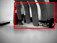
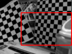
(a) Ground Truth

(b) RIFE

(c) EMA-VFI

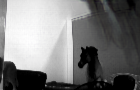
(d) Time Lens

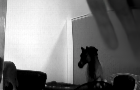
(e) Ours

Figure 6: Visual comparison among our proposed method, the state-of-the-art methods RIFE, EMA-VFI and Time Lens on HQF dataset containing real-world events.

4.3 Ablation Study

After step-by-step processing of each proposed module, the quality of output has been gradually improved. The results of each module are shown in Figure.1(b).

Effect of Gumbel Gating Module. In order to verify the effectiveness of our proposed method for reducing computational consumption, we input all sub-graphs as dynamic regions into the residual optical flow estimation network, and the test results are shown in the third and fourth row of Table.3. Compared with the method of considering all the sub-graphs as dynamic regions, the Tera-FLOPs and runtime of our proposed method tested on Vimeo90K-Triplet dataset greatly drops by 17% and 10.6% respectively, while the PSNR and SSIM merely decrease by 0.3dB and 0.001 individually.

Table 3: Quantitative comparison of the proposed method of Gumbel gating module for calculating residual optical flow, the method without residual optical flow estimation module and the method of calculating residual optical flow of all the sub-regions. These methods are tested on Vimeo90K-Triplet validation set. Runtime is the total time to run the entire dataset. Tera-FLOPs indicates a trillion floating-point operations.

Method	Runtime(s)$\downarrow$	Tera-FLOPs$\downarrow$	PSNR$\uparrow$	SSIM$\uparrow$
Without refinement	263	0.145	37.19	0.967
All regions process	442	0.253	39.40	0.977
Ours	395($\downarrow$10.6%)	0.210($\downarrow$17.0%)	39.10	0.976

Effect of Residual Optical Flow Estimation Module. We input the warping-based frames $I_{0}^{warp}$, $I_{1}^{warp}$ generated on the rough optical flow estimation and the boundary frames $I_{0}$, $I_{1}$ into the final synthesis module, for verifying the effect of our proposed residual optical flow module on improving the final result. The experimental results are shown in the second row of Table.3.

Effect of Cross-region Partition. We set the size of the sliding window to be H/2$\times$W/2, which is consistent with our proposed method. In addition, the step size is set to H/2$\times$W/2 in the vertical and horizontal directions respectively, which will produce four regions without any cross-region parts. They are fed into our proposed residual optical flow estimation network for training. The test results on Vimeo90K are shown in Table.4. Compared with the non-cross-region scheme, the proposed method with cross-region partition has a PSNR improvement of 1.68dB and a SSIM improvement of 0.008, which proves the effect of our method. As the cross-region part takes into account the correlation between domains, the optical flow estimation is smoother.

Table 4: Quantitative comparison of whether the region division includes cross-region partition on residual optical flow estimation module.

Region setting	PSNR$\uparrow$	SSIM$\uparrow$
Without Cross-region partition	31.33	0.948
Cross-region partition	33.01	0.956

5 Conclusion and Discussion

We have proposed an event-and-frame-based VFI method for dynamically estimating optical flow and residual optical flow between adjacent frames, which maintains high-quality output while reducing computation time and overhead by 10% and 17% respectively. Tests on several large-scale VFI benchmark datasets show that our proposed method outperforms other state-of-the-art VFI methods in terms of PSNR and SSIM. Limitations. On account of the lack of photometric information for events, IDO-VFI performs as deficiently as other VFI methods in scenes with complex photometric changes. In the future, we will consider introducing a contrast maximization method and a photometric loss function to reconstruct sharp edges and luminosity in those challenging scenes. Potential Negative Social Impacts. The proposed method can be used in application scenarios such as modal analysis and monitoring. These applications may bring concerns such as public privacy and security issue to the society. Please use the VFI technology reasonably under the premise of complying with the laws and regulations of various countries.

References

- (1) Christoph Posch, Teresa Serrano-Gotarredona, Bernabe Linares-Barranco, and Tobi Delbruck. Retinomorphic event-based vision sensors: bioinspired cameras with spiking output. Proc. IEEE, 102(10):1470–1484, 2014.
- (2) Deqing Sun, Xiaodong Yang, Ming-Yu Liu, and Jan Kautz. Pwc-net: Cnns for optical flow using pyramid, warping, and cost volume. In Proceedings of the IEEE conference on computer vision and pattern recognition, pages 8934–8943, 2018.
- (3) Huaizu Jiang, Deqing Sun, Varun Jampani, Ming-Hsuan Yang, Erik Learned-Miller, and Jan Kautz. Super slomo: High quality estimation of multiple intermediate frames for video interpolation. In Proceedings of the IEEE conference on computer vision and pattern recognition, pages 9000–9008, 2018.
- (4) Wenbo Bao, Wei-Sheng Lai, Chao Ma, Xiaoyun Zhang, Zhiyong Gao, and Ming-Hsuan Yang. Depth-aware video frame interpolation. In Proceedings of the IEEE/CVF Conference on Computer Vision and Pattern Recognition, pages 3703–3712, 2019.
- (5) Junheum Park, Keunsoo Ko, Chul Lee, and Chang-Su Kim. Bmbc: Bilateral motion estimation with bilateral cost volume for video interpolation. In European Conference on Computer Vision, pages 109–125. Springer, 2020.
- (6) Simon Niklaus and Feng Liu. Softmax splatting for video frame interpolation. In Proceedings of the IEEE/CVF Conference on Computer Vision and Pattern Recognition, pages 5437–5446, 2020.
- (7) Hyeonjun Sim, Jihyong Oh, and Munchurl Kim. Xvfi: Extreme video frame interpolation. In Proceedings of the IEEE/CVF International Conference on Computer Vision, pages 14489–14498, 2021.
- (8) Zhiyang Yu, Yu Zhang, Xujie Xiang, Dongqing Zou, Xijun Chen, and Jimmy S Ren. Deep bayesian video frame interpolation. In Computer Vision–ECCV 2022: 17th European Conference, Tel Aviv, Israel, October 23–27, 2022, Proceedings, Part XV, pages 144–160. Springer, 2022.
- (9) Xiangyu Xu, Li Siyao, Wenxiu Sun, Qian Yin, and Ming-Hsuan Yang. Quadratic video interpolation. Advances in Neural Information Processing Systems, 32, 2019.
- (10) Junheum Park, Chul Lee, and Chang-Su Kim. Asymmetric bilateral motion estimation for video frame interpolation. In Proceedings of the IEEE/CVF International Conference on Computer Vision, pages 14539–14548, 2021.
- (11) Hyeongmin Lee, Taeoh Kim, Tae-young Chung, Daehyun Pak, Yuseok Ban, and Sangyoun Lee. Adacof: Adaptive collaboration of flows for video frame interpolation. In Proceedings of the IEEE/CVF Conference on Computer Vision and Pattern Recognition, pages 5316–5325, 2020.
- (12) Myungsub Choi, Suyoung Lee, Heewon Kim, and Kyoung Mu Lee. Motion-aware dynamic architecture for efficient frame interpolation. In Proceedings of the IEEE/CVF International Conference on Computer Vision, pages 13839–13848, 2021.
- (13) Zhihao Shi, Xiangyu Xu, Xiaohong Liu, Jun Chen, and Ming-Hsuan Yang. Video frame interpolation transformer. In Proceedings of the IEEE/CVF Conference on Computer Vision and Pattern Recognition, pages 17482–17491, 2022.
- (14) Simon Niklaus, Ping Hu, and Jiawen Chen. Splatting-based synthesis for video frame interpolation. In Proceedings of the IEEE/CVF Winter Conference on Applications of Computer Vision, pages 713–723, 2023.
- (15) Wentao Shangguan, Yu Sun, Weijie Gan, and Ulugbek S Kamilov. Learning cross-video neural representations for high-quality frame interpolation. In Computer Vision–ECCV 2022: 17th European Conference, Tel Aviv, Israel, October 23–27, 2022, Proceedings, Part XV, pages 511–528. Springer, 2022.
- (16) Jihyong Oh and Munchurl Kim. Demfi: deep joint deblurring and multi-frame interpolation with flow-guided attentive correlation and recursive boosting. In Computer Vision–ECCV 2022: 17th European Conference, Tel Aviv, Israel, October 23–27, 2022, Proceedings, Part VII, pages 198–215. Springer, 2022.
- (17) Liyuan Pan, Cedric Scheerlinck, Xin Yu, Richard Hartley, Miaomiao Liu, and Yuchao Dai. Bringing a blurry frame alive at high frame-rate with an event camera. In Proceedings of the IEEE/CVF Conference on Computer Vision and Pattern Recognition, pages 6820–6829, 2019.
- (18) Zihao W Wang, Peiqi Duan, Oliver Cossairt, Aggelos Katsaggelos, Tiejun Huang, and Boxin Shi. Joint filtering of intensity images and neuromorphic events for high-resolution noise-robust imaging. In Proceedings of the IEEE/CVF Conference on Computer Vision and Pattern Recognition, pages 1609–1619, 2020.
- (19) Zhiyang Yu, Yu Zhang, Deyuan Liu, Dongqing Zou, Xijun Chen, Yebin Liu, and Jimmy S Ren. Training weakly supervised video frame interpolation with events. In Proceedings of the IEEE/CVF International Conference on Computer Vision, pages 14589–14598, 2021.
- (20) Stepan Tulyakov, Daniel Gehrig, Stamatios Georgoulis, Julius Erbach, Mathias Gehrig, Yuanyou Li, and Davide Scaramuzza. Time lens: Event-based video frame interpolation. In Proceedings of the IEEE/CVF Conference on Computer Vision and Pattern Recognition, pages 16155–16164, 2021.
- (21) Stepan Tulyakov, Alfredo Bochicchio, Daniel Gehrig, Stamatios Georgoulis, Yuanyou Li, and Davide Scaramuzza. Time lens++: Event-based frame interpolation with parametric non-linear flow and multi-scale fusion. In Proceedings of the IEEE/CVF Conference on Computer Vision and Pattern Recognition, pages 17755–17764, 2022.
- (22) Weihua He, Kaichao You, Zhendong Qiao, Xu Jia, Ziyang Zhang, Wenhui Wang, Huchuan Lu, Yaoyuan Wang, and Jianxing Liao. Timereplayer: Unlocking the potential of event cameras for video interpolation. In Proceedings of the IEEE/CVF Conference on Computer Vision and Pattern Recognition, pages 17804–17813, 2022.
- (23) Xiang Zhang and Lei Yu. Unifying motion deblurring and frame interpolation with events. In Proceedings of the IEEE/CVF Conference on Computer Vision and Pattern Recognition, pages 17765–17774, 2022.
- (24) Song Wu, Kaichao You, Weihua He, Chen Yang, Yang Tian, Yaoyuan Wang, Ziyang Zhang, and Jianxing Liao. Video interpolation by event-driven anisotropic adjustment of optical flow. In Computer Vision–ECCV 2022: 17th European Conference, Tel Aviv, Israel, October 23–27, 2022, Proceedings, Part VII, pages 267–283. Springer, 2022.
- (25) Alex Zihao Zhu, Liangzhe Yuan, Kenneth Chaney, and Kostas Daniilidis. Unsupervised event-based optical flow using motion compensation. In Proceedings of the European Conference on Computer Vision (ECCV) Workshops, pages 0–0, 2018.
- (26) Eric Jang, Shixiang Gu, and Ben Poole. Categorical reparametrization with gumble-softmax. In International Conference on Learning Representations (ICLR 2017). OpenReview. net, 2017.
- (27) Tianfan Xue, Baian Chen, Jiajun Wu, Donglai Wei, and William T Freeman. Video enhancement with task-oriented flow. International Journal of Computer Vision, 127(8):1106–1125, 2019.
- (28) Simon Baker, Daniel Scharstein, JP Lewis, Stefan Roth, Michael J Black, and Richard Szeliski. A database and evaluation methodology for optical flow. International Journal of Computer Vision, 92(1):1–31, 2011.
- (29) Seungjun Nah, Tae Hyun Kim, and Kyoung Mu Lee. Deep multi-scale convolutional neural network for dynamic scene deblurring. In Proceedings of the IEEE/CVF Conference on Computer Vision and Pattern Recognition, pages 3883–3891, 2017.
- (30) Henri Rebecq, René Ranftl, Vladlen Koltun, and Davide Scaramuzza. Events-to-video: Bringing modern computer vision to event cameras. In Proceedings of the IEEE/CVF Conference on Computer Vision and Pattern Recognition, pages 3857–3866, 2019.
- (31) Haopeng Li, Yuan Yuan, and Qi Wang. Video frame interpolation via residue refinement. In Proceedings of the International Conference on Acoustics, Speech and Signal Processing, pages 2613–2617. IEEE, 2020.
- (32) Zhewei Huang, Tianyuan Zhang, Wen Heng, Boxin Shi, and Shuchang Zhou. Real-time intermediate flow estimation for video frame interpolation. In Computer Vision–ECCV 2022: 17th European Conference, Tel Aviv, Israel, October 23–27, 2022, Proceedings, Part XIV, pages 624–642. Springer, 2022.
- (33) Guozhen Zhang, Yuhan Zhu, Haonan Wang, Youxin Chen, Gangshan Wu, and Limin Wang. Extracting motion and appearance via inter-frame attention for efficient video frame interpolation. In Proceedings of the IEEE/CVF Conference on Computer Vision and Pattern Recognition, 2023.
- (34) Junheum Park, Jintae Kim, and Chang-Su Kim. Biformer: Learning bilateral motion estimation via bilateral transformer for 4k video frame interpolation. In Proceedings of the IEEE/CVF Conference on Computer Vision and Pattern Recognition, 2023.
- (35) Henri Rebecq, Daniel Gehrig, and Davide Scaramuzza. Esim: an open event camera simulator. In Conference on robot learning, pages 969–982. PMLR, 2018.
- (36) Diederik P Kingma and Jimmy Ba. Adam: A method for stochastic optimization. arXiv preprint arXiv:1412.6980, 2014.
- (37) Timo Stoffregen, Cedric Scheerlinck, Davide Scaramuzza, Tom Drummond, Nick Barnes, Lindsay Kleeman, and Robert Mahony. Reducing the sim-to-real gap for event cameras. In Proceedings of the European Conference on Computer Vision, pages 534–549. Springer, 2020.
- (38) Zhou Wang, Alan C Bovik, Hamid R Sheikh, and Eero P Simoncelli. Image quality assessment: from error visibility to structural similarity. IEEE Transactions on Image Processing, 13(4):600–612, 2004.