Dynamic Structural Brain Network Construction by Hierarchical Prototype Embedding GCN using T1-MRI

Abstract

Constructing structural brain networks using T1-weighted magnetic resonance imaging (T1-MRI) presents a significant challenge due to the lack of direct regional connectivity information. Current methods with T1-MRI rely on predefined regions or isolated pretrained location modules to obtain atrophic regions, which neglects individual specificity. Besides, existing methods capture global structural context only on the whole-image-level, which weaken correlation between regions and the hierarchical distribution nature of brain connectivity. We hereby propose a novel dynamic structural brain network construction method based on T1-MRI, which can dynamically localize critical regions and constrain the hierarchical distribution among them for constructing dynamic structural brain network. Specifically, we first cluster spatially-correlated channel and generate several critical brain regions as prototypes. Further, we introduce a contrastive loss function to constrain the prototypes distribution, which embed the hierarchical brain semantic structure into the latent space. Self-attention and GCN are then used to dynamically construct hierarchical correlations of critical regions for brain network and explore the correlation, respectively. Our method is evaluated on ADNI-1 and ADNI-2 databases for mild cognitive impairment (MCI) conversion prediction, and acheive the state-of-the-art (SOTA) performance. Our source code is available at http://github.com/*******.

1 Introduction

T1-weighted magnetic resonance imaging (T1-MRI) is one of the indispensable medical imaging methods for noninvasive diagnosing neurological disorder [9]. Existing approaches [16, 19] based on T1-MRI focus on extracting region of interests (ROIs) to analyze structural atrophy information associated with disease progression. However, some works [16, 21, 6] heavily rely on manual defined and selected ROIs, which have limitations in explaining the individual brain specificity. To address this issue, Lian et al. [15] localize discriminative regions by a pretrained module, where region localization and following feature learning cannot reinforce each other, resulting a coarse feature representation. Additionally, as inter-regional correlations are unavailable in T1-MRI directly, most related works [2, 14] ignore inter-regional correlations or replace them with a generalized global information. These conventional modular approaches have limitations in explaining high-dimensional brain structure information [1, 25].

Brain network is a vital method to analysis brain disease, which has been widely used in functional magnetic resonance imaging (fMRI) and diffusion tensor imaging (DTI). However, the structural brain network with T1-MRI is still underexplored due to the lack of direct regional connectivity. Recent advances [11, 22, 23, 8] in graph convolution neural networks (GCNs) have optimized brain networks construction with fMRI and DTI. Given the successful application of GCN in these modalities, we think that it also has potential for construction of structural brain network using T1-MRI. Current approaches [4, 12, 13, 8] to brain network construction involve the selection of ROIs and modeling inter-regional correlations, in which anatomical ROIs are employed as nodes, and inter-node correlations are modeled as edges. Some researches[30, 18] have demonstrated that brain connectivity displays hierarchical structure distribution, yet most GCN-based methods[27, 13] treat all nodes equally and ignore the hierarchical nature of brain connectivity. These structural brain networks are fixed and redundant, which may lead to coarse feature representation and suboptimal performance in downstream tasks.

To address these issues, we propose novel dynamic structural brain network construction method named hierarchical prototypes embedding GCN (DH-ProGCN) to dynamically construct disease-related structural brain network based on T1-MRI. Firstly, a prototypes learning method is used to cluster spatially-correlated channel and generate several critical brain regions as prototypes. Then, we introduce a contrastive loss function to constrain the hierarchical distribution among prototypes to obtain the hierarchical brain semantic structure embdedding in the latent space. After that, DH-ProGCN utilizes a self-attention mechanism to dynamically construct hierarchical correlations of critical regions for constructing structural brain network. GCN is applied to explore the correlation of the structural brain network for Mild Cognitive Impairment (MCI) conversion prediction. We verify the effectiveness of DH-ProGCN on the Alzheimer’s Disease Neuroimaging Initiative-1 (ADNI-1) and ADNI-2 dataset. DH-ProGCN achieves state-of-the-art (SOTA) performance for the the classification of progressive mild cognitive impairment (pMCI) and stable mild cognitive impairment (sMCI) based on T1-MRI.

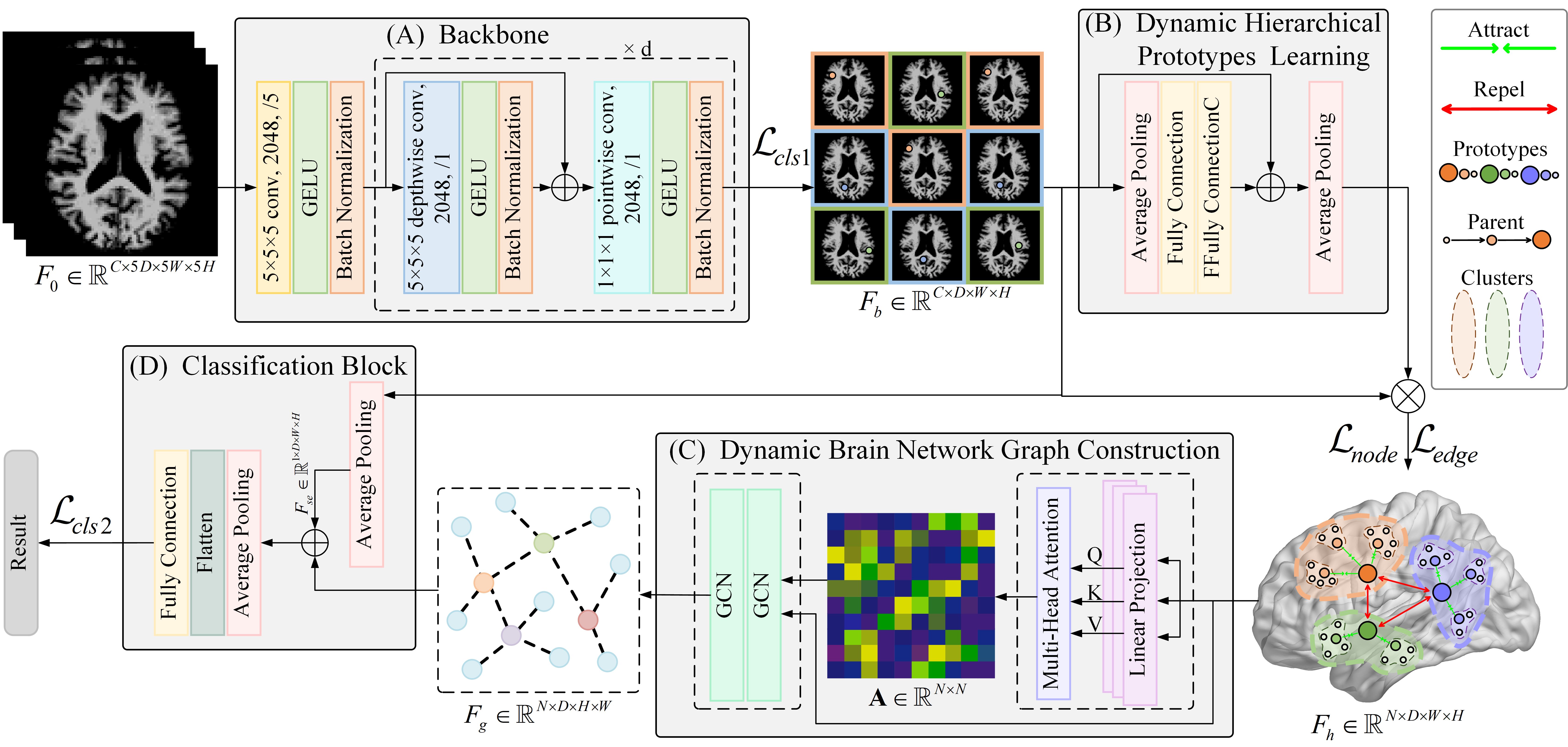
Figure 1: The overall framework of the DH-ProGCN. (A) We first extract the feature $F_{b}$ via backbone, and assume that the featuremap of each channel represents different discriminative regions which are showed as images with different colors in $F_{b}$. (B) The hierarchical feature $F_{h}$ are then obtained by hierarchical clustering on the channel dimension. (C) We utilize a self-attention mechanism to model feature correlations matrix $A$ and learn the feature graph $F_{g}$ by a GCN. (D) $F_{g}$ and the global representation $F_{b}$ are concatenated for MCI conversion prediction.

2 Methods

2.1 Backbone

In this study, we utilize a Convmixer-like [24] block as the backbone to achieve primary discriminative brain regions localization, which could provide a large enough channel dimension for subsequent channel clustering with relatively low complexity. Specifically, depicted in Fig. 1(A), the backbone consists of a patch embedding layer followed by several full-convolution blocks. Patch embedding comprises a $5\times 5\times 5$ convolution, and the full convolution block comprikuaijses a $5\times 5\times 5$ depthwise convolution (grouped convolution with groups equal to the number of channels) and a pointwise convolution (kernel size is $1\times 1\times 1$) with 2048 channels. By the backbone, features of discriminative regions are finally extracted as $F_{b}\in{\mathbb{R}}^{C\times D\times H\times W}$, where $D$, $H$, $W$ and $C$ indicate depth, height, width and the number of channels, respectively.

2.2 Dynamic Hierarchical Prototype Learning

2.2.1 Prototypes Definition.

In this study, we regard feature maps of each channel as corresponding to the response of distinct brain regions relevant to tasks. Following [29], we utilize the location of each peak response as the channel information. Intuitively, a position vector composed of peak response coordinates of each channel is defined as the candidate prototype. Position vectors of training images can be obtained as following:

$$[t_{x}^{1},t_{y}^{1},t_{z}^{1},t_{x}^{2},t_{y}^{2},t_{z}^{2},\ldots,t_{x}^{\Omega},t_{y}^{\Omega},t_{z}^{\Omega}]$$ (1)

where $[t_{x}^{i}$, $t_{y}^{i}$, $t_{z}^{i}]$ represents the peak response coordinate of the $i$-$th$ image and $\Omega$ represents the number of images in the training set. $K$-means [17] is used to achieve prototypes initialization. Specifically, vectors of all channels are clustered to obtain $N$ sets of clusters $K={\{k_{n}\}}_{n=1}^{N}$, and prototypes are defined as clustering centers $\Gamma=\{\gamma_{n}\}_{n=1}^{N}$ which are taken as $N$ critical regions for the discriminative localization (i.e., ROIs). $F_{h}\in\mathbb{R}^{N\times D\times H\times W}$ represents features of clustering centers.

2.2.2 Dynamic Hierarchical Prototype Exploring.

Inter-regional spatial connectivity is fixed, but the correlation between them is dynamic with disease progression. We argue that there are structural correlations between different regions, just as the complex hierarchical functional connectome in rich-clubs [25] organization with fMRI. We therefore explore the hierarchical semantic structure of critical brain regions by the hierarchical prototype clustering method.

Specifically, we start by using the initial prototypes as the first hierarchy clustering prototypes, denoted as $\Gamma^{0}=\{\gamma_{n}^{0}\}_{n=1}^{N_{0}}$. Then, $K$-means is applied iteratively to obtain parent prototypes of the lower-hierarchy prototypes $\Gamma^{i-1}=\{\gamma_{n}^{i-1}\}_{n=1}^{N_{i-1}}$, denoted as $\Gamma^{i}=\{\gamma_{n}^{i}\}_{n=1}^{N_{i}}$, where $i$ represents the $i$-$th$ hierarchy and $N_{i}$ represents the number of clusters at $i$-$th$ hierarchy, corresponding to the cluster $K^{i}={\{k_{n}^{i}\}}_{n=1}^{N_{i}}$. In this paper, $i$ is set as 2. The number of prototypes in the first, second and third hierarchy is set as 16, 8 and 4, respectively.

To facilitate optimal clustering of the network during training, we use two fully convolutional layers with two contrastive learning loss functions $\mathcal{L}_{node}$ and $\mathcal{L}_{edge}$ to approximate the clustering process. With $\mathcal{L}_{node}$, each channel clustering is enforced to become more compact inside and have significant inter-class differences with other clusterings, enabling all prototypes to be well separated:

$$\mathcal{L}_{node}=\displaystyle-\frac{1}{L}\sum_{l=1}^{L}\sum_{n=1}^{N_{l}}\displaystyle\sum_{u\in K_{n}^{l}}\log\frac{\exp\left(u\cdot\gamma_{n}^{l}/\phi_{n}^{l}\right)}{\sum_{i\neq n}^{N_{l}}\exp\left(u\cdot\gamma_{i}^{l}/\phi_{n}^{l}\right)}$$ (2)

$$\phi_{n}^{l}=\frac{\sum_{u\in K_{n}^{l}}\left\|u-\gamma_{n}^{l}\right\|_{2}}{|K_{n}^{l}|\cdot\log(|K_{n}^{l}|+\alpha)}$$ (3)

Where $L$ is the total number of layers, and $N_{l}$ is the number of clusters in the $l$-$th$ layer. $K_{n}^{l}$, $\gamma_{n}^{l}$, and $\phi_{n}^{l}$ denote the set of all elements, the cluster center (prototype), and the estimation of concentration of the $n$-$th$ cluster in the $l$-$th$ layer, respectively. $\alpha$ is a smoothing parameter to prevent small clusters from having overly-large $\phi$.

The cluster concentration $\phi$ measures the closeness of elements in a cluster. A larger $\phi$ indicates more elements in the cluster or smaller total average distance between all elements and the cluster center. Ultimately, $\mathcal{L}_{node}$ compels all elements $u$ in $K_{n}^{l}$ to be close to their cluster center $\gamma_{n}^{l}$ and away from other cluster center at the same level.

Similarly, $\mathcal{L}_{edge}$ aims to embed the hierarchical correlation between clustering prototypes, which can be expressed as:

$$\mathcal{L}_{edge}=\displaystyle-\frac{1}{L}\sum_{l=1}^{L-1}\displaystyle\sum_{n=1}^{N_{l}}\log\frac{\exp\left(\gamma_{n}^{l}\cdot Parent(\gamma_{n}^{l})/\tau\right)}{\sum_{i\neq n}^{N^{l}}\exp\left(\gamma_{n}^{l}\cdot\gamma_{i}^{l}/\tau\right)}$$ (4)

$Parent(\gamma_{n}^{l})$ represents the parent prototype of the prototype $\gamma_{n}^{l}$, and $\tau$ is a temperature hyper-parameter. $\mathcal{L}_{edge}$ forces all prototypes $\gamma^{l}$ in the $l$-$th$ layer to be close to their parent prototype and away from other prototypes within the same level.

2.3 Brain Network Graph Construction and Classification

Through Section 2.2, critical brain regions are clustered in a hierarchical semantic latent space. We hereby employ the prototypes regions as nodes and correlations between them as edges to construct structural brain network graphs as shown in Fig. 1(C).

We first apply a self-attention mechanism [26] to compute inter-region correlations to generate edges of the brain network. Then, the features $F_{h}$ is input to three separate fully connected layers to obtain three vectors: query, key, and value, which are used to compute attention scores $\mathbf{A}\in\mathbb{R}^{N\times N}$ between each pair of prototypes, followed by being used to weight the value vector and obtain the output of the self-attention layer as following operation:

$$\mathbf{A}=Attention(Q,K,V)=softmax(\frac{QK^{T}}{\sqrt[]{d_{k}}})V$$ (5)

where $Q\in\mathbb{R}^{N\times d_{k}}$, $K\in\mathbb{R}^{N\times d_{k}}$, $V\in\mathbb{R}^{N\times N}$ denote query, key, and value, respectively. $d_{k}$ represents the dimension of $Q$, $K$. $N$ represents the number of critical regions, which is set as 16 in this paper.

We then employ GCN to capture the topological interaction in the brain network graph and update features of nodes by performing the following operation:

$$GCN(\mathbf{X})=\operatorname{ReLU}\left(\hat{\mathbf{D}}^{-1/2}\hat{\mathbf{A}}\hat{\mathbf{D}}^{-1/2}\mathbf{X}\Theta\right)$$ (6)

where $\hat{\mathbf{A}}=\mathbf{A}+\mathbf{I}$ is the adjacency matrix with inserted self-loops and $\mathbf{I}$ denotes an identity matrix. $\hat{\mathbf{D}}_{ii}=\sum_{j=0}\hat{\mathbf{A}}_{ij}$ is the diagonal degree matrix, and $\Theta$ represents learned weights. To prevent the network overfitting, we just use two GCN layers as the encoder to obtain the final graph feature $F_{g}\in\mathbb{R}^{N\times D\times H\times W}$.

To this end, the information of critical brain regions are fully learned. Notably, as prototypes are dynamic, constructed brain network graphs are also dynamic, rather than predefined and fixed. This allows DH-ProGCN to model and explore the individual hierarchical information, providing a more personalise brain network representation for every subject.

To achieve the classification, we perform channel squeezing on the backbone feature $F_{b}$ to obtain global features $F_{se}\in\mathbb{R}^{1\times D\times H\times W}$, concatenate it with $F_{g}$ and input them into the classification layer.

3 Experiments

3.1 Dataset

The data we used are from two public databases: ADNI-1 (http://www.adni-info.org) [20], and ADNI-2. The demographic information of the subjects and preprocessing steps are shown in the supplemental material. The preprocessed images are finally resized to $91\times 109\times 91$ voxels. Through the quality checking, 305 images are left from ADNI-1 (197 for sMCI, 108 for pMCI), and 250 images are left from ADNI-2 (251 for sMCI, 99 for pMCI). Note that some subjects have two images or more in different times, and we only keep the earliest one. Following [15], we train DH-ProGCN on ADNI-1 and perform independent testing on ADNI-2.

3.2 Implementation Details

We first train backbone with 2048 channels in all layers to extract the output features $F_{b}$ with the cross-entropy loss $\mathcal{L}_{cls1}$. The cross-entropy loss $\mathcal{L}_{cls2}$ is used for the final classification. The overall loss function is defined as:

$$\mathcal{L}=\mathcal{L}_{cls1}+\mathcal{L}_{cls2}+\mathcal{L}_{node}+\mathcal{L}_{edge}$$ (7)

where $\mathcal{L}_{node}$ and $\mathcal{L}_{edge}$ are explained in Section 2.2. Smooth parameter $\alpha=10$ and temperature parameter $\tau=0.2$ following [3].

All blocks are trained by SGD optimizer with a momentum of 0.9 and weight decay of 0.001. The model is trained for 300 epochs with an initial learning rate of 0.01 that is decreased by a factor of 10 every 100 epochs. Five metrics, namely accuracy (ACC), sensitivity (SEN), specificity (SPE), and area under the curve (AUC), are used to evaluate the performance of the proposed model. We use Python based on the PyTorch package and run the network on a single NVIDIA GeForce 3090 24 GB GPU.

4 Results

4.1 Comparing with SOTA Methods

Six SOTA methods are used for comparison: 1) LDMIL [16] captured both local information conveyed by patches and global information; 2) H-FCN [15] implemented three levels of networks to obtain multi-scale feature representations which are fused for the construction of hierarchical classifiers; 3) HybNet [14] assigned the subject-level label to patches for local feature learning by iterative network pruning; 4) AD²A [10] located discriminative disease-related regions by an attention modules; 5) DSNet [19] provided disease-image specificity to an image synthesis network; 6) MSA3D [2] implemented a slice-level attention and a 3D CNN to capture subject-level structural changes.

Results in Table 1 show the superiority of DH-ProGCN over SOTA approaches for MCI conversion prediction. Specifically, DH-ProGCN achieves ACC of 0.849 and AUC of 0.845 tested on ADNI-2 by models trained on ADNI-1. It is worth noting that our method: 1) needs no predefined manual landmarks, but achieves better diagnostic results than existing deep-learning-based MCI diagnosis methods; 2) needs no pretrain network parameters from other tasks like AD diagnosis; 3) introduces hierarchical distribution structure to connect regions and form region-based specificity brain structure networks, rather than generalizing the correlations between regions with global information.

Table 1: Comparsion of our method with current SOTA methods for MCI conversion prediction on ADNI-2 obtained by the models trained on ADNI-1.

Method	ACC	SEN	SPE	AUC
LDMIL	0.769	0.421	0.824	0.776
H-FCN	0.809	0.526	0.854	0.781
HybNet	0.827	0.579	0.866	0.793
AD2A	0.780	0.534	0.866	0.788
DSNet	0.762	0.770	0.742	0.818
MSA3D	0.801	0.520	0.856	0.789
DH-ProGCN	0.849	0.647	0.928	0.845

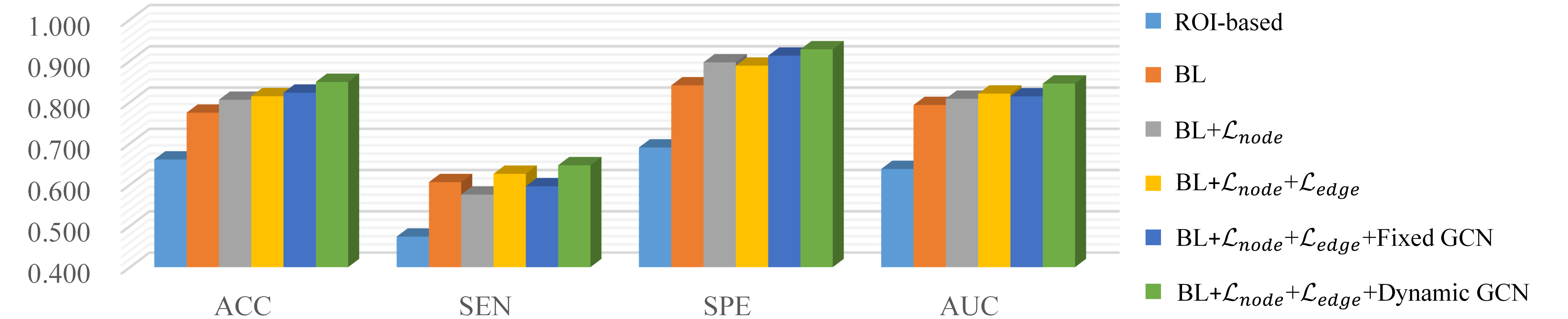
Figure 2: Effects of each component of DH-ProGCN for MCI conversion prediction on ADNI-2 obtained by models trained on ADNI-1.

4.2 Ablation Study

4.2.1 Effect of dynamic prototype learning.

To verify the effect of dynamic prototype clustering, we compare 1) ROI-based approach [28], 2) backbone without channel clustering (BL), 3) backbone with dynamic prototypes clustering (BL+$\mathcal{L}_{node}$). As shown in Fig. 2, results indicate that dynamic prototype clustering outperforms the ROI-based and backbone on MCI conversion, and could generate better feature distributions for downstream brain images analysis tasks.

4.2.2 Effect of Hierarchical prototype learning.

To evaluate the impact of hierarchical prototype learning, we compare backbone with flattened prototypes clustering (BL+$\mathcal{L}_{node}$), and hierarchical clustering (BL+$\mathcal{L}_{node}$+$\mathcal{L}_{edge}$). The results are presented in Fig. 2. With the constraint strengthened on the distribution of regions, the results are progressively improved. This implies that it makes sense to introduce hierarchical semantics into the construction of structure brain networks.

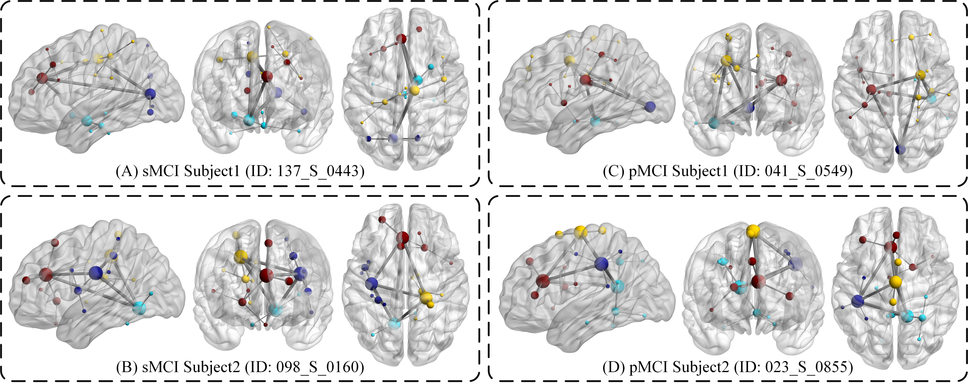
Figure 3: Sagittal, coronal and axial views of connectome in hierarchical critical regions. (A)(B) represent brain network visualization of sMCI and (C)(D) represent pMCI subjects. Nodes correspond to critical regions i.e. prototypes, and edges are form the connectivity weight between nodes. The size of node increases with its hierarchy, and nodes with same color are clustered into the same parent prototype. Lower-hierarchy prototypes within cluster are closer to its parent prototypes, and higher-hierarchy prototypes between different clusters are closer than lower-hierarchy prototypes.

4.2.3 Effect of Dynamic Brain Network Construction.

To verify whether our constructed dynamic brain network capability outperforms the fixed architecture, we obtained the fixed brain network graph by directly connecting all critical regions after obtaining hierarchical features and feeding them into the GCN for classification. The results are shown in Fig. 2, where the dynamic brain network structure performs better, suggesting that the correlation between regions needs to be measured dynamically to construct a better brain network.

In addition, we visualize the sagittal, coronal and axial views of hierarchical critical regions and their connectome in Fig. 3. The left and right sub-figures represent brain network visualization of two sMCI and two pMCI subjects, respectively. In general, critical regions and correlations are varied for different subjects, which means that our method is feasible for constructing individual brain networks according to the individuals specificity. Localized regions are roughly distributed in anatomically defined parahippocampal gyrus, superior frontal gyrus, and cingulate gyrus for different sMCI subjects, lingual gyrus right, and superior longitudinal fasciculus for different pMCI subjects, which agree with previous studies. [9, 5, 7].

5 Conclusion

In this paper, we propose a novel dynamic structural brain network construction method named DH-ProGCN. DH-ProGCN could dynamically cluster critical brain regions by the prototype learning, implicitly encode the hierarchical semantic structure of the brain into the latent space by hierarchical prototypes embedding, dynamically construct brain networks by self-attention and extract topology features in the brain network by GCN. Experimental results show that DH-ProGCN outperforms SOTA methods on the MCI conversion task. Essentially, DH-ProGCN has the potential to model hierarchical topological structures in other kinds of medical images. In our future work, we will apply this framework to other kinds of modalities and neurological disorders.

5.0.1 Acknowledgements

This work is partially supported by ********* and ********.

References

- [1] Ed Bullmore and Olaf Sporns. Complex brain networks: graph theoretical analysis of structural and functional systems. Nature reviews neuroscience, 10(3):186–198, 2009.
- [2] Lin Chen, Hezhe Qiao, and Fan Zhu. Alzheimer’s disease diagnosis with brain structural mri using multiview-slice attention and 3d convolution neural network. Frontiers in Aging Neuroscience, 14, 2022.
- [3] Xinlei Chen, Haoqi Fan, Ross Girshick, and Kaiming He. Improved baselines with momentum contrastive learning. arXiv preprint arXiv:2003.04297, 2020.
- [4] Yuzhong Chen, Jiadong Yan, Mingxin Jiang, Tuo Zhang, Zhongbo Zhao, Weihua Zhao, Jian Zheng, Dezhong Yao, Rong Zhang, Keith M Kendrick, et al. Adversarial learning based node-edge graph attention networks for autism spectrum disorder identification. IEEE Transactions on Neural Networks and Learning Systems, 2022.
- [5] Andrea Chincarini, Paolo Bosco, Piero Calvini, Gianluca Gemme, Mario Esposito, Chiara Olivieri, Luca Rei, Sandro Squarcia, Guido Rodriguez, Roberto Bellotti, et al. Local mri analysis approach in the diagnosis of early and prodromal alzheimer’s disease. Neuroimage, 58(2):469–480, 2011.
- [6] Wenju Cui, Caiying Yan, Zhuangzhi Yan, Yunsong Peng, Yilin Leng, Chenlu Liu, Shuangqing Chen, Xi Jiang, Jian Zheng, and Xiaodong Yang. Bmnet: A new region-based metric learning method for early alzheimer’s disease identification with fdg-pet images. Frontiers in Neuroscience, 16:831533, 2022.
- [7] Bradford C Dickerson, I Goncharova, MP Sullivan, C Forchetti, RS Wilson, DA Bennett, Laurel A Beckett, and L deToledo Morrell. Mri-derived entorhinal and hippocampal atrophy in incipient and very mild alzheimer’s disease. Neurobiology of aging, 22(5):747–754, 2001.
- [8] Fatih Said Duran, Abdurrahman Beyaz, and Islem Rekik. Dual-hinet: Dual hierarchical integration network of multigraphs for connectional brain template learning. In Medical Image Computing and Computer Assisted Intervention–MICCAI 2022: 25th International Conference, Singapore, September 18–22, 2022, Proceedings, Part I, pages 305–314. Springer, 2022.
- [9] Giovanni B Frisoni, Nick C Fox, Clifford R Jack Jr, Philip Scheltens, and Paul M Thompson. The clinical use of structural mri in alzheimer disease. Nature Reviews Neurology, 6(2):67–77, 2010.
- [10] Hao Guan, Yunbi Liu, Erkun Yang, Pew-Thian Yap, Dinggang Shen, and Mingxia Liu. Multi-site mri harmonization via attention-guided deep domain adaptation for brain disorder identification. Medical image analysis, 71:102076, 2021.
- [11] Thomas N Kipf and Max Welling. Semi-supervised classification with graph convolutional networks. arXiv preprint arXiv:1609.02907, 2016.
- [12] Baiying Lei, Nina Cheng, Alejandro F Frangi, Ee-Leng Tan, Jiuwen Cao, Peng Yang, Ahmed Elazab, Jie Du, Yanwu Xu, and Tianfu Wang. Self-calibrated brain network estimation and joint non-convex multi-task learning for identification of early alzheimer’s disease. Medical image analysis, 61:101652, 2020.
- [13] Yueting Li, Qingyue Wei, Ehsan Adeli, Kilian M Pohl, and Qingyu Zhao. Joint graph convolution for analyzing brain structural and functional connectome. In Medical Image Computing and Computer Assisted Intervention–MICCAI 2022: 25th International Conference, Singapore, September 18–22, 2022, Proceedings, Part I, pages 231–240. Springer, 2022.
- [14] Chunfeng Lian, Mingxia Liu, Yongsheng Pan, and Dinggang Shen. Attention-guided hybrid network for dementia diagnosis with structural mr images. IEEE transactions on cybernetics, 52(4):1992–2003, 2020.
- [15] Chunfeng Lian, Mingxia Liu, Jun Zhang, and Dinggang Shen. Hierarchical fully convolutional network for joint atrophy localization and alzheimer’s disease diagnosis using structural mri. IEEE transactions on pattern analysis and machine intelligence, 42(4):880–893, 2018.
- [16] Mingxia Liu, Jun Zhang, Ehsan Adeli, and Dinggang Shen. Landmark-based deep multi-instance learning for brain disease diagnosis. Medical image analysis, 43:157–168, 2018.
- [17] Stuart Lloyd. Least squares quantization in pcm. IEEE transactions on information theory, 28(2):129–137, 1982.
- [18] David Meunier, Renaud Lambiotte, Alex Fornito, Karen Ersche, and Edward T Bullmore. Hierarchical modularity in human brain functional networks. Frontiers in neuroinformatics, page 37, 2009.
- [19] Yongsheng Pan, Mingxia Liu, Yong Xia, and Dinggang Shen. Disease-image-specific learning for diagnosis-oriented neuroimage synthesis with incomplete multi-modality data. IEEE transactions on pattern analysis and machine intelligence, 44(10):6839–6853, 2021.
- [20] Ronald Carl Petersen, Paul S Aisen, Laurel A Beckett, Michael C Donohue, Anthony Collins Gamst, Danielle J Harvey, Clifford R Jack, William J Jagust, Leslie M Shaw, Arthur W Toga, et al. Alzheimer’s disease neuroimaging initiative (adni): clinical characterization. Neurology, 74(3):201–209, 2010.
- [21] Wei Shao, Yao Peng, Chen Zu, Mingliang Wang, Daoqiang Zhang, Alzheimer’s Disease Neuroimaging Initiative, et al. Hypergraph based multi-task feature selection for multimodal classification of alzheimer’s disease. Computerized Medical Imaging and Graphics, 80:101663, 2020.
- [22] Xuegang Song, Feng Zhou, Alejandro F Frangi, Jiuwen Cao, Xiaohua Xiao, Yi Lei, Tianfu Wang, and Baiying Lei. Graph convolution network with similarity awareness and adaptive calibration for disease-induced deterioration prediction. Medical Image Analysis, 69:101947, 2021.
- [23] Xuegang Song, Feng Zhou, Alejandro F Frangi, Jiuwen Cao, Xiaohua Xiao, Yi Lei, Tianfu Wang, and Baiying Lei. Multi-center and multi-channel pooling gcn for early ad diagnosis based on dual-modality fused brain network. IEEE Transactions on Medical Imaging, 2022.
- [24] Asher Trockman and J Zico Kolter. Patches are all you need? arXiv preprint arXiv:2201.09792, 2022.
- [25] Martijn P Van Den Heuvel and Olaf Sporns. Rich-club organization of the human connectome. Journal of Neuroscience, 31(44):15775–15786, 2011.
- [26] Ashish Vaswani, Noam Shazeer, Niki Parmar, Jakob Uszkoreit, Llion Jones, Aidan N Gomez, Łukasz Kaiser, and Illia Polosukhin. Attention is all you need. Advances in neural information processing systems, 30, 2017.
- [27] Jin Ye, Junjun He, Xiaojiang Peng, Wenhao Wu, and Yu Qiao. Attention-driven dynamic graph convolutional network for multi-label image recognition. In Computer Vision–ECCV 2020: 16th European Conference, Glasgow, UK, August 23–28, 2020, Proceedings, Part XXI 16, pages 649–665. Springer, 2020.
- [28] Daoqiang Zhang, Yaping Wang, Luping Zhou, Hong Yuan, Dinggang Shen, Alzheimer’s Disease Neuroimaging Initiative, et al. Multimodal classification of alzheimer’s disease and mild cognitive impairment. Neuroimage, 55(3):856–867, 2011.
- [29] Heliang Zheng, Jianlong Fu, Tao Mei, and Jiebo Luo. Learning multi-attention convolutional neural network for fine-grained image recognition. In Proceedings of the IEEE international conference on computer vision, pages 5209–5217, 2017.
- [30] Changsong Zhou, Lucia Zemanová, Gorka Zamora, Claus C Hilgetag, and Jürgen Kurths. Hierarchical organization unveiled by functional connectivity in complex brain networks. Physical review letters, 97(23):238103, 2006.