Self-interaction and transport of solvated electrons in molten salts

Abstract

The dynamics of (few) electrons dissolved in an ionic fluid—as when a small amount of metal is added to a solution while upholding its electronic insulation—manifests interesting properties that can be ascribed to nontrivial topological features of particle transport (e.g., Thouless’ pumps). In the adiabatic regime, the charge distribution and the dynamics of these dissolved electrons are uniquely determined by the nuclear configuration. Yet, their localization into effective potential wells and their diffusivity are dictated by how the self-interaction is modeled. In this article, we investigate the role of self-interaction in the description of localization and transport properties of dissolved electrons in non-stoichiometric molten salts. Although the account for the exact (Fock) exchange strongly localizes the dissolved electrons, decreasing their tunneling probability and diffusivity, we show that the dynamics of the ions and of the dissolved electrons are largely uncorrelated, irrespective of the degree to which the electron self-interaction is treated, and in accordance with topological arguments.

I Introduction

Extremely diluted alkali-metal/alkali-halide solutions feature solvated electrons released by the excess metal atoms that tend to localize in bound states analogous to polarons in dielectric solids.[1, 2, 3, 4, 5, 6, 7, 8, 9] Solvated electrons are the simplest anions in nature. They often appear as reaction intermediates in diverse chemical processes such as, e.g., radiolysis, photolysis, and electrolysis of polar materials.[10] Despite having been observed for more than two centuries, since solutions of potassium in gaseous ammonia were examined by Sir Humphry Davy,[11] their properties are far from being completely explained, with some important advancements in their full understanding having appeared relatively recently in the literature, aided by the increasing accuracy and affordability of electronic-structure and machine-learning methods.[12, 13, 14, 15]

Solvated electrons in molten metal-metal halide solutions have been experimentally investigated especially since the 1940s, when molten salts were employed in the context of nuclear technologies.[1, 16, 17, 18, 19, 20] Far from the NonMetal-to-Metal (NM-M) transition, the dynamics of such electronic states is adiabatic;[21, 22] therefore, the distribution of the excess electrons at each moment is entirely determined by the instantaneous ionic configuration, and the electronic motion is due to the ionic one.

The adiabatic variation of the potential energy surface determined by the nuclear dynamics is a natural playground for Thouless’ theory of charge pumping;[23, 24] in particular, the theorem of charge quantization, together with a recently discovered gauge invariance of transport coefficients,[25, 26, 27] provide a theoretical foundation for describing the charge-transport properties of ionic conductors according to the topology of their electronic structure. Notably, topological arguments demonstrate that in non-stoichiometric systems, which feature dissolved electrons, nontrivial charge transport can occur, meaning that adiabatic transport of charge can take place even without a net ionic displacement.[22, 28] This happens in non-stoichiometric molten salts such as metal/metal-halide solutions, where the electrical (ionic) conductivity can be recast as the sum of a part due to ions and one due to solvated electrons alone, the two contributions being uncorrelated from one another,[22, 28] resulting in a much increased electrical conductivity even before the NM-M transition.[2] The whole machinery behind these concepts is rooted in the modern theory of polarization;[29, 30] the latter provides also a means to rigorously characterize the electronically insulating state by exploiting its defining feature, i.e. the absence of dc conductivity, in terms of the localization of the electronic wavefunction.[31]

In practical calculations, electronic localization—and, vice versa, electronic diffusion—is determined by how self-interaction is accounted for in the employed theoretical framework. It is well known that standard Density Functional Theory (DFT) is affected by self-interaction errors due to the interaction of each electron with the total one-body electron density, including its own density.[32] The spurious contribution is partially removed by the approximate eXchange and Correlation (XC) functional, but errors are still large, especially for local and semi-local XC functionals.[32, 33] The excess electrons in metal-metal halide solutions are effectively few-electron systems and, as such, are particularly affected by spurious self-interactions.[33] Since fluids are structurally disordered materials, the localization of a small number of electrons is often facilitated with respect to crystalline systems, so even calculations employing semi-local XC functional result in rather localized electronic states whose dynamics has been studied from Ab Initio Molecular Dynamics (AIMD) simulations based on standard DFT.[3, 4, 5, 6, 21, 22] Nonetheless, the inclusion of a fraction of EXact (Fock) eXchange (EXX) naturally leads to a stronger degree of electronic localization, since EXX partially removes the effect of self-interaction, and helps describing, e.g., polarons in solids[34] and the localization in cavities of excess electrons in fluids.[14]

It is thus expected that the EXX would quantitatively alter the charge transport properties of an ionic system containing solvated electrons, as the latter tend to be more localized and their interaction with the ionic species becomes more pronounced. Focusing on the paradigmatic case of non-stoichiometric molten salts, we show how the electrical conductivity remains separately determined by a purely ionic contribution and one uniquely due to the excess electrons’ dynamics, the cross contribution still being vanishingly small. At the same time, we demonstrate that the effect of EXX is observed primarily when examining average structural and electronic properties, rather than instantaneous quantities.

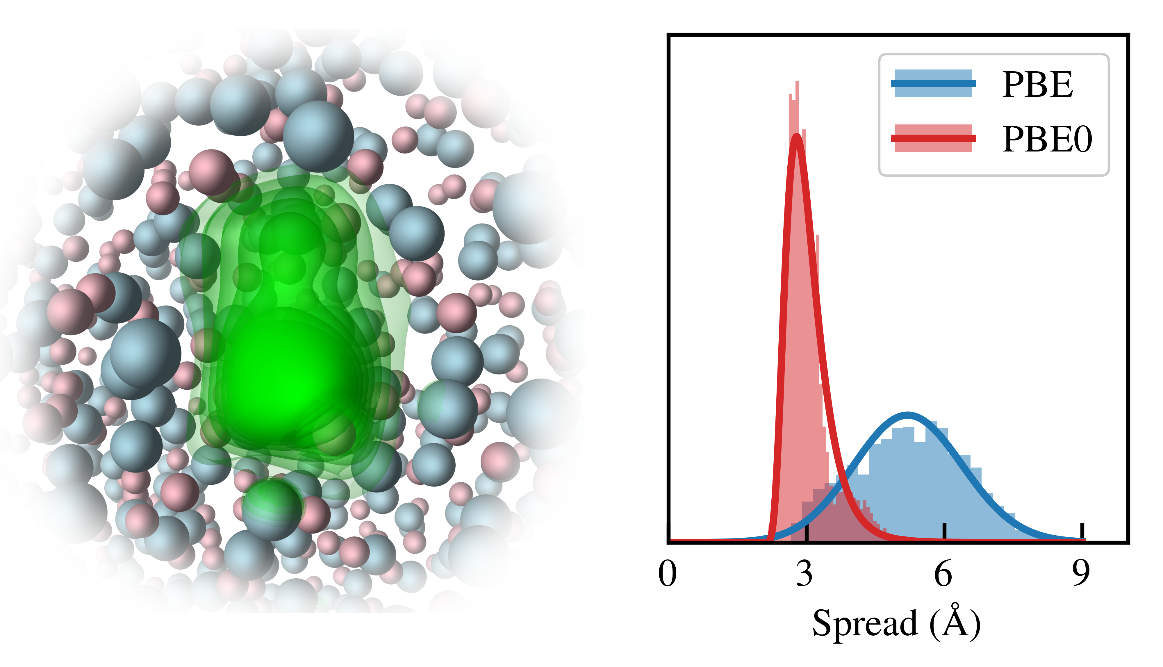
Figure 1: In the left panel, a typical snapshot taken from molecular dynamics simulations of non-stoichiometric molten NaCl. The volumetric data represents different isosurfaces of the bipolaron’s charge density. Pink spheres represent Na nuclei, while light blue spheres Cl nuclei. In the right panel, the distribution (normalized histogram) of the bipolaron’s spread computed with the PBE and the PBE0 functionals are reported in blue and red, respectively. The shaded bar-plots are the normalized histograms of the spread values; solid lines are log-normal fits to the histogram counts.

II Discussion

We study the non-stoichiometric molten salt $\mathrm{Na}_{1+x}\mathrm{Cl}_{1-x}$, with $x\approx 0.06$, and we compare its properties using two different functionals. The first, chosen as our reference, is the semi-local PBE functional[35] that has been previously employed in ab initio simulations of molten salts.[22] The second, hybrid, functional aims to enhance the localization of excess electrons. However, determining the appropriate amount of EXX to include in the calculation is often challenging. Advanced techniques have been developed to determine the optimal EXX fraction, able to provide an accurate description of excess electrons, especially polarons, in materials. These techniques involve approaches such as enforcing piecewise linearity on the DFT energy with respect to electron occupation, addressing in this way the self-interaction errors of DFT.[36, 37] Here, we have instead chosen to employ the widely-used PBE0 formulation,[38] which is parameter-free and features 25% of EXX. We have found this fraction of EXX to be sufficient to induce a suitable level of localization of the excess electrons that allow us to qualitatively compare the differences in properties of non-stoichiometric molten salts under the influence of EXX.

We focus on the simple case of 33 Na atoms and 31 Cl atoms. Simulations employing both functionals are carried out in a cubic cell with a side of $13\,\text{\r{A}}$ at a density of $1.40\,\mathrm{g/cm^{3}}$ and a temperature of $1300\,\mathrm{K}$. Further information is provided in Appendix B. The presence of two extra Na atoms with respect to the stoichiometric formula leads to ionization and the release of one electron each, forming a solvated electronic pair called bipolaron.[3, 4, 5, 21, 22, 28, 39] The Highest Occupied Molecular Orbital (HOMO) corresponds to the bipolaron’s wavefunction.[22, 28] To comprehend the bipolaron’s characteristics, we determine the location and spatial extent of the HOMO. This can be achieved by transforming the Kohn-Sham Bloch states into a localized basis, such as the Wannier Functions (WFs). We can thus determine Wannier Centers (WCs) and Spreads (WSs), where the WS quantifies the spatial extent of the orbitals. In particular, the HOMO WC represents the bipolaron’s position, while the HOMO WS provides insights into its degree of localization.[31, 40, 22] We employ the widely used Maximally Localized Wannier Functions (MLWFs)[40], where the HOMO WS is defined as the variance of the position operator evaluated over the HOMO WF. In the following, we will loosely speak of spread referring also to its square root which, having the dimensions of a length, facilitates comparisons with distances.

A typical snapshot taken from a simulation of non-stoichiometric molten NaCl is shown in the left panel of Fig. 1, where several isosurfaces of the HOMO charge density are colored in green. In the right panel, we show the distribution of the HOMO WSs computed during the two simulations. Here, it is worth mentioning that the MLWF construction may underestimate the WS when the latter is not small compared to the simulation box size,[41] as it occurs when EXX is not considered. Therefore, the difference in the WS distribution between PBE and PBE0 may be even amplified, should the WS be estimated according to the accurate formulation of Ref. 41. Including a portion of EXX in the XC functional impacts both structural and dynamical properties of non-stoichiometric NaCl. In the subsequent sections, we will address these aspects.

II.1 Structural properties

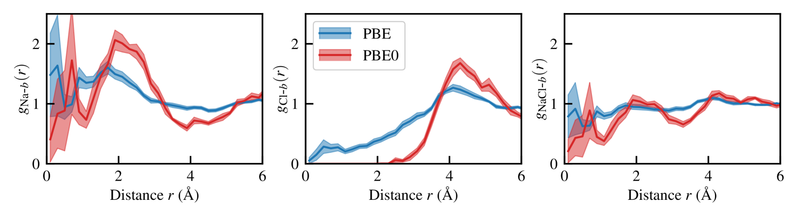
Figure 2: RPDFs of the bipolaron with Na (left), Cl (middle), and both (right), both with and without EXX. The shaded areas represent standard deviations obtained via a block average of $2.5\,\mathrm{ps}$-long segments of trajectory.

To understand the structural effects of adding the EXX to the XC functional, we compute the Radial Pair Distribution Function (RPDF), $g(r)$, of the bipolaron (hereon labeled by $b$) and the atomic species in NaCl, that are shown in Fig. 2. We observe several distinct features that reveal the differences between PBE and PBE0. First, the likelihood of locating a Cl ion in close proximity to the bipolaron is significantly lower in the case of PBE0 as compared to PBE. Second, RPDF for the interaction between the bipolaron and any ion exhibits a much more pronounced structure with PBE0. This indicates the existence of a well-defined shell structure surrounding, on average, the bipolaron, which is notably absent when using the PBE functional. In contrast, PBE predicts a comparatively uniform distribution of ions around the bipolaron, lacking any discernible shell-like organization. It must be noted that size effects can affect the results at large distances, since the RPDFs have not completely decayed within half the simulation cell’s size. Features at shorter distances are nonetheless significantly different for PBE and PBE0.

Since incorporating a fraction of EXX affects both the bipolaron’s spread distribution (see the right panel of Fig. 1) and its local environment (see Fig. 2), we investigated the potential correlation between electronic and structural properties. To this end, we calculated the time-correlation functions of the (square root of the) bipolaron’s spread, $\varsigma$, and the distance of the first peak in the instantaneous partial RPDF between the bipolaron and Na ions, $r_{\mathrm{peak}}$, which we use as a proxy for the bipolaron’s local environment. The results are reported in Fig. 3. The time-correlation functions were calculated using standardized time-series data for the spread and $r_{\mathrm{peak}}$, according to:

$$C_{AB}(t)=\frac{\left\langle(A(t)-\langle A\rangle)(B(0)-\langle B\rangle)\right\rangle}{\sqrt{\left\langle(A-\langle A\rangle)^{2}\right\rangle\left\langle(B-\langle B\rangle)^{2}\right\rangle}},$$ (1)

with $A$ and $B$ being $\varsigma$ or $r_{\mathrm{peak}}$. The characteristic $\varsigma$–$\varsigma$ and $r_{\mathrm{peak}}$–$r_{\mathrm{peak}}$ correlation times appear to be the same for the PBE0 functional. For PBE, instead, the correlation time of $r_{\mathrm{peak}}$ is shorter than that of the spread, likely due to the fact that the erratic motion of the bipolaron in the presence of a semi-local functional make its local environment rapidly change in time. The cross-correlation function is relatively small in both cases, suggesting that the two quantities are nearly uncorrelated with each other.

This analysis suggests that the effect of EXX can be fully understood only by examining average quantities sampled throughout the entire dynamics, rather than focusing on instantaneous values. This is in accordance with the fact that the distribution of the values of the spread—a statistical quantity—is markedly different in the two simulations, but the allowed values—instantaneous quantities—are partially overlapping. As a result, by evaluating a single snapshot it is almost impossible to discern whether the simulation was performed using a PBE or PBE0 functional. This is confirmed by a Principal Component Analysis (PCA) performed on Smooth Overlap of Atomic Positions (SOAP) descriptors [42, 43, 44, 45, 46] associated with the bipolaron’s local environments, whose results are presented in Appendix A.

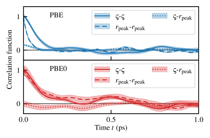
Figure 3: Time-correlation functions of the bipolaron’s spread, $\varsigma$, and the first peak in the instantaneous bipolaron-sodium RPDF, $r_{\mathrm{peak}}$. The shaded areas represent the standard errors on the means computed via block-averaging over $1\,\mathrm{ps}$-long segments of trajectory.

II.2 Transport properties

Charge transport in electronically insulating fluids relies on ionic motion. Allowing ions to move enables charge displacement. In the linear regime, the electrical conductivity, $\sigma$, can be expressed by the Green-Kubo (GK) formula:[47, 48, 49, 50, 51]

$$\sigma=\frac{\Omega}{3k_{B}T}\int_{0}^{\infty}\langle\mathbf{J}(t)\cdot\mathbf{J}(0)\rangle\differential{t},$$ (2)

or, equivalently, by the Helfand-Einstein formula:[52, 27]

$$\sigma=\frac{1}{3\Omega k_{\mathrm{B}}T}\lim_{t\to\infty}\frac{1}{2t}\langle\absolutevalue{\bm{\Delta\mu}(t)}^{2}\rangle.$$ (3)

Here, $\Omega$ represents the system’s volume, $k_{B}$ is Boltzmann’s constant, $T$ is the temperature, $\mathbf{J}$ denotes the charge flux, and $\bm{\Delta\mu}(t)=\Omega\int_{0}^{t}\mathbf{J}(t^{\prime})\differential{t^{\prime}}$ is the displaced dipole. For a quantum system in the adiabatic approximation, the definition of $\mathbf{J}$ must consider the quantum nature of electrons, while nuclei are treated as classical point charges. In principle, any partitioning of the continuous electronic charge density is equally valid. Within an independent-electron picture, $\mathbf{J}$ is usually defined in terms of either the macroscopic polarization[30] and its derivatives with respect to nuclear coordinates, the Born Effective-Charge tensors,[30, 53] or MLWFs.[40]

This perspective is quite different from the classical view of ionic fluids, where ions are considered point charges with a well-defined charge attached to them. This classical picture can be restored under suitable topological conditions by considering a combination of the gauge invariance of transport coefficients and Thouless’ theory of quantization of particle transport. This approach allows the use of a charge flux defined in terms of integer atomic Oxidation States (OSs):[26, 28]

$$\mathbf{J}(t)=\frac{e}{\Omega}\sum_{\ell=1}^{N}Q_{\ell}\mathbf{V}_{\ell}(t).$$ (4)

Here, $Q_{\ell}$ and $\mathbf{V}_{\ell}$ represent the OS and velocity of the $\ell$th nucleus, respectively. This holds when the topology of the configuration space of nuclear coordinates does not contain relevant regions where the electronic gap closes, and the system becomes metallic; a class of systems where this holds is that of stoichiometric molten salts.[26, 28] Conversely, when this condition is not met, charge is displaced not only as OSs attached to nuclei, but also through adiabatic electronic diffusion, as seen in the case of solvated electrons in molten salts.[22, 28] A classical picture can still be maintained from the perspective of MLWFs: in the Wannier representation, the charge flux becomes:

$$\mathbf{J}(t)=\frac{e}{\Omega}\left[\sum_{\ell=1}^{N}Z_{\ell}\mathbf{V}_{\ell}(t)-2\sum_{j=1}^{N_{\mathrm{el}}/2}\dot{\mathbf{R}}^{\mathrm{(W)}}_{j}\right],$$ (5)

where $\mathbf{R}_{j}^{(\mathrm{W})}$ refers to the position of the Wannier center associated with the $j$th occupied electronic band, and $Z_{\ell}$ is the nuclear (core) charge of the $\ell$th nucleus.[40, 54, 28]

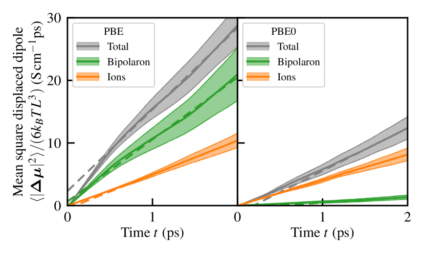
Figure 4: MSDD of non-stoichiometric molten NaCl computed with the PBE or the PBE0 functional. The shaded areas represent standard deviations on the mean computed via block averages.

It was shown in Refs. 22, 28 that, for the calculation of the electrical conductivity, we can employ the following (alternative) definition for the total charge flux:

$$\mathbf{J}(t)=\mathbf{J}_{\mathrm{ions}}(t)+\mathbf{J}_{b}(t),$$ (6)

where the flux assiociated to ions is $\mathbf{J}_{\mathrm{ions}}(t)\equiv\frac{e}{\Omega}\sum_{\ell=1}^{N}Q_{\ell}\mathbf{V}_{\ell}(t)$, and the one associated with the bipolaron is $\mathbf{J}_{b}(t)\equiv-2e\Omega^{-1}\dot{\mathbf{R}}_{\mathrm{HOMO}}^{\mathrm{(W)}}(t)$. In essence, here the charge flux is expressed as integer atomic OSs for the nuclei in the system, with $+1$ for Na ions and $-1$ for Cl ions (fist term at RHS), supplemented by the neutralizing effect of a solvated bipolaron with an “oxidation state” of $-2$ and a velocity corresponding to the time-derivative of the HOMO WC position (second term at RHS).[22] The corresponding displaced charge dipoles can be obtained by time integration of the charge fluxes, and then substituted in Eq. (3). The resulting total electrical conductivity is in general the sum:

$$\sigma=\sigma_{\mathrm{ions}}+\sigma_{b}+\sigma_{\mathrm{cross}}$$ (7)

where $\sigma_{\mathrm{cross}}\propto\int_{0}^{\infty}\langle\mathbf{J}_{\mathrm{ions}}(t)\cdot\mathbf{J}_{b}(0)\rangle\differential{t}$.

The expectation values appearing here, denoted by angled brackets, are estimated by block-averaging over trajectory segments and, within each block, via an average over initial times. This is implemented in the software analisi.[55] Fig. 4 displays the plot of the Mean Square Displaced Dipole (MSDD), ${(6L^{3}k_{\mathrm{B}}T)^{-1}\langle\absolutevalue{\bm{\Delta\mu}(t)}^{2}\rangle}$, as a function of time for various displaced dipoles related to the ions alone and to the bipolaron. The purely ionic contributions, whose slope are the respective values of $\sigma_{\mathrm{ions}}$, are comparable in both simulations. However, the bipolaron’s contribution, $\sigma_{b}$, in the PBE0 case is significantly smaller than that in the PBE simulation, where it played a leading role in determining the electrical conductivity value. In fact, the bipolaron diffusivity is reduced from $38\cdot 10^{-4}\,\mathrm{cm^{2}\,s^{-1}}$ for PBE to $3\cdot 10^{-4}\,\mathrm{cm^{2}\,s^{-1}}$ for PBE0, while the ionic diffusivity is of the order of $10^{-4}\,\mathrm{cm^{2}\,s^{-1}}$ in both cases. Despite the reduced bipolaron contribution due to the inclusion of EXX, the total conductivity is consistent with the sum of the ionic and bipolaronic contributions, as already demonstrated for PBE in non-stoichiometric KCl in Ref. 22 and confirmed here, thus showing the lack of correlation between the two. The total ionic conductivity is significantly reduced after the inclusion of EXX, going from $\sigma\approx 18\,\mathrm{S\,cm^{-1}}$ in the PBE case to $\sigma\approx 5\,\mathrm{S\,cm^{-1}}$ in the PBE0 case. The latter compares fairly well with experimental conductivity measurements on Na-NaCl melts at similar metal concentration,[2] while the former is appears rather overestimated.

To determine whether any form of dynamical correlation can exist, at least locally, we computed the cross-contribution to the conductivity between the bipolaron’s charge flux and a local ionic flux. The latter is defined as:

$$\mathbf{J}_{\mathrm{loc}}(\lambda,t)=\frac{e}{\Omega}\sum_{\ell=1}^{N}Q_{\ell}\mathbf{V}_{\ell}(t)\Theta(\lambda-|\mathbf{R}_{\ell}(t)-\mathbf{R}_{\mathrm{HOMO}}(t)|),$$ (8)

where $\Theta(x)$ is the Heaviside step-function, and $\lambda$ is some distance cutoff. Simply put, Eq. (8) contains the contribution to the charge flux due to ions within a distance $\lambda$ from the bipolaron, at each instant. A large value of $\lambda$ (up to half the simulation cell’s side) entails computing the entire ionic flux, while a small value of $\lambda$ yields a quantity that depends only on the neighborhood of the bipolaron’s position. The correlation between ionic and bipolaronic contributions to the electrical conductivity is estimated from the total local (i.e., $\lambda$-dependent) electrical conductivity, that we indicate with $\overline{\sigma}$ in order to distinguish it from the true electrical conductivity, $\sigma$. The local conductivity can be computed from Eq. (2) as

$$\overline{\sigma}(\lambda)\propto\int_{0}^{\infty}\langle(\mathbf{J}_{\mathrm{loc}}(\lambda,t)+\mathbf{J}_{b}(t))\cdot(\mathbf{J}_{\mathrm{loc}}(\lambda,0)+\mathbf{J}_{b}(0))\rangle\differential{t}.$$ (9)

Due to the relatively short PBE0 trajectories available, we employ the efficient cepstral analysis technique[56] as implemented in SporTran[57] to obtain the conductivity value from the fluxes’ time-series. Expanding the sums in the correlation function in Eq. (9) enables us to separate the contribution due to the bipolaron, $\sigma_{b}$, and the one due to the ions closest to it, $\sigma_{\mathrm{loc}}$, isolating the cross-correlation contribution between the two, $\sigma_{\mathrm{cross}}$:

$$\overline{\sigma}(\lambda)=\sigma_{b}+\sigma_{\mathrm{loc}}(\lambda)+\sigma_{\mathrm{cross}}(\lambda),$$ (10)

$$\sigma_{b}\propto\int_{0}^{\infty}\langle\mathbf{J}_{b}(t))\cdot\mathbf{J}_{b}(0)\rangle\differential{t},$$ (11)

$$\sigma_{\mathrm{loc}}(\lambda)\propto\int_{0}^{\infty}\langle\mathbf{J}_{\mathrm{loc}}(\lambda,t)\cdot\mathbf{J}_{\mathrm{loc}}(\lambda,0)\rangle\differential{t}.$$ (12)

Excluding $\sigma_{\mathrm{cross}}$ entails neglecting cross-correlation contributions between the ions and the bipolaron. The value of ${\sigma_{b}+\sigma_{\mathrm{loc}}}$ as a function of the ratio between $\lambda$ and the average Wannier spread of the bipolaron along the dynamics, $\varsigma_{\mathrm{avg}}$, is shown in Fig. 5. When $\lambda/\varsigma_{\mathrm{avg}}\ll 1$, $\mathbf{J}_{\mathrm{loc}}$ is small because only few to no ions are within the cutoff distance from the bipolaron, and $\sigma_{\mathrm{cross}}$ approaches zero, thus $\overline{\sigma}$ and ${\sigma_{b}+\sigma_{\mathrm{loc}}}$ are indistinguishable. Around $\lambda=\varsigma_{\mathrm{avg}}$, the local charge flux includes the contributions due to the ions that are closest to the bipolaron, and nothing else. Therefore, the correlation among the local charge flux and the bipolaron’s is maximal. When $\lambda$ is sufficiently large with respect to $\varsigma_{\mathrm{avg}}$ (i.e., $\lambda\gtrsim 1.5\varsigma_{\mathrm{avg}}$), correlation effects tend to vanish, as the local charge flux becomes equivalent to the global one. In fact, $\overline{\sigma}$ and ${\sigma_{b}+\sigma_{\mathrm{loc}}}$ become again compatible within error bars. The PBE0 results display a larger degree of correlation between ions and the bipolaron compared to the PBE ones: in fact, the relative difference between $\overline{\sigma}$ and ${\sigma_{b}+\sigma_{\mathrm{loc}}}$ becomes as large as $74\%$ for PBE0 at $\lambda=\varsigma_{\mathrm{avg}}$, while it stays at $19\%$ for PBE. Once again, this can be explained by the effect of EXX, that strengthens the interactions betwteen the ions and the bipolaron.

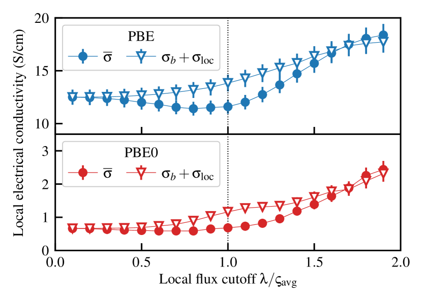
Figure 5: Local electrical conductivity of molten non-stoichiometric NaCl computed from the local charge flux of Eq. (8) as a function of the ratio between the local flux cutoff and the average bipolaron’s spread. Filled circles indicate bona fide GK results obtained from Eq. (9); empty triangles indicate the conductivity computed neglecting the correlation between the local ionic flux and the bipolaron’s motion. Note that the $y$-axis of the upper panel starts from $9\,\mathrm{S\,cm^{-1}}$.

III Conclusions

In this work, we have explored the impact of self-interaction on the structural and transport properties of dissolved electrons in non-stoichiometric molten salts through MD simulations of a binary NaCl melt with excess Na. We have found that, when EXX is taken into account, the bipolaron exhibits a tendency to localize within well-defined solvation cells, whereas the RPDF appears structureless when using a semi-local functional. The localization of the bipolaron in the solvation cell is manifested as a statistical property, rather than an instantaneous one, as the RPDFs computed separately on each step of the trajectory are uncorrelated with the bipolaron’s spatial extent, both statically and dynamically. The distribution of the bipolaron’s spread, entailing its spatial extension, testifies the larger average degree of localization in the PBE0 simulation, in accordance to the reduced self-interaction induced by the presence of EXX.

The implications of these observations on the ionic transport properties of the melt are substantial. Notably, the inclusion of EXX significantly decreases the electrical conductivity. On a local level, charge transport due to ions alone correlates with the bipolaron’s motion. This feat notwithstanding, this correlation dissipates on larger scales, resulting in a total electrical conductivity that can be decomposed into a purely ionic contribution, rationalized through integer and constant atomic OSs, and a purely bipolaronic contribution, associated with the motion of the WCs related to the HOMO.

Our study sheds light on the intricate interplay between charge and mass transport in non-stoichiometric molten salts, highlighting the importance of accurately accounting for self-interaction in simulations to capture the underlying mechanisms. By confirming the nontrivial regime where charge and mass transport are effectively uncorrelated, this work represents a first step towards further investigations into the fundamental processes governing the transport properties in complex fluids.

Data Availability

The data, sample input files, and data-analysis scripts that support the plots and relevant results within this paper are available on the Materials Cloud platform.[58] See DOI:https://doi.org/10.24435/materialscloud:8f-d7.

Author Declarations

The authors have no conflicts to disclose.

Appendix A Data-driven methods

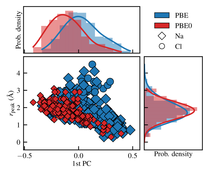
Figure 6: Correlation between the first PC of the bipolaron’s local environments and the the distance of the first peak of the instantaneous Na-$b$ RPDF. Diamond-shaped markers represent configurations where the closest ion is a sodium, while circles represent configuration where the closest ion is a chlorine.

The distinction between the two functionals is further emphasized by a principal component analysis (PCA) conducted to investigate the presence of clusters within the features characterizing the local atomic environments of the system.[46] To describe local environments we employed the widely used SOAP descriptors,[42, 43, 44] with parameters provided in Tab. 1, as implemented in librascal.[45] Snapshots were sampled every $100\,\mathrm{fs}$ to ensure data uncorrelation. The SOAP descriptors for all the considered local environments and for both functionals were collected into a single feature matrix, $[\mathbf{X}]_{e,f}$, where rows represent local environments and columns represent SOAP features. The matrix, $\mathbf{X}$, was subsequently centered, and its covariance matrix, ${\mathbf{C}=\mathbf{X}^{T}\mathbf{X}}$, was diagonalized with eigenvalues sorted in descending order. The PCA was then obtained by projecting $\mathbf{X}$ onto the first $n\mathrm{PC}$ eigenvectors of $\mathbf{C}$, thereby accounting for as much variance in $\mathbf{X}$ as possible while simultaneously reducing its dimensionality.

Fig. 6 illustrates the correlation between the first PC, which accounts for 17% of the variance, and the distance of the first peak of the instantaneous Na-$b$ RPDF, $r_{\mathrm{peak}}$. The Pearson correlation coefficients between these quantities for PBE and PBE0 are $-0.43$ and $-0.69$, respectively. Notably, the correlation for the PBE data gets to $-0.55$ when considering only structures where Na is the closest ion. This suggests that the first PC of the bipolaron’s SOAP descriptors is related to the ionic species and the proximity of its closest neighbor. The correlation is more robust for the PBE0 calculation, further corroborating the fact that the inclusion of EXX influences the first solvation shell of the bipolaron.

Keyword	Value
‘soap_type’	‘PowerSpectrum’
‘interaction_cutoff’	$6.5$
‘max_radial’	$12$
‘max_angular’	$10$
‘gaussian_sigma_constant’	$0.3$
‘gaussian_sigma_type’	‘Constant’
‘cutoff_smooth_width’	$0.5$
‘radial_basis’	‘GTO’
‘inversion_symmetry’	True
‘normalize’	True

Table 1: SOAP hyper-parameters used to conduct the PCA of the bipolaron’s local environments.

Appendix B Computational details

MD simulations are performed with the cp2k code,[59] version 9.1. The PBE and PBE0 functionals are parametrized according to the revised formulation also known as revPBE.[60] The electronic density is expanded in the TZV2P-GTH Gaussian basis set. We employed Gödecker-Teter-Hutter (GTH) pseudopotentials[61] encompassing electrons lying in the second shell, allowing for polarization effects which may contribute significantly to the accuracy of the simulations.[62] Gaussian functions are mapped to a multi-grid with four levels; the plane-wave cutoff for the finest level is set to $400\,\mathrm{Ry}$, with a relative cutoff of $60\,\mathrm{Ry}$. Computations are sped up with the Auxiliary Density Matrix Method (ADMM).[63] The hybrid calculations employ a Coulomb operator truncated[64] at $6\,\text{\AA}$ to further reduce the computational effort while retaining its accuracy. Long-range Van der Waals interactions are modeled through Grimme’s D3 corrections.[65] All calculations are spin-polarized in the singlet state, which is energetically favored. [22, 39]

Both MD simulations sample the canonical ensemble at $1300\,\mathrm{K}$ through the Bussi-Donadio-Parrinello thermostat[66] with a time constant of $1\,\mathrm{ps}$, i.e. two thousands times the integration time-step of $0.5\,\mathrm{fs}$. The Kohn-Sham wavefunctions are transformed to the basis of MLWFs [40] through Jacobi rotations every $1\,\mathrm{fs}$ to collect WCs and spreads to be used to compute the charge flux of Eq. (5). The PBE simulation has been thermalized for $5\,\mathrm{ps}$. The production run is $50\,\mathrm{ps}$ long. The PBE0 simulation has been initialized from a snapshot drawn from the equilibrated PBE simulation, and then further thermalized for $2\,\mathrm{ps}$. The production run is $15\,\mathrm{ps}$ long. Input files can be found in Materials Cloud.[58]

References

- Bredig, Johnson, and Smith Jr [1955] M. Bredig, J. Johnson, and W. T. Smith Jr, “Miscibility of liquid metals with salts. i. the sodium-sodium halide systems,” Journal of the American Chemical Society 77, 307–312 (1955).
- Bronstein and Bredig [1958] H. R. Bronstein and M. A. Bredig, “The electrical conductivity of solutions of alkali metals in their molten halides,” Journal of the American Chemical Society 80, 2077–2081 (1958).
- Selloni et al. [1987a] A. Selloni, R. Car, M. Parrinello, and P. Carnevali, “Electron pairing in dilute liquid metal-metal halide solutions,” The Journal of Physical Chemistry 91, 4947–4949 (1987a).
- Selloni et al. [1987b] A. Selloni, P. Carnevali, R. Car, and M. Parrinello, “Localization, hopping, and diffusion of electrons in molten salts,” Physical Review Letters 59, 823–826 (1987b).
- Fois et al. [1988] E. S. Fois, A. Selloni, M. Parrinello, and R. Car, “Bipolarons in metal-metal halide solutions,” The Journal of Physical Chemistry 92, 3268–3273 (1988).
- Selloni et al. [1989] A. Selloni, E. S. Fois, M. Parrinello, and R. Car, “Simulation of electrons in molten salts,” Physica Scripta T25, 261–267 (1989).
- Lindemann et al. [1983] G. Lindemann, R. Lassnig, W. Seidenbusch, and E. Gornik, “Cyclotron resonance study of polarons in GaAs,” Physical Review B 28, 4693–4703 (1983).
- Popp and Murray [1972] R. Popp and R. Murray, “Diffusion of the vk-polaron in alkali halides: Experiments in NaI and RbI,” Journal of Physics and Chemistry of Solids 33, 601–610 (1972).
- Chaikin, Garito, and Heeger [1972] P. M. Chaikin, A. F. Garito, and A. J. Heeger, “Excitonic polarons in molecular crystals,” Physical Review B 5, 4966–4969 (1972).
- Schindewolf [1968] U. Schindewolf, “Formation and properties of solvated electrons,” Angewandte Chemie International Edition in English 7, 190–203 (1968).
- Davy [1807] H. Davy, “I. the bakerian lecture, on some chemical agencies of electricity,” Philosophical Transactions of the Royal Society of London , 1–56 (1807).
- Marsalek et al. [2012] O. Marsalek, F. Uhlig, J. VandeVondele, and P. Jungwirth, “Structure, dynamics, and reactivity of hydrated electrons by ab initio molecular dynamics,” Accounts of Chemical Research 45, 23–32 (2012), pMID: 21899274, https://doi.org/10.1021/ar200062m .
- Buttersack et al. [2020] T. Buttersack, P. E. Mason, R. S. McMullen, H. C. Schewe, T. Martinek, K. Brezina, M. Crhan, A. Gomez, D. Hein, G. Wartner, et al., “Photoelectron spectra of alkali metal–ammonia microjets: From blue electrolyte to bronze metal,” Science 368, 1086–1091 (2020).
- Lan et al. [2021] J. Lan, V. Kapil, P. Gasparotto, M. Ceriotti, M. Iannuzzi, and V. V. Rybkin, “Simulating the ghost: quantum dynamics of the solvated electron,” Nature Communications 12, 766 (2021).
- Lan, Rybkin, and Pasquarello [2022] J. Lan, V. V. Rybkin, and A. Pasquarello, “Temperature dependent properties of the aqueous electron**,” Angewandte Chemie International Edition 61, e202209398 (2022), https://onlinelibrary.wiley.com/doi/pdf/10.1002/anie.202209398 .
- Bredig, Bronstein, and Smith [1955] M. A. Bredig, H. R. Bronstein, and W. T. J. Smith, “Miscibility of liquid metals with salts. ii. the potassium-potassium fluoride and cesium-cesium halide systems1,” Journal of the American Chemical Society 77, 1454–1458 (1955), https://doi.org/10.1021/ja01611a016 .
- Bredig and Johnson [1960] M. A. Bredig and J. W. Johnson, “Miscibility of metals with salts. v. the rubidium-rubidium halide systems,” The Journal of Physical Chemistry 64, 1899–1900 (1960), https://doi.org/10.1021/j100841a022 .
- Johnson and Bredig [1958] J. W. Johnson and M. A. Bredig, “Miscibility of metals with salts in the molten state. iii. the potassium-potassium halide systems,” The Journal of Physical Chemistry 62, 604–607 (1958), https://doi.org/10.1021/j150563a021 .
- Dworkin, Bronstein, and Bredig [1962] A. S. Dworkin, H. R. Bronstein, and M. A. Bredig, “Miscibility of metals with salts. v. the lithium-lithium halide systems,” The Journal of Physical Chemistry 66, 572–573 (1962), https://doi.org/10.1021/j100809a517 .
- Bredig [1963] M. Bredig, Mixtures of metals with molten salts (US Atomic Energy Commission, 1963).
- Fois, Selloni, and Parrinello [1989] E. Fois, A. Selloni, and M. Parrinello, “Approach to metallic behavior in metal–molten-salt solutions,” Physical Review B 39, 4812–4815 (1989).
- Pegolo, Grasselli, and Baroni [2020] P. Pegolo, F. Grasselli, and S. Baroni, “Oxidation states, thouless’ pumps, and nontrivial ionic transport in nonstoichiometric electrolytes,” Phys. Rev. X 10, 041031 (2020).
- Thouless [1983] D. J. Thouless, “Quantization of particle transport,” Phys. Rev. B 27, 6083–6087 (1983).
- Niu and Thouless [1984] Q. Niu and D. Thouless, “Quantised adiabatic charge transport in the presence of substrate disorder and many-body interaction,” Journal of Physics A: Mathematical and General 17, 2453 (1984).
- Marcolongo, Umari, and Baroni [2016] A. Marcolongo, P. Umari, and S. Baroni, “Microscopic theory and quantum simulation of atomic heat transport,” Nature Physics 12, 80–84 (2016).
- Grasselli and Baroni [2019] F. Grasselli and S. Baroni, “Topological quantization and gauge invariance of charge transport in liquid insulators,” Nature Physics 15, 967–972 (2019).
- Grasselli and Baroni [2021] F. Grasselli and S. Baroni, “Invariance principles in the theory and computation of transport coefficients,” The European Physical Journal B 94, 1–14 (2021).
- Pegolo, Baroni, and Grasselli [2022] P. Pegolo, S. Baroni, and F. Grasselli, “Topology, oxidation states, and charge transport in ionic conductors,” Annalen der Physik 534, 2200123 (2022).
- King-Smith and Vanderbilt [1993] R. King-Smith and D. Vanderbilt, “Theory of polarization of crystalline solids,” Physical Review B 47, 1651 (1993).
- Resta [1994] R. Resta, “Macroscopic polarization in crystalline dielectrics: the geometric phase approach,” Reviews of modern physics 66, 899 (1994).
- Resta and Sorella [1999] R. Resta and S. Sorella, “Electron localization in the insulating state,” Phys. Rev. Lett. 82, 370–373 (1999).
- Zhang and Yang [1998a] Y. Zhang and W. Yang, “A challenge for density functionals: Self-interaction error increases for systems with a noninteger number of electrons,” The Journal of chemical physics 109, 2604–2608 (1998a).
- Bao, Gagliardi, and Truhlar [2018] J. L. Bao, L. Gagliardi, and D. G. Truhlar, “Self-interaction error in density functional theory: An appraisal,” The Journal of Physical Chemistry Letters 9, 2353–2358 (2018).
- Sio et al. [2019] W. H. Sio, C. Verdi, S. Poncé, and F. Giustino, “Ab initio theory of polarons: Formalism and applications,” Phys. Rev. B 99, 235139 (2019).
- Perdew, Burke, and Ernzerhof [1996] J. P. Perdew, K. Burke, and M. Ernzerhof, “Generalized gradient approximation made simple,” Physical review letters 77, 3865 (1996).
- Falletta and Pasquarello [2022a] S. Falletta and A. Pasquarello, “Many-body self-interaction and polarons,” Phys. Rev. Lett. 129, 126401 (2022a).
- Falletta and Pasquarello [2022b] S. Falletta and A. Pasquarello, “Polarons free from many-body self-interaction in density functional theory,” Phys. Rev. B 106, 125119 (2022b).
- Adamo and Barone [1999] C. Adamo and V. Barone, “Toward reliable density functional methods without adjustable parameters: The PBE0 model,” The Journal of chemical physics 110, 6158–6170 (1999).
- Kristoffersen and Metiu [2018] H. H. Kristoffersen and H. Metiu, “Chemistry of solvated electrons in molten alkali chloride salts,” The Journal of Physical Chemistry C 122, 19603–19612 (2018).
- Marzari et al. [2012] N. Marzari, A. A. Mostofi, J. R. Yates, I. Souza, and D. Vanderbilt, “Maximally localized wannier functions: Theory and applications,” Reviews of Modern Physics 84, 1419 (2012).
- Li et al. [2023] K. Li, H.-Y. Ko, R. A. DiStasio Jr, and A. Damle, “An unambiguous and robust formulation for wannier localization,” arXiv preprint arXiv:2305.09929 (2023).
- Bartók, Kondor, and Csányi [2013] A. P. Bartók, R. Kondor, and G. Csányi, “On representing chemical environments,” Phys. Rev. B 87, 184115 (2013).
- De et al. [2016] S. De, A. P. Bartók, G. Csányi, and M. Ceriotti, “Comparing molecules and solids across structural and alchemical space,” Physical Chemistry Chemical Physics 18, 13754–13769 (2016).
- Musil et al. [2021a] F. Musil, A. Grisafi, A. P. Bartók, C. Ortner, G. Csányi, and M. Ceriotti, “Physics-inspired structural representations for molecules and materials,” Chemical Reviews 121, 9759–9815 (2021a).
- Musil et al. [2021b] F. Musil, M. Veit, A. Goscinski, G. Fraux, M. J. Willatt, M. Stricker, T. Junge, and M. Ceriotti, “Efficient implementation of atom-density representations,” The Journal of Chemical Physics 154, 114109 (2021b).
- Goscinski et al. [2021] A. Goscinski, G. Fraux, G. Imbalzano, and M. Ceriotti, “The role of feature space in atomistic learning,” Machine Learning: Science and Technology 2, 025028 (2021).
- Green [1952] M. S. Green, “Markoff random processes and the statistical mechanics of time-dependent phenomena.” J. Comp. Phys. 20, 1281–1295 (1952).
- Green [1954] M. S. Green, “Markoff random processes and the statistical mechanics of time-dependent phenomena. II. irreversible processes in fluids,” J. Comp. Phys. 22, 398–413 (1954).
- Kubo [1957] R. Kubo, “Statistical-mechanical theory of irreversible processes. I. General theory and simple applications to magnetic and conduction problems,” J. Phys. Soc. Japan 12, 570–586 (1957).
- Kubo, Yokota, and Nakajima [1957] R. Kubo, M. Yokota, and S. Nakajima, “Statistical-mechanical theory of irreversible processes. II. response to thermal disturbance,” J. Phys. Soc. Japan 12, 1203–1211 (1957).
- Baroni et al. [2020] S. Baroni, R. Bertossa, L. Ercole, F. Grasselli, and A. Marcolongo, “Heat transport in insulators from ab initio Green-Kubo theory,” in Handbook of Materials Modeling: Applications: Current and Emerging Materials, edited by W. Andreoni and S. Yip (Springer International Publishing, Cham, 2020) pp. 809–844.
- Helfand [1960] E. Helfand, “Transport coefficients from dissipation in a canonical ensemble,” Physical Review 119, 1 (1960).
- Ghosez, Michenaud, and Gonze [1998] P. Ghosez, J.-P. Michenaud, and X. Gonze, “Dynamical atomic charges: The case of AB O3 compounds,” Physical Review B 58, 6224 (1998).
- Resta [2021] R. Resta, “Faraday law, oxidation numbers, and ionic conductivity: The role of topology,” The Journal of Chemical Physics 155, 244503 (2021).
- Bertossa [2022] R. Bertossa, “analisi: your Swiss Army Knife of molecular dynamics analysis,” https://github.com/rikigigi/analisi (2022).
- Ercole, Marcolongo, and Baroni [2017] L. Ercole, A. Marcolongo, and S. Baroni, “Accurate thermal conductivities from optimally short molecular dynamics simulations,” Scientific reports 7, 15835 (2017).
- Ercole et al. [2022] L. Ercole, R. Bertossa, S. Bisacchi, and S. Baroni, “Sportran: A code to estimate transport coefficients from the cepstral analysis of (multivariate) current time series,” Computer Physics Communications 280, 108470 (2022).
- Talirz et al. [2020] L. Talirz, S. Kumbhar, E. Passaro, A. V. Yakutovich, V. Granata, F. Gargiulo, M. Borelli, M. Uhrin, S. P. Huber, S. Zoupanos, et al., “Materials cloud, a platform for open computational science,” Scientific data 7, 299 (2020).
- Hutter et al. [2014] J. Hutter, M. Iannuzzi, F. Schiffmann, and J. VandeVondele, “cp2k: atomistic simulations of condensed matter systems,” Wiley Interdisciplinary Reviews: Computational Molecular Science 4, 15–25 (2014).
- Zhang and Yang [1998b] Y. Zhang and W. Yang, “Comment on “generalized gradient approximation made simple”,” Phys. Rev. Lett. 80, 890–890 (1998b).
- Goedecker, Teter, and Hutter [1996] S. Goedecker, M. Teter, and J. Hutter, “Separable dual-space gaussian pseudopotentials,” Phys. Rev. B 54, 1703–1710 (1996).
- Ishii et al. [2015] Y. Ishii, S. Kasai, M. Salanne, and N. Ohtori, “Transport coefficients and the stokes–einstein relation in molten alkali halides with polarisable ion model,” Molecular Physics 113, 2442–2450 (2015), https://doi.org/10.1080/00268976.2015.1046527 .
- Guidon, Hutter, and VandeVondele [2010] M. Guidon, J. Hutter, and J. VandeVondele, “Auxiliary Density Matrix Methods for Hartree-Fock Exchange Calculations,” Journal of Chemical Theory and Computation 6, 2348–2364 (2010), pMID: 26613491.
- Spencer and Alavi [2008] J. Spencer and A. Alavi, “Efficient calculation of the exact exchange energy in periodic systems using a truncated coulomb potential,” Phys. Rev. B 77, 193110 (2008).
- Grimme et al. [2010] S. Grimme, J. Antony, S. Ehrlich, and H. Krieg, “A consistent and accurate ab initio parametrization of density functional dispersion correction (DFT-D) for the 94 elements H-Pu,” The Journal of chemical physics 132, 154104 (2010).
- Bussi, Donadio, and Parrinello [2007] G. Bussi, D. Donadio, and M. Parrinello, “Canonical sampling through velocity rescaling,” The Journal of chemical physics 126, 014101 (2007).