Utility Theory of Synthetic Data Generation

Abstract

Evaluating the utility of synthetic data is critical for measuring the effectiveness and efficiency of synthetic algorithms. Existing results focus on empirical evaluations of the utility of synthetic data, whereas the theoretical understanding of how utility is affected by synthetic data algorithms remains largely unexplored. This paper establishes utility theory from a statistical perspective, aiming to quantitatively assess the utility of synthetic algorithms based on a general metric. The metric is defined as the absolute difference in generalization between models trained on synthetic and original datasets. We establish analytical bounds for this utility metric to investigate critical conditions for the metric to converge. An intriguing result is that the synthetic feature distribution is not necessarily identical to the original one for the convergence of the utility metric as long as the model specification in downstream learning tasks is correct. Another important utility metric is model comparison based on synthetic data. Specifically, we establish sufficient conditions for synthetic data algorithms so that the ranking of generalization performances of models trained on the synthetic data is consistent with that from the original data. Finally, we conduct extensive experiments using non-parametric models and deep neural networks to validate our theoretical findings.

Keywords: Data Privacy, Generative Models, Utility Metrics, Learning Theory, Synthetic Data

1 Introduction

In recent years, there has been a growing interest in synthetic data generation due to its versatility in a wide range of applications, including financial data (Assefa et al.,, 2020; Dogariu et al.,, 2022) and medical data (Frid-Adar et al.,, 2018; Benaim et al.,, 2020; Chen et al.,, 2021). The core idea of data synthesis is generating a synthetic surrogate of the original dataset so that synthetic dataset can be used to replace or complement the original dataset for training and inference (Xing et al.,, 2022). For instance, synthetic data has enabled financial institutions to share their data while ensuring compliance with data sharing restrictions (Assefa et al.,, 2020). It has also been used to augment financial datasets for fraud detection purposes (Charitou et al.,, 2021; Cheng et al.,, 2023). Similarly, in the medical field, synthetic data has been utilized to improve data privacy and the performance of predictive models for disease diagnosis (Chen et al.,, 2021). In the literature, significant progress has been made in developing synthetic data algorithms, including classical marginal-based methods (McKenna et al.,, 2021; Zhang et al.,, 2021; Bi and Shen,, 2022; Li et al.,, 2023), generative adversarial networks (Hayes et al.,, 2017; Arjovsky et al.,, 2017; Goodfellow et al.,, 2020; Zhou et al.,, 2022), and diffusion models (Song et al.,, 2021; Ouyang et al.,, 2022). These synthetic data algorithms have demonstrated their superior performance in generating high-quality synthetic data for downstream training tasks (Jordon et al.,, 2019; Xie et al.,, 2018).

An important evaluation of synthetic data is the generalization ability of downstream tasks trained based on these synthetic data, i.e., utility. Specifically, we are interested in comparing statistical inferences and summaries derived from synthetic data with those from original data. For example, Karr et al., (2006) calculated the averaged overlap between the confidence intervals of coefficients estimated from synthetic and original data, while their standardized difference are adopted by Woo and Slavkovic, (2015) and Nowok et al., (2016) as a utility measure in linear regression. These utility metrics focus on the extent to which statistical results from synthetic data align with those from original data. Similar task-specific utility metrics have also been proposed for supervised learning, which involve comparing the generalization performance of models trained on synthetic and original data (Beaulieu-Jones et al.,, 2019; Hittmeir et al.,, 2019; Rankin et al.,, 2020; El Emam et al.,, 2021). Although many studies have proposed and evaluated utility metrics for synthetic data, theoretical understanding on the relationship between these metrics and the synthetic data algorithms is still lacking.

With this context, this paper aims to theoretically understand how a synthetic data algorithm affects the generalization performance of models learned from synthetic data, and explicates what properties a synthetic data algorithm should possess for generating a good synthetic dataset for a downstream learning task. We consider a common utility metric (Hittmeir et al.,, 2019; El Emam et al.,, 2021) used in existing empirical studies of synthetic data generation, which is defined as the absolute difference between the generalization errors on unobserved future data between the models estimated from original and synthetic datasets. The rationale behind this utility metric is that a good synthetic dataset should produce a model with comparable performance as the original dataset.

To study how synthetic data algorithms affect the behavior of the proposed utility metric, we establish explicit analytic bounds for the utility metrics in both regression (Theorem 1) and classification (Theorem 2). Specifically, the analytic bounds decompose the utility metrics into four major components, including the estimation error in the downstream learning task, the quality of synthetic features, the estimation of the regression function, and model specification in the downstream learning task. This decomposition enables us to identify key aspects that synthetic data algorithms should prioritize when generating high-quality synthetic datasets for downstream learning tasks.

There are two main theoretical findings from the analytic bounds regarding the convergence of the utility metrics. First, as long as synthetic features have perfect fidelity and the relationship between features and responses can be well approximated by synthetic data algorithms, the convergence of the utility metric to zero is guaranteed. The first result is expected since it is widely perceived that inferences from synthetic data will be valid if the distribution of synthetic data is not far from that of original data. Most importantly, the analytic bounds reveal an interesting phenomenon that if the model specification in the downstream learning task is correct in the sense that it can capture the relationship between features and responses, perfect feature fidelity is not a prerequisite for the convergence of utility metrics. This result shows that when the model specification is correct, the synthetic distribution is not required to be the same as the original distribution for producing a model with comparable generalization. This intriguing result contributes to our understanding of a surprising but frequently observed phenomenon: models trained on data in different contexts can still achieve competitive performance (Khan et al.,, 2019; Papadimitriou and Jurafsky,, 2020). For example, Papadimitriou and Jurafsky, (2020) verified that training models on non-linguistic data improves test performance on natural language. Our result suggests that the reason behind this phenomenon is due to the high approximation powers of the function classes of downstream tasks. This allows for training features from a different context to be used. To better demonstrate this interesting argument, we use linear regression as an illustrative example and establish the corresponding explicit convergence rate under imperfect feature fidelity (Theorem 3). Our simulation results for $K$-nearest neighbors (KNN; Coomans and Massart,, 1982), random forest regressor (RF; Breiman,, 2001), and deep neural networks (Farrell et al.,, 2021) empirically validate our theoretical findings, demonstrating that when the model specification is correct, the utility metrics converge to zero regardless of the disparity between synthetic and original features.

Another relevant but less stringent requirement for synthetic data is to obtain consistent model comparison results in the downstream tasks (Jordon et al.,, 2019, 2022). For example, consider releasing synthetic data for data competitions such as Kaggle, synthetic data should allow practitioners achieve consistent model comparisons on the synthetic data. In other words, the relative performance of models trained on synthetic data should be consistent with that on original data. Therefore, this paper also delves into exploring the conditions for synthetic data to maintain consistent results when comparing models during downstream learning tasks. To this end, we propose a new metric called $(V,d)$-fidelity level to measure distribution difference between original and synthetic features. Specifically, we show that consistent model comparison is achievable on synthetic data (Theorem 4) as long as the generalization gap between two model classes is large enough to neutralize the dissimilarity between distributions of synthetic and original features (Assumption 5). To the best of our knowledge, our work provides the first analytic solution to the question posed in Jordon et al., (2022) about when the relative performance of models estimated from synthetic data is consistent with that of original data.

The remainder of the paper is organized as follows. We first introduce necessary notations. In Section 2, we present background information and basic concepts related to supervised learning. In Section 3, we introduce the data synthesis framework and utility metrics for supervised learning considered in this paper. Section 4 establishes analytic bounds for the utility metrics and provides explicit sufficient conditions for their convergence. In Section 5, we present several examples that illustrate the asymptotic behavior of the utility metrics under different conditions. We also apply the analytic bounds to study the convergence of the utility metrics in linear regression. In Section 6, we study the sufficient conditions of synthetic data to yield consistent results as original data in comparing performances of different models. In Section 7, we conduct extensive simulations and a real-world application to support our theoretical results. Finally, the Appendix contains auxiliary results and the proofs of theoretical results in this paper.

Notation: For a vector $\bm{x}\in\mathbb{R}^{p}$, we denote its $l_{1}$-norm and $l_{2}$-norm as $\|\bm{x}\|_{1}=\sum_{i=1}^{p}|x_{i}|$ and $\|\bm{x}\|_{2}=\big{(}\sum_{i=1}^{p}|x_{i}|^{2}\big{)}^{1/2}$, respectively. For a function $f:\mathcal{X}\rightarrow\mathbb{R}$, we denote its $L_{p}$-norm with respect to the probability measure $\mu$ as $\|f\|_{L^{p}(\mu)}=\big{(}\int_{\mathcal{X}}|f(\bm{x})|^{p}d\mu(\bm{x})\big{)}^{1/p}$. For two given sequences $\{A_{n}\}_{n\in\mathbb{N}}$ and $\{B_{n}\}_{n\in\mathbb{N}}$, we write $A_{n}\gtrsim B_{n}$ if there exists a constant $C>0$ such that $A_{n}\geq CB_{n}$ for any $n\in\mathbb{N}$. Additionally, we write $A_{n}\asymp B_{n}$ if $A_{n}\gtrsim B_{n}$ and $A_{n}\lesssim B_{n}$. For a random variable $X$, we let $\mathbb{P}_{X}(x)$ denote its density function at $x$ and $\mathbb{E}_{X}$ denote the expectation taken with respect to the randomness of $X$. For a sequence of random variable $\{X_{n}\}_{n\in\mathbb{N}}$, we let $X_{n}=o_{p}(1)$ represent that $X_{n}$ converges to 0 in probability.

2 Preliminaries

In supervised learning, there are two main types of problems: regression and classification. Let $\mathcal{D}_{r}=\{(\bm{x}_{i},y_{i})\}_{i=1}^{n}$ denote the typical dataset in regression problem, which are drawn from an unknown distribution of $(\bm{X},Y)$ with $\bm{X}\in\mathbb{R}^{p}$ and $Y$ is a scalar response. It is usually assumed that $y_{i}$’s are generated according to $y_{i}=\mu(\bm{x}_{i})+\epsilon_{i},i=1,\ldots,n$, where $\mu(\bm{x})=\mathbb{E}(Y|\bm{X}=\bm{x})$ is the conditional mean and $\epsilon_{i}$ is a noise term with mean 0 and variance $\sigma^{2}$. We denote the risk under the squared loss as $R_{s}(f)=\mathbb{E}\Big{[}\big{(}f(\bm{X})-Y\big{)}^{2}\Big{]}$, where the expectation is taken with respect to $(\bm{X},Y)$. We denote the excess risk as $\Phi_{s}(f)=R_{s}(f)-R_{s}(\mu)=\mathbb{E}\big{[}(f(\bm{X})-\mu(\bm{X}))^{2}\big{]}$. For a function class $\mathcal{F}$, we let $f_{\mathcal{F}}^{*}=\mathop{\mathrm{argmin}}_{f\in\mathcal{F}}R_{s}(f)$ denote the optimal function in $\mathcal{F}$ to minimize $R_{s}(f)$.

Let $\mathcal{D}_{c}=\{(\bm{x}_{i},z_{i})\}_{i=1}^{n}$ denote the dataset in binary classification, where $z_{i}$ takes values in $\{-1,1\}$ and

$$z_{i}=\begin{cases}1&\mbox{ with probability }\eta(\bm{x}_{i}),\\ -1&\mbox{ with probability }1-\eta(\bm{x}_{i}),\\ \end{cases}$$

where $\eta(\bm{x}_{i})=\mathbb{P}(Z=1|\bm{X}=\bm{x}_{i})$ and $Z$ denotes the response variable in classification. Denote the classification risk under the $0$-1 loss by $R_{0\mbox{-}1}(g)=\mathbb{E}\Big{[}I\big{(}\mathop{\mathrm{sign}}(g(\bm{X}))\neq Z\big{)}\Big{]}$, where $I(\cdot)$ is an indicator function. The optimal classifier minimizing $R_{0\mbox{-}1}(g)$ is the Bayes classifier, which is given as $g^{*}(\bm{X})=\mathop{\mathrm{sign}}\big{(}\eta(\bm{X})-1/2\big{)}$. The excess risk in classification is defined as

$$\Phi_{0\mbox{-}1}(g)=R_{0\mbox{-}1}(g)-R_{0\mbox{-}1}(g^{*})=\mathbb{E}\Big{[}I\big{(}\mathop{\mathrm{sign}}(g(\bm{X}))\neq g^{*}(\bm{X})\big{)}\big{|}2\eta(\bm{X})-1\big{|}\Big{]},$$

where the expectation is taken with respect to $\bm{X}$. For a function class $\mathcal{G}$, we let $g_{\mathcal{G}}^{*}=\mathop{\mathrm{argmin}}_{g\in\mathcal{G}}R_{0\text{-}1}(g)$ denote the optimal function in $\mathcal{G}$ to minimize $R_{0\text{-}1}(g)$.

The estimated models resulting from the regularized empirical risk minimization framework for regression and classification, respectively, are given as

$$\widehat{f}=\mathop{\mathrm{argmin}}_{f\in\mathcal{F}}\frac{1}{n}\sum_{i=1}^{n}\big{(}f(\bm{x}_{i})-y_{i}\big{)}^{2}+\lambda_{r}J_{r}(f),$$ (1)

$$\widehat{g}=\mathop{\mathrm{argmin}}_{g\in\mathcal{G}}\frac{1}{n}\sum_{i=1}^{n}\phi\big{(}\bm{x}_{i}z_{i}\big{)}+\lambda_{c}J_{c}(g),$$ (2)

where $\mathcal{F}$ is a class of functions for regression, $\mathcal{G}$ is a class of functions for classification, $\lambda_{r}$ and $\lambda_{c}$ are tuning parameters controlling the weight of the penalty term, $J_{r}(f)$ and $J_{c}(g)$ are two penalty terms, and $\phi$ is a margin loss for classification, such as hinge loss (Cortes and Vapnik,, 1995), logistic loss (Zhu and Hastie,, 2005), and $\psi$-loss (Shen et al.,, 2003).

3 Data Synthesis in Supervised Learning

In this paper, we consider a common framework for generating synthetic data for downstream learning tasks (Lin and Xu,, 2016; Yue et al.,, 2018; Bhattarai et al.,, 2020). As illustrated in Figure 1, the generation process involves two stages: feature generation and response generation. A feature generator $G$ is used to generate synthetic features based on a set of original features, and the resulting synthetic features are denoted as $\{\widetilde{\bm{x}}_{i}\}_{i=1}^{\widetilde{n}}$, where $\widetilde{n}$ is the size of the synthetic dataset. Various methods can be used for feature generation, such as generative adversarial networks (GANs; Goodfellow et al.,, 2014; Xu et al.,, 2019), re-sampling techniques (Aggarwal and Philip,, 2008), and copula methods (Wan et al.,, 2019). Once the synthetic features are generated, responses are generated using an estimation model, which aims to capture the functional relationship between the features and responses, such as non-parametric methods (Ho,, 1995; Breiman,, 2001; Györfi et al.,, 2002; Hall et al.,, 2008) and deep learning models (Hornik et al.,, 1989). We let $\widehat{\mu}$ and $\widehat{\eta}$ denote the estimators of $\mu$ and $\eta$ in regression and classification, respectively. After estimating this relationship, we then generate responses such that they are comparable to those from the original dataset.

Specifically, synthetic responses for regression and classification are generated as

$$\text{Regression: }\widetilde{y}_{i}=\widehat{\mu}(\widetilde{\bm{x}}_{i})+\widetilde{\epsilon}_{i}\mbox{ and }\text{Classification: }\widetilde{z}_{i}=\begin{cases}1\mbox{ with probability }\widehat{\eta}(\widetilde{\bm{x}}_{i}),\\ -1\mbox{ with probability }1-\widehat{\eta}(\widetilde{\bm{x}}_{i}),\\ \end{cases}$$

respectively, where $\widetilde{\epsilon}_{i}$ denotes a noise term with mean 0 and finite variance.

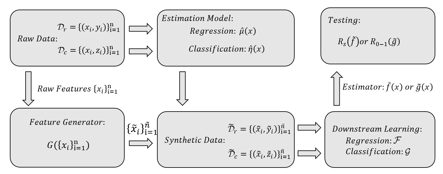
Figure 1: The architecture for generating and evaluating synthetic data in supervised learning.

Let $\widetilde{\mathcal{D}}_{r}=\{(\bm{\widetilde{x}}_{i},\widetilde{y}_{i})\}_{i=1}^{\widetilde{n}}$ and $\widetilde{\mathcal{D}}_{c}=\{(\bm{\widetilde{x}}_{i},\widetilde{z}_{i})\}_{i=1}^{\widetilde{n}}$ be synthetic datasets generated based on $\mathcal{D}_{r}$ and $\mathcal{D}_{c}$, respectively. Accordingly, we define the estimated models in regression and classification based on synthetic datasets as

$$\widetilde{f}=\mathop{\mathrm{argmin}}_{f\in\mathcal{F}}\frac{1}{\widetilde{n}}\sum_{i=1}^{\widetilde{n}}\big{(}f(\widetilde{\bm{x}}_{i})-\widetilde{y}_{i}\big{)}^{2}+\lambda_{r}J_{r}(f),$$ (3)

$$\widetilde{g}=\mathop{\mathrm{argmin}}_{g\in\mathcal{G}}\frac{1}{\widetilde{n}}\sum_{i=1}^{\widetilde{n}}\phi\big{(}g(\widetilde{\bm{x}}_{i})\widetilde{z}_{i}\big{)}+\lambda_{c}J_{c}(g).$$ (4)

The central problem of data synthesis in supervised learning is whether $\widetilde{f}$ (or $\widetilde{g}$) performs similarly to $\widehat{f}$ (or $\widehat{g}$) in terms of generalization (Hittmeir et al.,, 2019; Rankin et al.,, 2020). In other words, the performance of estimators trained on the synthetic dataset should be comparable to those trained on the original dataset (Jordon et al.,, 2019). Motivated by this, we consider a common evaluation metric to measure the utility of synthetic datasets for both regression and classification,

$$U_{r}(\widetilde{f},\widehat{f})=\Big{|}R_{s}(\widetilde{f})-R_{s}(\widehat{f})\Big{|}\mbox{ and }U_{c}(\widetilde{g},\widehat{g})=\Big{|}R_{0\text{-}1}(\widetilde{g})-R_{0\text{-}1}(\widehat{g})\Big{|}.$$ (5)

The rationale behind $(\ref{UtiR})$ is that the regression/classification model trained from a synthetic dataset ought to possess similar performance in predicting unobserved samples (from real distribution) as that of the original dataset. Intuitively, the asymptotic behavior of $U_{r}(\widetilde{f},\widehat{f})$ and $U_{c}(\widetilde{g},\widehat{g})$ are affected by the difference between distributions of synthetic data and raw data. Take $U_{r}(\widetilde{f},\widehat{f})$ for example, when $\mathcal{D}_{r}$ and $\widetilde{\mathcal{D}}_{r}$ are generated from the same distribution, the convergence of utility function is guaranteed by convergence of its the upper-bounding terms. Note that,

$$U_{r}(\widetilde{f},\widehat{f})\leq\Big{|}R_{s}(\widetilde{f})-R_{s}(f^{*}_{\mathcal{F}})\Big{|}+\Big{|}R_{s}(\widehat{f})-R_{s}(f^{*}_{\mathcal{F}})\Big{|},$$

where $f^{*}_{\mathcal{F}}=\mathop{\mathrm{argmin}}_{f\in\mathcal{F}}R(f)$ denotes the optimal function in $\mathcal{F}$ to approximate $\mu$. The right-hand side can be viewed as twice of the estimation errors in statistical learning theory, of which the convergence in probability is supported by a vast body of literature (Bartlett et al.,, 2006; Bousquet,, 2003; Vapnik,, 1999).

4 Utility Bounds

In this section, we establish upper bounds for the utility metrics defined in (5) to quantify how model specification ($\mathcal{F}$ or $\mathcal{G}$), estimation models ($\widehat{\mu}$ and $\widehat{\eta}$), and feature fidelity affect the convergence of $U_{r}(\widetilde{f},\widehat{f})$ and $U_{c}(\widetilde{g},\widehat{g})$. To measure the feature fidelity, we use the $\chi^{2}$-divergence, which characterizes the discrepancy between the underlying distributions of the original and synthetic features. Let $\widetilde{\bm{X}}$ denote the random variable of synthetic features. The $\chi^{2}$-divergence between $\bm{X}$ and $\widetilde{\bm{X}}$ is defined as:

$$\chi^{2}\big{(}\mathbb{P}_{\bm{X}}\|\mathbb{P}_{\widetilde{\bm{X}}}\big{)}=\int_{\mathcal{X}}\mathbb{P}_{\widetilde{\bm{X}}}(\bm{x})\left(\frac{\mathbb{P}_{\bm{X}}(\bm{x})}{\mathbb{P}_{\widetilde{\bm{X}}}(\bm{x})}-1\right)^{2}d\bm{x}.$$

The $\chi^{2}$-divergence, belonging to a general family of discrepancy measures for distributions called $f$-divergences (Rényi,, 1961), is commonly used to measure the association between two distributions in the domain of synthetic data generation (Mao et al.,, 2017; Tao et al.,, 2018; Ghosh et al.,, 2018; Mireshghallah et al.,, 2022).

Assumption 1.

Assume that the synthetic distribution is constructed appropriately such that $\chi^{2}\big{(}\mathbb{P}_{\bm{X}}\|\mathbb{P}_{\widetilde{\bm{X}}}\big{)}<\infty$.

The Assumption 1 is very mild in the sense that it only requires the $\chi^{2}$-divergence between the distributions of $\bm{X}$ and $\widetilde{\bm{X}}$ to be finite. Empirically, $\chi^{2}$-divergence is also widely used as an objective function in GANs for generating synthetic data (Mao et al.,, 2017; Tao et al.,, 2018).

Utility Bound for Regression: Let $\widetilde{Y}$ denote the random variable of the synthetic responses $\{\widetilde{y}_{i}\}_{i=1}^{\widetilde{n}}$. For regression, we define the risk and the excess risk under the synthetic distribution as

$$\widetilde{R}_{s}(f)=\mathbb{E}\Big{[}\big{(}f(\widetilde{\bm{X}})-\widetilde{Y}\big{)}^{2}\Big{]}\mbox{ and }\widetilde{\Phi}_{s}(f)=\mathbb{E}\Big{[}\big{(}f(\widetilde{\bm{X}})-\widehat{\mu}(\widetilde{\bm{X}})\big{)}^{2}\Big{]},$$

respectively, where the expectation is taken with respect to the randomness of $(\widetilde{\bm{X}},\widetilde{Y})$. Let $\widetilde{\Phi}_{s}(\widetilde{f}_{\mathcal{F}}^{*})=\mathop{\mathrm{argmin}}_{f\in\mathcal{F}}\widetilde{\Phi}_{s}(f)$ denote the optimal function in $\mathcal{F}$ to approximate $\widehat{\mu}$ under the synthetic distribution $\mathbb{P}_{\widetilde{\bm{X}},\widetilde{Y}}$.

Theorem 1.

Let $\widehat{f}$ and $\widetilde{f}$ be the functions defined in (1) and (3), respectively. Under Assumption 1, we have

$$U_{r}(\widetilde{f},\widehat{f})\leq \big{|}R_{s}(\widehat{f})-R_{s}(f^{*}_{\mathcal{F}})\big{|}+\big{|}\widetilde{R}_{s}(\widetilde{f})-\widetilde{R}_{s}(\widetilde{f}_{\mathcal{F}}^{*})\big{|}+2M\Upsilon_{1}\sqrt{\chi^{2}\big{(}\mathbb{P}_{\bm{X}}\|\mathbb{P}_{\widetilde{\bm{X}}}\big{)}}$$

$$+ 2\Upsilon_{2}\sqrt{\Phi_{s}(\widehat{\mu})}+4\Phi_{s}(\widehat{\mu}),$$ (6)

where $\Upsilon_{1}=\sqrt{\widetilde{\Phi}_{s}(\widetilde{f})}+2\sqrt{\widetilde{\Phi}_{s}(\widetilde{f}_{\mathcal{F}}^{*})}+\sqrt{\widetilde{\Phi}_{s}(f^{*}_{\mathcal{F}})}$, $\Upsilon_{2}=\sqrt{\Phi_{s}(\widetilde{f})}+2\sqrt{\Phi_{s}(\widetilde{f}_{\mathcal{F}}^{*})}+\sqrt{\Phi_{s}(f^{*}_{\mathcal{F}})}$, and $M$ satisfies $\max\{\|\widehat{\mu}\|_{L^{\infty}(\mathbb{P}_{\bm{X}})},\|\widetilde{f}\|_{L^{\infty}(\mathbb{P}_{\bm{X}})},\|\widetilde{f}_{\mathcal{F}}^{*}\|_{L^{\infty}(\mathbb{P}_{\bm{X}})},\|f_{\mathcal{F}}^{*}\|_{L^{\infty}(\mathbb{P}_{\bm{X}})}\}\leq M$.

Theorem 1 provides an upper bound for $U_{r}(\widetilde{f},\widehat{f})$, allowing us to specify sufficient conditions for the convergence of $U_{r}(\widetilde{f},\widehat{f})$. In statistical learning theory, the first term on the right-hand side of $(\ref{UUUR})$ is known as the estimation error, and its convergence in probability is generally assured under mild conditions about the entropy of $\mathcal{F}$ (Vapnik,, 1999; de Mello and Ponti,, 2018). The second term $\big{|}\widetilde{R}_{s}(\widetilde{f})-\widetilde{R}_{s}(\widetilde{f}_{\mathcal{F}}^{*})\big{|}$ represents the estimation error of $\widetilde{f}$ under the synthetic distribution. It is important to note that, $\big{|}\widetilde{R}_{s}(\widetilde{f})-\widetilde{R}_{s}(\widetilde{f}_{\mathcal{F}}^{*})\big{|}$ contains two sources of randomness from $\mathcal{D}_{r}$ and $\widetilde{\mathcal{D}}_{r}$, making $\big{|}\widetilde{R}_{s}(\widetilde{f})-\widetilde{R}_{s}(\widetilde{f}_{\mathcal{F}}^{*})\big{|}$ different from $\big{|}R_{s}(\widehat{f})-R_{s}(f^{*}_{\mathcal{F}})\big{|}$. With the convergence of the first two terms, we can draw two conclusions from Theorem 1. Firstly, when the feature generator produces synthetic features with perfect fidelity ($\chi^{2}\big{(}\mathbb{P}_{\bm{X}}\|\mathbb{P}_{\widetilde{\bm{X}}}\big{)}=0$), $U_{r}(\widetilde{f},\widehat{f})$ converges to zero as long as the estimation model $\widehat{\mu}$ approximates $\mu$ well, i.e., $\Phi_{s}(\widehat{\mu})=o_{p}(1)$ with the randomness from $\mathcal{D}_{r}$. Secondly, when the feature fidelity is not perfect, and $\chi^{2}\big{(}\mathbb{P}_{\bm{X}}\|\mathbb{P}_{\widetilde{\bm{X}}}\big{)}$ is bounded away from zero, the convergence of $U_{r}(\widetilde{f},\widehat{f})$ is guaranteed if $\Phi_{s}(\widehat{\mu})$ and $\Upsilon_{1}$ converge. In particular, the convergence of $\Upsilon_{1}$ is achieved when the regression model $\mu$ is correctly specified in the downstream regression task, with $\mu\in\mathcal{F}$. In this case, it can be verified that $\widetilde{\Phi}_{s}(f^{*}_{\mathcal{F}})=\|\widehat{\mu}-\mu\|_{L^{2}(\mathbb{P}_{\widetilde{\bm{X}}})}$. Furthermore, since $\widetilde{\Phi}_{s}(\widetilde{f}_{\mathcal{F}}^{*})\leq\widetilde{\Phi}_{s}(f^{*}_{\mathcal{F}})$ and $\widetilde{\Phi}_{s}(\widetilde{f})$ will converge to $\widetilde{\Phi}_{s}(\widetilde{f}_{\mathcal{F}}^{*})$ when unlimited synthetic samples are used for training, we can get the convergence of $\Upsilon_{1}$ by that of $\|\widehat{\mu}-\mu\|_{L^{2}(\mathbb{P}_{\widetilde{\bm{X}}})}$.

Utility Bound for Classification: Let $\widetilde{Z}$ denote the random variable of the synthetic responses $\{\widetilde{z}_{i}\}_{i=1}^{\widetilde{n}}$. For any $g$, we define its 0-1 risk and excess 0-1 risk under the synthetic distribution $\mathbb{P}_{\widetilde{\bm{X}},\widetilde{Z}}$ as

$$\widetilde{R}_{0\text{-}1}(g)=\mathbb{E}\Big{[}I\big{(}\mathop{\mathrm{sign}}\big{(}g(\widetilde{\bm{X}})\big{)}\neq\widetilde{Z}\big{)}\Big{]}\mbox{ and }\widetilde{\Phi}_{0\text{-}1}(g)=\mathbb{E}\Big{[}I\big{(}\mathop{\mathrm{sign}}\big{(}g(\widetilde{\bm{X}})\big{)}\neq\widetilde{g}^{*}(\widetilde{\bm{X}}\big{)}\cdot\big{|}2\widehat{\eta}(\widetilde{\bm{X}})-1\big{|}\Big{]},$$

respectively, where $\widetilde{g}^{*}(\bm{x})=\mathop{\mathrm{sign}}(\widehat{\eta}(\bm{x})-1/2))$.

Theorem 2.

Denote $\widetilde{g}_{\mathcal{G}}^{*}=\mathop{\mathrm{argmin}}_{g\in\mathcal{G}}\widetilde{R}_{0\text{-}1}(g)$ and $g_{\mathcal{G}}^{*}=\mathop{\mathrm{argmin}}_{g\in\mathcal{G}}R_{0\text{-}1}(g)$. Let $\widehat{g}$ and $\widetilde{g}$ be the functions defined in (2) and (4), respectively.

$$U_{c}(\widetilde{g},\widehat{g})\leq \big{|}R_{0\text{-}1}(\widehat{g})-R_{0\text{-}1}(g^{*}_{\mathcal{G}})\big{|}+\big{|}\widetilde{R}_{0\text{-}1}(\widetilde{g})-\widetilde{R}_{0\text{-}1}(\widetilde{g}^{*}_{\mathcal{G}})\big{|}+\Upsilon_{3}\sqrt{\chi^{2}\big{(}\mathbb{P}_{\bm{X}}\|\mathbb{P}_{\widetilde{\bm{X}}}\big{)}}$$

$$+ 2\|\widehat{\eta}-\eta\|_{L^{2}(\mathbb{P}_{X})}\Big{(}C(g^{*}_{\mathcal{G}})+2C(\widetilde{g}_{\mathcal{G}}^{*})+C(\widetilde{g})\Big{)}+4\Phi_{0\text{-}1}(\widehat{\eta}(\bm{x})-1/2),$$ (7)

where $C(g)=\sqrt{\mathbb{P}\big{(}g(\bm{X})(\widehat{\eta}(\bm{X})-1/2)<0\big{)}}$ and $\Upsilon_{3}=\sqrt{\widetilde{\Phi}_{0\text{-}1}(g^{*}_{\mathcal{G}})}+2\sqrt{\widetilde{\Phi}_{0\text{-}1}(\widetilde{g}^{*}_{\mathcal{G}})}+\sqrt{\widetilde{\Phi}_{0\text{-}1}(\widetilde{g})}$.

Similar to Theorem 1, we can obtain sufficient conditions for the convergence of $U_{c}(\widetilde{g},\widehat{g})$. The first two terms on the right-hand side of (2) are the estimation errors in classification under the true and synthetic distributions. It is straightforward to deduce that $\|\widehat{\eta}-\eta\|_{L^{2}(\mathbb{P}_{X})}$ and $\Phi_{0\text{-}1}(\widehat{\eta}(\bm{x})-1/2)$ both converge to 0 in probability as long as the estimation model $\widehat{\eta}$ can approximate $\eta$ well, which is achievable by some non-parametric models (Audibert and Tsybakov,, 2007). Furthermore, when feature fidelity is not perfect in sense that $\chi^{2}\big{(}\mathbb{P}_{\bm{X}}\|\mathbb{P}_{\widetilde{\bm{X}}}\big{)}$ is bounded away from zero, the convergence of $U_{c}(\widetilde{g},\widehat{g})$ entails the convergence of $\Upsilon_{3}$. Notice that $\widetilde{g}$ will converge to $\widetilde{g}^{*}_{\mathcal{G}}$ if unlimited synthetic samples are released for downstream learning and $\widetilde{\Phi}_{0\text{-}1}(\widetilde{g}^{*}_{\mathcal{G}})\leq\widetilde{\Phi}_{0\text{-}1}(g^{*}_{\mathcal{G}})$. Therefore, the convergence of $\Upsilon_{3}$ is achieved by requiring $\widetilde{\Phi}_{0\text{-}1}(g^{*}_{\mathcal{G}})$ close to zero. This requirement indicates that $\Phi_{0\text{-}1}(g)$ and $\widetilde{\Phi}_{0\text{-}1}(g)$ possess a similar minimizer in $\mathcal{G}$ and that $\mathcal{G}$ has a high approximation power for learning the relationship between features and responses. For example, $\widetilde{\Phi}_{0\text{-}1}(g^{*}_{\mathcal{G}})=O\left(\|\widehat{\eta}-\eta\|_{L^{2}(\mathbb{P}_{X})}\right)$ given that $g^{*}\in\mathcal{G}$ and that $\mathbb{P}_{\widetilde{\bm{X}}}(\bm{x})/\mathbb{P}_{\bm{X}}(\bm{x})$ is bounded (Audibert and Tsybakov,, 2007), which indicates that the convergence of $\|\widehat{\eta}-\eta\|_{L^{2}(\mathbb{P}_{X})}$ directly implies that of $\widetilde{\Phi}_{0\text{-}1}(g^{*}_{\mathcal{G}})$.

An intriguing finding is that achieving perfect feature fidelity during synthetic data generation is not always necessary for a downstream model estimated from synthetic data to generalize similarly to one trained on original data. Additionally, this discovery theoretically confirms a frequently observed phenomenon in extensive empirical studies, where models trained on data from a different context still show good generalization (Papadimitriou and Jurafsky,, 2020; Krishna et al.,, 2022).

5 Examples for Utility Metrics

In this section, we provide several examples to illustrate the theoretical results established in Section 4. Firstly, we provide a regression example to demonstrate that imperfect feature fidelity may result in a shift in optimality of generalization when the model specification is incorrect. That is, the generalization performance of a model trained from synthetic data may depend on the marginal distribution of synthetic features, and thus the convergence of the proposed utility metrics may not be achieved. However, if the model specification is accurate, the proposed utility metrics for both regression and classification can converge, indicating that perfect feature fidelity is not necessary when sharing synthetic data for supervised learning. Secondly, we will apply the analytical bounds derived in Section 4 to the linear regression to demonstrate the convergence of the proposed utility metrics even with imperfect feature fidelity. For linear regression, we provide the explicit form of its associated bound, and show that its convergence in probability under double asymptotics can be analytically derived. Additionally, similar results for the logistic regression is provided in Section S.1.2, where we verify the same theoretical insights.

5.1 Suboptimality with Imperfect Features

Theorems 1 and 2 demonstrate that the upper bounds established in the previous section do not converge if the model specification is inaccurate and the feature fidelity is imperfect ($\chi^{2}(\mathbb{P}_{\bm{X}}\|\mathbb{P}_{\widetilde{\bm{X}}})\neq 0$). In this section, we provide a toy example for regression to further illustrate that this phenomenon also applies to the utility metrics.

Consider the one-dimensional regression case and assume that $\mathcal{X}=[-1,1]$ and the regression function is $\mu(x)=|x|$. We assume that the observed responses are noise-free, that is $y=\mu(x)$. Furthermore, we assume that the true feature $X$ and the synthetic feature $\widetilde{X}$ follow the corresponding distributions:

$$\mathbb{P}_{X}(x)=1/2,x\in[-1,1]\mbox{ and }\mathbb{P}_{\widetilde{X}}(x)=\begin{cases}\alpha,&\mbox{ if }x\in[0,1],\\ 1-\alpha,&\mbox{ if }x\in[-1,0).\end{cases}$$ (8)

To simplify our analysis, we assume that the estimation model $\widehat{\mu}$ is identical to the true regression function $\mu(x)=|x|$. Moreover, we consider a scenario where there are infinitely many samples in both the true dataset and the synthetic dataset. This means that the estimated models $\widehat{f}$ and $\widetilde{f}$ can be obtained by minimizing the risks directly with $\lambda_{r}=0$.

Incorrect Model Specification: Under the model specification $\mathcal{F}=\{f(x)=\beta x:\beta\in\mathbb{R}\}$, the risks under the true and synthetic distributions are given as

$$R_{s}(f)=\frac{1+\beta^{2}}{3}\mbox{ and }\widetilde{R}_{s}(f)=\frac{\beta^{2}+(2-4\alpha)\beta+1}{3}.$$

The above calculations show that the estimated models can be obtained analytically as $\widehat{f}(x)=0$ and $\widetilde{f}(x)=(2\alpha-1)x$. Using these, $U_{r}(\widehat{f},\widetilde{f})$ can be computed as

$$U_{r}(\widehat{f},\widetilde{f})=\big{|}R_{s}(\widehat{f})-R_{s}(\widetilde{f})\big{|}=\frac{(2\alpha-1)^{2}}{3}>0,$$ (9)

for any $\alpha\in(0,1/2)\cup(1/2,1)$. The proposed utility metric in this case is always greater than 0 if $\mathbb{P}_{X}\neq\mathbb{P}_{\widetilde{X}}$ ($\alpha\neq 1/2$). This demonstrates that, in the case of an inaccurate model specification, the discrepancy between the true and synthetic distributions results in a gap between the generalization capabilities of models estimated from real and synthetic datasets. Such sub-optimality gap does not converge to zero even we have infinite samples.

Correct Model Specification: If the true model $\mu$ is correctly specified with $\mathcal{F}^{*}=\{f(x)=\beta|x|:\beta\in\mathbb{R}\}$, we have

$$R_{s}(f)=\frac{(1-\beta)^{2}}{3}\mbox{ and }\widetilde{R}_{s}(f)=\frac{(1-\beta)^{2}}{3}.$$

Clearly, the utility metric $U_{r}(\widehat{f},\widetilde{f})=0$ regardless of the value of $\alpha$ in $\mathbb{P}_{\widetilde{X}}$. This validates the second conclusion stated in Section 4 that perfect synthetic feature is not a prerequisite for the convergence of $U_{r}(\widehat{f},\widetilde{f})$ if the function class used in the downstream learning task is large enough to cover $\mu(x)$. Similarly, an example for classification is provided in Section S.1.1 for demonstrating the same phenomenon

5.2 Example: Linear Regression

This section provides an example using linear regression to illustrate the theoretical results presented in Section 4. The key point is that the convergence of $U_{r}(\widetilde{f},\widehat{f})$ does not require perfect feature fidelity, as long as the regression function $\mu$ is correctly specified. To simplify the analysis, we assume that the synthetic features are sampled from a fixed distribution $\mathbb{P}_{\widetilde{\bm{X}}}$ that is independent of $\{\bm{x}_{i}\}_{i=1}^{n}$. We also assume that the distributions of the original features $\mathbb{P}_{\bm{X}}$ and the synthetic features $\mathbb{P}_{\widetilde{\bm{X}}}$ satisfy Assumption 2. This assumption considers a scenario where all coordinates of $\bm{X}$ and $\widetilde{\bm{X}}$ are independent, and they follow different distributions, indicating that $\chi(\mathbb{P}_{\bm{X}}\|\mathbb{P}_{\widetilde{\bm{X}}})\neq 0$.

Assumption 2.

For the random feature vectors $\bm{X}=(X_{1},\ldots,X_{p})$ and $\widetilde{\bm{X}}=(\widetilde{X}_{1},\ldots,\widetilde{X}_{p})$, we assume that (1) $X_{i}\perp\!\!\!\perp\widetilde{X}_{i}$ with $\mathbb{E}(X_{i})=\mathbb{E}(\widetilde{X}_{i})=0$, $\text{Var}(X_{i})=\lambda_{i}$, and $\text{Var}(\widetilde{X}_{i})=\widetilde{\lambda}_{i}$ for $i=1,\ldots,p$ (2) $X_{i}\perp\!\!\!\perp X_{j}$ and $\widetilde{X}_{i}\perp\!\!\!\perp\widetilde{X}_{j}$ for any $i\neq j$.

For the observed dataset $\mathcal{D}_{r}=\{(\bm{x}_{i},y_{i})\}_{i=1}^{n}$, we assume

$$y_{i}=\mu(\bm{x}_{i})+\epsilon_{i}=\bm{x}_{i}^{T}\bm{\beta}^{*}+\epsilon_{i},$$ (10)

for $i=1,\ldots,n$, where $\bm{\beta}^{*}$ denotes the true coefficient vector. Furthermore, for the synthetic dataset $\widetilde{\mathcal{D}}_{r}=\{(\widetilde{\bm{x}}_{i},\widetilde{y}_{i})\}_{i=1}^{\widetilde{n}}$, we assume the generation of the synthetic response $\widetilde{y}_{i}$ employs the ordinal least squares (OLS) estimator.

$$\widetilde{y}_{i}=\widehat{\mu}(\widetilde{\bm{x}}_{i})+\widetilde{\epsilon}_{i}=\widehat{\bm{\beta}}^{T}\widetilde{\bm{x}}_{i}+\widetilde{\epsilon}_{i},$$ (11)

for $i=1,\ldots,\widetilde{n}$, where $\widehat{\bm{\beta}}=(\mathbb{X}^{T}\mathbb{X})^{-1}\mathbb{X}^{T}\mathbb{Y}$, $\mathbb{X}=(\bm{x}_{1},\bm{x}_{2},\ldots,\bm{x}_{n})^{T}$, $\mathbb{Y}=(y_{1},y_{2},\ldots,y_{n})^{T}$, and $\widetilde{\epsilon}_{i}$ is bounded synthetic noise with variance $\widetilde{\sigma}^{2}$.

In the downstream regression task, we assume that the model specification is correct, that is $\mathcal{F}=\{f(\bm{x})=\bm{\beta}^{T}\bm{x}:\bm{\beta}\in\mathbb{R}^{p}\}$. With this, the estimated models based on $\mathcal{D}_{r}=\{(\bm{x}_{i},y_{i})\}_{i=1}^{n}$ and $\widetilde{\mathcal{D}}_{r}=\{(\widetilde{\bm{x}}_{i},\widetilde{y}_{i})\}_{i=1}^{\widetilde{n}}$, respectively, are given as

$$\widehat{f}_{LR}(\bm{x})=\bm{x}^{T}(\mathbb{X}^{T}\mathbb{X})^{-1}\mathbb{X}^{T}\mathbb{Y}\mbox{ and }\widetilde{f}_{LR}(\bm{x})=\bm{x}^{T}(\widetilde{\mathbb{X}}^{T}\widetilde{\mathbb{X}})^{-1}\widetilde{\mathbb{X}}^{T}\widetilde{\mathbb{Y}},$$

where $\widetilde{\mathbb{X}}=(\widetilde{\bm{x}}_{1},\widetilde{\bm{x}}_{2},\ldots,\widetilde{\bm{x}}_{\widetilde{n}})^{T}$ and $\widetilde{\mathbb{Y}}=(\widetilde{y}_{1},\widetilde{y}_{2},\ldots,\widetilde{y}_{\widetilde{n}})^{T}$.

Assumption 3.

Assume that $\widetilde{\mathbb{X}}^{T}\widetilde{\mathbb{X}}$ and $\mathbb{X}^{T}\mathbb{X}$ are both invertible almost surely.

Theorem 3.

Denote that $\bm{\Lambda}={\rm diag}(\lambda_{1},\ldots,\lambda_{p})$ and $\widetilde{\bm{\Lambda}}={\rm diag}(\widetilde{\lambda}_{1},\ldots,\widetilde{\lambda}_{p})$. Under Assumptions 1-3, the analytic bound established in Theorem 1 becomes

$$U_{r}( \widehat{f}_{LR},\widetilde{f}_{LR})\leq 13\text{trace}\Big{(}\bm{\epsilon}\bm{\epsilon}^{T}\mathbb{Q}\bm{\Lambda}\mathbb{Q}^{T}\Big{)}+\text{trace}\Big{(}\widetilde{\bm{\epsilon}}\widetilde{\bm{\epsilon}}^{T}\widetilde{\mathbb{Q}}\widetilde{\bm{\Lambda}}\widetilde{\mathbb{Q}}^{T}\Big{)}$$

$$+2M_{LR}\chi^{2}\left(\mathbb{P}_{\bm{X}}\|\mathbb{P}_{\widetilde{\bm{X}}}\right)\left\{\sqrt{\text{trace}\Big{(}\widetilde{\bm{\epsilon}}\widetilde{\bm{\epsilon}}^{T}\widetilde{\mathbb{Q}}\widetilde{\bm{\Lambda}}\widetilde{\mathbb{Q}}^{T}\Big{)}}+\sqrt{\text{trace}\Big{(}\bm{\epsilon}\bm{\epsilon}^{T}\mathbb{Q}\widetilde{\bm{\Lambda}}\mathbb{Q}^{T}\Big{)}}\right\}$$

$$+\sqrt{2\text{trace}\Big{(}\bm{\epsilon}\bm{\epsilon}^{T}\mathbb{Q}\widetilde{\bm{\Lambda}}\mathbb{Q}\Big{)}}\sqrt{\text{trace}\Big{(}\bm{\epsilon}\bm{\epsilon}^{T}\mathbb{Q}\bm{\Lambda}\mathbb{Q}^{T}\Big{)}},$$ (12)

where $\mathbb{Q}=\mathbb{X}\big{(}\mathbb{X}^{T}\mathbb{X})^{-1}$, $\widetilde{\mathbb{Q}}=\widetilde{\mathbb{X}}\big{(}\widetilde{\mathbb{X}}^{T}\widetilde{\mathbb{X}})^{-1}$, $M_{LR}=\max\left\{\sup_{\bm{x}\in\mathcal{X}}\big{|}\bm{x}^{T}\mathbb{Q}^{T}\mathbb{Y}\big{|},\sup_{\bm{x}\in\mathcal{X}}\big{|}\bm{x}^{T}\widetilde{\mathbb{Q}}^{T}\widetilde{\mathbb{Y}}\big{|}\right\}$, $\text{trace}(\cdot)$ is the trace of a matrix, $\bm{\epsilon}=(\epsilon_{1},\ldots,\epsilon_{n})^{T}$, and $\widetilde{\bm{\epsilon}}=(\widetilde{\epsilon}_{1},\ldots,\widetilde{\epsilon}_{\widetilde{n}})^{T}$. Furthermore, for any $\delta>0$, it holds that

$$\lim_{n\rightarrow\infty}\lim_{\widetilde{n}\rightarrow\infty}\mathbb{P}\Big{(}U_{r}(\widetilde{f}_{LR},\widehat{f}_{LR})>\delta\Big{)}=0,$$

where the randomness results from $\widetilde{\bm{\epsilon}}$, $\bm{\epsilon}$, $\mathbb{X}$, and $\widetilde{\mathbb{X}}$.

Theorem 3 shows that the utility metric $U_{r}(\widetilde{f}_{LR},\widehat{f}_{LR})$ converges to 0 when $n$ and $\widetilde{n}$ both increase to infinity regardless the difference between $\bm{X}$ and $\widetilde{\bm{X}}$ in distribution. This result suggests that even if the distributions of the original and synthetic features are different, models trained on these datasets can still perform similarly if the correct model specification is used. This is an important finding, as it implies that perfect feature fidelity is not necessary for effective synthetic data generation. This finding is consistent with our earlier conclusion in Section 4, implicitly indicating that the function class used in the downstream learning task is more important than feature fidelity for achieving good performance.

6 Model Comparison Based on Synthetic Data

Another application of synthetic data is for researchers to rank model performances simply based on synthetic data (Jordon et al.,, 2022). This requires that the ranking of model performances remains the same on both the synthetic and original data, which is particularly important when synthetic data is released for competitions, such as Kaggle. In the following, we present a formal definition for consistent model comparison based on synthetic data.

Definition 1.

(Consistent Model Comparison) Let $(\mathcal{F}_{1},\mathcal{F}_{2})$ or $(\mathcal{G}_{1},\mathcal{G}_{2})$ be a pair classes of models for comparison in the downstream learning task. We say the synthetic distribution $\mathbb{P}_{\widetilde{\bm{X}},\widetilde{Y}}$ or $\mathbb{P}_{\widetilde{\bm{X}},\widetilde{Z}}$ preserves the utility of consistent model comparison if

$$\mbox{Regression: }\Big{(}R_{s}(f_{\mathcal{F}_{1}}^{*})-R_{s}(f_{\mathcal{F}_{2}}^{*})\Big{)}\Big{(}R_{s}(\widetilde{f}_{\mathcal{F}_{1}}^{*})-R_{s}(\widetilde{f}_{\mathcal{F}_{2}}^{*})\Big{)}>0,$$

$$\mbox{Classification: }\Big{(}R_{0\text{-}1}(g_{\mathcal{G}_{1}}^{*})-R_{0\text{-}1}(g_{\mathcal{G}_{2}}^{*})\Big{)}\Big{(}R_{0\text{-}1}(\widetilde{g}_{\mathcal{G}_{1}}^{*})-R_{0\text{-}1}(\widetilde{g}_{\mathcal{G}_{2}}^{*})\Big{)}>0,$$

where $\widetilde{f}_{\mathcal{F}_{i}}^{*}=\mathop{\mathrm{argmin}}_{f\in\mathcal{F}_{i}}\widetilde{R}_{s}(f)$ and $\widetilde{g}_{\mathcal{G}_{i}}^{*}=\mathop{\mathrm{argmin}}_{g\in\mathcal{G}_{i}}\widetilde{R}_{0\text{-}1}(g)$ for $i=1,2$.

Particularly, when the synthetic and original distributions are identical, the optimal models will necessarily be the same. As a result, it is straightforward to derive a consistent model comparison based on synthetic data. However, more interestingly, consistent model comparison can still be achieved using synthetic data even if the synthetic and original distributions are not identical. To illustrate this phenomenon, we provide an intuitive example in Figure 2. In this example, we assume that $f_{\mathcal{F}_{1}}^{*}$ outperforms $f_{\mathcal{F}_{2}}^{*}$ in generalization performance. According to the analytic bound established in Theorem 1, the gap between $R_{s}(f_{\mathcal{F}_{1}}^{*})$ and $R_{s}(\widetilde{f}_{\mathcal{F}_{1}}^{*})$ resulting from the difference between the synthetic and original distributions will vanish as the synthetic distribution becomes more similar to the original one. This example demonstrates that consistent model comparison is achievable if the synthetic distribution is constructed such that $R_{s}(\widetilde{f}_{\mathcal{F}_{1}}^{*})$ falls between $R_{s}(f_{\mathcal{F}_{1}}^{*})$ and $R_{s}(f_{\mathcal{F}_{2}}^{*})$, providing a sufficient condition for consistent comparison on synthetic data. Therefore, consistent generalization is not necessary for consistent model comparison based on synthetic data. Motivated by this example, we aim to explicate the sufficient conditions for synthetic data to yield identical model comparison as that of original data.

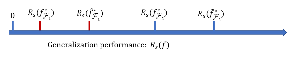
Figure 2: An illustrative example for consistent model comparison when the synthetic and original distributions are not the same.

6.1 Examples for Inconsistent Model Comparison

In this section, we present two illustrative examples for classification and regression to demonstrate that the dissimilarity between the marginal distributions of the synthetic and original features sometimes might lead to distinctive optimal models under the same model specification, which results in inconsistent model comparison. For both examples, we denote the support of synthetic and original features as $\mathcal{X}=[-1,1]$. Let the regression functions in classification and regression be $\eta(x)=1$ for $x\in[0,1]$ and $-1$ otherwise and $\mu(x)=x$. The true feature $X$ and the synthetic feature $\widetilde{X}$ are further assumed to follow the corresponding distributions,

$$\mathbb{P}_{X}(x)=\begin{cases}1-\alpha,&\mbox{ if }x\in[0,1],\\ \alpha,&\mbox{ if }x\in[-1,0).\end{cases}\mbox{ and }\mathbb{P}_{\widetilde{X}}(x)=\begin{cases}\alpha,&\mbox{ if }x\in[0,1],\\ 1-\alpha,&\mbox{ if }x\in[-1,0).\end{cases}$$ (13)

We further assume that the estimation model $\widehat{\mu}$ and $\widehat{\eta}$ are the same as $\mu$ and $\eta$, respectively.

Regression: For the regression task, we suppose there are two model specifications $\mathcal{F}_{1}=\{f(x)=\beta:\beta\in[-1/2,1/2]\}$ and $\mathcal{F}_{2}=\{f(x)=\beta:\beta\in[-1/4,1/4]\}$, the risks under the true and synthetic distributions are, respectively, given as

$$R_{s}(f)=\frac{1}{3}-\beta+\beta^{2}+2\alpha\beta\mbox{ and }\widetilde{R}_{s}(f)=\frac{1}{3}+\beta+\beta^{2}-2\alpha\beta.$$

Let $\alpha=5/6$, we have $R_{s}(f)=\beta^{2}+2\beta/3+1/3$ and $\widetilde{R}_{s}(f)=\beta^{2}-2/3\beta+1/3$. Then we can verify that $f_{\mathcal{F}_{1}}^{*}=-1/3$ and $f_{\mathcal{F}_{2}}^{*}=-1/4$, which leads to $R(f_{\mathcal{F}_{2}}^{*})>R(f_{\mathcal{F}_{1}}^{*})$. Conversely, $\widetilde{f}_{\mathcal{F}_{1}}^{*}=1/3$ and $\widetilde{f}_{\mathcal{F}_{2}}^{*}=1/4$, which leads to $R(\widetilde{f}_{\mathcal{F}_{1}}^{*})>R(\widetilde{f}_{\mathcal{F}_{2}}^{*})$.

Classification: For the classification task, we also suppose there are two model specifications $\mathcal{G}_{1}=\{g(x)=\mathop{\mathrm{sign}}(|x|-\beta):\beta\in[0,1/2]\}$ and $\mathcal{G}_{2}=\{g(x)=\mathop{\mathrm{sign}}(|x|-\beta):\beta\in[1/4,1/3]\}$, the risks of the true and synthetic distributions are, respectively, given as

$$R_{0\text{-1}}(g)=1-\alpha+(2\alpha-1)\beta\mbox{ and }\widetilde{R}_{0\text{-1}}(g)=\alpha-(2\alpha-1)\beta.$$

For any $\alpha>1/2$, we have $g_{\mathcal{G}_{1}}^{*}(x)=\mathop{\mathrm{sign}}(|x|)$ and $g_{\mathcal{G}_{2}}^{*}(x)=\mathop{\mathrm{sign}}(|x|-1/4)$, while $\widetilde{g}_{\mathcal{G}_{1}}^{*}(x)=\mathop{\mathrm{sign}}(|x|-1/2)$ and $\widetilde{g}_{\mathcal{G}_{2}}^{*}(x)=\mathop{\mathrm{sign}}(|x|-1/3)$. Clearly, the model comparison is inconsistent since $R_{0\text{-}1}(\widetilde{g}_{\mathcal{G}_{1}}^{*})<R_{0\text{-}1}(\widetilde{g}_{\mathcal{G}_{2}}^{*})$.

The examples provided illustrate how changes in the marginal distribution of features can influence the optimal model for minimizing risk under a given model specification. While a more flexible model specification can offer better generalization performance by capturing complex relationships between features and the target variable, it also increases the possibility of estimating an inferior model based on synthetic data with low feature fidelity.

6.2 Consistent Model Comparison

In this section, we examine the impact of the quality of synthetic data on the model comparison result. Our goal is to identify sufficient conditions under which the relative performance of estimated models from synthetic data is consistent with that of original data.

To begin with, we present a novel metric called $(V,d)$-fidelity level that evaluates the differences between synthetic and original feature distributions. Our proposed metric resembles $f$-divergences (Rényi,, 1961) in essence, as both rely on density ratios for characterizing distributional difference. The proposed $(V,d)$-fidelity level offers an alternative means of gauging the disparity between two distributions, rather than relying on the $\chi^{2}$-divergence method as presented in Section 4, which could yield infinite values in certain scenarios. In essence, by utilizing the $(V,d)$-fidelity level, we can carry out a more intricate analysis of how the deviation of the synthetic distribution from the original distribution influences downstream model comparison.

Definition 2 ($(V,d)$-fidelity level).

We say the distributions $\mathbb{P}_{\bm{X}}$ and $\mathbb{P}_{\widetilde{\bm{X}}}$ satisfy $(V,d)$-fidelity level if there exist $V\geq 0$ and $0<d\leq\infty$ such that for any $C>0$,

$$\max\left\{\int_{\mathcal{X}_{C}}\mathbb{P}_{\bm{X}}(\bm{x})d\bm{x},\int_{\mathcal{X}_{C}^{\prime}}\mathbb{P}_{\widetilde{\bm{X}}}(\bm{x})d\bm{x}\right\}\leq V\cdot C^{-d},$$ (14)

where $\mathcal{X}_{C}=\left\{\bm{x}\in\mathcal{X}:\mathbb{P}_{\bm{X}}(\bm{x})/\mathbb{P}_{\widetilde{\bm{X}}}(\bm{x})\geq C\right\}$ and $\mathcal{X}_{C}^{\prime}=\left\{\bm{x}\in\mathcal{X}:\mathbb{P}_{\widetilde{\bm{X}}}(\bm{x})/\mathbb{P}_{\bm{X}}(\bm{x})\geq C\right\}$.

It should be noted that the proposed metric in (14) is symmetric and utilizes two parameters $V$ and $d$ to describe the probabilities of areas with high density ratio values. A greater value of $d$ or a smaller value of $V$ signifies a higher degree of similarity between the two distributions.

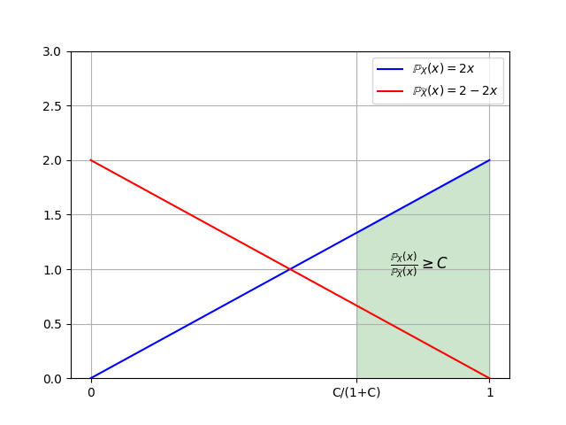
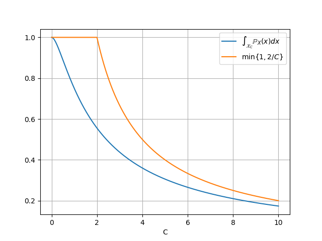
Figure 3: Left: The density functions $\mathbb{P}_{X}(x)=2x$ and $\mathbb{P}_{\widetilde{X}}(x)$ for $x\in[0,1]$, while the shaded area denotes the probability of $\mathcal{X}_{C}$. Right: the values of $\int_{\mathcal{X}_{C}}\mathbb{P}_{X}(x)dx$ for $C\geq 0$ and its decreasing pattern is captured by the upper bound function $2/C$ for large $C$.

Example 1.

Suppose $\mathbb{P}_{X}(x)=2x$ and $\mathbb{P}_{\widetilde{X}}(x)=2-2x$ for $x\in[0,1]$, then $\chi^{2}(\mathbb{P}_{X}\|\mathbb{P}_{\widetilde{X}})=\chi^{2}(\mathbb{P}_{\widetilde{X}}\|\mathbb{P}_{X})=\infty$. However, $\mathbb{P}_{X}$ and $\mathbb{P}_{\widetilde{X}}$ satisfy $(2,1)$-fidelity level.

Example 1 shows that $\chi^{2}$-divergence may fail to capture the difference between two distributions when their density ratio is unbounded which leads to an infinite $\chi^{2}$-divergence. However, as shown in Figure 3, the deviation between the distributions $\mathbb{P}_{X}$ and $\mathbb{P}_{\widetilde{X}}$ is characterized by the proposed metric with $(V,d)=(2,1)$. Additionally, it is possible for a pair of distributions to meet the $(V,d)$-fidelity level for a set of values of $V$ and $d$. For instance, if $\mathbb{P}_{\bm{X}}$ and $\mathbb{P}_{\widetilde{\bm{X}}}$ conform to the $(1,1)$-fidelity level, then they must also meet $(V,d)$-fidelity level for any $V>1$.

Lemma 1.

The following are some examples of $(V,d)$-fidelity level.

• If $\mathbb{P}_{\bm{X}}=\mathbb{P}_{\widetilde{\bm{X}}}$, then $\mathbb{P}_{\bm{X}}$ and $\mathbb{P}_{\widetilde{\bm{X}}}$ satisfy $(1,\infty)$-fidelity level.

• If $M_{1}\leq\mathbb{P}_{\bm{X}}(\bm{x})/\mathbb{P}_{\widetilde{\bm{X}}}(\bm{x})\leq M_{2}$ for some positive constants $M_{1}\in[0,1]$ and $M_{2}\in[1,\infty]$, then $\mathbb{P}_{\bm{X}}$ and $\mathbb{P}_{\widetilde{\bm{X}}}$ satisfy $(\max\{M_{2}^{d},M_{1}^{-d}\},d)$-fidelity level for any $d>0$.

• If $\chi^{2}(\mathbb{P}_{\bm{X}}\|\mathbb{P}_{\widetilde{\bm{X}}})$ and $\chi^{2}(\mathbb{P}_{\widetilde{\bm{X}}}\|\mathbb{P}_{\bm{X}})$ are finite, then $\mathbb{P}_{X}$ and $\mathbb{P}_{\widetilde{X}}$ satisfy $(M_{3},1)$-fidelity level, where $M_{3}=\max\{\chi^{2}(\mathbb{P}_{\bm{X}}\|\mathbb{P}_{\widetilde{\bm{X}}}),\chi^{2}(\mathbb{P}_{\widetilde{\bm{X}}}\|\mathbb{P}_{\bm{X}})\}+1$. Conversely, if $\mathbb{P}_{\bm{X}}$ and $\mathbb{P}_{\widetilde{\bm{X}}}$ satisfy $(V,d)$-fidelity level with $d>1$, then

  $$\max\{\chi^{2}(\mathbb{P}_{\bm{X}}\|\mathbb{P}_{\widetilde{\bm{X}}}),\chi^{2}(\mathbb{P}_{\widetilde{\bm{X}}}\|\mathbb{P}_{\bm{X}})\}\leq(C-1)^{2}+\frac{V\cdot 2^{d}}{C^{d-1}}\cdot(2^{d-1}-1)^{-1},$$

  for any $C\geq 1$.

In Lemma 1, the second example assumes that the ratio of densities is bounded, which is a common assumption in transfer learning (Kpotufe,, 2017) and density ratio estimation (Kato and Teshima,, 2021). The third example establishes the relation between the $\chi^{2}$-divergence used in Section 4 and $(V,d)$-fidelity level, demonstrating that finite $\chi^{2}$-divergences between two distributions are sufficient for them to satisfy the $(V,d)$-fidelity level.

Before we prove the consistent model comparison, we introduce two assumptions.

Assumption 4.

Assume that $\widehat{\eta}$ and $\widehat{\mu}$ are consistent estimators of $\eta$ and $\mu$, respectively, such that $\|\widehat{\eta}-\eta\|_{L^{2}(\mathbb{P}_{\bm{X}})}=o_{p}(1)$ and $\|\widehat{\mu}-\mu\|_{L^{2}(\mathbb{P}_{\bm{X}})}=o_{p}(1)$.

Assumption 4 assumes that the synthetic distributions must accurately capture the relationship between features and response, requiring $\widehat{\eta}$ and $\widehat{\mu}$ converge to $\eta$ and $\mu$, respectively.

Assumption 5.

For two pairs of model classes $(\mathcal{F}_{1},\mathcal{F}_{2})$ and $(\mathcal{G}_{1},\mathcal{G}_{2})$ with $R_{s}(f_{\mathcal{F}_{2}}^{*})<R_{s}(f_{\mathcal{F}_{1}}^{*})$ and $R_{0\text{-}1}(g_{\mathcal{G}_{2}}^{*})<R_{0\text{-}1}(g_{\mathcal{G}_{1}}^{*})$ and $\mathbb{P}_{\bm{X}}$ and $\mathbb{P}_{\widetilde{\bm{X}}}$ satisfying $(V,d)$-fidelity level, we assume that

$$C_{d,V,U}^{2}\big{(}\Phi_{s}(f_{\mathcal{F}_{2}}^{*})\big{)}^{\frac{d^{2}}{(d+1)^{2}}}<\Phi_{s}(f_{\mathcal{F}_{1}}^{*})\mbox{ and }K_{d,V}\big{(}\Phi_{0\text{-}1}(g_{\mathcal{G}_{2}}^{*})\big{)}^{\frac{d^{2}}{(d+1)^{2}}}<\Phi_{0\text{-}1}(g_{\mathcal{G}_{1}}^{*}),$$ (15)

where $C_{d,V,U}=(d^{\frac{1}{d+1}}+d^{-\frac{d}{d+1}})^{\frac{3d+1}{2(d+1)}}V^{\frac{2d+1}{2(d+1)^{2}}}U^{\frac{2d+1}{(d+1)^{2}}}$, $K_{d,V}=(d^{\frac{1}{d+1}}+d^{-\frac{d}{d+1}})^{\frac{2d+1}{d+1}}V^{\frac{2d+1}{(d+1)^{2}}}$, and $U=\sup_{f\in\mathcal{F}_{2}}\|f-\widehat{\mu}\|_{L^{2}(\mathbb{P}_{\bm{X}})}$.

Assumption 5 implicitly imposes a constraint on the difference between the synthetic and original distributions. In other words, the gaps $R_{0\text{-}1}(g_{\mathcal{G}_{1}}^{*})-R_{0\text{-}1}(g_{\mathcal{G}_{2}}^{*})$ and $R_{s}(f_{\mathcal{F}_{1}}^{*})-R_{s}(f_{\mathcal{F}_{2}}^{*})$ should be large enough to counteract the effect yielded by the dissimilarity between the synthetic and original distributions. In particular, when $\mathcal{F}_{2}$ and $\mathcal{G}_{2}$ are chosen appropriately such that $\Phi_{s}(f_{\mathcal{F}_{2}}^{*})=0$ and $\Phi_{0\text{-}1}(g_{\mathcal{G}_{2}}^{*})=0$, Assumption 5 automatically holds true. This case demonstrates that the estimated model under a correct model specification always outperforms other models regardless of the distribution of synthetic features. This result reveals an intriguing phenomenon that the distribution of synthetic features need not be the same as that of the original features for identifying the model class with the best generalization performance based on synthetic data.

Next we present several realizations of Assumption 5 under different relations between $\mathbb{P}_{\bm{X}}$ and $\mathbb{P}_{\widetilde{\bm{X}}}$ for providing a deeper understanding of this assumption.

Example 2.

If $\chi^{2}(\mathbb{P}_{\bm{X}}\|\mathbb{P}_{\widetilde{\bm{X}}})$ and $\chi^{2}(\mathbb{P}_{\widetilde{\bm{X}}}\|\mathbb{P}_{\bm{X}})$ are finite, then the inequalities in (15) become

$$4M_{3}^{3/4}U^{3/4}\Phi_{s}^{1/4}(f_{\mathcal{F}_{2}}^{*})<\Phi_{s}(f_{\mathcal{F}_{1}}^{*})\mbox{ and }2^{3/2}M_{3}^{3/4}\Phi_{0\text{-}1}^{1/4}(g_{\mathcal{G}_{2}}^{*})<\Phi_{0\text{-}1}(g_{\mathcal{G}_{1}}^{*}),$$

where $M_{3}$ is defined in Lemma 1. This example provides an explicit form of Assumption 5 given that the $\chi^{2}$ divergences between the synthetic and original distributions are finite.

Clearly, Assumption 5 is less strict as $\chi^{2}(\mathbb{P}_{\bm{X}}\|\mathbb{P}_{\widetilde{\bm{X}}})$ and $\chi^{2}(\mathbb{P}_{\widetilde{\bm{X}}}\|\mathbb{P}_{\bm{X}})$ are smaller, showing that larger similarity between the synthetic and original distributions of features allows for a smaller gap between the generalization performances of different model classes for consistent model comparison.

Example 3.

If $\Phi_{s}(f_{\mathcal{F}_{2}}^{*})=0$ and $\Phi_{0\text{-}1}(g_{\mathcal{G}_{2}}^{*})=0$, then the inequalities in (15) hold for any synthetic feature distribution $\mathbb{P}_{\widetilde{\bm{X}}}$. This example shows that if one of models for comparison correctly specifies the ground truth model, model comparison based on synthetic data is always consistent regardless of the synthetic distribution of features.

Example 4.

If $\mathbb{P}_{\bm{X}}=\mathbb{P}_{\widetilde{\bm{X}}}$, then the inequalities in (15) become

$$R_{s}(f_{\mathcal{F}_{2}}^{*})<R_{s}(f_{\mathcal{F}_{1}}^{*})\mbox{ and }R_{0\text{-}1}(g_{\mathcal{G}_{2}}^{*})<R_{0\text{-}1}(g_{\mathcal{G}_{1}}^{*}).$$

These two inequalities automatically hold true by presuming that $R_{s}(f_{\mathcal{F}_{2}}^{*})<R_{s}(f_{\mathcal{F}_{1}}^{*})$ and $R_{0\text{-}1}(g_{\mathcal{G}_{2}}^{*})<R_{0\text{-}1}(g_{\mathcal{G}_{1}}^{*})$.

Example 5.

If $M_{1}\leq\mathbb{P}_{\bm{X}}(\bm{x})/\mathbb{P}_{\widetilde{\bm{X}}}(\bm{x})\leq M_{2}$ for some positive constants $M_{1}\in[0,1]$ and $M_{2}\in[1,\infty]$, then the inequalities in (15) become

$$\max\{M_{2}^{2},M_{1}^{-2}\}\cdot\Phi_{s}(f_{\mathcal{F}_{2}}^{*})<\Phi_{s}(f_{\mathcal{F}_{1}}^{*})\mbox{ and }\max\{M_{2}^{2},M_{1}^{-2}\}\cdot\Phi_{0\text{-}1}(g_{\mathcal{G}_{2}}^{*})<\Phi_{0\text{-}1}(g_{\mathcal{G}_{1}}^{*}).$$

This example considers that the density ratio $\mathbb{P}_{\bm{X}}(\bm{x})/\mathbb{P}_{\widetilde{\bm{X}}}(\bm{x})$ is bounded. Then Assumption 5 requires the ratio of excess risks $\Phi_{0\text{-}1}(g_{\mathcal{G}_{1}}^{*})/\Phi_{0\text{-}1}(g_{\mathcal{G}_{2}}^{*})$ and $\Phi_{s}(f_{\mathcal{F}_{1}}^{*})/\Phi_{s}(f_{\mathcal{F}_{2}}^{*})$ to be larger than $\max\{M_{2}^{2},M_{1}^{-2}\}$.

Theorem 4.

Under Assumptions 4 and 5, it holds that

$$\lim_{n\rightarrow\infty}\mathbb{P}\left(R_{s}(\widetilde{f}_{\mathcal{F}_{1}}^{*})>R_{s}(\widetilde{f}_{\mathcal{F}_{2}}^{*})\right)=1\mbox{ and }\lim_{n\rightarrow\infty}\mathbb{P}\left(R_{0\text{-}1}(\widetilde{g}_{\mathcal{G}_{1}}^{*})>R_{0\text{-}1}(\widetilde{g}_{\mathcal{G}_{2}}^{*})\right)=1,$$

where the randomness results from training datasets $\mathcal{D}_{r}$ and $\mathcal{D}_{c}$ used for estimating $\mu$ and $\eta$, respectively.

Theorem 4 shows that consistent model comparison is achieved with a large probability under Assumptions 4 and 5.

7 Numerical Experiments

7.1 Simulation

7.1.1 Consistent Generalization

In this section, we present a series of simulations aimed at validating our theoretical findings. Specifically, the simulations focus on verifying the convergence of the utility metric as described in Equation (5) and investigating how the convergence of these metrics is affected by various factors such as model specification, feature fidelity, and the estimation models used. Our experimental results are in line with our theoretical findings, thereby confirming the tightness and effectiveness of the analytic bounds established in Equations (1) and (2). We consider some practical scenarios in which non-parametric methods are used as the estimation model under different model specifications. The generation of original dataset $\{(\bm{x}_{i},y_{i})\}_{i=1}^{n}$ for regression is structured as follows. First, we generate the original features $\bm{x}i$’s via a truncated multivariate normal distribution (Botev,, 2017) with lower bounds set at $\bm{l}=(-2,-2)$, upper bounds set at $\bm{u}=(2,2)$, and a mean vector of $\bm{m}=(1,1)$. We set $\mu(\bm{x}_{i})=\exp(x_{i1})-\exp(x_{i2})$ and generate true responses $y_{i}$ as $y_{i}=\mu(\bm{x}_{i})+\epsilon_{i}$, where $\epsilon_{i}$ is Gaussian noise with mean $0$ and variance $1$

We consider two non-parametric methods, namely $K$-nearest neighbors (KNN; Coomans and Massart,, 1982) and random forest regressor (RF; Breiman,, 2001; Ho,, 1995), as well as deep neural networks (Farrell et al.,, 2021) for the estimation model. For the hyperparameters, we set the number of neighbors $K$ at the order of $n^{2/(2+p)}$ (Hall et al.,, 2008) in KNN. Additionally, we include the case where $\widehat{\mu}=\mu$ as a baseline. For random forests, we set the numbers of trees and the maximum depth of each tree as $3/2n^{1/2}$ and $\text{log}(n)$, respectively. For the deep neural network, we consider the 4-layer perceptron with hidden units being 10 and ReLU activation function. With the estimation models, we then generate synthetic responses following the procedure illustrated in Figure 1.

We consider the following three specifications of training models: (1) $\mathcal{F}_{1}=\{f(\bm{x})=\beta_{1}x_{1}+\beta_{2}x_{2}:\bm{\beta}\in\mathbb{R}^{2}\}$; (2) $\mathcal{F}_{2}=\{f(\bm{x})=\beta_{1}x_{1}+\beta_{2}x_{2}+\beta_{3}x_{1}^{2}+\beta_{4}x_{2}^{2}:\bm{\beta}\in\mathbb{R}^{4}\}$; (3) $\mathcal{F}_{3}=\{f(\bm{x})=\beta_{1}\exp(x_{1})+\beta_{2}\exp(x_{2}):\bm{\beta}\in\mathbb{R}^{2}\}$. Clearly, $\mathcal{F}_{1}$ is a class of linear models of original features and can be included as a special case by $\mathcal{F}_{2}$. Additionally, $\mathcal{F}_{3}$ refers to as the correct model specification that achieves the optimal generalization error. We generate a testing dataset of 50,000 samples to estimate the risks of the estimated models.

To investigate the effect of feature fidelity on the utility metrics, we consider two scenarios. In Scenario I, the synthetic and original feature distributions are assumed to be the same, and the convergence of utility metrics is analyzed under various model assumptions and estimation methods. In Scenario II, the synthetic feature distribution is a uniform distribution over the same support, and the behavior of utility metrics is studied under three different model specifications. The sample size is set as $n\in\{1000\times 2^{i},i=1,2,3,4,5\}$, and each setting is replicated 100 times to evaluate the convergence of utility metrics. We reports the average estimated utility metrics and their 95% confidence intervals in Figure 4.

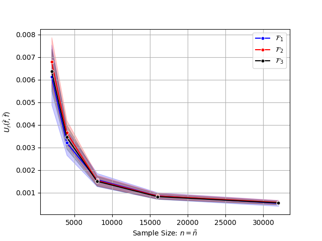
(a) KNN

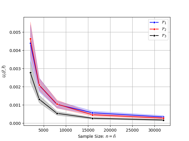
(b) RF

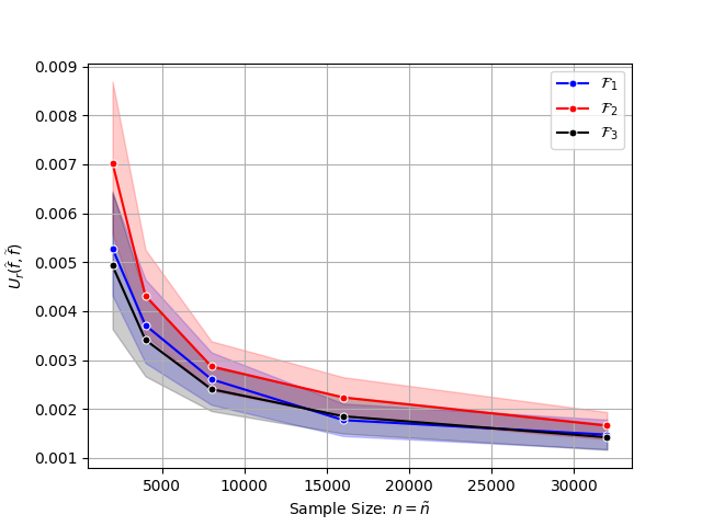
(c) DNN

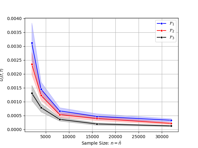
(d) Baseline: $\widehat{\mu}=\mu$

Figure 4: The estimated utility metrics with perfect feature fidelity (Scenario I).

As can be seen in Figure 4, with perfect feature fidelity, the utility metric $U_{r}(\widehat{f},\widetilde{f})$ with different model specifications and estimation methods decrease to zero simultaneously as expected. Compared with other estimation models, the utility metric for $\widehat{\mu}=\mu$ is smaller under different sample sizes, showing that a smaller approximation error of the estimation model increases the similarity between $\widehat{f}$ and $\widetilde{f}$ in generalization for all model specifications.

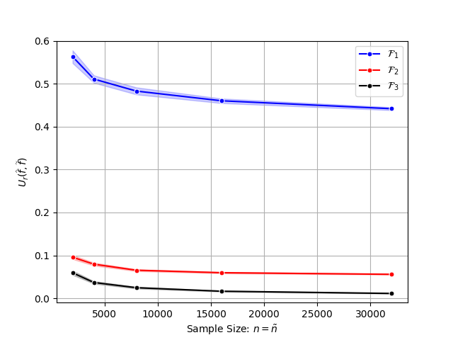
(a) KNN

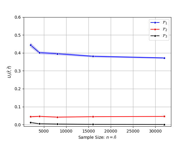
(b) RF

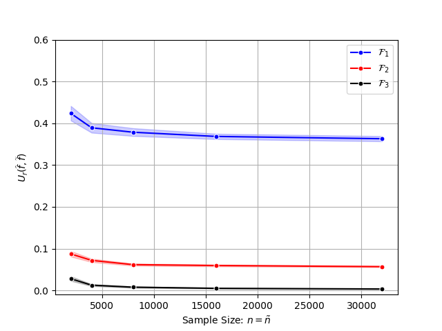
(c) DNN

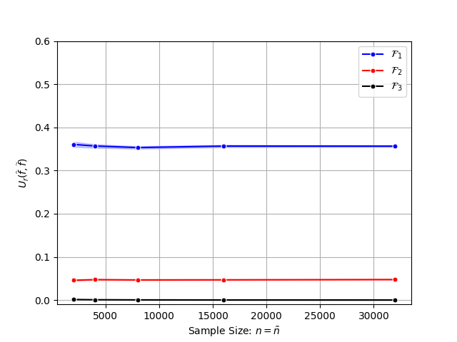
(d) Baseline: $\widehat{\mu}=\mu$

Figure 5: The estimated utility metrics with imperfect feature fidelity (Scenario II).

Figure 5 presents the estimated utility metrics under different model specifications and estimation models given that the distributions of $\bm{X}$ and $\widetilde{\bm{X}}$ are different. In stark contrast, the utility metrics of wrong model specifications $\mathcal{F}_{1}$ and $\mathcal{F}_{2}$ converge to some fixed positive constants as $n$ increases and finally stay unchanged, which is particularly evident when $\widehat{\mu}=\mu$. Conversely, for the correct model specification $\mathcal{F}_{3}$, the utility metrics with different estimation models converge to zero as $n$ increases. These results empirically support our theoretical results.

7.1.2 Consistent Model Comparison

In this section, we conduct an experiment to validate two phenomenon of model comparison based on synthetic data. Specifically, consistency of model comparison based on synthetic data is achievable when one of the models accurately specifies the regression function, or when the generalization gap between two model specifications is wide enough to offset any differences in distribution between synthetic and real features.

We generate real data as follows. First, we generate real features as $x_{i}\sim\text{Unif}(0,2)$ for $i=1,\ldots,n$. Then we consider the regression function $y_{i}=\bm{u}_{i}^{T}\bm{\beta}$, where $\bm{u}_{i}=((x_{i}+0.1)^{-1},x_{i},x_{i}^{2},x_{i}^{3})$ and $\bm{\beta}=(1,-2,-2,1)$. For the downstream learning tasks, we consider the following four specifications of training models: (1) $\mathcal{F}_{0}=\{f(x)=\beta_{1}x+\beta_{2}x^{3}:\bm{\beta}\in\mathbb{R}^{2}\}$; (2) $\mathcal{F}_{1}=\{f(\bm{x})=\beta_{1}(x+0.1)^{-1}+\beta_{2}x^{3}:\bm{\beta}\in\mathbb{R}^{2}\}$; (3) $\mathcal{F}_{2}=\{f(\bm{x})=\beta_{1}x^{2}+\beta_{2}x^{3}:\bm{\beta}\in\mathbb{R}^{2}\}$; (4) $\mathcal{F}_{3}=\{f(\bm{x})=\beta_{1}(x+0.1)^{-1}+\beta_{2}x+\beta_{3}x^{2}+\beta_{4}x^{3}:\bm{\beta}\in\mathbb{R}^{4}\}$. Here $\mathcal{F}_{3}$ is considered the correct model specification. To generate synthetic features $\widetilde{x}_{i}$, we use the density function $\mathbb{P}_{\widetilde{X}}(x)=\alpha(x-1)+1$ for $x\in[0,2]$, where $a\in[0,1/2]$ is a parameter that controls the distribution similarity between $X$ and $\widetilde{X}$. As $\alpha$ increases, the distribution of $\widetilde{X}$ becomes less similar to that of $X$. The case where $\alpha=0$ corresponds to $X=\widetilde{X}$. It’s important to note that we assume the estimation model is perfect, meaning that $\widetilde{y}_{i}=\widetilde{\bm{u}}_{i}^{T}\bm{\beta}$, where $\widetilde{\bm{u}}_{i}=((\widetilde{x}_{i}+0.1)^{-1},\widetilde{x}_{i},\widetilde{x}_{i}^{2},\widetilde{x}_{i}^{3})$. For each setting, we generate 10,000 real samples and 10,000 synthetic samples for training and evaluate the fitted models on 50,000 real samples. The generalization performances of fitted models from real and synthetic data over 100 replications are reported in Figure 6.

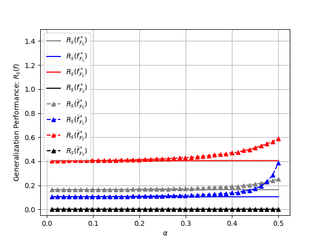
Figure 6: The generalization performances of models estimated from synthetic data and original data under different model specifications.

Figure 6 demonstrates that the black dashed curve consistently lies below the other dashed curves for various values of $\alpha$, indicating that consistent model comparison is achieved when one of the models for comparison is accurate. This result is aligns with Theorem 4 since Assumption 5 holds true in this scenario. Additionally, as the synthetic feature distribution becomes less similar to the real feature distribution, the generalization performances of models trained on synthetic data worsen. Among the blue, red, and grey dashed curves, the blue curve appears to be the most affected by changes in the synthetic feature distribution, and eventually leads to inconsistent model comparison between $\mathcal{F}_{1}$ and $\mathcal{F}_{0}$, where $R_{s}(\widetilde{f}_{\mathcal{F}_{1}}^{*})$ becomes greater than $R_{s}(\widetilde{f}_{\mathcal{F}_{0}}^{*})$. Nevertheless, $R_{s}(\widetilde{f}_{\mathcal{F}_{1}}^{*})$ remains below $R_{s}(\widetilde{f}_{\mathcal{F}_{2}}^{*})$ due to the wide gap between $R_{s}(f_{\mathcal{F}_{1}}^{*})$ and $R_{s}(f_{\mathcal{F}_{2}}^{*})$. This finding confirms our theoretical results in Section 6 that consistent model comparison based on synthetic data requires a substantial generalization gap between two model specifications to offset the impact of any differences between distributions of synthetic and actual features.

7.2 Real Experiment: MNIST Dataset

In this section, we use the MNIST dataset (LeCun,, 1998) as an example to demonstrate how models trained on synthetic data can generalize well on real data with appropriate model specification, even when the quality of the synthetic data is subpar. The MNIST dataset comprises 60,000 training images and 10,000 testing images, with each sample being a 28$\times$28 grey-scale pixel image of one of the 10 digits. We utilize a GAN (Goodfellow et al.,, 2020) to generate synthetic images. The generator and discriminator both have three-layer perceptrons with a LeakyReLu activation function. The generator takes 100-dimensional Gaussian noise as input and outputs 784-dimensional vectors, which are then reshaped into 28$\times$28 images. We employ Adam as the optimizer with a learning rate of 0.001 and use generators trained for 100 and 400 epochs to generate two sets of synthetic images representing different feature fidelity levels. As depicted in Figure 7, as the training epoch increases, synthetic images become clearer and more closely resemble true images. Additionally, the two synthetic image datasets have the same size as the original dataset for each digit.

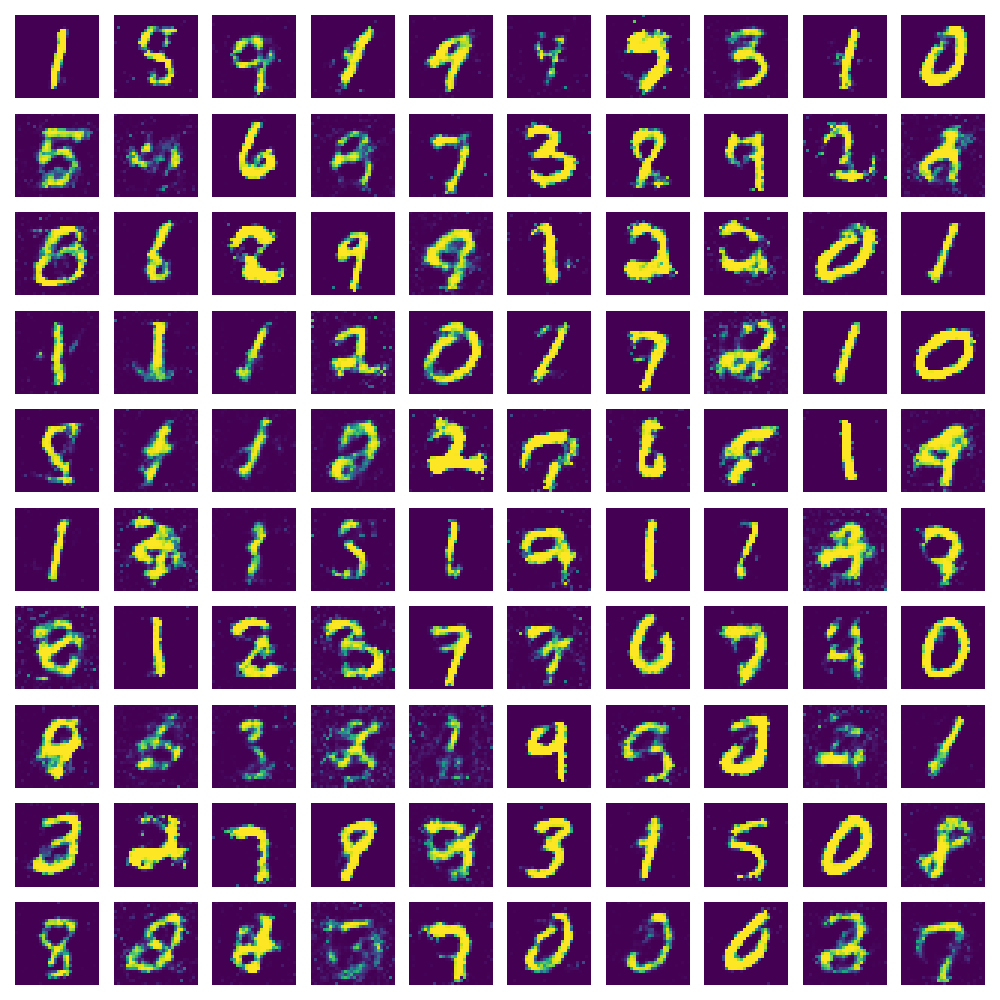
(a) 100 epochs

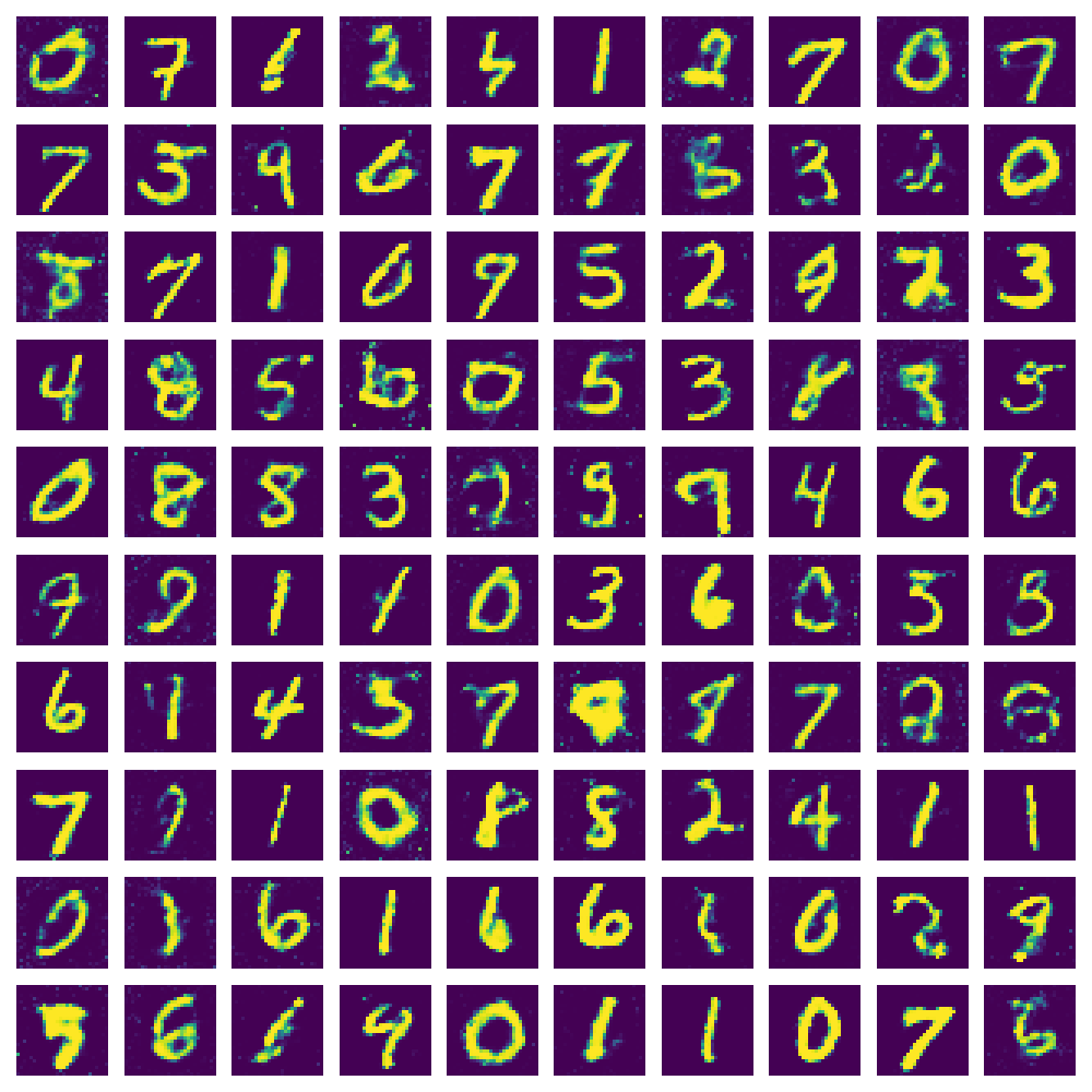
(b) 400 epochs

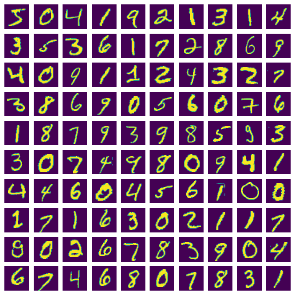
(c) Raw images

Figure 7: Synthetic images generated by GANs at different epochs and real images

In this experiment, we utilize a neural network consisting of two convolution layers with ReLU activation and two fully-connected layers to generate responses for synthetic images. The kernel sizes and the number of channels for the convolution layers are set as $4\times 4$ and 28, respectively, and each convolution layer is followed by a max pooling layer with size $2\times 2$. The first fully-connected layer comprises 128 hidden units with ReLU activation, while the last layer utilizes softmax activation to output the probability for each class. The neural network is trained using the Adam optimizer with a learning rate of 0.001 for 10 epochs, achieving nearly 99% accuracy on testing samples. Thus, this convolutional neural network accurately approximates the relationship between real images and their corresponding responses.

To highlight the significance of model specification, we have considered three distinct model specifications: (1) a single-layer perceptron that takes flattened images as input and produces the probability of each class as output; (2) a two-layer perceptron with 128 hidden units; and (3) a model that is identical to the one employed to generate synthetic responses. To keep a check on the training loss, the early-stopping technique is employed. The accuracies on testing samples have been reported in Figure 8, which have been averaged over 30 replications.

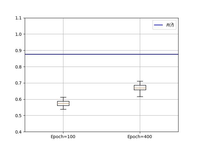
(a) Model 1

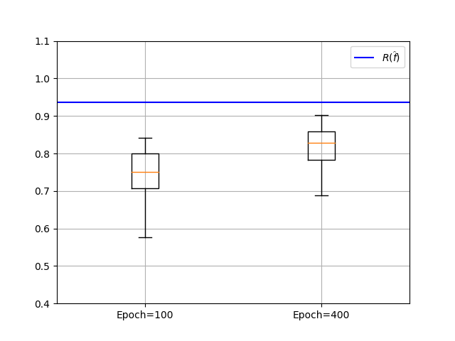
(b) Model 2

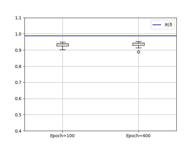
(c) Model 3

Figure 8: The testing accuracies on 10,000 real images of different model specifications and two generators trained in 100 and 400 epochs, respectively. The blue line denotes the testing accuracy of the model trained on the raw training dataset under the same model specification.

Figure 8 depicts the impact of increasing training epochs on the performance of all three model specifications, which demonstrates that higher quality synthetic images lead to improved model performance. Notably, Model 1 and Model 2 exhibit a significant drop in generalization accuracy on testing samples when the real dataset is substituted with synthetic data, achieving only 61.4% and 71.8%, respectively, compared to the accuracies of 87.5% and 93.6% achieved when trained on real data. Conversely, the drop in generalization accuracy is less severe for Model 3, which aligns with our theoretical findings that an accurate model specification is more important than the feature fidelity of synthetic data in yielding comparable performance to real data.

This Appendix provides detailed proofs for all theorems and lemma in the manuscript. For theoretical proofs in the following, we introduce the concept of $\epsilon$-covering set. If $\mathcal{C}$ is a $\epsilon$-covering set of a function class $\mathcal{F}$ with metric $\|\cdot\|_{L^{2}(\mathbb{P}_{\bm{X}})}$, then for any $f\in\mathcal{F}$, there exists $f^{\prime}\in\mathcal{C}$ such that $\|f^{\prime}-f\|_{L^{2}(\mathbb{P}_{\bm{X}})}<\epsilon$.

S.1 Auxiliary Results

S.1.1 An Example of Utility Metric for Classification

In this section, we offer an illustrative example of classification as a supplement to Section 5. The purpose is to demonstrate that the utility metric of classification does not converge when there is imperfect feature fidelity and an incorrect model specification. The example we consider is one-dimensional linear classification. We assume $\mathcal{X}=[-1,1]$ and define the classification function $\eta(x)$ such that $\eta(x)=1$ for any $x\in(0,1]$ and $\eta(x)=-1$ otherwise. Let $X$ and $\widetilde{X}$ follow the distributions as

$$\mathbb{P}_{X}(x)=\begin{cases}1-\alpha,&\mbox{ if }x\in[0,1],\\ \alpha,&\mbox{ if }x\in[-1,0).\end{cases}\mbox{ and }\mathbb{P}_{\widetilde{X}}(x)=\begin{cases}\alpha,&\mbox{ if }x\in[0,1],\\ 1-\alpha,&\mbox{ if }x\in[-1,0).\end{cases}$$

Incorrect Model Specification: In the downstream classification task, we suppose that the class of classifiers $\mathcal{G}=\{g(x)=\mathop{\mathrm{sign}}(\beta|x|):\beta\in\{-1,1\}\}$ is considered. The risks of any $g\in\mathcal{G}$ under the true and synthetic distributions can be written as

$$R_{0\text{-}1}(g)=(1-\alpha)I\left(\beta\leq 0\right)+\alpha I\left(\beta\geq 0\right)\mbox{ and }\widetilde{R}_{0\text{-}1}(g)=(1-\alpha)I\left(\beta\geq 0\right)+\alpha I\left(\beta\leq 0\right).$$

Suppose there are infinite samples in the real and synthetic datasets, then we have

$$\widehat{g}(x)=\begin{cases}\mathop{\mathrm{sign}}(-x),&\mbox{ if }\alpha>1/2,\\ \mathop{\mathrm{sign}}(x),&\mbox{ if }\alpha<1/2.\end{cases}\mbox{ and }\widetilde{g}(x)=\begin{cases}\mathop{\mathrm{sign}}(x),&\mbox{ if }\alpha>1/2,\\ \mathop{\mathrm{sign}}(-x),&\mbox{ if }\alpha<1/2.\end{cases}$$

Therefore, we obtain

$$U_{c}(\widehat{g},\widetilde{g})=\big{|}R_{0\text{-}1}(\widehat{g})-R_{0\text{-}1}(\widetilde{g})\big{|}=|2\alpha-1|>0,$$ (S1)

for any $\alpha\in(0,1/2)\cup(1/2,1)$. As can be seen in (S1), the utility metric $U_{c}(\widehat{g},\widetilde{g})$ for classification can be bounded away from 0 given inaccurate model specification and imperfect feature fidelity.

Correct Model Specification: If $\mathcal{G}$ includes the Bayes classifier, say $\mathcal{G}=\{g(x)=\mathop{\mathrm{sign}}(\beta x):\beta\in\{-1,1\}\}$. The risks of any $g\in\mathcal{G}$ are given as

$$R_{0\text{-}1}(g)=I(\beta\leq 0)\mbox{ and }\widetilde{R}_{0\text{-}1}(g)=I(\beta\leq 0).$$

This result shows that even though the distribution of $\widetilde{X}$ is not identical to that of $X$, $U_{c}(\widehat{g},\widetilde{g})\equiv 0$ for any $\alpha$ in $\mathbb{P}_{\widetilde{X}}$. This example also validates the second conclusion for classification as stated in Section 4.

S.1.2 Example: Logistic Regression

This section aims to demonstrate our theoretical results for classification using logistic regression, as discussed in Section 5.2. We consider a scenario where $\mathbb{P}_{\widetilde{\bm{X}}}$ is fixed and independent of $\{\bm{x}_{i}\}_{i=1}^{n}$. We denote the original and synthetic datasets in the logistic regression as $\mathcal{D}_{c}=\{(\bm{x}_{i},z_{i})\}_{i=1}^{n}$ and $\widetilde{\mathcal{D}}_{c}=\{(\widetilde{\bm{x}}_{i},\widetilde{z}_{i})\}_{i=1}^{\widetilde{n}}$, respectively. For any given feature $\bm{x}_{i}$, we suppose its associated response $z_{i}$ is generated as follows:

$$z_{i}=\begin{cases}1,&\mbox{ with probability }\eta(\bm{x}_{i}),\\ -1,&\mbox{ with probability }1-\eta(\bm{x}_{i}),\end{cases}$$

where $\eta(\bm{x}_{i})=1/\big{(}1+\exp(-\bm{x}_{i}^{T}\bm{\beta}^{*})\big{)}$.

To generate synthetic responses $\widetilde{z}_{i}$’s, we assume that the maximum likelihood estimator (MLE) is employed to generate synthetic responses and given as follow

$$\widehat{\bm{\beta}}=\mathop{\mathrm{argmin}}_{\bm{\beta}\in\mathbb{R}^{p}}\frac{1}{n}\sum_{i=1}^{n}\log\Big{(}1+\exp(-z_{i}\bm{x}_{i}^{T}\bm{\beta})\Big{)}.$$

With $\widehat{\bm{\beta}}$, for any given synthetic feature $\widetilde{\bm{x}}_{i}$, the synthetic response $\widetilde{z}_{i}$ is generated via the following distribution.

$$\widetilde{z}_{i}=\begin{cases}1,&\mbox{ with probability }\widehat{\eta}(\widetilde{\bm{x}}_{i}),\\ -1,&\mbox{ with probability }1-\widehat{\eta}(\widetilde{\bm{x}}_{i}),\end{cases}$$

where $\widehat{\eta}(\bm{x}_{i})=1/\big{(}1+\exp(-\bm{x}_{i}^{T}\widehat{\bm{\beta}})\big{)}$.

In the downstream classification task, we suppose the model specification is correct with $\mathcal{G}=\{g(\bm{x})=\bm{x}^{T}\bm{\beta}:\bm{\beta}\in[-B,B]^{p}\}$, where $B$ is a constant chosen to satisfy $\|\bm{\beta}^{*}\|_{\infty}<B/2$. Then the estimated models based on $\mathcal{D}_{c}$ and $\widetilde{\mathcal{D}}_{c}$, respectively, are given as

$$\widehat{g}_{log}=\mathop{\mathrm{argmin}}_{g\in\mathcal{G}}\frac{1}{n}\sum_{i=1}^{n}\log\Big{(}1+\exp(-z_{i}g(\bm{x}_{i}))\Big{)},$$

$$\widetilde{g}_{log}=\mathop{\mathrm{argmin}}_{g\in\mathcal{G}}\frac{1}{n}\sum_{i=1}^{n}\log\Big{(}1+\exp(-\widetilde{z}_{i}g(\widetilde{\bm{x}}_{i}))\Big{)}.$$

It is straightforward to verify that $1/(1+\exp(-\widehat{g}_{log}))$ is identical to the estimation model $\widehat{\eta}$ used to generate synthetic responses if $\|\widehat{\bm{\beta}}\|_{\infty}\leq B$.

Theorem S5.

Suppose that $\mathcal{X}$ is a compact set and there exists a positive constant $C_{1}$ such that $\mathbb{P}_{\widetilde{\bm{X}}}(\bm{x})/\mathbb{P}_{\bm{X}}(\bm{x})\leq C_{1}$ for any $\bm{x}\in\mathcal{X}$. Then, for any $\delta>0$,

$$\lim_{n\rightarrow\infty}\lim_{\widetilde{n}\rightarrow\infty}\mathbb{P}\left(U_{c}(\widetilde{g}_{log},\widehat{g}_{log})>\delta\right)=0.$$

In Theorem S5, we present a result regarding the convergence of the utility metric in logistic regression, but we do not provide the explicit forms of the analytic bound because the analytic solution of logistic regression is not obtainable. Theorem S5 shows that the utility metric $U_{c}(\widetilde{g}_{log},\widehat{g}_{log})$ approaches 0 with a high probability, and this convergence becomes more certain as both $n$ and $\widetilde{n}$ increase to infinity. Importantly, this result does not require the distributions of $\bm{X}$ and $\widetilde{\bm{X}}$ to be the same, which is consistent with the second conclusion in Section 4.

S.1.3 Correct Model Specification: Linear Regression and Logistic Regression

This part mainly studies the convergence of utility metrics for linear regression and logistic regression under imperfect feature fidelity (i.e., $\chi^{2}(\mathbb{P}_{\bm{X}}\|\mathbb{P}_{\widetilde{\bm{X}}})\neq 0$). For both tasks, we generate true features $\bm{x}_{i}$’s via a truncated multivariate normal distribution with mean 0 (Botev,, 2017), that is $\bm{x}_{i}\sim\text{TN}(\bm{0},\bm{I},\bm{l},\bm{u})$, where $\bm{0}$ is the mean vector, $\bm{I}$ is the identity covariance matrix, $\bm{l}$ and $\bm{u}$ are both $d$-dimensional vectors representing the lower bounds and upper bounds for all dimensions, respectively. As for synthetic features, we generate $\{\widetilde{\bm{x}}_{i}\}_{i=1}^{\widetilde{n}}$ via a uniform distribution with the same support $\widetilde{\bm{x}}_{i}\sim\text{Unif}(\bm{l},\bm{u})$. To generating synthetic responses in linear regression and logistic regression, we follow the settings in Section 5. Additionally, we generate 50,000 testing samples from the true distributions for estimating the risks in both regression and classification.

(a) Linear Regression

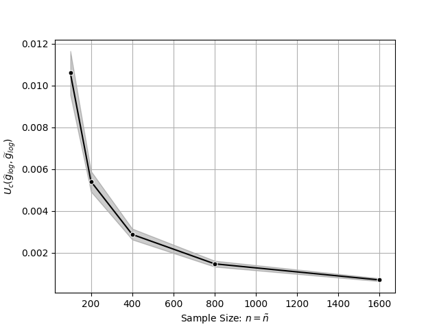
(b) Logistic Regression

Figure 9: The estimated utility metrics in linear regression (Left) and logistic regression (Right) of different sample sizes.

We consider cases $n\in\{100\times 2^{i}:i=1,2,3,4\}$ in both the linear regression and the logistic regression, with $\bm{l}=(-4,-4,-4,-4)$ and $\bm{u}=(4,4,4,4)$, respectively. The averaged estimated utility metrics and their 95% confidence intervals are shown in Figure 9 after 500 replications of each scenario. The estimated utility metrics clearly converge to 0 as sample size $n$ grows, despite the fact that synthetic features and original features have distinct distributions. This indicates that correct model specification allows for the creation of synthetic datasets with high utility but poor feature fidelity.

S.2 Proof of Main Theorems

S.2.1 Proof of Theorem 1

By the triangle inequality, $U_{r}(\widetilde{f},\widehat{f})$ can be upper bounded as

$$U_{r}(\widetilde{f},\widehat{f})\leq\big{|}R_{s}\big{(}\widetilde{f}\big{)}-R_{s}\big{(}f^{*}_{\mathcal{F}}\big{)}\big{|}+\big{|}R_{s}\big{(}\widehat{f}\big{)}-R_{s}\big{(}f_{\mathcal{F}}^{*}\big{)}\big{|},$$ (S2)

where $f^{*}_{\mathcal{F}}=\mathop{\mathrm{argmin}}_{f\in\mathcal{F}}R_{s}(f)$ denotes the optimal function in $\mathcal{F}$ for approximating $\mu$. Here $R_{s}\big{(}\widehat{f}\big{)}-R_{s}\big{(}f_{\mathcal{F}}^{*}\big{)}$ basically measures the estimation error in statistical learning theory and is always positive due to the optimality of $f^{*}_{\mathcal{F}}$.

Next, we proceed to bound the term $\big{|}R_{s}\big{(}\widetilde{f}\big{)}-R_{s}\big{(}f^{*}_{\mathcal{F}}\big{)}\big{|}$. By the fact that $R_{s}(f)=\Phi_{s}(f)+\sigma^{2}$ for any $f\in\mathcal{F}$, we have

$$\big{|}R_{s}\big{(}\widetilde{f}\big{)}-R_{s}\big{(}f^{*}_{\mathcal{F}}\big{)}\big{|}=\big{|}\Phi_{s}\big{(}\widetilde{f}\big{)}-\Phi_{s}\big{(}f^{*}_{\mathcal{F}}\big{)}\big{|}$$

$$\leq \big{|}\Phi_{s}\big{(}\widetilde{f}\big{)}-\widetilde{\Phi}_{s}\big{(}\widetilde{f}\big{)}\big{|}+\big{|}\widetilde{\Phi}_{s}\big{(}\widetilde{f}\big{)}-\widetilde{\Phi}_{s}\big{(}\widetilde{f}_{\mathcal{F}}^{*}\big{)}\big{|}+\big{|}\widetilde{\Phi}_{s}\big{(}\widetilde{f}_{\mathcal{F}}^{*}\big{)}-\Phi_{s}\big{(}\widetilde{f}_{\mathcal{F}}^{*}\big{)}\big{|}+\big{|}\Phi_{s}\big{(}\widetilde{f}_{\mathcal{F}}^{*}\big{)}-\Phi_{s}\big{(}f^{*}_{\mathcal{F}}\big{)}\big{|},$$

where $\widetilde{\Phi}_{s}(f)=\int_{\mathcal{X}}\big{(}f(\bm{x})-\widehat{\mu}(\bm{x})\big{)}^{2}\mathbb{P}_{\widetilde{\bm{X}}}(\bm{x})d\bm{x}$ and $\widetilde{f}_{\mathcal{F}}^{*}=\mathop{\mathrm{argmin}}_{f\in\mathcal{F}}\mathbb{E}_{\bm{\widetilde{X}},\widetilde{Y}}\big{[}(f(\bm{\widetilde{X}})-\widetilde{Y})^{2}\big{]}$.

Notice that $\big{|}\widetilde{\Phi}_{s}(\widetilde{f})-\widetilde{\Phi}_{s}(\widetilde{f}_{\mathcal{F}}^{*})\big{|}$ also measures the estimation error of $\widetilde{f}$ under the synthetic distribution, it remains to bound $|\Phi_{s}\big{(}f\big{)}-\widetilde{\Phi}_{s}\big{(}f\big{)}|$ and $\big{|}\Phi_{s}\big{(}\widetilde{f}_{\mathcal{F}}^{*}\big{)}-\Phi_{s}\big{(}f^{*}_{\mathcal{F}}\big{)}\big{|}$, separately. We first bound $\big{|}\Phi_{s}\big{(}f\big{)}-\widetilde{\Phi}_{s}\big{(}f\big{)}\big{|}$ for cases $f=\widetilde{f}$ and $f=\widetilde{f}_{\mathcal{F}}^{*}$. By the definitions of $\Phi_{s}$ and $\widetilde{\Phi}_{s}$, we have

$$\big{|}\Phi_{s}\big{(}f\big{)}-\widetilde{\Phi}_{s}\big{(}f\big{)}\big{|}= \Big{|}\int_{\mathcal{X}}\big{(}f(\bm{x})-\mu(\bm{x})\big{)}^{2}\mathbb{P}_{\bm{X}}\big{(}\bm{x}\big{)}d\bm{x}-\int_{\mathcal{X}}\big{(}f(\bm{x})-\widehat{\mu}(\bm{x})\big{)}^{2}\mathbb{P}_{\widetilde{\bm{X}}}\big{(}\bm{x}\big{)}d\bm{x}\Big{|}$$

$$\leq \Big{|}\mathbb{E}_{\bm{X}}\left[\big{(}f(\bm{X})-\mu(\bm{X})\big{)}^{2}\right]-\mathbb{E}_{\bm{X}}\left[\big{(}f(\bm{X})-\widehat{\mu}(\bm{X})\big{)}^{2}\right]\Big{|}$$

$$+\left|\mathbb{E}_{\bm{X}}\left[\big{(}f(\bm{X})-\widehat{\mu}(\bm{X})\big{)}^{2}\right]-\mathbb{E}_{\widetilde{\bm{X}}}\left[\big{(}f(\bm{X})-\widehat{\mu}(\bm{X})\big{)}^{2}\right]\right|\triangleq I_{1}+I_{2}.$$

Next, we proceed to bound $I_{1}$ and $I_{2}$ separately. For $I_{2}$, we have

$$I_{2}= \Big{|}\mathbb{E}_{\bm{X}}\left[\big{(}f(\bm{X})-\widehat{\mu}(\bm{X})\big{)}^{2}\right]-\mathbb{E}_{\widetilde{\bm{X}}}\left[\big{(}f(\bm{X})-\widehat{\mu}(\bm{X})\big{)}^{2}\right]\Big{|}$$

$$\leq \int_{\mathcal{X}}\big{(}f(\bm{x})-\widehat{\mu}(\bm{x})\big{)}^{2}\Big{|}\mathbb{P}_{\widetilde{\bm{X}}}(\bm{x})-\mathbb{P}_{\bm{X}}(\bm{x})\Big{|}d\bm{x}$$

$$= \int_{\mathcal{X}}\big{(}f(\bm{x})-\widehat{\mu}(\bm{x})\big{)}^{2}\mathbb{P}_{\widetilde{\bm{X}}}(\bm{x})\Big{|}\frac{\mathbb{P}_{\bm{X}}(\bm{x})}{\mathbb{P}_{\widetilde{\bm{X}}}(\bm{x})}-1\Big{|}d\bm{x}$$

$$\leq 2M\sqrt{\int_{\mathcal{X}}\big{(}f(\bm{x})-\widehat{\mu}(\bm{x})\big{)}^{2}\mathbb{P}_{\widetilde{\bm{X}}}(\bm{x})d\bm{x}}\cdot\sqrt{\int_{\mathcal{X}}\mathbb{P}_{\widetilde{\bm{X}}}(\bm{x})\Big{(}1-\frac{\mathbb{P}_{\bm{X}}(\bm{x})}{\mathbb{P}_{\widetilde{\bm{X}}}(\bm{x})}\Big{)}^{2}d\bm{x}}$$

$$= 2M\sqrt{\widetilde{\Phi}_{s}(f)}\cdot\sqrt{\chi^{2}\big{(}\mathbb{P}_{\bm{X}}\|\mathbb{P}_{\widetilde{\bm{X}}}\big{)}}=C_{1}(f)\sqrt{\chi^{2}\big{(}\mathbb{P}_{\bm{X}}\|\mathbb{P}_{\widetilde{\bm{X}}}\big{)}},$$

where $C_{1}(f)=2M\sqrt{\widetilde{\Phi}_{s}(f)}$, $\chi^{2}\big{(}\mathbb{P}_{\widetilde{\bm{X}}}\|\mathbb{P}_{\bm{X}}\big{)}$ is the $\chi^{2}$-divergence between the distributions of $\widetilde{\bm{X}}$ and $\bm{X}$, and the last inequality follows from the Cauchy-Schwarz inequality, and the second inequality follows by requiring $\max\{\|\widehat{\mu}\|_{L^{\infty}(\mathbb{P}_{\bm{X}})},\|\widetilde{f}\|_{L^{\infty}(\mathbb{P}_{\bm{X}})},\|\widetilde{f}_{\mathcal{F}}^{*}\|_{L^{\infty}(\mathbb{P}_{\bm{X}})},\|f_{\mathcal{F}}^{*}\|_{L^{\infty}(\mathbb{P}_{\bm{X}})}\}\leq M$.

For $I_{1}$, it follows from Cauchy-Schwarz inequality that

$$I_{1}= \Big{|}\int_{\mathcal{X}}\big{(}f(\bm{x})-\widehat{\mu}(\bm{x})\big{)}^{2}\mathbb{P}_{\bm{X}}(\bm{x})d\bm{x}-\int_{\mathcal{X}}\big{(}f(\bm{x})-\mu(\bm{x})\big{)}^{2}\mathbb{P}_{\bm{X}}(\bm{x})d\bm{x}\Big{|}$$

$$\leq \mathbb{E}_{\bm{X}}\Big{[}\Big{(}2f(\bm{X})-\widehat{\mu}(\bm{X})-\mu(\bm{X})\Big{)}\Big{(}\widehat{\mu}(\bm{X})-\mu(\bm{X})\Big{)}\Big{]}$$

$$\leq \sqrt{\mathbb{E}_{\bm{X}}\Big{[}\Big{(}2f(\bm{X})-\widehat{\mu}(\bm{X})-\mu(\bm{X})\Big{)}^{2}\Big{]}}\cdot\sqrt{\mathbb{E}_{\bm{X}}\Big{[}\Big{(}\widehat{\mu}(\bm{X})-\mu(\bm{X})\Big{)}^{2}\Big{]}}$$

$$= \|2f-\widehat{\mu}-\mu\|_{L_{2}(\mathbb{P}_{\bm{X}})}\cdot\sqrt{\Phi_{s}(\widehat{\mu})}\leq 2\sqrt{\Phi_{s}(f)}\sqrt{\Phi_{s}(\widehat{\mu})}+\Phi_{s}(\widehat{\mu}).$$

Combining the upper bounds of $I_{1}$ and $I_{2}$ yields that

$$\big{|}\Phi_{s}\big{(}f\big{)}-\widetilde{\Phi}_{s}\big{(}f\big{)}\big{|}\leq 2M\sqrt{\widetilde{\Phi}_{s}(f)}\cdot\sqrt{\chi^{2}\big{(}\mathbb{P}_{\bm{X}}\|\mathbb{P}_{\widetilde{\bm{X}}}\big{)}}+2\sqrt{\Phi_{s}(f)}\sqrt{\Phi_{s}(\widehat{\mu})}+\Phi_{s}(\widehat{\mu}).$$

Next, we proceed to bound $\big{|}\Phi_{s}(\widetilde{f}_{\mathcal{F}}^{*})-\Phi_{s}(f^{*}_{\mathcal{F}})\big{|}$. By the optimality of $\widetilde{f}_{\mathcal{F}}^{*}$ and $f^{*}_{\mathcal{F}}$, we have

$$\Phi_{s}(\widetilde{f}_{\mathcal{F}}^{*})-\Phi_{s}(f^{*}_{\mathcal{F}})\geq 0\mbox{ and }\widetilde{\Phi}_{s}(f_{\mathcal{F}}^{*})-\widetilde{\Phi}_{s}(\widetilde{f}_{\mathcal{F}}^{*})\geq 0.$$

It then follows that

$$\Phi_{s}(\widetilde{f}_{\mathcal{F}}^{*})-\Phi_{s}(f^{*}_{\mathcal{F}}) \leq\big{(}\Phi_{s}(\widetilde{f}_{\mathcal{F}}^{*})-\widetilde{\Phi}_{s}(\widetilde{f}_{\mathcal{F}}^{*})\big{)}-\big{(}\Phi_{s}(f^{*}_{\mathcal{F}})-\widetilde{\Phi}_{s}(f^{*}_{\mathcal{F}})\big{)}$$

$$\leq\big{|}\Phi_{s}(\widetilde{f}_{\mathcal{F}}^{*})-\widetilde{\Phi}_{s}(\widetilde{f}_{\mathcal{F}}^{*})\big{|}+\big{|}\Phi_{s}(f^{*}_{\mathcal{F}})-\widetilde{\Phi}_{s}(f^{*}_{\mathcal{F}})\big{|}.$$

Therefore, by the fact that $\big{|}\widetilde{\Phi}_{s}(\widetilde{f})-\widetilde{\Phi}_{s}(\widetilde{f}_{\mathcal{F}}^{*})\big{|}=\big{|}\widetilde{R}_{s}(\widetilde{f})-\widetilde{R}_{s}(\widetilde{f}_{\mathcal{F}}^{*})\big{|}$ and $\big{|}\Phi_{s}(\widehat{f})-\Phi_{s}(f^{*}_{\mathcal{F}})\big{|}=\big{|}R_{s}(\widehat{f})-R_{s}(f^{*}_{\mathcal{F}})\big{|}$, we have

$$U_{r}(\widetilde{f},\widehat{f})\leq\big{|}\widetilde{R}_{s}(\widetilde{f})-\widetilde{R}_{s}(\widetilde{f}_{\mathcal{F}}^{*})\big{|}+\big{|}R_{s}(\widehat{f})-R_{s}(f^{*}_{\mathcal{F}})\big{|}$$

$$+2M\Big{(}\sqrt{\widetilde{\Phi}_{s}(\widetilde{f})}+2\sqrt{\widetilde{\Phi}_{s}(\widetilde{f}_{\mathcal{F}}^{*})}+\sqrt{\widetilde{\Phi}_{s}(f^{*}_{\mathcal{F}})}\Big{)}\sqrt{\chi^{2}\big{(}\mathbb{P}_{\bm{X}}\|\mathbb{P}_{\widetilde{\bm{X}}}\big{)}}$$

$$+2\Big{(}\sqrt{\Phi_{s}(\widetilde{f})}+2\sqrt{\Phi_{s}(\widetilde{f}_{\mathcal{F}}^{*})}+\sqrt{\Phi_{s}(f^{*}_{\mathcal{F}})}\Big{)}\sqrt{\Phi_{s}(\widehat{\mu})}$$

$$+4\Phi_{s}(\widehat{\mu}).$$

This completes the proof. ∎

S.2.2 Proof of Theorem 2

By the triangle inequality, we first have

$$U_{c}(\widetilde{g},\widehat{g})=\big{|}R_{0\text{-}1}(\widetilde{g})-R_{0\text{-}1}(\widehat{g})\big{|}\leq\big{|}R_{0\text{-}1}(\widetilde{g})-R_{0\text{-}1}(g^{*}_{\mathcal{G}})\big{|}+\big{|}R_{0\text{-}1}(g^{*}_{\mathcal{G}})-R_{0\text{-}1}(\widehat{g})\big{|}.$$ (S3)

We first notice that for any $g\in\mathcal{G}$, we have

$$R_{0\text{-}1}(g)= \int_{\mathcal{X}}\Big{[}I\big{(}g(\bm{x})<0\big{)}\eta(\bm{x})+I\big{(}g(\bm{x})>0\big{)}\big{(}1-\eta(\bm{x})\big{)}\Big{]}\mathbb{P}_{\bm{X}}(\bm{x})d\bm{x}$$

$$= \int_{\mathcal{X}}|2\eta(\bm{x})-1|I\big{(}g(\bm{x})(\eta(\bm{x})-1/2)<0\big{)}\mathbb{P}_{\bm{X}}(\bm{x})d\bm{x}+\int_{\mathcal{X}}\min\{\eta(\bm{x}),1-\eta(\bm{x})\}\mathbb{P}_{\bm{X}}(\bm{x})d\bm{x}$$

$$= \Phi_{0\text{-}1}(g)+\mathbb{E}_{\bm{X}}\big{[}\min\{\eta(\bm{X}),1-\eta(\bm{X})\}\big{]}=\Phi_{0\text{-}1}(g)+R_{0\text{-}1}^{*},$$

where $R^{*}$ is the Bayes risk. With this, the first term on the right-hand side of $(\ref{UfistB})$ can be bounded by

$$\big{|}R_{0\text{-}1}(\widetilde{g})-R_{0\text{-}1}(g^{*}_{\mathcal{G}})\big{|}=\big{|}\Phi_{0\text{-}1}(\widetilde{g})-\Phi_{0\text{-}1}(g^{*}_{\mathcal{G}})\big{|}$$

$$\leq \big{|}\Phi_{0\text{-}1}(\widetilde{g})-\widetilde{\Phi}_{0\text{-}1}(\widetilde{g})\big{|}+\big{|}\widetilde{\Phi}_{0\text{-}1}(\widetilde{g})-\widetilde{\Phi}_{0\text{-}1}(\widetilde{g}^{*}_{\mathcal{G}})\big{|}+\big{|}\widetilde{\Phi}_{0\text{-}1}(\widetilde{g}^{*}_{\mathcal{G}})-\Phi_{0\text{-}1}(\widetilde{g}^{*}_{\mathcal{G}})\big{|}+\big{|}\Phi_{0\text{-}1}(\widetilde{g}^{*}_{\mathcal{G}})-\Phi_{0\text{-}1}(g^{*}_{\mathcal{G}})\big{|}.$$

For any $g\in\mathcal{G}$, we have

$$\big{|}\widetilde{\Phi}_{0\text{-}1}(g)-\Phi_{0\text{-}1}(g)\big{|}$$

$$= \Big{|}\int_{\mathcal{X}}|2\widehat{\eta}(\bm{x})-1|I\big{(}g(\bm{x})(\widehat{\eta}(\bm{x})-1/2)<0\big{)}\mathbb{P}_{\widetilde{\bm{X}}}(\bm{x})d\bm{x}-\int_{\mathcal{X}}|2\eta(\bm{x})-1|I\big{(}g(\bm{x})(\eta(\bm{x})-1/2)<0\big{)}\mathbb{P}_{\bm{X}}(\bm{x})d\bm{x}\Big{|}$$

$$\leq \Big{|}\int_{\mathcal{X}}|2\widehat{\eta}(\bm{x})-1|I\big{(}g(\bm{x})(\widehat{\eta}(\bm{x})-1/2)<0\big{)}\mathbb{P}_{\widetilde{\bm{X}}}(\bm{x})d\bm{x}-\int_{\mathcal{X}}|2\widehat{\eta}(\bm{x})-1|I\big{(}g(\bm{x})(\widehat{\eta}(\bm{x})-1/2)<0\big{)}\mathbb{P}_{\bm{X}}(\bm{x})d\bm{x}\Big{|}$$

$$+ \Big{|}\int_{\mathcal{X}}|2\widehat{\eta}(\bm{x})-1|I\big{(}g(\bm{x})(\widehat{\eta}(\bm{x})-1/2)<0\big{)}\mathbb{P}_{\bm{X}}(\bm{x})d\bm{x}-\int_{\mathcal{X}}|2\eta(\bm{x})-1|I\big{(}g(\bm{x})(\eta(\bm{x})-1/2)<0\big{)}\mathbb{P}_{\bm{X}}(\bm{x})d\bm{x}\Big{|}$$

$$\triangleq A_{1}(g)+A_{2}(g).$$

To bound $\big{|}\widetilde{\Phi}_{0\text{-}1}(g)-\Phi_{0\text{-}1}(g)\big{|}$, it remains to bound $A_{1}(g)$ and $A_{2}(g)$, respectively. Then $A_{1}(g)$ can be written as

$$A_{1}(g)= \Big{|}\int_{\mathcal{X}}|2\widehat{\eta}(\bm{x})-1|I\big{(}g(\bm{x})(\widehat{\eta}(\bm{x})-1/2)<0\big{)}\Big{(}\mathbb{P}_{\widetilde{\bm{X}}}(\bm{x})-\mathbb{P}_{\bm{X}}(\bm{x})\Big{)}d\bm{x}\Big{|}$$

$$\leq \int_{\mathcal{X}}|2\widehat{\eta}(\bm{x})-1|I\big{(}g(\bm{x})(\widehat{\eta}(\bm{x})-1/2)<0\big{)}\Big{|}\mathbb{P}_{\widetilde{\bm{X}}}(\bm{x})-\mathbb{P}_{\bm{X}}(\bm{x})\Big{|}d\bm{x}$$

$$= \int_{\mathcal{X}}|2\widehat{\eta}(\bm{x})-1|I\big{(}g(\bm{x})(\widehat{\eta}(\bm{x})-1/2)<0\big{)}\mathbb{P}_{\widetilde{\bm{X}}}(\bm{x})\Big{|}1-\frac{\mathbb{P}_{\bm{X}}(\bm{x})}{\mathbb{P}_{\widetilde{\bm{X}}}(\bm{x})}\Big{|}d\bm{x}$$

$$\leq \sqrt{\int_{\mathcal{X}}|2\widehat{\eta}(\bm{x})-1|I\big{(}g(\bm{x})(\widehat{\eta}(\bm{x})-1/2)<0\big{)}\mathbb{P}_{\widetilde{\bm{X}}}(\bm{x})d\bm{x}}$$

$$\cdot\sqrt{\int_{\mathcal{X}}|2\widehat{\eta}(\bm{x})-1\big{|}\mathbb{P}_{\widetilde{\bm{X}}}(\bm{x})\Big{(}1-\frac{\mathbb{P}_{\bm{X}}(\bm{x})}{\mathbb{P}_{\widetilde{\bm{X}}}(\bm{x})}\Big{)}^{2}d\bm{x}}$$

$$= \sqrt{\widetilde{\Phi}_{0\text{-}1}(g)}\cdot\sqrt{\chi^{2}\big{(}\mathbb{P}_{\bm{X}}\|\mathbb{P}_{\widetilde{\bm{X}}}\big{)}},$$

where the second last inequality follows from the Cauchy-Schwarz inequality. For $A_{2}(g)$, applying a similar argument yields that

$$A_{2}(g)= \Big{|}\int_{\mathcal{X}}|2\widehat{\eta}(\bm{x})-1|I\big{(}g(\bm{x})(\widehat{\eta}(\bm{x})-1/2)<0\big{)}\mathbb{P}_{\bm{X}}(\bm{x})d\bm{x}$$

$$-\int_{\mathcal{X}}|2\eta(\bm{x})-1|I\big{(}g(\bm{x})(\eta(\bm{x})-1/2)<0\big{)}\mathbb{P}_{\bm{X}}(\bm{x})d\bm{x}\Big{|}$$

$$\leq \int_{\mathcal{X}}2|\widehat{\eta}(\bm{x})-\eta(\bm{x})|I\big{(}g(\bm{x})(\widehat{\eta}(\bm{x})-1/2)<0\big{)}\mathbb{P}_{\bm{X}}(\bm{x})d\bm{x}+$$

$$\Big{|}\int_{\mathcal{X}}|2\eta(\bm{x})-1|\Big{[}I\big{(}g(\bm{x})(\widehat{\eta}(\bm{x})-1/2)<0\big{)}-I\big{(}g(\bm{x})(\eta(\bm{x})-1/2)<0\big{)}\Big{]}\mathbb{P}_{\bm{X}}(\bm{x})d\bm{x}\Big{|}$$

$$= 2\|\widehat{\eta}-\eta\|_{L^{2}(\mathbb{P}_{X})}C(g)+\Phi_{0\text{-}1}(\text{sign}(\widehat{\eta}(\bm{x})-1/2)),$$

where $C(g)=\sqrt{\mathbb{P}\big{(}g(\bm{X})(\widehat{\eta}(\bm{X})-1/2)<0\big{)}}$ and the inequality follows from the Cauchy-Schwarz inequality. Combining upper bounds of $A_{1}(g)$ and $A_{2}(g)$, $\big{|}\widetilde{\Phi}_{0\text{-}1}(g)-\Phi_{0\text{-}1}(g)\big{|}$ can be upper bounded as

$$\big{|}\widetilde{\Phi}_{0\text{-}1}(g)-\Phi_{0\text{-}1}(g)\big{|} \leq\sqrt{\widetilde{\Phi}_{0\text{-}1}(g)\chi^{2}\big{(}\mathbb{P}_{\bm{X}}\|\mathbb{P}_{\widetilde{\bm{X}}}\big{)}}+2\|\widehat{\eta}-\eta\|_{L^{2}(\mathbb{P}_{X})}C(g)+\Phi_{0\text{-}1}(\text{sign}(\widehat{\eta}(\bm{x})-1/2)).$$

Next, we turn to bound $\big{|}\Phi_{0\text{-}1}(\widetilde{g}_{\mathcal{G}}^{*})-\Phi_{0\text{-}1}(g_{\mathcal{G}}^{*})\big{|}$. By the fact that $g_{\mathcal{G}}^{*}$ and $\widetilde{g}_{\mathcal{G}}^{*}$ minimizes $\Phi_{0\text{-}1}(g)$ and $\widetilde{\Phi}_{0\text{-}1}(g)$, respectively, it follows that

$$\Big{|}\Phi_{0\text{-}1}(\widetilde{g}_{\mathcal{G}}^{*})-\Phi_{0\text{-}1}(g_{\mathcal{G}}^{*})\Big{|}= \Phi_{0\text{-}1}(\widetilde{g}_{\mathcal{G}}^{*})-\Phi_{0\text{-}1}(g_{\mathcal{G}}^{*})\leq\big{(}\Phi_{0\text{-}1}(\widetilde{g}_{\mathcal{G}}^{*})-\widetilde{\Phi}_{0\text{-}1}(\widetilde{g}_{\mathcal{G}}^{*})\big{)}-\big{(}\Phi_{0\text{-}1}(g_{\mathcal{G}}^{*})-\widetilde{\Phi}_{0\text{-}1}(g_{\mathcal{G}}^{*})\big{)}$$

$$\leq \big{|}\Phi_{0\text{-}1}(\widetilde{g}_{\mathcal{G}}^{*})-\widetilde{\Phi}_{0\text{-}1}(\widetilde{g}_{\mathcal{G}}^{*})\big{|}+\big{|}\Phi_{0\text{-}1}(g_{\mathcal{G}}^{*})-\widetilde{\Phi}_{0\text{-}1}(g_{\mathcal{G}}^{*})\big{|}.$$

To sum up,

$$U_{c}(\widetilde{g},\widehat{g})\leq \big{|}R_{0\text{-}1}(\widehat{g})-R_{0\text{-}1}(g^{*}_{\mathcal{G}})\big{|}+\big{|}\widetilde{R}^{\prime}_{0\text{-}1}(\widetilde{g})-\widetilde{R}^{\prime}_{0\text{-}1}(\widetilde{g}^{*}_{\mathcal{G}})\big{|}+\big{|}\Phi_{0\text{-}1}(\widetilde{g})-\widetilde{\Phi}_{0\text{-}1}(\widetilde{g})\big{|}$$

$$+ 2\big{|}\Phi_{0\text{-}1}((\widetilde{g}_{\mathcal{G}}^{*})-\widetilde{\Phi}_{0\text{-}1}(\widetilde{g}_{\mathcal{G}}^{*})\big{|}+\big{|}\Phi_{0\text{-}1}(g_{\mathcal{G}}^{*})-\widetilde{\Phi}_{0\text{-}1}(g_{\mathcal{G}}^{*})\big{|}$$

$$\leq \big{|}R_{0\text{-}1}(\widehat{g})-R_{0\text{-}1}(g^{*}_{\mathcal{G}})\big{|}+\big{|}\widetilde{R}_{0\text{-}1}(\widetilde{g})-\widetilde{R}_{0\text{-}1}(\widetilde{g}^{*}_{\mathcal{G}})\big{|}+4\Phi_{0\text{-}1}(\text{sign}(\widehat{\eta}(\bm{x})-1/2))$$

$$+ 2\|\widehat{\eta}-\eta\|_{L^{2}(\mathbb{P}_{X})}\Big{(}C(g^{*}_{\mathcal{G}})+2C(\widetilde{g}_{\mathcal{G}}^{*})+C(\widetilde{g})\Big{)}$$

$$+ \sqrt{\chi^{2}\big{(}\mathbb{P}_{\bm{X}}\|\mathbb{P}_{\widetilde{\bm{X}}}\big{)}}\Big{(}\sqrt{\widetilde{\Phi}_{0\text{-}1}(g^{*}_{\mathcal{G}})}+2\sqrt{\widetilde{\Phi}_{0\text{-}1}(\widetilde{g}^{*}_{\mathcal{G}})}+\sqrt{\widetilde{\Phi}_{0\text{-}1}(\widetilde{g})}\Big{)}.$$

This completes the proof. ∎

S.2.3 Proof of Theorem 3

In this proof, we analyze the explicit form of each component of the utility bound in (1) for linear regression. Since the model specification is correct, we can easily verify that $f^{*}_{\mathcal{F}}(\bm{x})=\mu(\bm{x})=\bm{x}^{T}\bm{\beta}^{*}$ and $\widetilde{f}_{\mathcal{F}}^{*}(\bm{x})=\bm{x}^{T}(\mathbb{X}^{T}\mathbb{X})^{-1}\mathbb{X}^{T}\mathbb{Y}$. With this, the first term of the right-hand side in (1) can be written as

$$\big{|}R_{s}(\widehat{f}_{LR})-R_{s}(f^{*}_{\mathcal{F}})\big{|}=\mathbb{E}\Big{[}\big{(}\bm{X}^{T}(\mathbb{X}^{T}\mathbb{X})^{-1}\mathbb{X}^{T}\mathbb{Y}-Y\big{)}^{2}\Big{]}+\sigma^{2}$$

$$= \mathbb{E}_{\bm{X},Y}\Big{[}\big{(}\bm{X}^{T}(\mathbb{X}^{T}\mathbb{X})^{-1}\mathbb{X}^{T}(\mathbb{X}\bm{\beta}^{*}+\bm{\epsilon})-Y\big{)}^{2}\Big{]}+\sigma^{2}$$

$$= \mathbb{E}_{\bm{X},\epsilon}\Big{[}\big{(}\bm{X}^{T}(\mathbb{X}^{T}\mathbb{X})^{-1}\mathbb{X}^{T}\bm{\epsilon}-\epsilon\big{)}^{2}\Big{]}=\mathbb{E}_{\bm{X}}\Big{[}\bm{\epsilon}^{T}\mathbb{X}(\mathbb{X}^{T}\mathbb{X})\bm{X}\bm{X}^{T}(\mathbb{X}^{T}\mathbb{X})^{-1}\mathbb{X}^{T}\bm{\epsilon}\Big{]}$$

$$= \text{trace}\Big{(}\bm{\epsilon}\bm{\epsilon}^{T}\mathbb{X}\big{(}\mathbb{X}^{T}\mathbb{X})^{-1}\bm{\Lambda}\big{(}\mathbb{X}^{T}\mathbb{X})^{-1}\mathbb{X}^{T}\Big{)},$$ (S4)

where $\bm{\Lambda}={\rm diag}(\lambda_{1},\ldots,\lambda_{p})$. Applying a similar argument for the second term yields that

$$\big{|}\widetilde{R}_{s}(\widetilde{f}_{LR})-\widetilde{R}_{s}(\widetilde{f}_{\mathcal{F}}^{*})\big{|}=\text{trace}\Big{(}\widetilde{\bm{\epsilon}}\widetilde{\bm{\epsilon}}^{T}\widetilde{\mathbb{X}}\big{(}\widetilde{\mathbb{X}}^{T}\widetilde{\mathbb{X}})^{-1}\widetilde{\bm{\Lambda}}\big{(}\widetilde{\mathbb{X}}^{T}\widetilde{\mathbb{X}})^{-1}\widetilde{\mathbb{X}}^{T}\Big{)}.$$ (S5)

Next, we turn to analyze $\Upsilon_{1}$ and $\Upsilon_{2}$. According to their definitions, we get

$$\Upsilon_{1}=\sqrt{\widetilde{\Phi}_{s}(\widetilde{f}_{LR})}+2\sqrt{\widetilde{\Phi}_{s}(\widetilde{f}_{\mathcal{F}}^{*})}+\sqrt{\widetilde{\Phi}_{s}(f^{*}_{\mathcal{F}})}=\sqrt{\widetilde{\Phi}_{s}(\widetilde{f}_{LR})}+\sqrt{\widetilde{\Phi}_{s}(f^{*}_{\mathcal{F}})},$$

$$\Upsilon_{2}=\sqrt{\Phi_{s}(\widetilde{f}_{LR})}+2\sqrt{\Phi_{s}(\widetilde{f}_{\mathcal{F}}^{*})}+\sqrt{\Phi_{s}(f^{*}_{\mathcal{F}})}=\sqrt{\Phi_{s}(\widetilde{f}_{LR})}+2\sqrt{\Phi_{s}(\widetilde{f}_{\mathcal{F}}^{*})}.$$

By the definition of $\widetilde{f}_{LR}$,

$$\widetilde{f}_{LR}(\bm{x})= \bm{x}^{T}(\widetilde{\mathbb{X}}^{T}\widetilde{\mathbb{X}})^{-1}\widetilde{\mathbb{X}}^{T}\widetilde{\mathbb{Y}}=\bm{x}^{T}(\widetilde{\mathbb{X}}^{T}\widetilde{\mathbb{X}})^{-1}\widetilde{\mathbb{X}}^{T}[(\widetilde{\mathbb{X}}(\mathbb{X}^{T}\mathbb{X})^{-1}\mathbb{X}^{T}\mathbb{Y}+\widetilde{\bm{\epsilon}})]$$

$$= \bm{x}^{T}(\mathbb{X}^{T}\mathbb{X})^{-1}\mathbb{X}^{T}\mathbb{Y}+\bm{x}^{T}(\widetilde{\mathbb{X}}^{T}\widetilde{\mathbb{X}})^{-1}\widetilde{\mathbb{X}}^{T}\widetilde{\bm{\epsilon}}$$

$$= \bm{x}^{T}\bm{\beta}^{*}+\bm{x}^{T}(\mathbb{X}^{T}\mathbb{X})^{-1}\mathbb{X}^{T}\bm{\epsilon}+\bm{x}^{T}(\widetilde{\mathbb{X}}^{T}\widetilde{\mathbb{X}})^{-1}\widetilde{\mathbb{X}}^{T}\widetilde{\bm{\epsilon}}.$$ (S6)

Substituting (S.2.3) into $\widetilde{\Phi}_{s}(\widetilde{f}_{LR})$ and $\Phi_{s}(\widetilde{f}_{LR})$ yields that

$$\widetilde{\Phi}_{s}(\widetilde{f}_{LR})=\widetilde{R}_{s}(\widetilde{f}_{LR})-\widetilde{R}_{s}(\widetilde{f}_{\mathcal{F}}^{*})=\text{trace}\Big{(}\widetilde{\bm{\epsilon}}\widetilde{\bm{\epsilon}}^{T}\widetilde{\mathbb{X}}\big{(}\widetilde{\mathbb{X}}^{T}\widetilde{\mathbb{X}})^{-1}\widetilde{\bm{\Lambda}}\big{(}\widetilde{\mathbb{X}}^{T}\widetilde{\mathbb{X}})^{-1}\widetilde{\mathbb{X}}^{T}\Big{)},$$

and

$$\Phi_{s}(\widetilde{f}_{LR})=\mathbb{E}_{\bm{X}}\big{[}\big{(}\bm{X}^{T}(\mathbb{X}^{T}\mathbb{X})^{-1}\mathbb{X}^{T}\bm{\epsilon}+\bm{X}^{T}(\widetilde{\mathbb{X}}^{T}\widetilde{\mathbb{X}})^{-1}\widetilde{\mathbb{X}}^{T}\widetilde{\bm{\epsilon}}\big{)}^{2}\big{]}$$

$$\leq 2\text{trace}\Big{(}\bm{\epsilon}\bm{\epsilon}^{T}\mathbb{X}\big{(}\mathbb{X}^{T}\mathbb{X})^{-1}\bm{\Lambda}\big{(}\mathbb{X}^{T}\mathbb{X})^{-1}\mathbb{X}^{T}\Big{)}+2\text{trace}\Big{(}\widetilde{\bm{\epsilon}}\widetilde{\bm{\epsilon}}^{T}\widetilde{\mathbb{X}}\big{(}\widetilde{\mathbb{X}}^{T}\widetilde{\mathbb{X}})^{-1}\bm{\Lambda}\big{(}\widetilde{\mathbb{X}}^{T}\widetilde{\mathbb{X}})^{-1}\widetilde{\mathbb{X}}^{T}\Big{)}.$$

Notice that $\widetilde{f}_{\mathcal{F}}^{*}(\bm{x})=\bm{x}^{T}(\mathbb{X}^{T}\mathbb{X})^{-1}\mathbb{X}^{T}\mathbb{Y}$. Then,

$$\Phi_{s}(\widetilde{f}_{\mathcal{F}}^{*})=\Phi_{s}(\widehat{\mu})=\text{trace}\Big{(}\bm{\epsilon}\bm{\epsilon}^{T}\mathbb{X}\big{(}\mathbb{X}^{T}\mathbb{X})^{-1}\bm{\Lambda}\big{(}\mathbb{X}^{T}\mathbb{X})^{-1}\mathbb{X}^{T}\Big{)},$$

$$\widetilde{\Phi}_{s}(f^{*}_{\mathcal{F}})=\text{trace}\Big{(}\bm{\epsilon}\bm{\epsilon}^{T}\mathbb{X}\big{(}\mathbb{X}^{T}\mathbb{X})^{-1}\widetilde{\bm{\Lambda}}\big{(}\mathbb{X}^{T}\mathbb{X})^{-1}\mathbb{X}^{T}\Big{)}.$$

To sum up, we get

$$\Upsilon_{1}=\sqrt{\text{trace}\Big{(}\widetilde{\bm{\epsilon}}\widetilde{\bm{\epsilon}}^{T}\widetilde{\mathbb{X}}\big{(}\widetilde{\mathbb{X}}^{T}\widetilde{\mathbb{X}})^{-1}\widetilde{\bm{\Lambda}}\big{(}\widetilde{\mathbb{X}}^{T}\widetilde{\mathbb{X}})^{-1}\widetilde{\mathbb{X}}^{T}\Big{)}}+\sqrt{\text{trace}\Big{(}\bm{\epsilon}\bm{\epsilon}^{T}\mathbb{X}\big{(}\mathbb{X}^{T}\mathbb{X})^{-1}\widetilde{\bm{\Lambda}}\big{(}\mathbb{X}^{T}\mathbb{X})^{-1}\mathbb{X}^{T}\Big{)}},$$

$$\Upsilon_{2}\leq 4\sqrt{\text{trace}\Big{(}\bm{\epsilon}\bm{\epsilon}^{T}\mathbb{X}\big{(}\mathbb{X}^{T}\mathbb{X})^{-1}\bm{\Lambda}\big{(}\mathbb{X}^{T}\mathbb{X})^{-1}\mathbb{X}^{T}\Big{)}}+\sqrt{2\text{trace}\Big{(}\bm{\epsilon}\bm{\epsilon}^{T}\mathbb{X}\big{(}\mathbb{X}^{T}\mathbb{X})^{-1}\widetilde{\bm{\Lambda}}\big{(}\mathbb{X}^{T}\mathbb{X})^{-1}\mathbb{X}^{T}\Big{)}}.$$

Therefore, the utility bound for linear regression can be written as

$$U_{r}(\widehat{f}_{LR},\widetilde{f}_{LR})\leq 13\text{trace}\Big{(}\bm{\epsilon}\bm{\epsilon}^{T}\mathbb{X}\big{(}\mathbb{X}^{T}\mathbb{X})^{-1}\bm{\Lambda}\big{(}\mathbb{X}^{T}\mathbb{X})^{-1}\mathbb{X}^{T}\Big{)}+\text{trace}\Big{(}\widetilde{\bm{\epsilon}}\widetilde{\bm{\epsilon}}^{T}\widetilde{\mathbb{X}}\big{(}\widetilde{\mathbb{X}}^{T}\widetilde{\mathbb{X}})^{-1}\widetilde{\bm{\Lambda}}\big{(}\widetilde{\mathbb{X}}^{T}\widetilde{\mathbb{X}})^{-1}\widetilde{\mathbb{X}}^{T}\Big{)}$$

$$+2M\chi^{2}\left(\mathbb{P}_{\bm{X}}\|\mathbb{P}_{\widetilde{\bm{X}}}\right)\left[\sqrt{\text{trace}\Big{(}\widetilde{\bm{\epsilon}}\widetilde{\bm{\epsilon}}^{T}\widetilde{\mathbb{X}}\big{(}\widetilde{\mathbb{X}}^{T}\widetilde{\mathbb{X}})^{-1}\widetilde{\bm{\Lambda}}\big{(}\widetilde{\mathbb{X}}^{T}\widetilde{\mathbb{X}})^{-1}\widetilde{\mathbb{X}}^{T}\Big{)}}+\sqrt{\text{trace}\Big{(}\bm{\epsilon}\bm{\epsilon}^{T}\mathbb{X}\big{(}\mathbb{X}^{T}\mathbb{X})^{-1}\widetilde{\bm{\Lambda}}\big{(}\mathbb{X}^{T}\mathbb{X})^{-1}\mathbb{X}^{T}\Big{)}}\right]$$

$$+\sqrt{2\text{trace}\Big{(}\bm{\epsilon}\bm{\epsilon}^{T}\mathbb{X}\big{(}\mathbb{X}^{T}\mathbb{X})^{-1}\widetilde{\bm{\Lambda}}\big{(}\mathbb{X}^{T}\mathbb{X})^{-1}\mathbb{X}^{T}\Big{)}}\sqrt{\text{trace}\Big{(}\bm{\epsilon}\bm{\epsilon}^{T}\mathbb{X}\big{(}\mathbb{X}^{T}\mathbb{X})^{-1}\bm{\Lambda}\big{(}\mathbb{X}^{T}\mathbb{X})^{-1}\mathbb{X}^{T}\Big{)}},$$ (S7)

where $M$ in this example is given as

$$M_{LR}=\max\{\sup_{\bm{x}\in\mathcal{X}}\big{|}\bm{x}^{T}(\mathbb{X}^{T}\mathbb{X})^{-1}\mathbb{X}^{T}\mathbb{Y}\big{|},\sup_{\bm{x}\in\mathcal{X}}\big{|}\bm{x}^{T}(\widetilde{\mathbb{X}}^{T}\widetilde{\mathbb{X}})^{-1}\widetilde{\mathbb{X}}^{T}\widetilde{\mathbb{Y}}\big{|}\}.$$

Next, we proceed to prove the convergence of each component of the right-hand side in (3).

Denote that $I_{1}=\text{trace}\Big{(}\bm{\epsilon}\bm{\epsilon}^{T}\mathbb{X}\big{(}\mathbb{X}^{T}\mathbb{X})^{-1}\bm{\Lambda}\big{(}\mathbb{X}^{T}\mathbb{X})^{-1}\mathbb{X}^{T}\Big{)}$. Take the expectation of $I_{1}$ with respect to $\bm{\epsilon}$ and $\mathbb{X}$, we have

$$\mathbb{E}_{\bm{\epsilon},\mathbb{X}}\big{[}I_{1}\big{]}=\mathbb{E}_{\bm{\epsilon},\mathbb{X}}\Big{[}\text{trace}\Big{(}\bm{\epsilon}\bm{\epsilon}^{T}\mathbb{X}\big{(}\mathbb{X}^{T}\mathbb{X})^{-1}\bm{\Lambda}\big{(}\mathbb{X}^{T}\mathbb{X}\big{)}^{-1}\mathbb{X}^{T}\Big{)}\Big{]}$$

$$= \frac{\sigma^{2}}{n}\text{trace}\Big{(}\bm{\Lambda}\mathbb{E}_{\mathbb{X}}\big{[}n^{-1}\mathbb{X}^{T}\mathbb{X})^{-1}\big{]}\Big{)}=\frac{\sigma^{2}}{n}\text{trace}\Big{(}\bm{\Lambda}\mathbb{E}_{\mathbb{X}}\big{[}(n^{-1}\mathbb{X}^{T}\mathbb{X})^{-1}\big{]}\Big{)},$$ (S8)

where the second equality follows from the fact that trace is a linear operator. Then, by the Markov’s inequality, we have

$$\mathbb{P}\Big{(}I_{1}\geq\delta\Big{)}\leq\delta^{-1}n^{-1}\sigma^{2}\text{trace}\Big{(}\bm{\Lambda}\mathbb{E}_{\mathbb{X}}\big{[}(n^{-1}\mathbb{X}^{T}\mathbb{X})^{-1}\big{]}\Big{)}.$$ (S9)

Notice that $n^{-1}\mathbb{X}^{T}\mathbb{X}$ converges to $\bm{\Lambda}=diag(\lambda_{1},\ldots,\lambda_{p})$ in probability and the matrix inverse function is continuous. By the continuous mapping theorem (Mann and Wald,, 1943), we have

$$\lim_{n\rightarrow\infty}\text{trace}\Big{(}\bm{\Lambda}\mathbb{E}_{\mathbb{X}}\big{[}(n^{-1}\mathbb{X}^{T}\mathbb{X})^{-1}\big{]}\Big{)}=p.$$ (S10)

Combining (S9) and (S10), we have

$$\lim_{n\rightarrow\infty}\mathbb{P}\Big{(}I_{1}\geq\delta\Big{)}=\lim_{n\rightarrow\infty}\delta^{-1}n^{-1}\sigma^{2}\text{trace}\Big{(}\bm{\Lambda}\mathbb{E}_{\mathbb{X}}\big{[}(n^{-1}\mathbb{X}^{T}\mathbb{X})^{-1}\big{]}\Big{)}=0.$$ (S11)

Denote that $I_{2}=\text{trace}\Big{(}\widetilde{\bm{\epsilon}}\widetilde{\bm{\epsilon}}^{T}\widetilde{\mathbb{X}}\big{(}\widetilde{\mathbb{X}}^{T}\widetilde{\mathbb{X}})^{-1}\widetilde{\bm{\Lambda}}\big{(}\widetilde{\mathbb{X}}^{T}\widetilde{\mathbb{X}})^{-1}\widetilde{\mathbb{X}}^{T}\Big{)}$ and $I_{3}=\text{trace}\Big{(}\bm{\epsilon}\bm{\epsilon}^{T}\mathbb{X}\big{(}\mathbb{X}^{T}\mathbb{X})^{-1}\widetilde{\bm{\Lambda}}\big{(}\mathbb{X}^{T}\mathbb{X})^{-1}\mathbb{X}^{T}\Big{)}$. Since the generation of $\widetilde{\bm{\epsilon}}$ and $\widetilde{\mathbb{X}}$ is independent of $\mathcal{D}_{r}$, therefore applying a similar argument to $I_{2}$ and $I_{3}$ as that for $I_{1}$ yields that

$$\lim_{\widetilde{n}\rightarrow\infty}\mathbb{P}\Big{(}I_{2}\geq\delta\Big{)}=\lim_{\widetilde{n}\rightarrow\infty}\delta^{-1}\widetilde{n}^{-1}\widetilde{\sigma}^{2}\text{trace}\Big{(}\widetilde{\bm{\Lambda}}\mathbb{E}_{\widetilde{\mathbb{X}}}\big{[}(\widetilde{n}^{-1}\widetilde{\mathbb{X}}^{T}\widetilde{\mathbb{X}})^{-1}\big{]}\Big{)}=0.$$ (S12)

$$\lim_{n\rightarrow\infty}\mathbb{P}\Big{(}I_{3}\geq\delta\Big{)}=\lim_{n\rightarrow\infty}\delta^{-1}n^{-1}\sigma^{2}\text{trace}\Big{(}\widetilde{\bm{\Lambda}}\mathbb{E}_{\widetilde{\mathbb{X}}}\big{[}(n^{-1}\mathbb{X}^{T}\mathbb{X})^{-1}\big{]}\Big{)}=0.$$ (S13)

Subsequently, it remains to prove the stochastically boundedness of $M$. Conditional on $\mathcal{D}_{r}$, following from the asymptotic theory of OLS, we have $(\widetilde{\mathbb{X}}^{T}\widetilde{\mathbb{X}})^{-1}\widetilde{\mathbb{X}}^{T}\widetilde{\mathbb{Y}}$ converges to $(\mathbb{X}^{T}\mathbb{X})^{-1}\mathbb{X}^{T}\mathbb{Y}$ in probability. To be more specific, for any $C>0$,

$$\mathbb{P}\Big{(}\|(\widetilde{\mathbb{X}}^{T}\widetilde{\mathbb{X}})^{-1}\widetilde{\mathbb{X}}^{T}\widetilde{\mathbb{Y}}-(\mathbb{X}^{T}\mathbb{X})^{-1}\mathbb{X}^{T}\mathbb{Y}\|_{2}^{2}>C\Big{)}=\mathbb{P}\Big{(}\|(\widetilde{\mathbb{X}}^{T}\widetilde{\mathbb{X}})^{-1}\widetilde{\mathbb{X}}^{T}\widetilde{\bm{\epsilon}}\|_{2}^{2}>C\Big{)}$$

$$= \mathbb{P}\Big{(}\widetilde{\bm{\epsilon}}^{T}\widetilde{\mathbb{X}}(\widetilde{\mathbb{X}}^{T}\widetilde{\mathbb{X}})^{-1}(\widetilde{\mathbb{X}}^{T}\widetilde{\mathbb{X}})^{-1}\widetilde{\mathbb{X}}^{T}\widetilde{\bm{\epsilon}}>C\Big{)}\leq\frac{\widetilde{\sigma}^{2}\text{trace}(\mathbb{E}_{\widetilde{\mathbb{X}}}\big{[}(\widetilde{\mathbb{X}}^{T}\widetilde{\mathbb{X}}/\widetilde{n})^{-1}\big{]})}{\widetilde{n}C}.$$

Therefore, conditional on $\mathcal{D}_{r}$, we have

$$\|(\widetilde{\mathbb{X}}^{T}\widetilde{\mathbb{X}})^{-1}\widetilde{\mathbb{X}}^{T}\widetilde{\mathbb{Y}}\|_{2}^{2}\leq \|(\widetilde{\mathbb{X}}^{T}\widetilde{\mathbb{X}})^{-1}\widetilde{\mathbb{X}}^{T}\widetilde{\mathbb{Y}}-(\mathbb{X}^{T}\mathbb{X})^{-1}\mathbb{X}^{T}\mathbb{Y}\|_{2}^{2}+\|(\mathbb{X}^{T}\mathbb{X})^{-1}\mathbb{X}^{T}\mathbb{Y}\|_{2}^{2}$$

$$\leq 2\|(\mathbb{X}^{T}\mathbb{X})^{-1}\mathbb{X}^{T}\mathbb{Y}\|_{2}^{2},$$

where the last inequality holds with probability approaching 1 as $\widetilde{n}$ goes to infinity. With this, we get

$$M_{LR}\leq 2\sup_{\bm{x}\in\mathcal{X}}\|\bm{x}\|_{2}\|(\mathbb{X}^{T}\mathbb{X})^{-1}\mathbb{X}^{T}\mathbb{Y}\|_{2}^{2}\leq 4\sup_{\bm{x}\in\mathcal{X}}\|\bm{x}\|_{2}\cdot\|\bm{\beta}^{*}\|_{2}^{2},$$

with probability tending to 1 as $n$ and $\widetilde{n}$ both go to infinity.

To sum up, for any $\delta>0$,

$$\mathbb{P}\left(U_{r}(\widehat{f}_{LR},\widetilde{f}_{LR})>\delta\right)\leq \mathbb{P}\left(13I_{1}>\delta\right)+\mathbb{P}\left(I_{2}>\delta\right)+\mathbb{P}\left(2M_{LR}\cdot\chi^{2}\left(\mathbb{P}_{\bm{X}}\|\mathbb{P}_{\widetilde{\bm{X}}}\right)(\sqrt{I_{2}}+\sqrt{I_{3}})>\delta\right)$$

$$+ \mathbb{P}\left(\sqrt{I_{1}I_{3}}>\delta\right)$$

$$\leq \mathbb{P}\left(13I_{1}>\delta\right)+\mathbb{P}\left(I_{2}>\delta\right)+\mathbb{P}\left(2M_{LR}\cdot\chi^{2}\left(\mathbb{P}_{\bm{X}}\|\mathbb{P}_{\widetilde{\bm{X}}}\right)\sqrt{I_{2}}>\delta\right)$$

$$+ \mathbb{P}\left(2M_{LR}\cdot\chi^{2}\left(\mathbb{P}_{\bm{X}}\|\mathbb{P}_{\widetilde{\bm{X}}}\right)\sqrt{I_{3}}>\delta\right)+\mathbb{P}\left(I_{1}>\delta\right)+\mathbb{P}\left(I_{3}>\delta\right).$$

Here $I_{1}$ and $I_{2}$ contain the randomness from $\bm{\epsilon}$ and $\mathbb{X}$, whereas $I_{2}$ contains the randomness from $\widetilde{\bm{\epsilon}}$ and $\widetilde{\mathbb{X}}$. Let $\widetilde{n}$ go to infinity, we get

$$\lim_{\widetilde{n}\rightarrow\infty}\mathbb{P}\left(U_{r}(\widehat{f}_{LR},\widetilde{f}_{LR})>\delta\right)\leq \mathbb{P}\left(13I_{1}>\delta\right)+\mathbb{P}\left(2M_{LR}^{\prime}\cdot\chi^{2}\left(\mathbb{P}_{\bm{X}}\|\mathbb{P}_{\widetilde{\bm{X}}}\right)\sqrt{I_{3}}>\delta\right)$$

$$+\mathbb{P}\left(I_{1}>\delta\right)+\mathbb{P}\left(I_{3}>\delta\right),$$

where $M_{LR}^{\prime}=\sup_{\bm{x}\in\mathcal{X}}\big{|}\bm{x}^{T}(\mathbb{X}^{T}\mathbb{X})^{-1}\mathbb{X}^{T}\mathbb{Y}\big{|}$. Since $\lim_{n\rightarrow\infty}\mathbb{P}(M_{LR}^{\prime}-\sup_{\bm{x}\in\mathcal{X}}\|\bm{x}\|_{2}\cdot\|\bm{\beta}^{*}\|_{2}\geq\delta^{\prime})=0$ for any $\delta^{\prime}>0$, then we have

$$\lim_{n\rightarrow\infty}\lim_{\widetilde{n}\rightarrow\infty}\mathbb{P}\left(U_{r}(\widehat{f}_{LR},\widetilde{f}_{LR})>\delta\right)$$

$$\leq \lim_{n\rightarrow\infty}\mathbb{P}\left(\left\{4\sup_{\bm{x}\in\mathcal{X}}\|\bm{x}\|_{2}\cdot\|\bm{\beta}^{*}\|_{2}\cdot\chi^{2}\left(\mathbb{P}_{\bm{X}}\|\mathbb{P}_{\widetilde{\bm{X}}}\right)\sqrt{I_{3}}>\delta\right\}\cap\left\{M_{LR}^{\prime}\leq 2\sup_{\bm{x}\in\mathcal{X}}\|\bm{x}\|_{2}\cdot\|\bm{\beta}^{*}\|_{2}\right\}\right)$$

$$+\lim_{n\rightarrow\infty}\mathbb{P}\left(M_{LR}^{\prime}\geq 2\sup_{\bm{x}\in\mathcal{X}}\|\bm{x}\|_{2}\cdot\|\bm{\beta}^{*}\|_{2}\right)=0.$$

This completes the proof. ∎

S.2.4 Proof of Theorem 4

We first prove the case of regression task. Denote that $f_{\mathcal{F}_{1}}^{*}=\mathop{\mathrm{argmin}}_{f\in\mathcal{F}_{1}}R_{s}(f)$ and $f_{\mathcal{F}_{2}}^{*}=\mathop{\mathrm{argmin}}_{f\in\mathcal{F}_{2}}R_{s}(f)$. Given that $R_{s}(f_{\mathcal{F}_{1}}^{*})>R_{s}(f_{\mathcal{F}_{2}}^{*})$. Next, we proceed to prove $R(\widetilde{f}_{\mathcal{F}_{1}}^{*})>R(\widetilde{f}_{\mathcal{F}_{2}}^{*})$, where $\widetilde{f}_{\mathcal{F}_{1}}^{*}=\mathop{\mathrm{argmin}}_{f\in\mathcal{F}_{1}}\widetilde{R}_{s}(f)$ and $\widetilde{f}_{\mathcal{F}_{2}}^{*}=\mathop{\mathrm{argmin}}_{f\in\mathcal{F}_{2}}\widetilde{R}_{s}(f)$. Notice that $R_{s}(\widetilde{f}_{\mathcal{F}_{1}}^{*})\geq R_{s}(f_{\mathcal{F}_{1}}^{*})$, it suffices to prove $\Phi_{s}(f_{\mathcal{F}_{1}}^{*})>\Phi_{s}(\widetilde{f}_{\mathcal{F}_{2}}^{*})$.

$$\sqrt{\Phi_{s}(\widetilde{f}_{\mathcal{F}_{2}}^{*})}=\sqrt{\int_{\mathcal{X}}\left(\mu(\bm{x})-\widetilde{f}_{\mathcal{F}_{2}}^{*}(\bm{x})\right)^{2}\mathbb{P}_{\bm{X}}(\bm{x})d\bm{x}}\leq\|\mu-\widehat{\mu}\|_{L^{2}(\mathbb{P}_{\bm{X}})}+\sqrt{\int_{\mathcal{X}}\left(\widehat{\mu}(\bm{x})-\widetilde{f}_{\mathcal{F}_{2}}^{*}(\bm{x})\right)^{2}\mathbb{P}_{\bm{X}}(\bm{x})d\bm{x}}.$$

Next, we decompose $\mathcal{X}$ into two parts.

$$\mathcal{X}=\left\{\bm{x}\in\mathcal{X}:\frac{\mathbb{P}_{\bm{X}}(\bm{x})}{\mathbb{P}_{\widetilde{\bm{X}}}(\bm{x})}\leq C\right\}\cup\left\{\bm{x}\in\mathcal{X}:\frac{\mathbb{P}_{\bm{X}}(\bm{x})}{\mathbb{P}_{\widetilde{\bm{X}}}(\bm{x})}\geq C\right\}\triangleq\mathcal{X}_{1}\cup\mathcal{X}_{2}.$$

With this, we have

$$\int_{\mathcal{X}}\left(\widehat{\mu}(\bm{x})-\widetilde{f}_{\mathcal{F}_{2}}^{*}(\bm{x})\right)^{2}\mathbb{P}_{\bm{X}}(\bm{x})d\bm{x}=\int_{\mathcal{X}_{1}}\left(\widehat{\mu}(\bm{x})-\widetilde{f}_{\mathcal{F}_{2}}^{*}(\bm{x})\right)^{2}\mathbb{P}_{\bm{X}}(\bm{x})d\bm{x}+\int_{\mathcal{X}_{2}}\left(\widehat{\mu}(\bm{x})-\widetilde{f}_{\mathcal{F}_{2}}^{*}(\bm{x})\right)^{2}\mathbb{P}_{\bm{X}}(\bm{x})d\bm{x}$$

$$\leq C\int_{\mathcal{X}_{1}}\left(\widehat{\mu}(\bm{x})-\widetilde{f}_{\mathcal{F}_{2}}^{*}(\bm{x})\right)^{2}\mathbb{P}_{\widetilde{\bm{X}}}(\bm{x})d\bm{x}+\int_{\mathcal{X}_{2}}\left(\widehat{\mu}(\bm{x})-\widetilde{f}_{\mathcal{F}_{2}}^{*}(\bm{x})\right)^{2}\mathbb{P}_{\bm{X}}(\bm{x})d\bm{x}$$

$$\leq C\int_{\mathcal{X}}\left(\widehat{\mu}(\bm{x})-\widetilde{f}_{\mathcal{F}_{2}}^{*}(\bm{x})\right)^{2}\mathbb{P}_{\widetilde{\bm{X}}}(\bm{x})d\bm{x}+U^{2}P_{2}\leq C\widetilde{\Phi}_{s}(\widetilde{f}_{\mathcal{F}_{2}}^{*})+U^{2}P\leq C\widetilde{\Phi}_{s}(f_{\mathcal{F}_{2}}^{*})+U^{2}P_{2},$$

where $P=V\cdot C^{-d}$. With this, it follows that

$$\int_{\mathcal{X}}\left(\widehat{\mu}(\bm{x})-\widetilde{f}_{\mathcal{F}_{2}}^{*}(\bm{x})\right)^{2}\mathbb{P}_{\bm{X}}(\bm{x})d\bm{x}\leq C\widetilde{\Phi}_{s}(f_{\mathcal{F}_{2}}^{*})+U^{2}VC^{-d}.$$

Take $C=\left(dVU^{2}/\widetilde{\Phi}_{s}(f_{\mathcal{F}_{2}}^{*})\right)^{1/(d+1)}$ yields that

$$\int_{\mathcal{X}}\left(\widehat{\mu}(\bm{x})-\widetilde{f}_{\mathcal{F}_{2}}^{*}(\bm{x})\right)^{2}\mathbb{P}_{\bm{X}}(\bm{x})d\bm{x}\leq(d^{\frac{1}{d+1}}+d^{-\frac{d}{d+1}})V^{\frac{1}{d+1}}M^{\frac{2}{d+1}}\left(\widetilde{\Phi}_{s}(f_{\mathcal{F}_{2}}^{*})\right)^{\frac{d}{d+1}}.$$ (S14)

Next, we turn to establish relation between $\widetilde{\Phi}_{s}(f_{\mathcal{F}_{2}}^{*})$ and $\Phi_{s}(f_{\mathcal{F}_{2}}^{*})$. We first apply a similar treatment to $\mathcal{X}$ by the decomposition as

$$\mathcal{X}=\left\{\bm{x}\in\mathcal{X}:\frac{\mathbb{P}_{\widetilde{\bm{X}}}(\bm{x})}{\mathbb{P}_{\bm{X}}(\bm{x})}\leq C\right\}\cup\left\{\bm{x}\in\mathcal{X}:\frac{\mathbb{P}_{\widetilde{\bm{X}}}(\bm{x})}{\mathbb{P}_{\bm{X}}(\bm{x})}\geq C\right\}\triangleq\mathcal{X}_{3}\cup\mathcal{X}_{4},$$

for some positive constants $C$. With this, it follows that

$$\sqrt{\widetilde{\Phi}_{s}(f_{\mathcal{F}_{2}}^{*})}=\sqrt{\int_{\mathcal{X}}\left(\widehat{\mu}(\bm{x})-f_{\mathcal{F}_{2}}^{*}(\bm{x})\right)^{2}\mathbb{P}_{\widetilde{\bm{X}}}(\bm{x})d\bm{x}}$$

$$\leq \sqrt{\int_{\mathcal{X}_{3}}\left(\widehat{\mu}(\bm{x})-f_{\mathcal{F}_{2}}^{*}(\bm{x})\right)^{2}\mathbb{P}_{\widetilde{\bm{X}}}(\bm{x})d\bm{x}}+\sqrt{\int_{\mathcal{X}_{4}}\left(\widehat{\mu}(\bm{x})-f_{\mathcal{F}_{2}}^{*}(\bm{x})\right)^{2}\mathbb{P}_{\widetilde{\bm{X}}}(\bm{x})d\bm{x}}$$

$$\leq C^{1/2}\sqrt{\int_{\mathcal{X}_{3}}\left(\widehat{\mu}(\bm{x})-f_{\mathcal{F}_{2}}^{*}(\bm{x})\right)^{2}\mathbb{P}_{\bm{X}}(\bm{x})d\bm{x}}+\sqrt{\int_{\mathcal{X}_{4}}\left(\widehat{\mu}(\bm{x})-f_{\mathcal{F}_{2}}^{*}(\bm{x})\right)^{2}\mathbb{P}_{\widetilde{\bm{X}}}(\bm{x})d\bm{x}}$$

$$\leq C^{1/2}\left(\|\widehat{\mu}-\mu\|_{L^{2}(\mathbb{P}_{\bm{X}})}+\sqrt{\Phi_{s}(f_{\mathcal{F}_{2}}^{*})}\right)+V^{1/2}UC^{-d/2}.$$

Similarly, by taking $C=\left(\frac{dV^{1/2}U}{\|\widehat{\mu}-\mu\|_{L^{2}(\mathbb{P}_{\bm{X}})}+\sqrt{\Phi_{s}(f_{\mathcal{F}_{2}}^{*})}}\right)^{\frac{2}{d+1}}$, we have

$$\sqrt{\widetilde{\Phi}(f_{\mathcal{F}_{2}}^{*})}\leq(d^{\frac{1}{d+1}}+d^{-\frac{d}{d+1}})V^{\frac{1}{2(d+1)}}M^{\frac{1}{d+1}}\left(\|\widehat{\mu}-\mu\|_{L^{2}(\mathbb{P}_{\bm{X}})}+\sqrt{\Phi_{s}(f_{\mathcal{F}_{2}}^{*})}\right)^{\frac{d}{d+1}}.$$ (S15)

Plugging (S15) into (S14), we get

$$\sqrt{\int_{\mathcal{X}}\left(\widehat{\mu}(\bm{x})-\widetilde{f}_{\mathcal{F}_{2}}^{*}(\bm{x})\right)^{2}\mathbb{P}_{\bm{X}}(\bm{x})d\bm{x}}\leq C_{d,V,U}\left(\|\widehat{\mu}-\mu\|_{L^{2}(\mathbb{P}_{\bm{X}})}+\sqrt{\Phi_{s}(f_{\mathcal{F}_{2}}^{*})}\right)^{\frac{d^{2}}{(d+1)^{2}}},$$

where $C_{d,V,U}=(d^{\frac{1}{d+1}}+d^{-\frac{d}{d+1}})^{\frac{3d+1}{2(d+1)}}V^{\frac{2d+1}{2(d+1)^{2}}}M^{\frac{2d+1}{(d+1)^{2}}}$. Therefore, we have

$$\sqrt{\Phi_{s}(\widetilde{f}_{\mathcal{F}_{2}}^{*})}\leq\|\mu-\widehat{\mu}\|_{L^{2}(\mathbb{P}_{\bm{X}})}+C_{d,V,U}\left(\|\widehat{\mu}-\mu\|_{L^{2}(\mathbb{P}_{\bm{X}})}+\sqrt{\Phi_{s}(f_{\mathcal{F}_{2}}^{*})}\right)^{\frac{d^{2}}{(d+1)^{2}}}$$

$$\leq\|\mu-\widehat{\mu}\|_{L^{2}(\mathbb{P}_{\bm{X}})}+C_{d,V,U}\|\widehat{\mu}-\mu\|_{L^{2}(\mathbb{P}_{\bm{X}})}^{\frac{d^{2}}{(d+1)^{2}}}+C_{d,V,U}\left(\sqrt{\Phi_{s}(f_{\mathcal{F}_{2}}^{*})}\right)^{\frac{d^{2}}{(d+1)^{2}}},$$ (S16)

Hence, if the right-hand side of (S.2.4) is smaller than $\sqrt{\Phi(f_{\mathcal{F}_{1}}^{*})}$, we get

$$\sqrt{\Phi_{s}(\widetilde{f}_{\mathcal{F}_{2}}^{*})}\leq\sqrt{\Phi_{s}(f_{\mathcal{F}_{1}}^{*})}\leq\sqrt{\Phi_{s}(\widetilde{f}_{\mathcal{F}_{1}}^{*})}.$$

Next, by the assumption that $C_{d,V,U}\Big{(}\sqrt{\Phi_{s}(f_{\mathcal{F}_{2}}^{*})}\Big{)}^{\frac{d^{2}}{(d+1)^{2}}}<\sqrt{\Phi_{s}(f_{\mathcal{F}_{1}}^{*})}$, we get

$$\mathbb{P}\left(\|\mu-\widehat{\mu}\|_{L^{2}(\mathbb{P}_{\bm{X}})}+C_{d,V,U}\|\widehat{\mu}-\mu\|_{L^{2}(\mathbb{P}_{\bm{X}})}^{\frac{d^{2}}{(d+1)^{2}}}<\sqrt{\Phi_{s}(f_{\mathcal{F}_{1}}^{*})}-C_{d,V,U}\left(\sqrt{\Phi_{s}(f_{\mathcal{F}_{2}}^{*})}\right)^{\frac{d^{2}}{(d+1)^{2}}}\right)$$

$$\leq \mathbb{P}\left(\Phi_{s}(\widetilde{f}_{\mathcal{F}_{2}}^{*})<\Phi_{s}(\widetilde{f}_{\mathcal{F}_{1}}^{*})\right).$$

This together with the assumption that $\|\mu-\widehat{\mu}\|_{L^{2}(\mathbb{P}_{\bm{X}})}=o_{p}(1)$ yield that

$$\lim_{n\rightarrow\infty}\mathbb{P}\left(\Phi_{s}(\widetilde{f}_{\mathcal{F}_{2}}^{*})<\Phi_{s}(\widetilde{f}_{\mathcal{F}_{1}}^{*})\right)=1.$$

This completes the proof for the regression case.

The proof for the classification case is similar. We first denote that $g_{\mathcal{G}_{1}}^{*}=\mathop{\mathrm{argmin}}_{g\in\mathcal{G}_{1}}R_{0\text{-}1}(g)$ and $g_{\mathcal{G}_{2}}^{*}=\mathop{\mathrm{argmin}}_{g\in\mathcal{G}_{2}}R_{0\text{-}1}(g)$. Next, we proceed to find a sufficient condition for $R_{0\text{-}1}(\widetilde{g}_{\mathcal{G}_{1}}^{*})>R_{0\text{-}1}(\widetilde{g}_{\mathcal{G}_{2}}^{*})$. Notice that $R_{0\text{-}1}(\widetilde{g}_{\mathcal{G}_{1}}^{*})\geq R_{0\text{-}1}(g_{\mathcal{G}_{1}}^{*})$, it suffices to prove $\Phi_{0\text{-}1}(g_{\mathcal{G}_{1}}^{*})>\Phi_{0\text{-}1}(\widetilde{g}_{\mathcal{G}_{2}}^{*})$.

$$\Phi_{0\text{-}1}(\widetilde{g}_{\mathcal{G}_{2}}^{*})= \int_{\mathcal{X}}I\left(\mathop{\mathrm{sign}}(\widetilde{g}_{\mathcal{G}_{2}}^{*}(\bm{x}))\neq\mathop{\mathrm{sign}}(\eta(\bm{x})-1/2)\right)|2\eta(\bm{x})-1|\mathbb{P}_{\bm{X}}(\bm{x})d\bm{x}$$

$$\leq \int_{\mathcal{X}}I\left(\mathop{\mathrm{sign}}(\widetilde{g}_{\mathcal{G}_{2}}^{*}(\bm{x}))\neq\mathop{\mathrm{sign}}(\widehat{\eta}(\bm{x})-1/2)\right)|2\eta(\bm{x})-1|\mathbb{P}_{\bm{X}}(\bm{x})d\bm{x}$$

$$+ \int_{\mathcal{X}}I\left(\mathop{\mathrm{sign}}(\eta(\bm{x})-1/2)\neq\mathop{\mathrm{sign}}(\widehat{\eta}(\bm{x})-1/2)\right)|2\eta(\bm{x})-1|\mathbb{P}_{\bm{X}}(\bm{x})d\bm{x}$$

$$\leq \int_{\mathcal{X}}I\left(\mathop{\mathrm{sign}}(\widetilde{g}_{\mathcal{G}_{2}}^{*}(\bm{x}))\neq\mathop{\mathrm{sign}}(\widehat{\eta}(\bm{x})-1/2)\right)|2\eta(\bm{x})-1|\mathbb{P}_{\bm{X}}(\bm{x})d\bm{x}+2\int_{\mathcal{X}}|\eta(\bm{x})-\widehat{\eta}(\bm{x})|\mathbb{P}_{\bm{X}}(\bm{x})d\bm{x}$$

$$\leq \int_{\mathcal{X}}I\left(\mathop{\mathrm{sign}}(\widetilde{g}_{\mathcal{G}_{2}}^{*}(\bm{x}))\neq\mathop{\mathrm{sign}}(\widehat{\eta}(\bm{x})-1/2)\right)|2\eta(\bm{x})-1|\mathbb{P}_{\bm{X}}(\bm{x})d\bm{x}+2\|\widehat{\eta}-\eta\|_{L^{2}(\mathbb{P}_{\bm{X}})}$$

$$\leq \int_{\mathcal{X}}I\left(\mathop{\mathrm{sign}}(\widetilde{g}_{\mathcal{G}_{2}}^{*}(\bm{x}))\neq\mathop{\mathrm{sign}}(\widehat{\eta}(\bm{x})-1/2)\right)|2\widehat{\eta}(\bm{x})-1|\mathbb{P}_{\bm{X}}(\bm{x})d\bm{x}+4\|\widehat{\eta}-\eta\|_{L^{2}(\mathbb{P}_{\bm{X}})}.$$

Next, we decompose $\mathcal{X}$ into two parts.

$$\mathcal{X}=\left\{\bm{x}\in\mathcal{X}:\frac{\mathbb{P}_{\bm{X}}(\bm{x})}{\mathbb{P}_{\widetilde{\bm{X}}}(\bm{x})}\leq C\right\}\cup\left\{\bm{x}\in\mathcal{X}:\frac{\mathbb{P}_{\bm{X}}(\bm{x})}{\mathbb{P}_{\widetilde{\bm{X}}}(\bm{x})}\geq C\right\}\triangleq\mathcal{X}_{1}\cup\mathcal{X}_{2}.$$

For ease of notation, we denote $J(g_{1}(\bm{x}),g_{2}(\bm{x}))=I(\mathop{\mathrm{sign}}(g_{1}(\bm{x}))\neq\mathop{\mathrm{sign}}(g_{2}(\bm{x})))$.

$$\int_{\mathcal{X}}J(\widetilde{g}_{\mathcal{G}_{2}}^{*}(\bm{x}),\widehat{\eta}(\bm{x})-1/2)|2\widehat{\eta}(\bm{x})-1|\mathbb{P}_{\bm{X}}(\bm{x})d\bm{x}$$

$$= \int_{\mathcal{X}_{1}}J(\widetilde{g}_{\mathcal{G}_{2}}^{*}(\bm{x}),\widehat{\eta}(\bm{x})-1/2)|2\widehat{\eta}(\bm{x})-1|\mathbb{P}_{\bm{X}}(\bm{x})d\bm{x}+\int_{\mathcal{X}_{2}}J(\widetilde{g}_{\mathcal{G}_{2}}^{*}(\bm{x}),\widehat{\eta}(\bm{x})-1/2)|2\widehat{\eta}(\bm{x})-1|\mathbb{P}_{\bm{X}}(\bm{x})d\bm{x}$$

$$\leq C\int_{\mathcal{X}_{1}}J(\widetilde{g}_{\mathcal{G}_{2}}^{*}(\bm{x}),\widehat{\eta}(\bm{x})-1/2)|2\widehat{\eta}(\bm{x})-1|\mathbb{P}_{\widetilde{\bm{X}}}(\bm{x})d\bm{x}+V\cdot C^{-d}\leq C\widetilde{\Phi}_{0\text{-}1}(\widetilde{g}_{\mathcal{G}_{2}}^{*})+V\cdot C^{-d}.$$

By the fact that $f(x)=ax+bx^{-d}$ attains its minimum at $x=(db/a)^{1/(d+1)}$, we set $C=(dV/\widetilde{\Phi}_{0\text{-}1}(\widetilde{g}_{\mathcal{G}_{2}}^{*}))^{\frac{1}{d+1}}$, which yields that

$$\int_{\mathcal{X}}J(\widetilde{g}_{\mathcal{G}_{2}}^{*}(\bm{x}),\widehat{\eta}(\bm{x})-1/2)|2\widehat{\eta}(\bm{x})-1|\mathbb{P}_{\bm{X}}(\bm{x})d\bm{x}$$

$$\leq (d^{\frac{1}{d+1}}+d^{-\frac{d}{d+1}})V^{\frac{1}{d+1}}\left(\widetilde{\Phi}_{0\text{-}1}(g_{\mathcal{G}_{2}}^{*})\right)^{\frac{d}{d+1}}+\leq(d^{\frac{1}{d+1}}+d^{-\frac{d}{d+1}})V^{\frac{1}{d+1}}(\widetilde{\Phi}_{0\text{-}1}\left(g_{\mathcal{G}_{2}}^{*})\right)^{\frac{d}{d+1}}.$$ (S17)

Next, we turn to establish relation between $\widetilde{\Phi}_{0\text{-}1}(g_{\mathcal{G}_{2}}^{*})$ and $\Phi_{0\text{-}1}(g_{\mathcal{G}_{2}}^{*})$. We first apply a similar treatment to $\mathcal{X}$ by the decomposition as

$$\mathcal{X}=\left\{\bm{x}\in\mathcal{X}:\frac{\mathbb{P}_{\widetilde{\bm{X}}}(\bm{x})}{\mathbb{P}_{\bm{X}}(\bm{x})}\leq C\right\}\cup\left\{\bm{x}\in\mathcal{X}:\frac{\mathbb{P}_{\widetilde{\bm{X}}}(\bm{x})}{\mathbb{P}_{\bm{X}}(\bm{x})}\geq C\right\}\triangleq\mathcal{X}_{3}\cup\mathcal{X}_{4},$$

for some positive constants $C$. With this, it follows that

$$\widetilde{\Phi}_{0\text{-}1}(g_{\mathcal{G}_{2}}^{*})= \int_{\mathcal{X}}J(g_{\mathcal{G}_{2}}^{*}(\bm{x}),\widehat{\eta}(\bm{x})-1/2)|2\widehat{\eta}(\bm{x})-1|\mathbb{P}_{\widetilde{\bm{X}}}(\bm{x})d\bm{x}$$

$$\leq \int_{\mathcal{X}_{3}}J(g_{\mathcal{G}_{2}}^{*}(\bm{x}),\widehat{\eta}(\bm{x})-1/2)|2\widehat{\eta}(\bm{x})-1|\mathbb{P}_{\widetilde{\bm{X}}}(\bm{x})d\bm{x}$$

$$+ \int_{\mathcal{X}_{4}}J(g_{\mathcal{G}_{2}}^{*}(\bm{x}),\widehat{\eta}(\bm{x})-1/2)|2\widehat{\eta}(\bm{x})-1|\mathbb{P}_{\widetilde{\bm{X}}}(\bm{x})d\bm{x}$$

$$\leq C\int_{\mathcal{X}}J(g_{\mathcal{G}_{2}}^{*}(\bm{x}),\widehat{\eta}(\bm{x})-1/2)|2\widehat{\eta}(\bm{x})-1|\mathbb{P}_{\bm{X}}(\bm{x})d\bm{x}+V\cdot\cdot C^{-d}.$$

Similarly, taking $C=\left(Vd/\int_{\mathcal{X}}J(g_{\mathcal{G}_{2}}^{*}(\bm{x}),\widehat{\eta}(\bm{x})-1/2)|2\widehat{\eta}(\bm{x})-1|\mathbb{P}_{\bm{X}}(\bm{x})d\bm{x}\right)^{\frac{1}{d+1}}$ yields that

$$\widetilde{R}_{0\text{-}1}(g_{\mathcal{G}_{2}}^{*})\leq(d^{\frac{1}{d+1}}+d^{-\frac{d}{d+1}})V^{\frac{1}{d+1}}\left(\int_{\mathcal{X}}J(g_{\mathcal{G}_{2}}^{*}(\bm{x}),\widehat{\eta}(\bm{x})-1/2)|2\widehat{\eta}(\bm{x})-1|\mathbb{P}_{\bm{X}}(\bm{x})d\bm{x}\right)^{\frac{d}{d+1}}.$$ (S18)

Next, we proceed to bound the right-hand side.

$$\int_{\mathcal{X}}J(g_{\mathcal{G}_{2}}^{*}(\bm{x}),\widehat{\eta}(\bm{x})-1/2)|2\widehat{\eta}(\bm{x})-1|\mathbb{P}_{\bm{X}}(\bm{x})d\bm{x}$$

$$\leq \int_{\mathcal{X}}J(g_{\mathcal{G}_{2}}^{*}(\bm{x}),\eta(\bm{x})-1/2)|2\widehat{\eta}(\bm{x})-1|\mathbb{P}_{\bm{X}}(\bm{x})d\bm{x}+\int_{\mathcal{X}}J(\eta(\bm{x})-1/2,\widehat{\eta}(\bm{x})-1/2)|2\widehat{\eta}(\bm{x})-1|\mathbb{P}_{\bm{X}}(\bm{x})d\bm{x}$$

$$\leq \int_{\mathcal{X}}J(g_{\mathcal{G}_{2}}^{*}(\bm{x}),\eta(\bm{x})-1/2)\big{(}|2\widehat{\eta}(\bm{x})-1|-|2\eta(\bm{x})-1|\big{)}\mathbb{P}_{\bm{X}}(\bm{x})d\bm{x}+2\|\widehat{\eta}-\eta\|_{L^{2}(\mathbb{P}_{\bm{X}})}$$

$$+\int_{\mathcal{X}}J(g_{\mathcal{G}_{2}}^{*}(\bm{x}),\eta(\bm{x})-1/2)|2\eta(\bm{x})-1|\mathbb{P}_{\bm{X}}(\bm{x})d\bm{x}$$

$$\leq \Phi_{0\text{-}1}(g_{\mathcal{G}_{2}}^{*})+4\|\widehat{\eta}-\eta\|_{L^{2}(\mathbb{P}_{\bm{X}})}.$$ (S19)

Combining (S18) and (S.2.4), we get

$$\widetilde{\Phi}_{0\text{-}1}(g_{\mathcal{G}_{2}}^{*})\leq(d^{\frac{1}{d+1}}+d^{-\frac{d}{d+1}})V^{\frac{1}{d+1}}\left(\Phi_{0\text{-}1}(g_{\mathcal{G}_{2}}^{*})+4\|\widehat{\eta}-\eta\|_{L^{2}(\mathbb{P}_{\bm{X}})}\right)^{\frac{d}{d+1}}.$$ (S20)

Plugging (S20) into (S.2.4)

$$\int_{\mathcal{X}}J(\widetilde{g}_{\mathcal{G}_{2}}^{*}(\bm{x}),\widehat{\eta}(\bm{x})-1/2))|2\widehat{\eta}(\bm{x})-1|\mathbb{P}_{\bm{X}}(\bm{x})d\bm{x}$$

$$\leq (d^{\frac{1}{d+1}}+d^{-\frac{d}{d+1}})^{\frac{2d+1}{d+1}}V^{\frac{2d+1}{(d+1)^{2}}}\left(\Phi_{0\text{-}1}(g_{\mathcal{G}_{2}}^{*})+4\|\widehat{\eta}-\eta\|_{L^{2}(\mathbb{P}_{\bm{X}})}\right)^{\frac{d^{2}}{(d+1)^{2}}}.$$

To sum up, we get

$$\Phi_{0\text{-}1}(\widetilde{g}_{\mathcal{G}_{2}}^{*})\leq (d^{\frac{1}{d+1}}+d^{-\frac{d}{d+1}})^{\frac{2d+1}{d+1}}V^{\frac{2d+1}{(d+1)^{2}}}\left(\Phi_{0\text{-}1}(g_{\mathcal{G}_{2}}^{*})+4\|\widehat{\eta}-\eta\|_{L^{2}(\mathbb{P}_{\bm{X}})}\right)^{\frac{d^{2}}{(d+1)^{2}}}+4\|\widehat{\eta}-\eta\|_{L^{2}(\mathbb{P}_{\bm{X}})}$$

$$\leq K_{d,V}\left(\Phi_{0\text{-}1}(g_{\mathcal{G}_{2}}^{*})\right)^{\frac{d^{2}}{(d+1)^{2}}}+4K_{d,V}\|\widehat{\eta}-\eta\|_{L^{2}(\mathbb{P}_{\bm{X}})}^{\frac{d^{2}}{(d+1)^{2}}}+4\|\widehat{\eta}-\eta\|_{L^{2}(\mathbb{P}_{\bm{X}})},$$

where $K_{d,V}=(d^{\frac{1}{d+1}}+d^{-\frac{d}{d+1}})^{\frac{2d+1}{d+1}}V^{\frac{2d+1}{(d+1)^{2}}}$. Finally, we have

$$\mathbb{P}\Big{(}K_{d,V}\big{(}\Phi_{0\text{-}1}(g_{\mathcal{G}_{2}}^{*})\big{)}^{\frac{d^{2}}{(d+1)^{2}}}+4K_{d,V}\|\widehat{\eta}-\eta\|_{L^{2}(\mathbb{P}_{\bm{X}})}^{\frac{d^{2}}{(d+1)^{2}}}+4\|\widehat{\eta}-\eta\|_{L^{2}(\mathbb{P}_{\bm{X}})}<\Phi_{0\text{-}1}(g_{\mathcal{G}_{1}}^{*})\Big{)}$$

$$\leq \mathbb{P}\Big{(}\Phi_{0\text{-}1}(\widetilde{g}_{\mathcal{G}_{2}}^{*})<\Phi_{0\text{-}1}(\widetilde{g}_{\mathcal{G}_{1}}^{*})\Big{)}.$$

By the assumptions that $\Phi_{0\text{-}1}(g_{\mathcal{G}_{1}}^{*})>K_{d,V}\big{(}\Phi_{0\text{-}1}(g_{\mathcal{G}_{2}}^{*})\big{)}^{\frac{d^{2}}{(d+1)^{2}}}$ and $\|\widehat{\eta}-\eta\|_{L^{2}(\mathbb{P}_{\bm{X}})}=o_{p}(1)$, we get

$$\lim_{n\rightarrow\infty}\mathbb{P}\Big{(}\Phi_{0\text{-}1}(\widetilde{g}_{\mathcal{G}_{2}}^{*})<\Phi_{0\text{-}1}(\widetilde{g}_{\mathcal{G}_{1}}^{*})\Big{)}=1.$$

This completes the proof. ∎

S.2.5 Proof of Theorem S5

By Theorem 2, we have

$$U_{c}(\widetilde{g}_{log},\widehat{g}_{log})\leq \big{|}R_{0\text{-}1}(\widehat{g}_{log})-R_{0\text{-}1}(g^{*}_{\mathcal{G}})\big{|}+\big{|}\widetilde{R}_{0\text{-}1}(\widetilde{g}_{log})-\widetilde{R}_{0\text{-}1}(\widetilde{g}^{*}_{\mathcal{G}})\big{|}+\Upsilon_{3}\sqrt{\chi^{2}\big{(}\mathbb{P}_{\bm{X}}\|\mathbb{P}_{\widetilde{\bm{X}}}\big{)}}$$

$$+ 2\|\widehat{\eta}-\eta\|_{L^{2}(\mathbb{P}_{X})}\Big{(}C(g^{*}_{\mathcal{G}})+2C(\widetilde{g}_{\mathcal{G}}^{*})+C(\widetilde{g}_{log})\Big{)}$$

$$+ 4\Phi_{0\text{-}1}(\widehat{\eta}(\bm{x})-1/2).$$ (S21)

Notice that $\Phi_{0\text{-}1}(\widehat{\eta}(\bm{x})-1/2)$ can be bounded as

$$\Phi_{0\text{-}1}(\widehat{\eta}(\bm{x})-1/2)= \int_{\mathcal{X}}|2\eta(\bm{x})-1|I\Big{(}\text{sign}(\widehat{\eta}(\bm{x})-1/2)\neq g^{*}(\bm{x})\Big{)}\mathbb{P}_{\bm{X}}(\bm{x})d\bm{x}$$

$$\leq \int_{\mathcal{X}}2|\widehat{\eta}(\bm{x})-\eta(\bm{x})|\mathbb{P}_{\bm{X}}(\bm{x})d\bm{x}\leq 2\|\widehat{\eta}-\eta\|_{L^{2}(\mathbb{P}_{X})}.$$ (S22)

Then (S.2.5) can be further bounded as

$$U_{c}(\widetilde{g}_{log},\widehat{g}_{log})\leq \big{|}R_{0\text{-}1}(\widehat{g}_{log})-R_{0\text{-}1}(g^{*}_{\mathcal{G}})\big{|}+\big{|}\widetilde{R}_{0\text{-}1}(\widetilde{g}_{log})-\widetilde{R}_{0\text{-}1}(\widetilde{g}^{*}_{\mathcal{G}})\big{|}+\Upsilon_{3}\sqrt{\chi^{2}\big{(}\mathbb{P}_{\bm{X}}\|\mathbb{P}_{\widetilde{\bm{X}}}\big{)}}$$

$$+ 16\|\widehat{\eta}-\eta\|_{L^{2}(\mathbb{P}_{X})}.$$ (S23)

To prove the convergence of $U_{c}(\widetilde{g}_{log},\widehat{g}_{log})$, it suffices to prove the convergence of each component of the upper bound in (S.2.5). Note that $\widehat{\bm{\beta}}$ is a maximum likelihood estimator, therefore it follows from asymptotic normality of $M$-estimator that $\|\widehat{\bm{\beta}}-\bm{\beta}^{*}\|_{2}=o_{p}(1)$. The model specification is $\mathcal{G}=\{g(\bm{x})=\bm{x}^{T}\bm{\beta}:\bm{\beta}\in[-B,B]^{p}\}$ and $\|\bm{\beta}^{*}\|_{\infty}<B/2$. Therefore, the model specification $\mathcal{G}$ asymptotically includes $\widehat{\bm{\beta}}^{T}\bm{x}$. For example, if $\|\widehat{\bm{\beta}}-\bm{\beta}^{*}\|_{2}\leq B/2$, then we get $\|\widehat{\bm{\beta}}\|_{\infty}\leq\|\bm{\beta}^{*}\|_{\infty}+B/2<B$, which implies $\widehat{\bm{\beta}}^{T}\bm{x}\in\mathcal{G}$. Let $\mathcal{E}=\{\widehat{\bm{\beta}}\notin[-B,B]^{p}\}$ denotes the event that $\widehat{\bm{\beta}}$ falls into $[-B,B]^{p}$. There exists a positive constant $C_{1},C_{2}$ such that $\mathbb{P}(\mathcal{E})\geq 1-C_{1}\exp(-C_{2}n)$.

Convergence of $|R_{0\text{-}1}(\widehat{g}_{log})-R_{0\text{-}1}(g^{*}_{\mathcal{G}})|$. Conditional on the event $\mathcal{E}$, we have $R_{0\text{-}1}(g^{*}_{\mathcal{G}})=R_{0\text{-}1}(g^{*})$ and $\widehat{\eta}(\bm{x})=1/(1+\exp(-\widehat{g}_{log}(\bm{x})))$, where $g^{*}(\bm{x})=\bm{x}^{T}\bm{\beta}^{*}$.

$$R_{0\text{-}1}(\widehat{g}_{log})-R_{0\text{-}1}(g^{*}_{\mathcal{G}})= \int_{\mathcal{X}}|2\eta(\bm{x})-1|I\big{(}\mathop{\mathrm{sign}}(\widehat{g}_{log}(\bm{x}))\neq\mathop{\mathrm{sign}}(g^{*}(\bm{x}))\big{)}\mathbb{P}_{\bm{X}}(\bm{x})d\bm{x}$$

$$= \int_{\mathcal{X}}|2\eta(\bm{x})-1|I\big{(}\mathop{\mathrm{sign}}(\widehat{\eta}(\bm{x})-1/2)\neq\mathop{\mathrm{sign}}(\eta(\bm{x})-1/2)\big{)}\mathbb{P}_{\bm{X}}(\bm{x})d\bm{x}$$

$$\leq 2\int_{\mathcal{X}}|\eta(\bm{x})-\widehat{\eta}(\bm{x})|\mathbb{P}_{\bm{X}}(\bm{x})d\bm{x}\leq 2\|\widehat{\eta}-\eta\|_{L^{2}(\mathbb{P}_{X})},$$

where the second last inequality follows from the fact that $\mathop{\mathrm{sign}}(\widehat{\eta}(\bm{x})-1/2)\neq\mathop{\mathrm{sign}}(\eta(\bm{x})-1/2)$ implies that $|2\eta(\bm{x})-1|\leq 2|\eta(\bm{x})-\widehat{\eta}(\bm{x})|$. Then, $|\eta(\bm{x})-\widehat{\eta}(\bm{x})|$ can be further bounded as

$$\big{|}\widehat{\eta}(\bm{x})-\eta(\bm{x})\big{|}=\Big{|}\frac{1}{1+\exp(-\bm{x}^{T}\widehat{\bm{\beta}})}-\frac{1}{1+\exp(-\bm{x}^{T}\bm{\beta}^{*})}\Big{|}\leq\frac{1}{4}\|\bm{x}\|_{2}\cdot\|\widehat{\bm{\beta}}-\bm{\beta}^{*}\|_{2}.$$ (S24)

With (S24), it follows that

$$\|\widehat{\eta}-\eta\|_{L^{2}(\mathbb{P}_{X})}^{2}\leq\frac{1}{16}\mathbb{E}_{\bm{X}}\big{(}\|\bm{X}\|_{2}^{2}\big{)}\|\widehat{\bm{\beta}}-\bm{\beta}^{*}\|_{2}^{2}.$$

Therefore, we get $R_{0\text{-}1}(\widehat{g}_{log})-R_{0\text{-}1}(g^{*}_{\mathcal{G}})=\|\widehat{\eta}-\eta\|_{L^{2}(\mathbb{P}_{X})}=o_{p}(1)$ given that $\|\widehat{\bm{\beta}}-\bm{\beta}^{*}\|_{2}=o_{p}(1)$.

Convergence of $\big{|}\widetilde{R}_{0\text{-}1}(\widetilde{g}_{log})-\widetilde{R}_{0\text{-}1}(\widetilde{g}^{*}_{\mathcal{G}})\big{|}$. Conditional on the event $\mathcal{E}$, $\widetilde{R}_{0\text{-}1}(\widetilde{g}^{*}_{\mathcal{G}})=\inf\widetilde{R}_{0\text{-}1}(g)$. Therefore, we get

$$\widetilde{\Phi}_{0\text{-}1}(\widetilde{g}_{log})=\big{|}\widetilde{R}_{0\text{-}1}(\widetilde{g}_{log})-\widetilde{R}_{0\text{-}1}(\widetilde{g}^{*}_{\mathcal{G}})\big{|}.$$

It suffices to prove the convergence of $\widetilde{\Phi}_{0\text{-}1}(\widetilde{g}_{log})$. Here it should be noted that $\widetilde{\Phi}_{0\text{-}1}(\widetilde{g}_{log})$ possesses two sources of randomness, which results from the training dataset $\mathcal{D}_{c}$ for constructing the synthetic distribution and the synthetic dataset $\widetilde{\mathcal{D}}_{c}$. We define

$$\mathcal{V}=\left\{\eta(\bm{x})=1/(1+\exp(-g(\bm{x}))\big{)}:g\in\mathcal{G}\right\}\mbox{ and }\mathcal{K}=\left\{\mathbb{P}_{\widetilde{\bm{X}},\widetilde{Z}}:\mathbb{P}(\widetilde{Z}=1|\bm{X})=\eta(\bm{X}),\eta\in\mathcal{V}\right\}.$$

Here all distributions in $\mathcal{K}$ have the same marginal distribution $\mathbb{P}_{\widetilde{\bm{X}}}$ by assumption. Moreover, conditional on the event $\mathcal{E}$, $\mathcal{K}$ consists of all possible synthetic distributions. Therefore, we consider bounding the term

$$\sup_{\mathbb{P}_{\widetilde{\bm{X}},\widetilde{Z}}\in\mathcal{K}}\widetilde{\Phi}_{0\text{-}1}(\widetilde{g}_{log})=\sup_{\mathbb{P}_{\widetilde{\bm{X}},\widetilde{Z}}\in\mathcal{K}}\big{|}\widetilde{R}_{0\text{-}1}(\widetilde{g}_{log})-\widetilde{R}_{0\text{-}1}(\widetilde{g}^{*}_{\mathcal{G}})\big{|}.$$

We first prove the convergence of $\widetilde{\Phi}_{0\text{-}1}(\widetilde{g}_{log})$ under any fixed synthetic distribution. By Theorem 2.1 of Zhang, (2004), for any synthetic distribution $\mathbb{P}_{\widetilde{\bm{X}},\widetilde{Z}}$, we have

$$\widetilde{\Phi}_{0\text{-}1}(\widetilde{g}_{log})\lesssim\sqrt{\widetilde{R}_{\log}(\widetilde{g}_{log})-\widetilde{R}_{\log}(\widetilde{g}_{\mathcal{G}}^{*})},$$ (S25)

where $\widetilde{R}_{\log}(g)$ denotes the risk with the logistic loss under the distribution $\mathbb{P}_{\widetilde{\bm{X}},\widetilde{Z}}$ and is defined as

$$\widetilde{R}_{\log}(g)= \int_{\mathcal{X}}\Big{[}\widehat{\eta}(\bm{x})\log\Big{(}1+\exp\big{(}-g(\bm{x})\big{)}\Big{)}+(1-\widehat{\eta}(\bm{x}))\log\Big{(}1+\exp\big{(}g(\bm{x})\big{)}\Big{)}\Big{]}\mathbb{P}_{\widetilde{\bm{X}}}(\bm{x})d\bm{x}$$

$$= \int_{\mathcal{X}}\Big{[}\log\Big{(}1+\exp\big{(}g(\bm{x})\big{)}\Big{)}-\widehat{\eta}(\bm{x})g(\bm{x})\mathbb{P}_{\widetilde{\bm{X}}}(\bm{x})\Big{]}d\bm{x}.$$

Then the convergence of $\widetilde{R}_{\log}(\widetilde{g}_{log})-\widetilde{R}_{\log}(\widetilde{g}_{\mathcal{G}}^{*})$ can be proved by a uniform convergence argument as follow.

$$\widetilde{R}_{\log}(\widetilde{g}_{log})-\widetilde{R}_{\log}(\widetilde{g}_{\mathcal{G}}^{*})\leq 2\sup_{g\in\mathcal{G}}\big{|}\widehat{\widetilde{R}}_{\log}(g)-\widetilde{R}_{\log}(g)\big{|},$$

where $\widehat{\widetilde{R}}_{\log}(g)=\frac{1}{\widetilde{n}}\sum_{i=1}^{\widetilde{n}}\log(1+\exp(-\widetilde{z}_{i}g(\widetilde{\bm{x}}_{i})))$. It remains to prove a uniform convergence argument for $\mathcal{G}$. Then, applying McDiarmid’s inequality, we have

$$\mathbb{P}\left(\sup_{g\in\mathcal{G}}|\widehat{\widetilde{R}}_{\log}(g)-\widetilde{R}_{\log}(g)|-\mathbb{E}\Big{[}\sup_{g\in\mathcal{G}}|\widehat{\widetilde{R}}_{\log}(g)-\widetilde{R}_{\log}(g)|\Big{]}\geq\epsilon\right)\leq\exp\big{(}-Cn\epsilon^{2}\big{)},$$ (S26)

for some constants $C>0$. Let $\mathcal{D}_{c}^{\prime}=\{(\bm{x}_{i}^{\prime},y_{i}^{\prime})\}_{i=1}^{\widetilde{n}}$ denote a ghost dataset and denote $l(g(\widetilde{\bm{x}}_{i}),\widetilde{z}_{i})=\log(1+\exp(-\widetilde{z}_{i}g(\widetilde{\bm{x}}_{i})))$.

$$\mathbb{E}\Big{[}\sup_{g\in\mathcal{G}}|\widehat{\widetilde{R}}_{\log}(g)-\widetilde{R}_{\log}(g)|\Big{]}=\mathbb{E}\Big{[}\sup_{g\in\mathcal{G}}\Big{|}\mathbb{E}_{\mathcal{D}_{c}^{\prime}}\Big{(}\widehat{\widetilde{R}}_{\log}(g)-\widehat{\widetilde{R}}_{\log}^{\prime}(g)\Big{)}\Big{|}\Big{]}$$

$$\leq \mathbb{E}\Big{[}\sup_{g\in\mathcal{G}}\Big{|}\Big{(}\widehat{\widetilde{R}}_{\log}(g)-\widehat{\widetilde{R}}_{\log}^{\prime}(g)\Big{)}\Big{|}\Big{]}=\mathbb{E}\Big{[}\sup_{g\in\mathcal{G}}\Big{|}\frac{1}{n}\sum_{i=1}^{n}\sigma_{i}\big{(}l(g(\widetilde{\bm{x}}_{i}),\widetilde{z}_{i})-l(g(\widetilde{\bm{x}}_{i}^{\prime}),\widetilde{z}_{i}^{\prime})\big{)}\Big{|}\Big{]}$$

$$\leq 2\mathbb{E}\Big{[}\sup_{g\in\mathcal{G}}\Big{|}\frac{1}{\widetilde{n}}\sum_{i=1}^{\widetilde{n}}\sigma_{i}l(g(\widetilde{\bm{x}}_{i}),\widetilde{z}_{i})\Big{|}\Big{]}.$$

By the fact that $l(g(\widetilde{\bm{x}}_{i}),\widetilde{z}_{i})$ is a 1-Lipschitz, we have

$$\mathbb{E}\left[\sup_{g\in\mathcal{G}}\Big{|}\frac{1}{\widetilde{n}}\sum_{i=1}^{\widetilde{n}}\sigma_{i}l(g(\widetilde{\bm{x}}_{i}),\widetilde{z}_{i})\Big{|}\right]\leq\mathbb{E}\left[\sup_{g\in\mathcal{G}}\Big{|}\frac{1}{\widetilde{n}}\sum_{i=1}^{\widetilde{n}}\sigma_{i}g(\widetilde{\bm{x}}_{i})\Big{|}\right]\lesssim\frac{1}{\sqrt{\widetilde{n}}}.$$ (S27)

Combining (S26) and (S27), it follows that

$$\mathbb{P}\left(\sup_{g\in\mathcal{G}}\left|\widehat{\widetilde{R}}_{\log}(g)-\widetilde{R}_{\log}(g)\right|\geq\log^{1/2}(\widetilde{n})\widetilde{n}^{-1/2}+C_{3}\widetilde{n}^{-1/2}\right)\lesssim n^{-C}.$$ (S28)

Therefore, for any fixed synthetic distribution $\mathbb{P}_{\widetilde{\bm{X}},\widetilde{Z}}$, it follows that

$$\widetilde{R}_{\log}(\widetilde{g}_{log})-\widetilde{R}_{\log}(\widetilde{g}_{\mathcal{G}}^{*})=o_{p}(1)$$ (S29)

With (S29), we turn to develop a uniform convergence argument for

$$\sup_{\mathbb{P}_{\widetilde{\bm{X}},\widetilde{Z}}\in\mathcal{K}}\widetilde{R}_{\log}(\widetilde{g}_{log})-\widetilde{R}_{\log}(\widetilde{g}_{\mathcal{G}}^{*}).$$

To this end, we need to measure the complexity of $\mathcal{K}$. Let $\widetilde{R}_{\log}^{\prime}(g)$ denote the risk under the the distribution $\mathbb{P}_{\widetilde{\bm{X}},\widetilde{Z}}^{\prime}\in\mathcal{K}$. For any pair of synthetic distributions $\mathbb{P}_{\widetilde{\bm{X}},\widetilde{Z}},\mathbb{P}_{\widetilde{\bm{X}},\widetilde{Z}}^{\prime}\in\mathcal{K}$,

$$\left|\sup_{g\in\mathcal{G}}\Big{|}\widehat{\widetilde{R}}_{\log}(g)-\widetilde{R}_{\log}(g)\Big{|}-\sup_{g\in\mathcal{G}}\Big{|}\widehat{\widetilde{R}}_{\log}^{\prime}(g)-\widetilde{R}_{\log}^{\prime}(g)\Big{|}\right|\leq\sup_{g\in\mathcal{G}}\Big{|}\widetilde{R}_{\log}(g)-\widetilde{R}_{\log}^{\prime}(g)\Big{|}$$

$$= \sup_{g\in\mathcal{G}}\left|\int_{\mathcal{X}}\Big{\{}\big{[}\eta(\bm{x})-\eta^{\prime}(\bm{x})\big{]}\log(1+\exp(-g(\bm{x})))+\big{[}\eta^{\prime}(\bm{x})-\eta(\bm{x})\big{]}\log(1+\exp(g(\bm{x})))\Big{\}}\mathbb{P}_{\widetilde{\bm{X}}}(\bm{x})d\bm{x}\right|$$

$$\leq \sup_{g\in\mathcal{G}}\mathbb{E}_{\bm{X}}\left[\big{|}\eta(\bm{X})-\eta^{\prime}(\bm{X})\big{|}\right]\cdot\sup_{\bm{x}\in\mathcal{X}}\big{|}g(\bm{x})\big{|}\leq\sup_{g\in\mathcal{G},\bm{x}\in\mathcal{X}}\big{|}g(\bm{x})\big{|}\cdot\|\eta-\eta^{\prime}\|_{L_{2}(\mathbb{P}_{\widetilde{\bm{X}}})}.$$ (S30)

Let $\mathcal{C}\left(\xi,\mathcal{V},\|\cdot\|_{L_{2}(\mathbb{P}_{\widetilde{\bm{X}}})}\right)$ denote an $\xi$-covering set of $\mathcal{V}$ and $\mathcal{K}_{\mathcal{C}}=\Big{\{}\mathbb{P}_{\widetilde{\bm{X}},\widetilde{Z}}:\mathbb{P}(\widetilde{Z}=1|\bm{X})=\eta(\bm{X}),\eta\in\mathcal{C}(\xi,\mathcal{V},\|\cdot\|_{L_{2}(\mathbb{P}_{\widetilde{\bm{X}}})})\Big{\}}$. Furthermore, we define

$$\mathcal{S}=\Big{\{}\sup_{g\in\mathcal{G}}\big{|}\widehat{\widetilde{R}}_{\log}(g)-\widetilde{R}_{\log}(g)\big{|}:\mathbb{P}_{\widetilde{\bm{X}},\widetilde{Z}}\in\mathcal{K}\Big{\}}\mbox{ and }\mathcal{B}=\Big{\{}\sup_{g\in\mathcal{G}}\big{|}\widehat{\widetilde{R}}_{\log}(g)-\widetilde{R}_{\log}(g)\big{|}:\mathbb{P}_{\widetilde{\bm{X}},\widetilde{Z}}\in\mathcal{K}_{\mathcal{C}}\Big{\}}.$$

From (S.2.5), we can see that $\mathcal{B}$ is an $\sup_{g\in\mathcal{G},\bm{x}\in\mathcal{X}}\big{|}g(\bm{x})\big{|}\xi$-covering set of $\mathcal{S}$. For ease of notation, we denote $Q(\mathbb{P}_{\widetilde{\bm{X}},\widetilde{Z}})=\sup_{g\in\mathcal{G}}\big{|}\widehat{\widetilde{R}}_{\log}(g)-\widetilde{R}_{\log}(g)\big{|}$. For any $\mathbb{P}_{\widetilde{\bm{X}},\widetilde{Z}}\in\mathcal{K}$, there exists $\mathbb{P}_{\widetilde{\bm{X}},\widetilde{Z}}^{\prime}\in\mathcal{K}_{\mathcal{C}}$ such that

$$\sup_{\mathbb{P}_{\widetilde{\bm{X}},\widetilde{Z}}\in\mathcal{K}}Q(\mathbb{P}_{\widetilde{\bm{X}},\widetilde{Z}})\leq \sup_{\mathbb{P}_{\widetilde{\bm{X}},\widetilde{Z}}\in\mathcal{K}}\Big{|}Q(\mathbb{P}_{\widetilde{\bm{X}},\widetilde{Z}})-Q(\mathbb{P}^{\prime}_{\widetilde{\bm{X}},\widetilde{Z}})\Big{|}+\sup_{\mathbb{P}^{\prime}_{\widetilde{\bm{X}},\widetilde{Z}}\in\mathcal{B}}Q(\mathbb{P}^{\prime}_{\widetilde{\bm{X}},\widetilde{Z}})$$

$$\leq \sup_{g\in\mathcal{G},\bm{x}\in\mathcal{X}}\big{|}g(\bm{x})\big{|}\xi+\sup_{\mathbb{P}^{\prime}_{\widetilde{\bm{X}},\widetilde{Z}}\in\mathcal{B}}Q(\mathbb{P}^{\prime}_{\widetilde{\bm{X}},\widetilde{Z}}).$$ (S31)

With this, it holds that for any $\epsilon>0$,

$$\mathbb{P}\left(\sup_{\mathbb{P}_{\widetilde{\bm{X}},\widetilde{Z}}\in\mathcal{K}}Q(\mathbb{P}_{\widetilde{\bm{X}},\widetilde{Z}})>\epsilon\right)\leq\mathbb{P}\left(\sup_{\mathbb{P}^{\prime}_{\widetilde{\bm{X}},\widetilde{Z}}\in\mathcal{B}}Q(\mathbb{P}_{\widetilde{\bm{X}},\widetilde{Z}})>\epsilon-\sup_{g\in\mathcal{G},\bm{x}\in\mathcal{X}}\big{|}g(\bm{x})\big{|}\xi\right).$$ (S32)

From (S24), we have $|\mathcal{B}|=|\mathcal{C}(\xi,\mathcal{V},\|\cdot\|_{L_{2}(\mathbb{P}_{\widetilde{\bm{X}}})})|\asymp\xi^{-p}$. By setting $\epsilon=2\sup_{g\in\mathcal{G},\bm{x}\in\mathcal{X}}\big{|}g(\bm{x})\big{|}\xi$, there exists constants $C_{4},C_{5}>0$ such that

$$\mathbb{P}\left(\sup_{\mathbb{P}_{\widetilde{\bm{X}},\widetilde{Z}}\in\mathcal{B}}Q(\mathbb{P}_{\widetilde{\bm{X}},\widetilde{Z}})>\epsilon\right)\leq C_{4}\exp\left(-C_{5}(\widetilde{n}\epsilon^{2}-p\log(1/\epsilon))\right),$$

where the right-hand side converges to 0 as $\widetilde{n}$ goes to infinity provided that $\epsilon\asymp\sqrt{p/\widetilde{n}\log(\widetilde{n}/p)}$. Therefore, we have $\sup_{\mathbb{P}_{\widetilde{\bm{X}},\widetilde{Z}}\in\mathcal{K}}Q(\mathbb{P}_{\widetilde{\bm{X}},\widetilde{Z}})=o_{p}(1)$. This combined with (S25) implies that for any $\delta>0$,

$$\lim_{\widetilde{n}\rightarrow\infty}\mathbb{P}\left(\sup_{\mathbb{P}_{\widetilde{\bm{X}},\widetilde{Z}}\in\mathcal{K}}\widetilde{\Phi}_{0\text{-}1}(\widetilde{g}_{log})>\delta\right)=0.$$ (S33)

Convergence of $\Upsilon_{3}$. Conditional on $\mathcal{E}$, we have $\widetilde{\Phi}_{0\text{-}1}(\widetilde{g}_{\mathcal{G}}^{*})=0$. Therefore,

$$\Upsilon_{3}=\sqrt{\widetilde{\Phi}_{0\text{-}1}(g^{*}_{\mathcal{G}})}+2\sqrt{\widetilde{\Phi}_{0\text{-}1}(\widetilde{g}^{*}_{\mathcal{G}})}+\sqrt{\widetilde{\Phi}_{0\text{-}1}(\widetilde{g}_{log})}=\sqrt{\widetilde{\Phi}_{0\text{-}1}(g^{*}_{\mathcal{G}})}+\sqrt{\widetilde{\Phi}_{0\text{-}1}(\widetilde{g}_{log})}.$$

Then it suffices to bound $\widetilde{\Phi}_{0\text{-}1}(g^{*}_{\mathcal{G}})$ and $\widetilde{\Phi}_{0\text{-}1}(\widetilde{g}_{log})$, separately. Note that $g^{*}_{\mathcal{G}}(\bm{x})=\bm{x}^{T}\bm{\beta}^{*}$ and $\mathop{\mathrm{sign}}(g^{*}_{\mathcal{G}}(\bm{x}))=\mathop{\mathrm{sign}}(\eta(\bm{x})-1/2)$, we have

$$\widetilde{\Phi}_{0\text{-}1}(g^{*}_{\mathcal{G}})= \int_{\mathcal{X}}|2\widehat{\eta}(\bm{x})-1|\cdot I\Big{(}\mathop{\mathrm{sign}}(g^{*}_{\mathcal{G}}(\bm{x}))\neq\mathop{\mathrm{sign}}(\widehat{\eta}(\bm{x})-1/2)\Big{)}\mathbb{P}_{\widetilde{\bm{X}}}(\bm{x})d\bm{x}$$

$$\leq \int_{\mathcal{X}}2|\widehat{\eta}(\bm{x})-\eta(\bm{x})|\cdot I\Big{(}\mathop{\mathrm{sign}}(g^{*}_{\mathcal{G}}(\bm{x}))\neq\mathop{\mathrm{sign}}(\widehat{\eta}(\bm{x})-1/2)\Big{)}\mathbb{P}_{\widetilde{\bm{X}}}(\bm{x})d\bm{x}$$

$$+\int_{\mathcal{X}}|2\eta(\bm{x})-1|\cdot I\Big{(}\mathop{\mathrm{sign}}(g^{*}_{\mathcal{G}}(\bm{x}))\neq\mathop{\mathrm{sign}}(\widehat{\eta}(\bm{x})-1/2)\Big{)}\mathbb{P}_{\widetilde{\bm{X}}}(\bm{x})d\bm{x}.$$ (S34)

Following from the assumption that $\mathbb{P}_{\widetilde{\bm{X}}}(\bm{x})\leq C_{1}\mathbb{P}_{\bm{X}}(\bm{x})$ for any $\bm{x}\in\mathcal{X}$, (S.2.5) can be further bounded as

$$\widetilde{\Phi}_{0\text{-}1}(g^{*}_{\mathcal{G}})\leq C_{1}\int_{\mathcal{X}}2|\widehat{\eta}(\bm{x})-\eta(\bm{x})|\cdot I\Big{(}\mathop{\mathrm{sign}}(g^{*}_{\mathcal{G}}(\bm{x}))\neq\mathop{\mathrm{sign}}(\widehat{\eta}(\bm{x})-1/2)\Big{)}\mathbb{P}_{\bm{X}}(\bm{x})d\bm{x}$$

$$+C_{1}\int_{\mathcal{X}}|2\eta(\bm{x})-1|\cdot I\Big{(}\mathop{\mathrm{sign}}(g^{*}_{\mathcal{G}}(\bm{x}))\neq\mathop{\mathrm{sign}}(\widehat{\eta}(\bm{x})-1/2)\Big{)}\mathbb{P}_{\bm{X}}(\bm{x})d\bm{x}$$

$$\leq 2C_{1}\|\widehat{\eta}-\eta\|_{L^{2}(\mathbb{P}_{X})}+C_{1}\Phi_{0\text{-}1}(\widehat{\eta}(\bm{x})-1/2)\leq 3C_{1}\|\widehat{\eta}-\eta\|_{L^{2}(\mathbb{P}_{X})}.$$ (S35)

Combining (S.2.5) and the fact that $\|\widehat{\eta}-\eta\|_{L^{2}(\mathbb{P}_{X})}=o_{p}(1)$, we get

$$\widetilde{\Phi}_{0\text{-}1}(g^{*}_{\mathcal{G}})=o_{p}(1).$$ (S36)

Therefore, for any $\delta>0$,

$$\mathbb{P}\left(\Upsilon_{3}>\delta|\mathcal{E}\right)= \mathbb{P}\left(\sqrt{\widetilde{\Phi}_{0\text{-}1}(g^{*}_{\mathcal{G}})}+\sqrt{\widetilde{\Phi}_{0\text{-}1}(\widetilde{g}_{log})}>\delta\Big{|}\mathcal{E}\right)$$

$$\leq \mathbb{P}\left(\sqrt{\widetilde{\Phi}_{0\text{-}1}(g^{*}_{\mathcal{G}})}>\delta\Big{|}\mathcal{E}\right)+\mathbb{P}\left(\sqrt{\sup_{\mathbb{P}_{\widetilde{\bm{X}},\widetilde{Z}}\in\mathcal{K}}\widetilde{\Phi}_{0\text{-}1}(\widetilde{g}_{log})}>\delta\Big{|}\mathcal{E}\right).$$

This combined with (S36) and (S33) yields that

$$\lim_{n\rightarrow\infty}\lim_{\widetilde{n}\rightarrow\infty}\mathbb{P}\left(\Upsilon_{3}>\delta\Big{|}\mathcal{E}\right)=\lim_{n\rightarrow\infty}\mathbb{P}\left(\sqrt{\widetilde{\Phi}_{0\text{-}1}(g^{*}_{\mathcal{G}})}>\delta\Big{|}\mathcal{E}\right)+\lim_{\widetilde{n}\rightarrow\infty}\mathbb{P}\left(\sqrt{\sup_{\mathbb{P}_{\widetilde{\bm{X}},\widetilde{Z}}\in\mathcal{K}}\widetilde{\Phi}_{0\text{-}1}(\widetilde{g}_{log})}>\delta\Big{|}\mathcal{E}\right)=0.$$

To sum up, for any $\delta>0$, we have

$$\mathbb{P}\left(U_{c}(\widetilde{g}_{log},\widehat{g}_{log})>\delta\right)$$

$$\leq \mathbb{P}\left(\big{|}R_{0\text{-}1}(\widehat{g}_{log})-R_{0\text{-}1}(g^{*}_{\mathcal{G}})\big{|}>\delta\right)+\mathbb{P}\left(\big{|}\widetilde{R}_{0\text{-}1}(\widetilde{g}_{log})-\widetilde{R}_{0\text{-}1}(\widetilde{g}^{*}_{\mathcal{G}})\big{|}>\delta\right)$$

$$+\mathbb{P}\left(\Upsilon_{3}\sqrt{\chi^{2}\big{(}\mathbb{P}_{\bm{X}}\|\mathbb{P}_{\widetilde{\bm{X}}}\big{)}}>\delta\right)+\mathbb{P}\left(\|\widehat{\eta}-\eta\|_{L^{2}(\mathbb{P}_{X})}>\delta/16\right)$$

$$= \mathbb{P}\left(\big{|}R_{0\text{-}1}(\widehat{g}_{log})-R_{0\text{-}1}(g^{*}_{\mathcal{G}})\big{|}>\delta\right)+\mathbb{P}\left(\|\widehat{\eta}-\eta\|_{L^{2}(\mathbb{P}_{X})}>\delta/16\right)$$

$$+\mathbb{P}\left(\left\{\Upsilon_{3}\sqrt{\chi^{2}\big{(}\mathbb{P}_{\bm{X}}\|\mathbb{P}_{\widetilde{\bm{X}}}\big{)}}>\delta\right\}\cap\mathcal{E}\right)+\mathbb{P}\left(\left\{\Upsilon_{3}\sqrt{\chi^{2}\big{(}\mathbb{P}_{\bm{X}}\|\mathbb{P}_{\widetilde{\bm{X}}}\big{)}}>\delta\right\}\cap\mathcal{E}^{c}\right)$$

$$+\mathbb{P}\left(\left\{\big{|}\widetilde{R}_{0\text{-}1}(\widetilde{g}_{log})-\widetilde{R}_{0\text{-}1}(\widetilde{g}^{*}_{\mathcal{G}})\big{|}>\delta\right\}\cap\mathcal{E}\right)+\mathbb{P}\left(\left\{\big{|}\widetilde{R}_{0\text{-}1}(\widetilde{g}_{log})-\widetilde{R}_{0\text{-}1}(\widetilde{g}^{*}_{\mathcal{G}})\big{|}>\delta\right\}\cap\mathcal{E}^{c}\right)$$

$$\leq \mathbb{P}\left(\big{|}R_{0\text{-}1}(\widehat{g}_{log})-R_{0\text{-}1}(g^{*}_{\mathcal{G}})\big{|}>\delta\right)+\mathbb{P}\left(\|\widehat{\eta}-\eta\|_{L^{2}(\mathbb{P}_{X})}>\delta/16\right)$$

$$+\mathbb{P}\left(\left\{\Upsilon_{3}\sqrt{\chi^{2}\big{(}\mathbb{P}_{\bm{X}}\|\mathbb{P}_{\widetilde{\bm{X}}}\big{)}}>\delta\right\}\cap\mathcal{E}\right)+\mathbb{P}\left(\left\{\big{|}\widetilde{R}_{0\text{-}1}(\widetilde{g}_{log})-\widetilde{R}_{0\text{-}1}(\widetilde{g}^{*}_{\mathcal{G}})\big{|}>\delta\right\}\cap\mathcal{E}\right)+2\mathbb{P}\left(\mathcal{E}^{c}\right).$$

Straightforwardly, letting $n$ and $\widetilde{n}$ go to infinity yields that

$$\lim_{n\rightarrow\infty}\lim_{\widetilde{n}\rightarrow\infty}\mathbb{P}\left(U_{c}(\widetilde{g}_{log},\widehat{g}_{log})>\delta\right)=0.$$

This completes the proof.∎

S.3 Proof of Lemma 1

In the first example, $\mathbb{P}_{\bm{X}}(\bm{x})=\mathbb{P}_{\widetilde{\bm{X}}}(\bm{x})$ for any $\bm{x}\in\mathcal{X}$. It follows that

$$\int_{\mathcal{X}_{C}^{\prime}}\mathbb{P}_{\widetilde{\bm{X}}}(\bm{x})d\bm{x}=\int_{\mathcal{X}_{C}}\mathbb{P}_{\bm{X}}(\bm{x})d\bm{x}=\begin{cases}1,C\in[0,1],\\ 0,C\in(1,+\infty).\end{cases}$$

The desired result immediately follows by setting $V=1$ and $d=\infty$.

For the second example, the density ratio $\mathbb{P}_{\bm{X}}(\bm{x})/\mathbb{P}_{\widetilde{\bm{X}}}(\bm{x})$ is upper bounded by $M_{2}$ and lower bounded by $M_{1}$. Therefore, we can verify that

$$\int_{\mathcal{X}_{C}}\mathbb{P}_{\bm{X}}(\bm{x})d\bm{x}=\begin{cases}1,C\in[0,M_{1}],\\ \text{unknown},C\in(M_{1},M_{2}),\\ 0,C\in[M_{2},+\infty).\end{cases}$$

Note that the value of $\int_{\mathcal{X}_{C}}\mathbb{P}_{\bm{X}}(\bm{x})d\bm{x}$ is unknown on the interval $(M_{1},M_{2})$, depending on the explicit distributions of $\bm{X}$ and $\widetilde{\bm{X}}$. Therefore, we consider the worst case that $\int_{\mathcal{X}_{C}}\mathbb{P}_{\bm{X}}(\bm{x})d\bm{x}\equiv 1$ for $C\in(M_{1},M_{2})$. Then by setting $V=M_{2}^{d}$, we can verify that

$$\int_{\mathcal{X}_{C}}\mathbb{P}_{\bm{X}}(\bm{x})d\bm{x}\leq M_{2}^{d}\cdot C^{-d},\text{ for any }C>0.$$

Applying a similar argument to $M_{2}^{-1}\leq\mathbb{P}_{\widetilde{\bm{X}}}(\bm{x})/\mathbb{P}_{\bm{X}}(\bm{x})\leq M_{1}^{-1}$ yields that

$$\int_{\mathcal{X}_{C}^{\prime}}\mathbb{P}_{\widetilde{\bm{X}}}(\bm{x})d\bm{x}\leq(M_{1}C)^{-d},\text{ for any }C>0.$$

To sum up, we get

$$\max\left\{\int_{\mathcal{X}_{C}}\mathbb{P}_{\bm{X}}(\bm{x})d\bm{x},\int_{\mathcal{X}_{C}^{\prime}}\mathbb{P}_{\widetilde{\bm{X}}}(\bm{x})d\bm{x}\right\}\leq\max\{M_{2}^{d},M_{1}^{-d}\}\cdot C^{-d},\text{ for any }C>0.$$

This completes the proof for the second example.

For the third example, we denote that $M_{4}=\chi^{2}(\mathbb{P}_{\bm{X}}\|\mathbb{P}_{\widetilde{\bm{X}}})$ and $M_{5}=\chi^{2}(\mathbb{P}_{\widetilde{\bm{X}}}\|\mathbb{P}_{\bm{X}})$. By the definition of chi-square divergence, we have

$$\chi^{2}(\mathbb{P}_{\bm{X}}\|\mathbb{P}_{\widetilde{\bm{X}}})=\int_{\mathcal{X}}\mathbb{P}_{\widetilde{\bm{X}}}(\bm{x})\frac{\mathbb{P}_{\bm{X}}^{2}(\bm{x})}{\mathbb{P}^{2}_{\widetilde{\bm{X}}}(\bm{x})}d\bm{x}-1=\int_{\mathcal{X}}\mathbb{P}_{\bm{X}}(\bm{x})\frac{\mathbb{P}_{\bm{X}}(\bm{x})}{\mathbb{P}_{\widetilde{\bm{X}}}(\bm{x})}d\bm{x}-1=M_{4}.$$

For the set $\mathcal{X}_{C}=\left\{\bm{x}\in\mathcal{X}:\mathbb{P}_{\bm{X}}(\bm{x})/\mathbb{P}_{\widetilde{\bm{X}}}(\bm{x})\geq C\right\}$,

$$\int_{\mathcal{X}_{C}}\mathbb{P}_{\bm{X}}(\bm{x})d\bm{x}\leq\frac{1}{C}\int_{\mathcal{X}_{C}}\mathbb{P}_{\bm{X}}(\bm{x})\frac{\mathbb{P}_{\bm{X}}(\bm{x})}{\mathbb{P}_{\widetilde{\bm{X}}}(\bm{x})}d\bm{x}\leq\frac{M_{4}+1}{C}.$$ (S37)

Applying a similar argument to $\int_{\mathcal{X}_{C}^{\prime}}\mathbb{P}_{\widetilde{\bm{X}}}(\bm{x})d\bm{x}$ yields that

$$\int_{\mathcal{X}_{C}^{\prime}}\mathbb{P}_{\widetilde{\bm{X}}}(\bm{x})d\bm{x}=\int_{\mathcal{X}_{C}^{\prime}}\mathbb{P}_{\bm{X}}(\bm{x})\frac{\mathbb{P}_{\widetilde{\bm{X}}}(\bm{x})}{\mathbb{P}_{\bm{X}}(\bm{x})}d\bm{x}\leq\frac{M_{5}+1}{C}.$$ (S38)

Combine (S37) and (S38) together yields that

$$\max\left\{\int_{\mathcal{X}_{C}}\mathbb{P}_{\bm{X}}(\bm{x})d\bm{x},\int_{\mathcal{X}_{C}^{\prime}}\mathbb{P}_{\widetilde{\bm{X}}}(\bm{x})d\bm{x}\right\}\leq\frac{\max\{M_{4},M_{5}\}+1}{C}.$$

Therefore, $\mathbb{P}_{\bm{X}}$ and $\mathbb{P}_{\widetilde{\bm{X}}}$ satisfy $(\max\{M_{3},M_{4}\}+1,1)$-fidelity level, and this completes the proof for the third example.

Next, we suppose that $\mathbb{P}_{\bm{X}}$ and $\mathbb{P}_{\widetilde{\bm{X}}}$ satisfy $(V,d)$-fidelity level, then the $\chi^{2}$-divergence can be bounded as

$$\chi^{2}(\mathbb{P}_{\bm{X}}\|\mathbb{P}_{\widetilde{\bm{X}}})=\int_{\mathcal{X}}\mathbb{P}_{\bm{X}}(\bm{x})\frac{\mathbb{P}_{\widetilde{\bm{X}}}(\bm{x})}{\mathbb{P}_{\bm{X}}(\bm{x})}\left(\frac{\mathbb{P}_{\bm{X}}(\bm{x})}{\mathbb{P}_{\widetilde{\bm{X}}}(\bm{x})}-1\right)^{2}d\bm{x}=\sum_{i=0}^{\infty}\int_{\mathcal{X}^{(i)}}\mathbb{P}_{\bm{X}}(\bm{x})\frac{\mathbb{P}_{\widetilde{\bm{X}}}(\bm{x})}{\mathbb{P}_{\bm{X}}(\bm{x})}\left(\frac{\mathbb{P}_{\bm{X}}(\bm{x})}{\mathbb{P}_{\widetilde{\bm{X}}}(\bm{x})}-1\right)^{2}d\bm{x},$$

where $\mathcal{X}^{(0)}=\{\bm{x}\in\mathcal{X}:\mathbb{P}_{\bm{X}}(\bm{x})/\mathbb{P}_{\widetilde{\bm{X}}}(\bm{x})\leq C\}$ and $\mathcal{X}^{(i)}=\{\bm{x}\in\mathcal{X}:2^{i-1}C\leq\mathbb{P}_{\bm{X}}(\bm{x})/\mathbb{P}_{\widetilde{\bm{X}}}(\bm{x})\leq 2^{i}C\}$ for $i\geq 1$ with $C>1$. Notice that $f(x)=(x-1)^{2}/x$ is an increasing function for $x\geq 1$, it follows that for each $i\geq 1$

$$\int_{\mathcal{X}^{(i)}}\mathbb{P}_{\bm{X}}(\bm{x})\frac{\mathbb{P}_{\widetilde{\bm{X}}}(\bm{x})}{\mathbb{P}_{\bm{X}}(\bm{x})}\left(\frac{\mathbb{P}_{\bm{X}}(\bm{x})}{\mathbb{P}_{\widetilde{\bm{X}}}(\bm{x})}-1\right)^{2}d\bm{x}\leq\int_{\mathcal{X}^{(i)}}\mathbb{P}_{\bm{X}}(\bm{x})\frac{(2^{i}C-1)^{2}}{2^{i}C}d\bm{x}\leq\frac{V\cdot 2^{d}}{2^{(d-1)i}C^{d-1}}.$$

Given that $d>1$, it holds that

$$\sum_{i=1}^{\infty}\int_{\mathcal{X}^{(i)}}\mathbb{P}_{\bm{X}}(\bm{x})\frac{\mathbb{P}_{\widetilde{\bm{X}}}(\bm{x})}{\mathbb{P}_{\bm{X}}(\bm{x})}\left(\frac{\mathbb{P}_{\bm{X}}(\bm{x})}{\mathbb{P}_{\widetilde{\bm{X}}}(\bm{x})}-1\right)^{2}d\bm{x}\leq\sum_{i=1}^{\infty}\frac{V\cdot 2^{d}}{2^{(d-1)i}C^{d-1}}=\frac{V\cdot 2^{d}}{C^{d-1}}\cdot(2^{d-1}-1)^{-1}.$$ (S39)

For $\mathcal{X}^{0}$,

$$\int_{\mathcal{X}^{(0)}}\mathbb{P}_{\widetilde{\bm{X}}}(\bm{x})\left(\frac{\mathbb{P}_{\bm{X}}(\bm{x})}{\mathbb{P}_{\widetilde{\bm{X}}}(\bm{x})}-1\right)^{2}d\bm{x}\leq(C-1)^{2}.$$ (S40)

Combining (S39) and (S40) yields that

$$\chi^{2}(\mathbb{P}_{\bm{X}}\|\mathbb{P}_{\widetilde{\bm{X}}})\leq(C-1)^{2}+\frac{V\cdot 2^{d}}{C^{d-1}}\cdot(2^{d-1}-1)^{-1}.$$

As $(V,d)$-fidelity level is symmetric for $\mathbb{P}_{\bm{X}}$ and $\mathbb{P}_{\widetilde{\bm{X}}}$, we also have

$$\chi^{2}(\mathbb{P}_{\widetilde{\bm{X}}}\|\mathbb{P}_{\bm{X}})\leq(C-1)^{2}+\frac{V\cdot 2^{d}}{C^{d-1}}\cdot(2^{d-1}-1)^{-1}.$$

The desired result immediately follows by combining these two upper bounds together, and this completes the proof. ∎

References

• Aggarwal and Philip, (2008) Aggarwal, C. C. and Philip, S. Y. (2008). Privacy-preserving data mining: models and algorithms. Springer Science & Business Media.
• Arjovsky et al., (2017) Arjovsky, M., Chintala, S., and Bottou, L. (2017). Wasserstein generative adversarial networks. In International Conference on Machine Learning, pages 214–223. PMLR.
• Assefa et al., (2020) Assefa, S. A., Dervovic, D., Mahfouz, M., Tillman, R. E., Reddy, P., and Veloso, M. (2020). Generating synthetic data in finance: opportunities, challenges and pitfalls. In Proceedings of the First ACM International Conference on AI in Finance, pages 1–8.
• Audibert and Tsybakov, (2007) Audibert, J.-Y. and Tsybakov, A. B. (2007). Fast learning rates for plug-in classifiers. The Annals of statistics, 35(2):608–633.
• Bartlett et al., (2006) Bartlett, P. L., Jordan, M. I., and McAuliffe, J. D. (2006). Convexity, classification, and risk bounds. Journal of the American Statistical Association, 101(473):138–156.
• Beaulieu-Jones et al., (2019) Beaulieu-Jones, B. K., Wu, Z. S., Williams, C., Lee, R., Bhavnani, S. P., Byrd, J. B., and Greene, C. S. (2019). Privacy-preserving generative deep neural networks support clinical data sharing. Circulation: Cardiovascular Quality and Outcomes, 12(7):e005122.
• Benaim et al., (2020) Benaim, A. R., Almog, R., Gorelik, Y., Hochberg, I., Nassar, L., Mashiach, T., Khamaisi, M., Lurie, Y., Azzam, Z. S., Khoury, J., et al. (2020). Analyzing medical research results based on synthetic data and their relation to real data results: systematic comparison from five observational studies. JMIR medical informatics, 8(2):e16492.
• Bhattarai et al., (2020) Bhattarai, B., Baek, S., Bodur, R., and Kim, T.-K. (2020). Sampling strategies for gan synthetic data. In ICASSP 2020-2020 IEEE International Conference on Acoustics, Speech and Signal Processing (ICASSP), pages 2303–2307. IEEE.
• Bi and Shen, (2022) Bi, X. and Shen, X. (2022). Distribution-invariant differential privacy. Journal of Econometrics.
• Botev, (2017) Botev, Z. I. (2017). The normal law under linear restrictions: simulation and estimation via minimax tilting. Journal of the Royal Statistical Society: Series B (Statistical Methodology), 79(1):125–148.
• Bousquet, (2003) Bousquet, O. (2003). New approaches to statistical learning theory. Annals of the Institute of Statistical Mathematics, 55(2):371–389.
• Breiman, (2001) Breiman, L. (2001). Random forests. Machine learning, 45(1):5–32.
• Charitou et al., (2021) Charitou, C., Dragicevic, S., and Garcez, A. d. (2021). Synthetic data generation for fraud detection using gans. arXiv preprint arXiv:2109.12546.
• Chen et al., (2021) Chen, R. J., Lu, M. Y., Chen, T. Y., Williamson, D. F., and Mahmood, F. (2021). Synthetic data in machine learning for medicine and healthcare. Nature Biomedical Engineering, 5(6):493–497.
• Cheng et al., (2023) Cheng, Yinan, W. C.-H., K Potluru, V., Balch, T., and Cheng, G. (2023). Downstream task-oriented generative model selections on synthetic data training for fraud detection models. In ACM International Conference on AI in Finance – Workshop.
• Coomans and Massart, (1982) Coomans, D. and Massart, D. L. (1982). Alternative k-nearest neighbour rules in supervised pattern recognition: Part 1. k-nearest neighbour classification by using alternative voting rules. Analytica Chimica Acta, 136:15–27.
• Cortes and Vapnik, (1995) Cortes, C. and Vapnik, V. (1995). Support-vector networks. Machine learning, 20(3):273–297.
• de Mello and Ponti, (2018) de Mello, R. F. and Ponti, M. A. (2018). Statistical learning theory. Rodrigo Fernandes de Mello, page 75.
• Dogariu et al., (2022) Dogariu, M., Ştefan, L.-D., Boteanu, B. A., Lamba, C., Kim, B., and Ionescu, B. (2022). Generation of realistic synthetic financial time-series. ACM Transactions on Multimedia Computing, Communications, and Applications (TOMM), 18(4):1–27.
• El Emam et al., (2021) El Emam, K., Mosquera, L., Jonker, E., and Sood, H. (2021). Evaluating the utility of synthetic covid-19 case data. JAMIA open, 4(1):ooab012.
• Farrell et al., (2021) Farrell, M. H., Liang, T., and Misra, S. (2021). Deep neural networks for estimation and inference. Econometrica, 89(1):181–213.
• Frid-Adar et al., (2018) Frid-Adar, M., Klang, E., Amitai, M., Goldberger, J., and Greenspan, H. (2018). Synthetic data augmentation using gan for improved liver lesion classification. In 2018 IEEE 15th International Symposium on Biomedical Imaging (ISBI 2018), pages 289–293. IEEE.
• Ghosh et al., (2018) Ghosh, A., Kulharia, V., Namboodiri, V. P., Torr, P. H., and Dokania, P. K. (2018). Multi-agent diverse generative adversarial networks. In Proceedings of the IEEE Conference on Computer Vision and Pattern Recognition, pages 8513–8521.
• Goodfellow et al., (2014) Goodfellow, I., Pouget-Abadie, J., Mirza, M., Xu, B., Warde-Farley, D., Ozair, S., Courville, A., and Bengio, Y. (2014). Generative adversarial nets. Advances in Neural Information Processing Systems, 27.
• Goodfellow et al., (2020) Goodfellow, I., Pouget-Abadie, J., Mirza, M., Xu, B., Warde-Farley, D., Ozair, S., Courville, A., and Bengio, Y. (2020). Generative adversarial networks. Communications of the ACM, 63(11):139–144.
• Györfi et al., (2002) Györfi, L., Kohler, M., Krzyzak, A., Walk, H., et al. (2002). A distribution-free theory of nonparametric regression, volume 1. Springer.
• Hall et al., (2008) Hall, P., Park, B. U., and Samworth, R. J. (2008). Choice of neighbor order in nearest-neighbor classification. the Annals of Statistics, 36(5):2135–2152.
• Hayes et al., (2017) Hayes, J., Melis, L., Danezis, G., and De Cristofaro, E. (2017). Logan: Membership inference attacks against generative models. arXiv preprint arXiv:1705.07663.
• Hittmeir et al., (2019) Hittmeir, M., Ekelhart, A., and Mayer, R. (2019). On the utility of synthetic data: An empirical evaluation on machine learning tasks. In Proceedings of the 14th International Conference on Availability, Reliability and Security, pages 1–6.
• Ho, (1995) Ho, T. K. (1995). Random decision forests. In Proceedings of 3rd International Conference on Document Analysis and Recognition, volume 1, pages 278–282. IEEE.
• Hornik et al., (1989) Hornik, K., Stinchcombe, M., and White, H. (1989). Multilayer feedforward networks are universal approximators. Neural networks, 2(5):359–366.
• Jordon et al., (2022) Jordon, J., Szpruch, L., Houssiau, F., Bottarelli, M., Cherubin, G., Maple, C., Cohen, S. N., and Weller, A. (2022). Synthetic data–what, why and how? arXiv preprint arXiv:2205.03257.
• Jordon et al., (2019) Jordon, J., Yoon, J., and Van Der Schaar, M. (2019). Pate-gan: Generating synthetic data with differential privacy guarantees. In International Conference on Learning Representations.
• Karr et al., (2006) Karr, A. F., Kohnen, C. N., Oganian, A., Reiter, J. P., and Sanil, A. P. (2006). A framework for evaluating the utility of data altered to protect confidentiality. The American Statistician, 60(3):224–232.
• Kato and Teshima, (2021) Kato, M. and Teshima, T. (2021). Non-negative bregman divergence minimization for deep direct density ratio estimation. In International Conference on Machine Learning, pages 5320–5333. PMLR.
• Khan et al., (2019) Khan, S., Islam, N., Jan, Z., Din, I. U., and Rodrigues, J. J. C. (2019). A novel deep learning based framework for the detection and classification of breast cancer using transfer learning. Pattern Recognition Letters, 125:1–6.
• Kpotufe, (2017) Kpotufe, S. (2017). Lipschitz density-ratios, structured data, and data-driven tuning. In Artificial Intelligence and Statistics, pages 1320–1328. PMLR.
• Krishna et al., (2022) Krishna, K., Garg, S., Bigham, J. P., and Lipton, Z. C. (2022). Downstream datasets make surprisingly good pretraining corpora. arXiv preprint arXiv:2209.14389.
• LeCun, (1998) LeCun, Y. (1998). The mnist database of handwritten digits. http://yann. lecun. com/exdb/mnist/.
• Li et al., (2023) Li, X., Wang, C., and Cheng, G. (2023). Statistical theory of differentially private marginal-based data synthesis algorithms. arXiv preprint arXiv:2301.08844.
• Lin and Xu, (2016) Lin, W. and Xu, D. (2016). Imbalanced multi-label learning for identifying antimicrobial peptides and their functional types. Bioinformatics, 32(24):3745–3752.
• Mann and Wald, (1943) Mann, H. B. and Wald, A. (1943). On stochastic limit and order relationships. The Annals of Mathematical Statistics, 14(3):217–226.
• Mao et al., (2017) Mao, X., Li, Q., Xie, H., Lau, R. Y., Wang, Z., and Paul Smolley, S. (2017). Least squares generative adversarial networks. In Proceedings of the IEEE International Conference on Computer Vision, pages 2794–2802.
• McKenna et al., (2021) McKenna, R., Pradhan, S., Sheldon, D. R., and Miklau, G. (2021). Relaxed marginal consistency for differentially private query answering. Advances in Neural Information Processing Systems, 34:20696–20707.
• Mireshghallah et al., (2022) Mireshghallah, F., Shin, R., Su, Y., Hashimoto, T., and Eisner, J. (2022). Privacy-preserving domain adaptation of semantic parsers. arXiv preprint arXiv:2212.10520.
• Nowok et al., (2016) Nowok, B., Raab, G. M., and Dibben, C. (2016). synthpop: Bespoke creation of synthetic data in r. Journal of Statistical Software, 74:1–26.
• Ouyang et al., (2022) Ouyang, Y., Xie, L., and Cheng, G. (2022). Improving adversarial robustness by contrastive guided diffusion process. arXiv preprint arXiv:2210.09643.
• Papadimitriou and Jurafsky, (2020) Papadimitriou, I. and Jurafsky, D. (2020). Learning music helps you read: Using transfer to study linguistic structure in language models. arXiv preprint arXiv:2004.14601.
• Rankin et al., (2020) Rankin, D., Black, M., Bond, R., Wallace, J., Mulvenna, M., Epelde, G., et al. (2020). Reliability of supervised machine learning using synthetic data in health care: Model to preserve privacy for data sharing. JMIR medical informatics, 8(7):e18910.
• Rényi, (1961) Rényi, A. (1961). On measures of entropy and information. In Proceedings of the Fourth Berkeley Symposium on Mathematical Statistics and Probability, Volume 1: Contributions to the Theory of Statistics, volume 4, pages 547–562. University of California Press.
• Shen et al., (2003) Shen, X., Tseng, G. C., Zhang, X., and Wong, W. H. (2003). On $\psi$-learning. Journal of the American Statistical Association, 98(463):724–734.
• Song et al., (2021) Song, Y., Durkan, C., Murray, I., and Ermon, S. (2021). Maximum likelihood training of score-based diffusion models. Advances in Neural Information Processing Systems, 34:1415–1428.
• Tao et al., (2018) Tao, C., Chen, L., Henao, R., Feng, J., and Duke, L. C. (2018). Chi-square generative adversarial network. In International Conference on Machine Learning, pages 4887–4896. PMLR.
• Vapnik, (1999) Vapnik, V. N. (1999). An overview of statistical learning theory. IEEE Transactions on Neural Networks, 10(5):988–999.
• Wan et al., (2019) Wan, C., Li, Z., Guo, A., and Zhao, Y. (2019). Sync: A unified framework for generating synthetic population with gaussian copula. arXiv preprint arXiv:1904.07998.
• Woo and Slavkovic, (2015) Woo, Y. M. J. and Slavkovic, A. (2015). Generalised linear models with variables subject to post randomization method. Statistica Applicata-Italian Journal of Applied Statistics, 24(1):29–56.
• Xie et al., (2018) Xie, L., Lin, K., Wang, S., Wang, F., and Zhou, J. (2018). Differentially private generative adversarial network. arXiv preprint arXiv:1802.06739.
• Xing et al., (2022) Xing, Y., Song, Q., and Cheng, G. (2022). Why do artificially generated data help adversarial robustness. In Koyejo, S., Mohamed, S., Agarwal, A., Belgrave, D., Cho, K., and Oh, A., editors, Advances in Neural Information Processing Systems, volume 35, pages 954–966. Curran Associates, Inc.
• Xu et al., (2019) Xu, L., Skoularidou, M., Cuesta-Infante, A., and Veeramachaneni, K. (2019). Modeling tabular data using conditional gan. Advances in Neural Information Processing Systems, 32.
• Yue et al., (2018) Yue, Y., Li, Y., Yi, K., and Wu, Z. (2018). Synthetic data approach for classification and regression. In 2018 IEEE 29th International Conference on Application-specific Systems, Architectures and Processors (ASAP), pages 1–8. IEEE.
• Zhang, (2004) Zhang, T. (2004). Statistical behavior and consistency of classification methods based on convex risk minimization. The Annals of Statistics, 32(1):56–85.
• Zhang et al., (2021) Zhang, Z., Wang, T., Honorio, J., Li, N., Backes, M., He, S., Chen, J., and Zhang, Y. (2021). Privsyn: Differentially private data synthesis.
• Zhou et al., (2022) Zhou, X., Jiao, Y., Liu, J., and Huang, J. (2022). A deep generative approach to conditional sampling. Journal of the American Statistical Association, pages 1–12.
• Zhu and Hastie, (2005) Zhu, J. and Hastie, T. (2005). Kernel logistic regression and the import vector machine. Journal of Computational and Graphical Statistics, 14(1):185–205.
Supplementary Materials