EfficientSCI: Densely Connected Network with Space-time Factorization for
Large-scale Video Snapshot Compressive Imaging

Abstract

Video snapshot compressive imaging (SCI) uses a two-dimensional detector to capture consecutive video frames during a single exposure time. Following this, an efficient reconstruction algorithm needs to be designed to reconstruct the desired video frames. Although recent deep learning-based state-of-the-art (SOTA) reconstruction algorithms have achieved good results in most tasks, they still face the following challenges due to excessive model complexity and GPU memory limitations: 1) these models need high computational cost, and 2) they are usually unable to reconstruct large-scale video frames at high compression ratios. To address these issues, we develop an efficient network for video SCI by using dense connections and space-time factorization mechanism within a single residual block, dubbed EfficientSCI. The EfficientSCI network can well establish spatial-temporal correlation by using convolution in the spatial domain and Transformer in the temporal domain, respectively. We are the first time to show that an UHD color video with high compression ratio can be reconstructed from a snapshot 2D measurement using a single end-to-end deep learning model with PSNR above 32 dB. Extensive results on both simulation and real data show that our method significantly outperforms all previous SOTA algorithms with better real-time performance. The code is at https://github.com/ucaswangls/EfficientSCI.git.

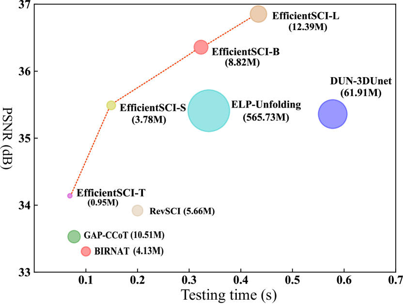
Figure 1: Comparison of reconstruction quality (average PSNR in dB on 6 benchmark grayscale datasets) and testing time of several SOTA deep learning based algorithms. Our proposed EfficientSCI achieves higher reconstruction quality with fewer parameters and shorter testing time.

1 Introduction

Traditional high-speed camera imaging methods usually suffer from high hardware and storage transmission cost. Inspired by compressed sensing (CS) [5, 9], video snapshot compressive imaging (SCI) [45] provides an elegant solution. As shown in Fig. 2, video SCI consists of a hardware encoder and a software decoder. In the encoder part, multiple raw video frames are modulated by different masks and then integrated by the camera to get a compressed measurement, giving low-speed cameras the ability to capture high-speed scenes. For the decoding part, the desired high-speed video is retrieved by the reconstruction algorithm using the captured measurement and masks.

So far, many mature SCI imaging systems [14, 31, 24] have been built, but for the decoding part, there are still many challenges. In particular, although the model-based methods [44, 43, 21] have good flexibility and can reconstruct videos with different resolutions and compression rates, they require long reconstruction time and can only achieve poor reconstruction quality. In order to improve the reconstruction quality and running speed, PnP-FFDNet [46] and PnP-FastDVDnet [47] integrate the pre-trained denoising network into an iterative optimization algorithm. However, they still need a long reconstruction time on large-scale datasets, e.g., PnP-FastDVDNet takes hours to reconstruct a UHD video from a single measurement.

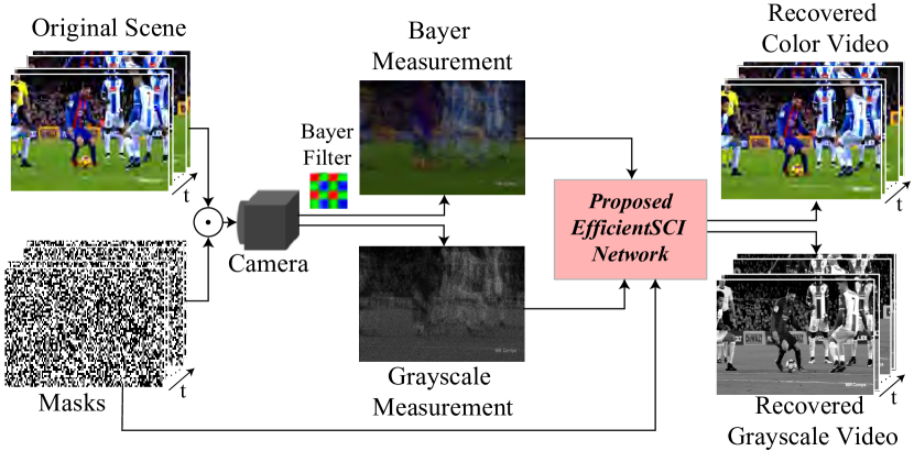
Figure 2: Schematic diagram of grayscale and color video SCI.

By contrast, deep learning based methods [30, 28, 40, 35] have better real-time performance and higher reconstruction quality. For example, BIRNAT [8] uses bidirectional recurrent neural network and generative adversarial method to surpass model-based method DeSCI [21] for the first time. MetaSCI [39] has made some explorations for the model to adapt to different masks, which reduces the model training time. DUN-3DUnet [40] and ELP-Unfolding [42] combine iterative optimization ideas with deep learning models to further improve reconstruction quality. However, due to the high model complexity and insufficient GPU memory, most existing deep learning algorithms cannot train the models required for reconstructing HD or large-scale videos. RevSCI [7] uses a reversible mechanism [2] to reduce the memory used for model training, and can reconstruct HD video with a compression rate up to 24, but the model training time increases exponentially. In addition, the current reconstruction algorithms generally use convolution to establish spatial-temporal correlation. Due to the local connection of convolution, long-term dependencies cannot be well established, and the model cannot reconstruct data with high compression rates.

In summary, model-based methods usually require long reconstruction time and can only achieve poor reconstruction quality. Learning-based methods have high model complexity but cannot be well applied to large-scale color video reconstruction. To address these challenges, we develop an efficient network for video SCI by using dense connections and space-time factorization mechanism. As shown in Fig. 1, our proposed method dramatically outperforms all previous deep learning based reconstruction algorithms in terms of reconstruction quality and running speed with fewer parameters. Our main contributions can be summarized as follows:

• An efficient end-to-end network, dubbed EfficientSCI, is proposed for reconstructing high quality video frames from a snapshot SCI measurement.

• By building hierarchical dense connections within a single residual block, we devise a novel ResDNet block to effectively reduces model computational complexity but enhance the learning ability of the model.

• Based on the space-time factorization mechanism, a Convolution and Transformer hybrid block (CFormer) is built, which can efficiently establish space-time correlation by using convolution in the spatial domain and Transformer in the temporal domain, respectively.

• Experimental results on a large number of simulated and real datasets demonstrate that our proposed method achieves state-of-the-art (SOTA) results and better real-time performance.

2 Related Work

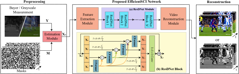
Figure 3: Architecture of the proposed EfficientSCI network and the overall process of color or grayscale video reconstruction. The measurement (${{\bf Y}}$) and masks (${{\bf M}}$) are pre-processed by the estimation module to obtain an estimated ${\bf X}_{e}$, and then feed ${\bf X}_{e}$ into EfficientSCI network to get the desired reconstruction result. (a) ResDNet module with $N$ residual style units. (b) ResDNet block. Inside a residual block, the input features are divided into $S$ parts by the channel split. Each part uses CFormer to efficiently extract spatial-temporal correlation, and employs dense connections to further improve model capacity. For convenience, only the case of $S=4$ is shown here.

CNN and Variants: In the past ten years, models with convolutional neural networks (CNN) as the backbone [20, 13, 15] have achieved excellent results on multiple computer vision tasks [20, 32, 25]. Among them, ResNeXt [41] and Res2Net [11] effectively increases model capacity without increasing model complexity by using grouped convolutions inside residual blocks. DenseNet [15] and CSPNet [34] achieve feature reuse by taking all previous feature maps as input. In video-related tasks, 3D convolution can establish good spatial-temporal correlation and has been widely used in action recognition [18], video super-resolution [26], video inpainting [6] and so on. In previous video SCI reconstruction, RevSCI and DUN-3DUnet greatly improve the reconstruction quality of benchmark grayscale datasets by integrating 3D convolution into the network. However, in complex high-speed scenarios (e.g., crash), since they cannot effectively establish long-term temporal dependencies, the reconstruction quality is still lower than 30 dB. In addition, the excessive use of 3D convolution increases the amount of model parameters, which is not conducive to the application of large-scale and high compression ratio data.

Vision Transformers: Most recently, Vision Transformer (ViT) [10] and its variants [37, 12, 50, 4] have achieved competitive results in computer vision. However, the high computational complexity limits its application in video-related tasks. TimeSformer [3] performs self-attention calculations in time and space respectively, which reduces model complexity and improves model accuracy, but the computational complexity still increases quadratically with the image size. The Video Swin Transformer [23] limits self-attention calculations to local windows but cannot effectively establish long-term temporal dependencies. In addition, a large number of experimental results show that Transformer has higher memory consumption than CNN, and using Transformer in space is not conducive to large-scale video SCI reconstruction. Therefore, through space-time factorization mechanism, using Transformer only in time domain can not only effectively utilize its ability to establish long-term time series dependencies, but also reduce model complexity and memory consumption.

3 Mathematical Model of Video SCI

Fig. 2 briefly describes the flow chart of video SCI. For grayscale video SCI system, the original $B$-frame (grayscale) input video $\{{\bf X}_{m}\}_{m=1}^{B}\in\mathbb{R}^{n_{x}\times{n_{y}}}$ is modulated by pre-defined masks $\{{{\bf M}}\}_{m=1}^{B}\in\mathbb{R}^{n_{x}\times{n_{y}}}$. Then, by compressing across time, the camera sensor captures a compressed measurement ${{\bf Y}}\in\mathbb{R}^{n_{x}\times{n_{y}}}$. The whole process can be expressed as:

$${{\bf Y}}=\textstyle\sum_{m=1}^{B}{{\bf X}_{m}\odot{{\bf M}}_{m}+{\bf Z}},$$ (1)

where $\odot$ denotes the Hadamard (element-wise) multiplication, and ${\bf Z}\in\mathbb{R}^{n_{x}\times{n_{y}}}$ denotes the measurement noise. Eq. (1) can also be represented by a vectorized formulation. Firstly, we vectorize $\boldsymbol{y}=\operatorname{vec}({{\bf Y}})\in\mathbb{R}^{n_{x}{n_{y}}}$, $\boldsymbol{z}=\operatorname{vec}({\bf Z})\in\mathbb{R}^{n_{x}{n_{y}}}$, $\boldsymbol{x}=\left[\boldsymbol{x}_{1}^{\top},\ldots,\boldsymbol{x}^{\top}_{B}\right]^{\top}\in\mathbb{R}^{n_{x}{n_{y}{B}}}$, where $\boldsymbol{x}_{m}=\operatorname{vec}({\bf X}_{m})$. Then, sensing matrix generated by masks can be defined as:

$${{\bf H}}=\left[{\bf D}_{1},\ldots,{\bf D}_{B}\right]\in\mathbb{R}^{n_{x}{n_{y}}\times{n_{x}{n_{y}{B}}}},$$ (2)

where ${\bf D}_{m}=\operatorname{Diag}(\operatorname{vec}({{\bf M}}))\in\mathbb{R}^{n_{x}n_{y}\times n_{x}n_{y}}$ is a diagonal matrix and its diagonal elements is filled by $\operatorname{vec}({{\bf M}})$. Finally, the vectorized expression of Eq. (1) is

$$\boldsymbol{y}={{\bf H}}{\boldsymbol{x}}+\boldsymbol{z}.$$ (3)

For color video SCI system, we use the Bayer pattern filter sensor, where each pixel captures only red (R), blue (B) or green (G) channel of the raw data in a spatial layout such as ‘RGGB’. Since adjacent pixels are different color components, we divide the original measurement ${{\bf Y}}$ into four sub-measurements $\{{{\bf Y}}^{r},{{\bf Y}}^{g1},{{\bf Y}}^{g2},{{\bf Y}}^{b}\}\in\mathbb{R}^{\frac{n_{x}}{2}\times{\frac{n_{y}}{2}}}$ according to the Bayer filter pattern. For color video reconstruction, most of the previous algorithms [48, 46] reconstruct each sub-measurement independently, and then use off-the-shelf demosaic algorithms to get the final RGB color videos. These methods are usually inefficient and have poor reconstruction quality. In this paper, we feed the four sub-measurements simultaneously into the reconstruction network to directly obtain the final desired color video.

4 The Proposed Network

As shown in Fig. 3, in the pre-processing stage of EfficientSCI, inspired by [8, 7], we use the estimation module to pre-process measurement (Y) and masks (M) as follows:

$$\overline{{{\bf Y}}}=\textstyle{{\bf Y}}\oslash\sum_{m=1}^{B}{{{\bf M}}_{m}},\;~{}~{}{\bf X}_{e}=\overline{{{\bf Y}}}\odot{{\bf M}}+\overline{{{\bf Y}}},$$ (4)

where $\oslash$ represents Hadamard (element-wise) division, $\overline{{{\bf Y}}}\in\mathbb{R}^{n_{x}\times{n_{y}}}$ is the normalized measurement, which preserves a certain background and motion trajectory information, and ${\bf X}_{e}\in\mathbb{R}^{n_{x}\times{n_{y}}\times{B}}$ represents the coarse estimate of the desired video. We then take ${\bf X}_{e}$ as the input of the EfficientSCI network to get the final reconstruction result.

EfficientSCI network is mainly composed of three parts: $i)$ feature extraction module, $ii)$ ResDNet module and $iii)$ video reconstruction module. The feature extraction module is mainly composed of three 3D convolutional layers with kernel sizes of $3\times{7}\times{7},3\times{3}\times{3}$ and $3\times{3}\times{3}$ respectively. Among them, each 3D convolution is followed by a LeakyReLU activation function [27], and the spatial stride step size of the final 3D convolution is 2. The spatial resolution of the final output feature map is reduced to half of the input. The feature extraction module effectively maps the input image space to the high-dimensional feature space. The ResDNet module is composed of $N$ ResDNet block (described in Sec. 4.1), which can efficiently explore spatial-temporal correlation. The video reconstruction module is composed of pixelshuffle [33] (mainly restore spatial resolution to input network input size) and three 3D convolution layers (kernel sizes are $3\times{3}\times{3},1\times{1}\times{1}$ and $3\times{3}\times{3}$ respectively), and conducts video reconstruction on the features output by the ResDNet blocks.

4.1 ResDNet Block

Dense connection is an effective way to increase model capacity. Unlike DenseNet, which spans multiple layers, we build a more efficient dense connection within a single residual block. As shown in Fig. 3(b), the input features of the ResDNet block are first divided into $S$ parts along the feature channel dimension. Then, for each part $i=1,\cdots,S$, we use CFormer (described in Section  4.2) to efficiently establish the spatial-temporal correlation. Specifically, for the input of the $i^{th}$ CFormer, we concatenate all the CFormer output features before the $i^{th}$ part with the input features of the $i^{th}$ part and then use a $1\times{1}\times{1}$ convolution to reduce the dimension of the feature channel, which can further reduce the computational complexity. Next, we concatenate all CFormer output features along the feature channel dimension and use a $1\times{1}\times{1}$ convolution to better fuse each part of the information. Given an input ${\bf X}_{r}\in\mathbb{R}^{T\times{H}\times{W}\times{C}}$, ResDNet block can be expressed as:

$${\bf X}_{1},\cdots,{\bf X}_{S}={\rm Split}({\bf X}_{r}),$$

$${{{\bf Y}}}_{1}={\rm CFormer_{1}}({\bf X}_{1}),$$

$${{{\bf Y}}}_{2}={\rm CFormer_{2}}({\rm Conv_{1}}({\rm Concat}([{{{\bf Y}}}_{1},{\bf X}_{2}]))),$$

$$\qquad\qquad\vdots$$

$${{{\bf Y}}}_{S}={\rm CFormer_{S}}({\rm Conv_{1}}({\rm Concat}([{{\bf Y}}_{1},\cdots,{{{\bf Y}}}_{S-1},{\bf X}_{S}]))),$$

$$\hat{{{\bf Y}}}_{r}={\rm Concat}([{{{\bf Y}}}_{1},\cdots,{{{\bf Y}}}_{S}]),$$

$$\hat{{\bf X}}_{r}={\rm Conv_{1}(\hat{{{\bf Y}}}_{r})}+{\bf X}_{r},$$ (5)

where ‘Split’ represents division along the channel, ‘${\rm Conv_{1}}$’ represents a $1\times{1}\times{1}$ convolution operation, ‘Concat’ represents concatenate along the channel and $\hat{{\bf X}}_{r}\in\mathbb{R}^{T\times{H}\times{W}\times{C}}$ represents the output of the ResDNet block. This design has two advantages: $i)$ the features of different levels are aggregated at a more granular level, which improves the representation ability of the model; $ii)$ the model complexity is reduced (shown in Table 6).

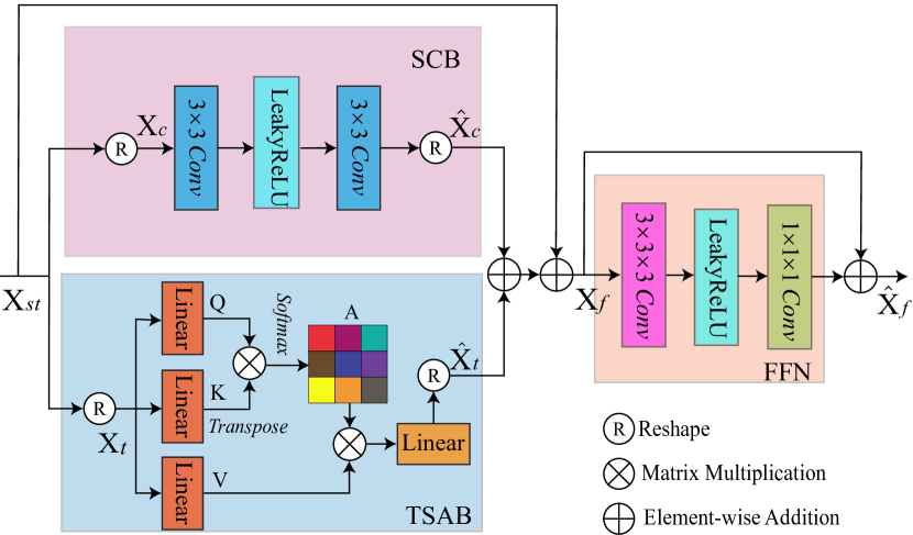
Figure 4: The CFormer block is composed of Spatial Convolution Branch (SCB), Temporal Self-Attention Branch (TSAB) and Feed Forward Network (FFN). For ease of presentation, only the head $N=1$ scenario is described in the TSAB.

4.2 CFormer Block

As shown in Fig. 4, the CFormer block includes three parts: Spatial Convolution Branch (SCB), Temporal Self-Attention Branch (TSAB) and Feed Forward Network (FFN). Based on the space-time factorization mechanism, SCB is used to extract spatial local information, TSAB is used to calculate temporal attention of the feature points at the same spatial position in each frame. After that, FFN is used to further integrate spatial-temporal information.

It is worth noting that in order to make the model flexible to different compression ratios, we introduce zero padding position encoding [17] into CFormer block, instead of the absolute position encoding [10] or relative position encoding [22]. Specifically, we modified the first linear transformation layer in the traditional FFN to a $3\times{3}\times{3}$ convolution with padding size of 1.

Spatial Convolution Branch: 2D convolution can well exploit spatial local correlation and reconstructs more detailed information, and it also enjoys efficient memory consumption and higher operating efficiency, which is suitable for large-scale video reconstruction. Therefore, We only use two $3\times{3}$ 2D convolutions to reconstruct spatial local details in SCB as shown in Fig. 4.

Temporal Self-attention Branch: The local receptive field of convolution makes it difficult to establish long-term dependencies. The global perception ability of Transformer can mitigate this issue. However, the time and memory complexity of traditional Transformers increase quadratically with the image size. To alleviate this problem, following [3, 35], we propose TSAB (shown in Fig. 4), which restricts the self-attention computation to the temporal domain, and its complexity only increase linearly with the image/video size.

In particular, we first reshape the input ${\bf X}_{st}\in\mathbb{R}^{T\times{H}\times{W}\times{\frac{C}{S}}}$ to ${\bf X}_{t}\in\mathbb{R}^{HW\times{T}\times{\frac{C}{S}}}$, and then obtain $query\;({{\bf Q}}\in\mathbb{R}^{HW\times{T}\times{\frac{C}{2S}}})$, $key\;({{\bf K}}\in\mathbb{R}^{HW\times{T}\times{\frac{C}{2S}}})$ and $value\;({{\bf V}}\in\mathbb{R}^{HW\times{T}\times{\frac{C}{2S}}})$ by linearly mapping ${\bf X}_{t}$:

$${{\bf Q}}={\bf X}_{t}{{\bf W}}^{Q},~{}~{}{{\bf K}}={\bf X}_{t}{{\bf W}}^{K},~{}~{}{{\bf V}}={\bf X}_{t}{{\bf W}}^{V},$$ (6)

where $\{{{\bf W}}^{Q},{{\bf W}}^{K},{{\bf W}}^{V}\}\in\mathbb{R}^{\frac{C}{S}\times{\frac{C}{2S}}}$ are projection matrices.

It is worth noting that the output dimension of the projection matrix is reduced to half of the input dimension, further decreasing the computational complexity of TSAB. Then, we respectively divide ${{\bf Q}}$, ${{\bf K}}$, ${{\bf V}}$ into $N$ heads along the feature channel: ${{\bf Q}}=\{{{\bf Q}}_{j}\}_{1}^{N}$, ${{\bf K}}=\{{{\bf K}}_{j}\}_{1}^{N}$, ${{\bf V}}=\{{{\bf V}}_{j}\}_{1}^{N}\in\mathbb{R}^{HW\times{T}\times{\frac{C}{2SN}}}$. For each head $j=1,\cdots,N$, the attention can be calculated as:

$$head_{j}={\bf A}_{j}*{{\bf V}}_{j},$$ (7)

where ${\bf A}_{j}=softmax({{\bf Q}}_{j}{{\bf K}}_{j}^{T}/\sqrt{d})\in\mathbb{R}^{HW\times{T}\times{T}}$ represents an attention map, ${{\bf K}}_{j}^{T}$ represents the transposed matrix of ${{\bf K}}_{j}$ and $d=\frac{C}{2SN}$ is a scaling parameter. Then, we concatenate the outputs of $N$ heads along the feature channel dimension and perform a linear mapping to obtain the final output $\hat{{\bf X}}_{t}\in\mathbb{R}^{T\times{H}\times{W}\times{\frac{C}{S}}}$ of TSAB:

$$\hat{{\bf X}}_{t}={{\bf R}}({{\bf W}}^{P}({\rm Concat}[head_{1},\cdots,head_{N}])),$$ (8)

where ${{\bf W}}^{P}\in\mathbb{R}^{\frac{C}{2S}\times\frac{C}{S}}$ represents projection matrices, and ${{\bf R}}$ is the reshape operator.

Table 1: Computational complexity of several SOTA methods.

Method	Computational Complexity
SCB3D	$\frac{1}{2}HWTK^{3}C^{2}$
G-MSA	$HWTC^{2}+(HWT)^{2}C$
TS-MSA	$2HWTC^{2}+T(HW)^{2}C+HWT^{2}C$
SCB	$\frac{1}{2}HWTK^{2}C^{2}$
TSAB	$\frac{1}{2}HWTC^{2}+\frac{1}{2}HWT^{2}C$

We further analyze the computational complexity of SCB and TSAB, and compare them with 3D convolution and several classic Multi-head Self-Attention (MSA) mechanisms. The results are shown in Table 1, where ‘SCB3D’ represents the replacement of 2D convolution in SCB with 3D convolution and $K$ represents the kernel size , ‘G-MSA’ represents the original global MSA [10], and ‘TS-MSA’ represents the MSA in TimeSformer [3]. It can be observed that the computational complexity of our proposed SCB and TSAB grows linearly with the spatial size $HW$, the computational cost is much less than ‘TS-MSA’ and ‘G-MSA’ (grow quadratically with $HW$). Compared with 3D convolution, since $T$ is generally smaller than $C$, ‘SCB’ and ‘TSAB’ still need less computational cost.

Feed Forward Network: The feed forward network of traditional Transformer usually uses two linear layers and a nonlinear activation function to learn more abstract feature representations. However, in the whole FFN, there is no interaction between the feature points. In order to better integrate the spatial-temporal information and position coding information, we replace the first linear transformation layer in the traditional FFN with a $3\times{3}\times{3}$ convolution.

Given ${\bf X}_{f}\in\mathbb{R}^{T\times{H}\times{W}\times{\frac{C}{2}}}$, FFN can be expressed as:

$$\hat{{\bf X}}_{f}={\bf X}_{f}+{{\bf W}}_{1}(\phi({{\bf W}}_{2}({\bf X}_{f}))),$$ (9)

where ${{\bf W}}_{1},{{\bf W}}_{2}$ represent $1\times{1}\times{1}$ convolution and $3\times{3}\times{3}$ convolution operations respectively, $\phi$ denotes the LeakyReLU non-linearity activation, and $\hat{{\bf X}}_{f}\in\mathbb{R}^{T\times{H}\times{W}\times{\frac{C}{2}}}$ is the output of the FFN.

It should be noted that in the whole CFormer block, we do not use any regularization layers, such as Layer Normalization [1] and Batch Normalization [16]. The experimental results show that removing the regularization layer will not reduce the quality of model reconstruction and can further improve the efficiency of the model.

Table 2: Reconstruction quality and test time (s) using EfficientSCI with different number of channels and blocks.

Model	Channel	Block	PSNR	SSIM	Test time(s)
EfficientSCI-T	64	8	34.22	0.961	0.07
EfficientSCI-S	128	8	35.51	0.970	0.15
EfficientSCI-B	256	8	36.48	0.975	0.31
EfficientSCI-L	256	12	36.92	0.977	0.45

Table 3: Computational complexity and reconstruction quality of several SOTA algorithms on 6 grayscale benchmark datasets.

Method	Params (M)	FLOPs (G)	PSNR	SSIM
BIRNAT	4.13	390.56	33.31	0.951
RevSCI	5.66	766.95	33.92	0.956
DUN-3DUnet	61.91	3975.83	35.26	0.968
ELP-Unfolding	565.73	4634.94	35.41	0.969
EfficientSCI-T	0.95	142.18	34.22	0.961
EfficientSCI-S	3.78	563.87	35.51	0.970
EfficientSCI-B	8.82	1426.38	36.48	0.975
EfficientSCI-L	12.39	1893.72	36.92	0.977

Network Variants: To balance speed and performance of the proposed network, we introduce four different versions of EfficientSCI network, dubbed as EfficientSCI-T, EfficientSCI-S, EfficientSCI-B and EfficientSCI-L standing for Tiny, Small, Base and Large networks, respectively. The network hyper-parameters are shown in Table 2, in which we mainly changed the the number of ResDNet blocks and the number of channels. As shown in Table 3, we also compare model parameters and computational complexity (FLOPs) with several advanced methods. The complexity of our proposed EfficientSCI-T is smaller than that of BIRNAT and RevSCI, and EfficientSCI-L is smaller than that of DUN-3DUnet and ELP-Unfolding.

Table 4: The average PSNR in dB (left entry) and SSIM (right entry) and running time per measurement of different algorithms on 6 benchmark grayscale datasets. The best results are shown in bold and the second-best results are underlined.

Method	Kobe	Traffic	Runner	Drop	Crash	Aerial	Average	Test time(s)
GAP-TV	26.46, 0.885	20.89, 0.715	28.52, 0.909	34.63, 0.970	24.82, 0.838	25.05, 0.828	26.73, 0.858	4.2 (CPU)
PnP-FFDNet	30.50, 0.926	24.18, 0.828	32.15, 0.933	40.70, 0.989	25.42, 0.849	25.27, 0.829	29.70, 0.892	3.0 (GPU)
PnP-FastDVDnet	32.73, 0.947	27.95, 0.932	36.29, 0.962	41.82, 0.989	27.32, 0.925	27.98, 0.897	32.35, 0.942	6.0 (GPU)
DeSCI	33.25, 0.952	28.71, 0.925	38.48, 0.969	43.10, 0.993	27.04, 0.909	25.33, 0.860	32.65, 0.935	6180 (CPU)
BIRNAT	32.71, 0.950	29.33, 0.942	38.70, 0.976	42.28, 0.992	27.84, 0.927	28.99, 0.917	33.31, 0.951	0.10 (GPU)
RevSCI	33.72, 0.957	30.02, 0.949	39.40, 0.977	42.93, 0.992	28.12, 0.937	29.35, 0.924	33.92, 0.956	0.19 (GPU)
GAP-CCoT	32.58, 0.949	29.03, 0.938	39.12, 0.980	42.54, 0.992	28.52, 0.941	29.40, 0.923	33.53, 0.958	0.08 (GPU)
DUN-3DUnet	35.00, 0.969	31.76, 0.966	40.03, 0.980	44.96, 0.995	29.33, 0.956	30.46, 0.943	35.26, 0.968	0.58 (GPU)
ELP-Unfolding	34.41, 0.966	31.58, 0.962	41,16, 0.986	44.99, 0.995	29.65, 0.959	30.68, 0.944	35.41, 0.969	0.34 (GPU)
EfficientSCI-T	33.45, 0.960	29.20, 0.942	39.51, 0.981	43.56, 0.993	29.27, 0.954	30.32, 0.937	34.22, 0.961	0.07 (GPU)
EfficientSCI-S	34.79, 0.968	31.21, 0.961	41.34, 0.986	44.61, 0.994	30.34, 0.965	30.78, 0.945	35.51, 0.970	0.15 (GPU)
EfficientSCI-B	35.76, 0.974	32.30, 0.968	43.05, 0.988	45.18, 0.995	31.13, 0.971	31.50, 0.953	36.48, 0.975	0.31 (GPU)
EfficientSCI-L	36.27, 0.976	32.83, 0.971	43.79, 0.991	45.46, 0.995	31.52, 0.974	31.64, 0.955	36.92, 0.977	0.45 (GPU)

5 Experiment Results

5.1 Datasets

Following BIRNAT [8], we use DAVIS2017 [29] with resolution $480\times{894}$ (480p) as the model training dataset. To verify model performance, we first test the EfficientSCI network on several simulated datasets, including six benchmark grayscale datasets (Kobe, Traffic, Runner, Drop, Crash and Aerial with a size of $256\times{256}\times{8}$), six benchmark mid-scale color datasets (Beauty, Bosphorus, Jockey, Runner, ShakeNDry and Traffic with a size of $512\times{512}\times{3}\times{8}$), and four large-scale datasets (Messi, Hummingbird, Swinger and Football with different sizes and compression ratios). Then we test our model on some real data (including Domino, Water Balloon) captured by a real SCI system [30].

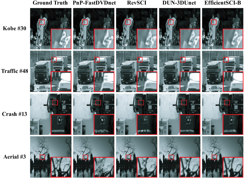
Figure 5: Selected reconstruction frames of simulated grayscale data. Zoom in for better view.

5.2 Implementation Details

We use PyTorch framework with 4 NVIDIA RTX 3090 GPUs for training with random cropping, random scaling, and random flipping for data augmentation, and use Adam [19] to optimize the model with the initial learning rate 0.0001. After iterating for 300 epochs, we adjusted the learning rate to 0.00001 and continued to iterate for 40 epochs to get the final model parameters. The peak-signal-to-noise-ratio (PSNR) and structured similarity index metrics (SSIM) [38] are used as the performance indicators of reconstruction quality.

5.3 Results on Simulation Datasets

5.3.1 Grayscale Simulation Video

We compare our method with SOTA model-based methods (GAP-TV [44], PnP-FFDNet [46], PnP-FastDVDnet [47], DeSCI [21]) and deep learning-based methods (BIRNAT [8], RevSCI [7], GAP-CCoT [36], DUN-3DUnet [40], ELP-Unfolding [42]) on simulated grayscale datasets. Table 4 shows the quantitative comparison results, it can be observed that our proposed EfficientSCI-L can achieve the highest reconstruction quality and has good real-time performance. In particular, the PSNR value of our method surpasses the existing best method ELP-Unfolding by 1.46 dB on average. In addition, our proposed EfficientSCI-T achieves high reconstruction quality while achieving the best real-time performance. It is worth noting that, for a fair comparison, we uniformly test the running time of all deep learning based methods on the same NVIDIA RTX 3090 GPU. Fig. 5 shows the visual reconstruction results of some data. By zooming in some local areas, we can observe that our method can recover sharper edges and more detailed information compared to previous SOTA methods. The mid-scale color results are shown in the SM due to space limitation and our method outperforms previous SOTA by 2.02 dB in PSNR on the benchmark dataset [47].

Table 5: The average PSNR in dB (left entry) and SSIM (middle entry) and test time (minutes) per measurement (right entry) of different algorithms on 4 benchmark large-scale datasets. Best results are in bold.

Dataset	Pixel resolution	GAP-TV	PnP-FFDNet-color	PnP-FastDVDnet-color	EfficientSCI-S
Messi	$1080\times{1920}\times{3}\times{8}$	25.20, 0.874, 0.66	34.28, 0.968, 14.93	34.34, 0.970, 15.94	34.41, 0.973, 0.09
Hummingbird	$1080\times{1920}\times{3}\times{30}$	25.10, 0.750, 20.3	28.79, 0.665, 61.20	31.17, 0.916, 54.00	35.56, 0.952, 0.39
Swinger	$2160\times{3840}\times{3}\times{15}$	22.68, 0.769, 39.2	29.30, 0.934, 138.8	30.57, 0.949, 138.4	31.05, 0.951, 0.62
Football	$1644\times{3840}\times{3}\times{40}$	26.19, 0.858, 83.0	32.70, 0.951, 308.8	32.31, 0.947, 298.1	34.81, 0.964, 1.52

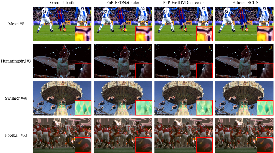
Figure 6: Comparison of reconstruction results of different algorithms on several benchmark large-scale color video simulation datasets.

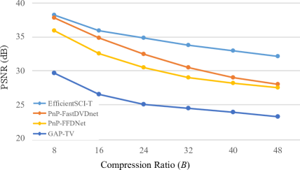
Figure 7: Reconstruction quality (PSNR in dB, higher is better) of different reconstruction algorithms, with varying compression rates $B$ from 8 to 48.

5.3.2 Large-scale Color Simulation Video

Most deep learning based methods, such as BIRNAT [8], DUN-3DUnet [40], cannot be applied to large-scale data reconstruction due to excessive model complexity and GPU memory constraints. RevSCI [7] uses a reversible mechanism and can reconstruct a 24 frames RGB color video with size of $1080\times{1920}\times{3}$, but training the model is extremely slow. GAP-CCoT [36] and ELP-Unfolding [42] only use 2D convolution for reconstruction and thus cannot handle color video data well. Therefore, we only compare with several SOTA model-based methods (GAP-TV [44], PnP-FFDNet-color [46], PnP-FastDVDnet-color [47]) on large-scale color data. Table 5 shows the comparisons between our proposed method and several model-based methods on PSNR, SSIM and test time (in minutes). It can be observed that model-based methods either have long reconstruction time (PnP-FFDNet-color, PnP-FastDVDnet-color) or low reconstruction quality (GAP-TV). Our proposed EfficientSCI-S can achieve higher reconstruction quality and running speed. Especially on UHD color video football ($1644\times{3840}\times{3}\times{40}$), the PSNR value of our method is 2.5 dB higher than PnP-FastDVDnet-color, and the reconstruction time is only $0.5\%$ of it. Fig. 6 shows some visual reconstruction results. By zooming in local areas, we can observe that the reconstruction results of our method are closer to the real value. In addition, our proposed model enjoys high flexibility for different compression ratios, that is, the model trained on low compression ratio data can be directly used for high compression ratio video reconstruction task. To verify this, we test hummingbird data with different compression ratios $B=8,16,24,32,40,48$, and the reconstruction results are shown in Fig. 7. We can observe that our method can be applied to video data with different compression ratios, even when the compression ratio $B$ grows to 48, the PSNR value of EfficientSCI-T model can still reach more than 32 dB. Moreover, our proposed approach surpasses other reconstruction algorithms at all compression ratios.

5.3.3 Ablation Study

To verify the performance of the proposed ResDNet block and CFormer block on the impact of the reconstruction quality, we conduct some ablation experiments. The results are shown in Table 6 and Table 7, we not only compare the reconstruction quality of different models, but also analyze the model parameters and FLOPs. All experiments are conducted on the 6 grayscale benchmark datasets.

Table 6: Ablation study on the ResDNet block without dense connections (left entry) and with dense connections (right entry).

GN	Params	FLOPs	PSNR	SSIM
1	27.40, 27.40	3860.94, 3860.94	35.17, 35.17	0.967, 0.967
2	14.82, 15.08	2211.77, 2246.39	35.09, 36.02	0.966, 0.974
4	8.53, 8.82	1387.33, 1426.38	35.02, 36.48	0.966, 0.975
8	5.38, 5.65	975.39, 1013.45	34.31, 35.68	0.961, 0.971

Table 7: Ablation study on the CFormer block.

SCB	TSAB	Swin	S2-3D	Params (M)	FLOPs (G)	PSNR	SSIM
	✓	✓		2.88	471.03	34.99	0.967
			✓	6.93	999.31	34.93	0.966
✓	✓			3.78	563.87	35.51	0.970

ResDNet Block: We verify the effect of different group numbers (GN) (corresponding to $S$ in Eq. 4.1) and dense connections on the reconstruction quality. As shown in Table 6, the model complexity decreases gradually with the increase of GN, but the reconstruction quality greatly decreases when there are no dense connections in the ResDNet block. By introducing dense connections in the ResDNet block, the reconstruction quality of our proposed method is greatly improved, and a gain of 1.46 dB can be obtained when GN is 4.

CFormer Block: In the CFormer block, we first replace SCB with Swin Transformer (Swin) to verify its effectiveness. Then, we replace SCB and TSAB with two stacked 3D convolutions (S2-3D) to verify the effectiveness of TSAB. As shown in Table 7, compared with Swin Transformer, SCB can bring a 0.52 dB gain. Although the number of parameters and FLOPs have increased, the experimental results show that SCB takes up less memory than the Swin Transformer, which is very important for large-scale and high compression ratio data. Please refer to more detailed analysis in SM. Compared with SCB and TSAB, S2-3D not only increases model parameters and FLOPs by $83\%$ and $77\%$ respectively, but also reduces the PSNR value by 0.58 dB, which verifies the necessity of using space-time factorization and TSAB.

Number of Channels and Blocks: Table 2 shows that the quality of model reconstruction increases with the number of channels and blocks. However, the amount of parameters and FLOPs also increase (see Table  3), resulting in a degradation in the real-time performance of the model.

Figure 8: Reconstruction results of different algorithms on Domino real data with compression rate $B=10$.

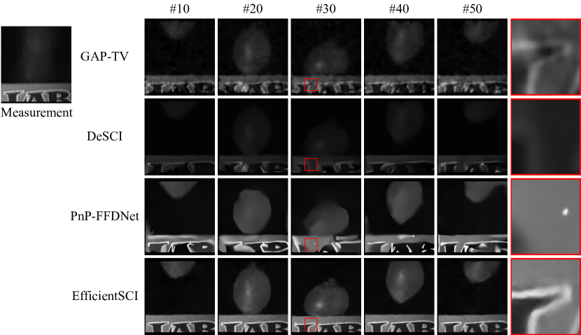
Figure 9: Reconstruction results of different algorithms on Water Balloon real data with compression rate $B=50$.

5.4 Results on Real Video SCI Data

We further test our method on real data. Fig. 8 and Fig. 9 show the reconstruction results of multiple algorithms on two public data (Domino, Water Balloon), we can see that our method can reconstruct clearer details and edges. Specifically, we can clearly recognize the letters on the Domino. Even with a high compression ratio ($B=50$), our proposed method can still reconstruct clear foreground and background information (shown in Fig. 9).

6 Conclusions and Future Work

This paper proposes an efficient end-to-end video SCI reconstruction network, dubbed EfficientSCI, which achieves the state-of-the-art performance on simulated data and real data, significantly surpassing the previous best reconstruction algorithms with high real-time performance. In addition, we show for the first time that an UHD color video with high compression rate can be reconstructed using a deep learning based method. For future work, we consider applying EfficientSCI Network to more SCI reconstruction tasks, such as spectral SCI [49, 4].

References

- [1] Jimmy Lei Ba, Jamie Ryan Kiros, and Geoffrey E Hinton. Layer normalization. arXiv preprint arXiv:1607.06450, 2016.
- [2] Jens Behrmann, Will Grathwohl, Ricky TQ Chen, David Duvenaud, and Jörn-Henrik Jacobsen. Invertible residual networks. In International Conference on Machine Learning, pages 573–582. PMLR, 2019.
- [3] Gedas Bertasius, Heng Wang, and Lorenzo Torresani. Is space-time attention all you need for video understanding? In ICML, volume 2, page 4, 2021.
- [4] Yuanhao Cai, Jing Lin, Xiaowan Hu, Haoqian Wang, Xin Yuan, Yulun Zhang, Radu Timofte, and Luc Van Gool. Mask-guided spectral-wise transformer for efficient hyperspectral image reconstruction. In Proceedings of the IEEE/CVF Conference on Computer Vision and Pattern Recognition, pages 17502–17511, 2022.
- [5] Emmanuel J Candès, Justin Romberg, and Terence Tao. Robust uncertainty principles: Exact signal reconstruction from highly incomplete frequency information. IEEE Transactions on information theory, 52(2):489–509, 2006.
- [6] Ya-Liang Chang, Zhe Yu Liu, Kuan-Ying Lee, and Winston Hsu. Free-form video inpainting with 3d gated convolution and temporal patchgan. In Proceedings of the IEEE/CVF International Conference on Computer Vision, pages 9066–9075, 2019.
- [7] Ziheng Cheng, Bo Chen, Guanliang Liu, Hao Zhang, Ruiying Lu, Zhengjue Wang, and Xin Yuan. Memory-efficient network for large-scale video compressive sensing. In Proceedings of the IEEE/CVF Conference on Computer Vision and Pattern Recognition, pages 16246–16255, 2021.
- [8] Ziheng Cheng, Ruiying Lu, Zhengjue Wang, Hao Zhang, Bo Chen, Ziyi Meng, and Xin Yuan. BIRNAT: Bidirectional recurrent neural networks with adversarial training for video snapshot compressive imaging. In European Conference on Computer Vision, pages 258–275. Springer, 2020.
- [9] David L Donoho. Compressed sensing. IEEE Transactions on information theory, 52(4):1289–1306, 2006.
- [10] Alexey Dosovitskiy, Lucas Beyer, Alexander Kolesnikov, Dirk Weissenborn, Xiaohua Zhai, Thomas Unterthiner, Mostafa Dehghani, Matthias Minderer, Georg Heigold, Sylvain Gelly, et al. An image is worth 16x16 words: Transformers for image recognition at scale. In International Conference on Learning Representations, 2020.
- [11] Shang-Hua Gao, Ming-Ming Cheng, Kai Zhao, Xin-Yu Zhang, Ming-Hsuan Yang, and Philip Torr. Res2net: A new multi-scale backbone architecture. IEEE transactions on pattern analysis and machine intelligence, 43(2):652–662, 2019.
- [12] Kai Han, Yunhe Wang, Hanting Chen, Xinghao Chen, Jianyuan Guo, Zhenhua Liu, Yehui Tang, An Xiao, Chunjing Xu, Yixing Xu, et al. A survey on vision transformer. IEEE Transactions on Pattern Analysis and Machine Intelligence, 2022.
- [13] Kaiming He, Xiangyu Zhang, Shaoqing Ren, and Jian Sun. Deep residual learning for image recognition. In Proceedings of the IEEE conference on computer vision and pattern recognition, pages 770–778, 2016.
- [14] Yasunobu Hitomi, Jinwei Gu, Mohit Gupta, Tomoo Mitsunaga, and Shree K Nayar. Video from a single coded exposure photograph using a learned over-complete dictionary. In 2011 International Conference on Computer Vision, pages 287–294. IEEE, 2011.
- [15] Gao Huang, Zhuang Liu, Laurens Van Der Maaten, and Kilian Q Weinberger. Densely connected convolutional networks. In Proceedings of the IEEE conference on computer vision and pattern recognition, pages 4700–4708, 2017.
- [16] Sergey Ioffe and Christian Szegedy. Batch normalization: Accelerating deep network training by reducing internal covariate shift. In International conference on machine learning, pages 448–456. PMLR, 2015.
- [17] Md Amirul Islam, Sen Jia, and Neil DB Bruce. How much position information do convolutional neural networks encode? arXiv preprint arXiv:2001.08248, 2020.
- [18] Shuiwang Ji, Wei Xu, Ming Yang, and Kai Yu. 3d convolutional neural networks for human action recognition. IEEE transactions on pattern analysis and machine intelligence, 35(1):221–231, 2012.
- [19] Diederik P Kingma and Jimmy Ba. Adam: A method for stochastic optimization. arXiv preprint arXiv:1412.6980, 2014.
- [20] Alex Krizhevsky, Ilya Sutskever, and Geoffrey E Hinton. Imagenet classification with deep convolutional neural networks. Advances in neural information processing systems, 25:1097–1105, 2012.
- [21] Yang Liu, Xin Yuan, Jinli Suo, David J Brady, and Qionghai Dai. Rank minimization for snapshot compressive imaging. IEEE transactions on pattern analysis and machine intelligence, 41(12):2990–3006, 2018.
- [22] Ze Liu, Yutong Lin, Yue Cao, Han Hu, Yixuan Wei, Zheng Zhang, Stephen Lin, and Baining Guo. Swin transformer: Hierarchical vision transformer using shifted windows. In Proceedings of the IEEE/CVF International Conference on Computer Vision, pages 10012–10022, 2021.
- [23] Ze Liu, Jia Ning, Yue Cao, Yixuan Wei, Zheng Zhang, Stephen Lin, and Han Hu. Video swin transformer. In Proceedings of the IEEE/CVF Conference on Computer Vision and Pattern Recognition, pages 3202–3211, 2022.
- [24] Patrick Llull, Xuejun Liao, Xin Yuan, Jianbo Yang, David Kittle, Lawrence Carin, Guillermo Sapiro, and David J Brady. Coded aperture compressive temporal imaging. Optics express, 21(9):10526–10545, 2013.
- [25] Jonathan Long, Evan Shelhamer, and Trevor Darrell. Fully convolutional networks for semantic segmentation. In Proceedings of the IEEE conference on computer vision and pattern recognition, pages 3431–3440, 2015.
- [26] Jianping Luo, Shaofei Huang, and Yuan Yuan. Video super-resolution using multi-scale pyramid 3d convolutional networks. In Proceedings of the 28th ACM International Conference on Multimedia, pages 1882–1890, 2020.
- [27] Andrew L Maas, Awni Y Hannun, Andrew Y Ng, et al. Rectifier nonlinearities improve neural network acoustic models. In Proc. icml, volume 30, page 3. Citeseer, 2013.
- [28] Ziyi Meng, Shirin Jalali, and Xin Yuan. GAP-net for snapshot compressive imaging. arXiv preprint arXiv:2012.08364, 2020.
- [29] Jordi Pont-Tuset, Federico Perazzi, Sergi Caelles, Pablo Arbeláez, Alex Sorkine-Hornung, and Luc Van Gool. The 2017 davis challenge on video object segmentation. arXiv preprint arXiv:1704.00675, 2017.
- [30] Mu Qiao, Ziyi Meng, Jiawei Ma, and Xin Yuan. Deep learning for video compressive sensing. APL Photonics, 5(3):30801, 2020.
- [31] Dikpal Reddy, Ashok Veeraraghavan, and Rama Chellappa. P2C2: Programmable pixel compressive camera for high speed imaging. In CVPR 2011, pages 329–336. IEEE, 2011.
- [32] Joseph Redmon, Santosh Divvala, Ross Girshick, and Ali Farhadi. You only look once: Unified, real-time object detection. In Proceedings of the IEEE conference on computer vision and pattern recognition, pages 779–788, 2016.
- [33] Wenzhe Shi, Jose Caballero, Ferenc Huszár, Johannes Totz, Andrew P Aitken, Rob Bishop, Daniel Rueckert, and Zehan Wang. Real-time single image and video super-resolution using an efficient sub-pixel convolutional neural network. In Proceedings of the IEEE conference on computer vision and pattern recognition, pages 1874–1883, 2016.
- [34] Chien-Yao Wang, Hong-Yuan Mark Liao, Yueh-Hua Wu, Ping-Yang Chen, Jun-Wei Hsieh, and I-Hau Yeh. Cspnet: A new backbone that can enhance learning capability of cnn. In Proceedings of the IEEE/CVF conference on computer vision and pattern recognition workshops, pages 390–391, 2020.
- [35] Lishun Wang, Miao Cao, Yong Zhong, and Xin Yuan. Spatial-temporal transformer for video snapshot compressive imaging. IEEE Transactions on Pattern Analysis and Machine Intelligence, 2022.
- [36] Lishun Wang, Zongliang Wu, Yong Zhong, and Xin Yuan. Snapshot spectral compressive imaging reconstruction using convolution and contextual transformer. Photonics Research, 10(8):1848–1858, 2022.
- [37] Wenhai Wang, Enze Xie, Xiang Li, Deng-Ping Fan, Kaitao Song, Ding Liang, Tong Lu, Ping Luo, and Ling Shao. Pyramid vision transformer: A versatile backbone for dense prediction without convolutions. In Proceedings of the IEEE/CVF International Conference on Computer Vision, pages 568–578, 2021.
- [38] Zhou Wang, Alan C Bovik, Hamid R Sheikh, and Eero P Simoncelli. Image quality assessment: from error visibility to structural similarity. IEEE transactions on image processing, 13(4):600–612, 2004.
- [39] Zhengjue Wang, Hao Zhang, Ziheng Cheng, Bo Chen, and Xin Yuan. MetaSCI: Scalable and adaptive reconstruction for video compressive sensing. In Proceedings of the IEEE/CVF Conference on Computer Vision and Pattern Recognition, pages 2083–2092, 2021.
- [40] Zhuoyuan Wu, Jian Zhang, and Chong Mou. Dense deep unfolding network with 3D-CNN prior for snapshot compressive imaging. In Proceedings of the IEEE/CVF International Conference on Computer Vision, pages 4892–4901, 2021.
- [41] Saining Xie, Ross Girshick, Piotr Dollár, Zhuowen Tu, and Kaiming He. Aggregated residual transformations for deep neural networks. In Proceedings of the IEEE conference on computer vision and pattern recognition, pages 1492–1500, 2017.
- [42] Chengshuai Yang, Shiyu Zhang, and Xin Yuan. Ensemble learning priors driven deep unfolding for scalable video snapshot compressive imaging. In IEEE European Conference on Computer Vision (ECCV), 2022.
- [43] Jianbo Yang, Xuejun Liao, Xin Yuan, Patrick Llull, David J Brady, Guillermo Sapiro, and Lawrence Carin. Compressive sensing by learning a Gaussian mixture model from measurements. IEEE Transactions on Image Processing, 24(1):106–119, 2014.
- [44] Xin Yuan. Generalized alternating projection based total variation minimization for compressive sensing. In 2016 IEEE International Conference on Image Processing (ICIP), pages 2539–2543. IEEE, 2016.
- [45] Xin Yuan, David J Brady, and Aggelos K Katsaggelos. Snapshot compressive imaging: Theory, algorithms, and applications. IEEE Signal Processing Magazine, 38(2):65–88, 2021.
- [46] Xin Yuan, Yang Liu, Jinli Suo, and Qionghai Dai. Plug-and-play algorithms for large-scale snapshot compressive imaging. In Proceedings of the IEEE/CVF Conference on Computer Vision and Pattern Recognition, pages 1447–1457, 2020.
- [47] Xin Yuan, Yang Liu, Jinli Suo, Fredo Durand, and Qionghai Dai. Plug-and-play algorithms for video snapshot compressive imaging. IEEE Transactions on Pattern Analysis Machine Intelligence, (01):1–1, 2021.
- [48] Xin Yuan, Patrick Llull, Xuejun Liao, Jianbo Yang, David J Brady, Guillermo Sapiro, and Lawrence Carin. Low-cost compressive sensing for color video and depth. In Proceedings of the IEEE Conference on Computer Vision and Pattern Recognition, pages 3318–3325, 2014.
- [49] Xin Yuan, Tsung-Han Tsai, Ruoyu Zhu, Patrick Llull, David Brady, and Lawrence Carin. Compressive hyperspectral imaging with side information. IEEE Journal of selected topics in Signal Processing, 9(6):964–976, 2015.
- [50] Syed Waqas Zamir, Aditya Arora, Salman Khan, Munawar Hayat, Fahad Shahbaz Khan, and Ming-Hsuan Yang. Restormer: Efficient transformer for high-resolution image restoration. In Proceedings of the IEEE/CVF Conference on Computer Vision and Pattern Recognition, pages 5728–5739, 2022.