Rate-Limited Quantum-to-Classical Optimal Transport in Finite and Continuous-Variable Quantum Systems

Abstract

We consider the rate-limited quantum-to-classical optimal transport in terms of output-constrained rate-distortion coding for both finite-dimensional and continuous-variable quantum-to-classical systems with limited classical common randomness. The main coding theorem provides a single-letter characterization of the achievable rate region of a lossy quantum measurement source coding for an exact construction of the destination distribution (or the equivalent quantum state) while maintaining a threshold of distortion from the source state according to a generally defined distortion observable. The constraint on the output space fixes the output distribution to an IID predefined probability mass function. Therefore, this problem can also be viewed as information-constrained optimal transport which finds the optimal cost of transporting the source quantum state to the destination classical distribution via a quantum measurement with limited communication rate and common randomness.

We develop a coding framework for continuous-variable quantum systems by employing a clipping projection and a dequantization block and using our finite-dimensional coding theorem. Moreover, for the Gaussian quantum systems, we derive an analytical solution for rate-limited Wasserstein distance of order 2, along with a Gaussian optimality theorem, showing that Gaussian measurement optimizes the rate in a system with Gaussian quantum source and Gaussian destination distribution. The results further show that in contrast to the classical Wasserstein distance of Gaussian distributions, which corresponds to an infinite transmission rate, in the Quantum Gaussian measurement system, the optimal transport is achieved with a finite transmission rate due to the inherent noise of the quantum measurement imposed by Heisenberg’s uncertainty principle.

Keywords: quantum information; quantum optimal transport; rate-limited optimal transport; continuous variable quantum; Gaussian quantum system; Gaussian observables; Wasserstein distance; quantum source coding;

1 Introduction

1.1 Overview of Recent Works

The goal of optimal transport is to map a source probability measure into a destination one with the minimum possible cost [1, 2]. Let $X$ be a random variable in the source probability space $(\mathcal{X},\mathcal{F}_{\mathcal{X}},P_{X})$, where $\mathcal{X}$ is the support, $\mathcal{F}_{\mathcal{X}}$ is the event space defined by the $\sigma$-algebra of sets on $\mathcal{X}$, and $P_{X}$ is the probability measure. Let $Y$ be a random variable with the target probability space $(\mathcal{Y},\mathcal{F}_{\mathcal{Y}},P_{Y})$. The optimal transport problem aims at finding an optimal mapping $f:\mathcal{X}\to\mathcal{Y}$ that minimizes the expectation of the transportation cost $c(x,y)$ [3]. However, as such deterministic mappings do not exist in many cases, one has to resort to stochastic channels to transform the source distribution to the target distribution. Thus the problem boils down to finding the optimal coupling $\pi^{*}\in\mathcal{P}(\mathcal{X}\times\mathcal{Y})$ of marginal distributions $P_{X}$ and $P_{Y}$ that minimizes the transportation cost [4]:

$$\pi^{*}=\operatorname*{argmin}_{\pi\in\mathcal{P}(\mathcal{X}\times\mathcal{Y})} \int_{\mathcal{X}\times\mathcal{Y}}c(x,y)\pi(dx,dy),$$

subject to $\int_{\mathcal{X}\times B_{\mathcal{Y}}}\;\pi(dx,dy)=P_{Y}(B_{\mathcal{Y}})$, and $\int_{B_{\mathcal{X}}\times\mathcal{Y}}\pi(dx,dy)=P_{X}(B_{\mathcal{X}})$, for any $B_{\mathcal{X}}\in\mathcal{F}_{\mathcal{X}}$ and $B_{\mathcal{Y}}\in\mathcal{F}_{\mathcal{Y}}$. For a metric space $(\mathcal{X}\times\mathcal{Y},d)$, and the cost given by $d^{p}$, for some $p\geq 1$, Wasserstein $p$-distance between the two probability measures $P_{X}$ and $P_{Y}$ is defined as the $p$-th power of the optimal transportation cost [2, 5, 3, 4]. This problem has been studied extensively in the literature with applications in many areas such as information theory, machine learning and statistical inference [6, 1].

The lossy source-coding problem in information theory aims to determine the minimum required rate for compressing a given source in asymptotically large blocks so that it can be reconstructed to meet a prescribed distortion constraint. The fundamental trade-off between the asymptotic compression rate and the reconstruction distortion is given by the rate-distortion function [7]. A single-letter characterization of the optimal rate-distortion trade-off was provided by Shannon [8]. The concept of simulating a channel was considered in the classical setting by Cuff with the notion of coordination capacity [9, 10], and the problem of distributed channel synthesis [11]. Cuff provided an exact characterization of the associated performance limits. A closely related problem, known as Output-Constrained (OC) lossy source coding was considered in [12, 13], and the corresponding performance limits were characterized. This problem has recently found applications in multiple areas [14, 15, 16, 17, 18]. In contrast to distributed channel synthesis which attempts to simulate a fixed channel, in OC lossy source coding, only the output distribution of the reconstruction is constrained. Moreover, in the latter, the n-letter output distribution has to satisfy an exact product form of the desired single-letter distribution, whereas, in the former, it is only constrained to be close to this product form in variational distance. This renders the problem intimately connected to optimal transport.

In [19], the authors formally introduced the problem of Information-Constrained Optimal Transport by imposing an additional constraint on coupling $\pi$ in the form of a threshold on the mutual information between $X$ and $Y$, and established an upper bound on the information-constrained Wasserstein distance by generalizing Talagrand’s transportation cost inequality. It is worth noting that the information-cost function in [19] is equivalent to the rate-distortion function of OC lossy source coding with unlimited common randomness [12]. The protocol associated with this source coding problem provides an operational significance to the information constraint in [19], which can be interpreted as the optimal transport problem when the communication rate between the source and the destination is limited. We refer to this problem as Rate-Limited Optimal Transport (RLOT).

The quantum version of the optimal transport problem has also been investigated in recent years [20, 21, 22, 23, 24]. In [22], the authors proposed a generalization of the quantum Wasserstein distance of order 2 and proved that it satisfies the triangle inequality. They further showed that the associated quantum optimal transport schemes are in one-to-one correspondence with the quantum channels, and in the case of quantum thermal states, the optimal transport schemes can be realized by quantum Gaussian attenuators/amplifiers. In [24], the quantum Wasserstein distance of order 1 was introduced, and several quantum measure concentration inequalities were established.

The topic of rate-distortion theory has also drawn significant attention in the field of quantum information theory. In an early attempt, Barnum [25] conjectured a lower bound on the rate-distortion function for a quantum channel with entanglement fidelity as the distortion measure, based on the coherent information quantity. His lower bound was later proved to be not tight in [26]. The authors established the quantum rate-distortion theorems for both entanglement-assisted and unassisted systems in terms of quantum information quantities such as entanglement of purification and quantum mutual information. The key analysis in [26] rely on the reverse Shannon theorem [27], which addresses the problem of simulating a noisy channel with the help of a noiseless channel, or more generally, simulating one noisy channel with another noisy channel.

In [28], Winter introduced the notion of information in quantum measurements and established the measurement compression theorem, which delineates the required classical rate and common randomness to faithfully simulate a measurement $\Lambda$ for an input state $\rho$. In [29], variants of this measurement compression theorem were studied for the case of non-feedback simulation and the case with the presence of quantum side information. Further, in [30], Datta et. al. invoked this measurement compression theorem to give a proof of the quantum-to-classical (QC) rate-distortion theorem. This idea of measurement simulation was further extended to distributed measurement simulation for composite quantum states in [31, 32], where the required classical rates and common randomness to faithfully simulate a bipartite state $\rho_{AB}$ using distributed measurements are characterized.

Most of these works provide their coding theorems only for finite-dimensional quantum systems. The problems of measurement compression, the quantum rate distortion, and the reverse Shannon theorem have not been addressed in the continuous variable quantum systems. The key analytical tools that form the basis of these works such as operator Chernoff bounds [33] and one-shot quantum covering lemma [34] have not been studied in the continuous-variable quantum systems. However, the problems of channel capacity of quantum Gaussian states, and accessible information of Gaussian quantum states have been studied extensively [35, 36, 37].

1.2 Contributions

The present paper introduces the QC Rate-Limited Optimal Transport problem involving the measurement of a quantum source to produce a classical outcome with the desired distribution. The cost associated with this transformation is measured by a distortion observable. The system avails limited-rate classical communication and common randomness resources. We establish a single-letter characterization of the achievable rate region of the measurement protocols acting on the quantum source state for the construction of a prescribed destination classical distribution with a specific tolerance for distortion (see Theorem 1). We further consider the QC RLOT problem for the Continuous-Variable (CV) quantum systems and characterize the associated performance limits with the development of a novel continuous measurement coding protocol (see Theorem 2). Our work enables the generalization of quantum optimal transport to the Rate-Limited (RL) setting as well as the generalization of classical information-constrained optimal transport to the quantum setting. Moreover, the analysis of the CV quantum systems is also one of the key contributions of this paper (Section 3).

In particular, we provide a detailed analysis of quantum-to-classical RLOT for the case of qubit source state and entanglement fidelity distortion measure (see [25, 26]); the minimum transportation cost is explicitly characterized and is shown to be achievable with a finite transmission rate (see Theorem 3 and 4). We further provide an evaluation of the optimal performance limit for the Gaussian QC systems with unlimited common randomness using a quadratic distortion observable constructed from canonical quadrature operators. First, we develop a Gaussian measurement optimality theorem (see Theorem 5) which shows for a continuous QC system with a Gaussian quantum source and Gaussian destination distribution, the RLOT is a Gaussian measurement. Moreover, a detailed analytical formulation provides the parameters of the optimal Gaussian measurement. In this special case with unlimited common randomness, the RL optimal transportation cost corresponds to the RL Wasserstein 2-distance between the quantum source state and the classical outcome distribution. In stark contrast to the classical Gaussian systems, in the Gaussian QC system, the QC Wasserstein distance is attainable at a finite communication rate. This is a direct consequence of the Heisenberg uncertainty principle and the fact that the measurement noise cannot be made smaller than a threshold [38, 39].

We would also like to mention some key differences between our source coding theorem and other works. Specifically, in comparison to [30], our work on finite-dimensional systems (Section 2), has the additional constraint that the output must follow a predetermined distribution in the exact IID format. This provides a multi-letter protocol that governs the optimal transportation of a quantum source state to a target distribution, through a RL classical channel and with limited common randomness. In contrast to the conventional rate-distortion theorem for which the common randomness provides no performance improvements, in this problem, the common randomness can help reduce the communication rate by providing the extra randomness required to ensure the output has the desired IID distribution.

1.3 Prospective Applications

The QC RLOT problem, besides its theoretical significance, has possible applications in some practical quantum systems. In this work, we study the systems in which, Alice has many copies of a quantum source and has a description of the source in terms of its density operator. Alice has the freedom to perform any sort of measurement she wants on the copies of quantum source states. The goal is to have a compressed classical approximation of the quantum source (with respect to some distortion measure) while requiring this classical approximation to have a specific IID distribution.

To understand the significance of this output constraint, we first look into the benefits of these output-preserved compressions in the classical systems described in [15, 12, 13, 40]. Specifically, the following issues occur in conventional rate-distortion codings and quantization systems: (I) Discontinuities emerge within the range of outcome values, presenting as discrete steps in the outcomes. (II) In specific setups, the reconstruction assigns null values to some parts of the signal. For the example of Gaussian systems with mean-squared error distortion measure, the problem reduces to reverse waterfilling which produces null values at the tails of the Gaussian spectrum. (III) In the extreme case of zero communications, the output would generate constant null values even if it has some statistical information about the source. To combat these issues, in the classical systems, randomized (dithered) uniform quantizers were used to add some random noise to the signal before the quantization which resulted in better reconstructions that avoided nullified tails or discrete steps [12, 40]. These dithered forms of quantization were studied with their benefits in both uniform quantizers and entropy-coded quantizers in [41, 42, 43, 44, 45].

Using a similar idea of dithering, [40, 13] provided the distribution-preserving quantizers which ensure that the reconstructed signal has the exact distribution as the source. This technique has been shown to be very effective in maintaining the perceptional quality of the voice and image codings. Especially, with the compressors using generative adversarial networks (GAN) which have discriminator networks designed to perceptually distinguish between the source and reconstruction [46, 47, 48, 13].

Furthermore, the Wasserstein distance satisfactorily addressed the problem of vanishing gradient in the training that afflicted classical GANs trained with other distance measures such as total variation or Jensen-Shannon divergence [49]. In quantum GAN systems, it is suggested in several works [50, 51, 24] that the quantum Wasserstein may address similar issues. Hence, the choice of Wasserstein distance as the loss function for these GAN models relates them to the rate-limited optimal transport problem, which was alluded to earlier in the introduction.

In our QC Gaussian measurement OC rate-distortion problem, the Gaussian optimality Theorem 5 basically shows that the OC rate-distortion function can be modeled with a Gaussian measurement with a specific inherent noise independent of the source. This is equivalent to a similar observation in the classical conventional systems that the dithered quantizer can be modeled using additive Gaussian noise [45]. In the light of these results, the QC rate-limited optimal transport problem can find application in analyzing the recently emerging quantum-classical GAN systems where quantum sources are used to generate classical data (image, voice, etc) as described in [52, 53, 54, 55, 56].

The definition of the QC Wasserstein distance and rate-limited QC Wasserstein distance provided in Definition 5.2 may lead to new measure concentration inequalities in the QC framework. For example, in the classical systems, an information-constrained OT inequality is provided in [19], which both sharpens Talagrand’s inequality and extends that inequality to the rate-limited setting. Then following Marton’s approach (blowing-up lemma) [6], the authors obtained new measure concentration inequalities. Similarly, in the quantum setting, a quantum version of the Gaussian concentration inequality was provided in [24] based on the quantum Wasserstein distance of order 1 introduced therein. Therefore, we expect similar development of the optimal transport inequalities and concentration inequalities based on the introduced rate-limited QC Wasserstein distance. These inequalities in the classical setting were further used by [19, 57] to prove a strong data processing inequality which further provides an upper bound on the capacity of primitive relay channels. These results are also expected to be extended to the quantum-classical systems which can have similar applications in analyzing the quantum relay channels, for example, see [58].

The contents of this paper are organized as follows. Finite dimensional QC systems are addressed in Section 2 with the statement of the coding theorem, the proof of the achievability and the proof of converse part, are given in Sections 2.2, 2.3 and 2.4, respectively. We develop the coding theorem of CV quantum systems in Section 3. Specifically, we introduce the continuity theorems that are needed for generalizing the definitions of measurement systems to continuous Hilbert spaces in Section 3.1, state the coding theorem for continuous Hilbert spaces in Section 3.2, and prove the achievability part in Section 3.3. In Section 4, we consider the case of qubit measurement systems with unlimited common randomness, for which a detailed analysis of RLOT is provided. The Gaussian measurement systems are analyzed in Section 5 which introduces the rate-limited QC 2nd-order Wasserstein distance. Finally, proofs of the important theorems and lemmas are provided in the appendices.

1.4 Notation

Let $\mathcal{H}_{A}$ denote the separable Hilbert space of system $A$. Further, Let $\mathcal{L}(\mathcal{H})$ be the set of linear operators on $\mathcal{H}$, and $\mathcal{G}(\mathcal{H})\subset\mathcal{L}(\mathcal{H})$ be the set of all density operators on $\mathcal{H}$. A density operator $\rho^{A}\in\mathcal{G}(\mathcal{H}_{A})$ in Hilbert space $A$ is denoted by the superscript $A$. Moreover, a composite density operator $\tau^{AB}\in\mathcal{G}(\mathcal{H}_{A}\otimes\mathcal{H}_{B})$ is defined over the tensor product Hilbert space of $\mathcal{H}_{A}\otimes\mathcal{H}_{B}$. The trace norm is defined for an operator $P\in\mathcal{L}(\mathcal{H})$ by $\norm{P}_{1}=\mathrm{Tr}\big{[}\sqrt{P^{\dagger}P}\big{]}$. Also, $\mathcal{QN}(m_{X},\Sigma_{X})$ denotes the quantum Gaussian state with mean vector $m_{X}$ and covariance matrix $\Sigma_{X}$. A sequence of $n$ samples taking values in a set $\mathcal{X}$ is expressed by the $n$ superscript and each sample by a subscript, $v^{n}=\{v_{1},v_{2},\cdots,v_{n}\}$. The tensor product of $n$ Hilbert spaces is denoted as $\mathcal{H}_{A_{1}}\otimes\mathcal{H}_{A_{2}}\otimes\cdots\otimes\mathcal{H}_{A_{n}}$. The composite density operator of the state of $n$ systems is denoted by $\rho^{A^{n}}$, where the local state of the $i$-th system is given by $\rho^{A_{i}}$. The term $d_{TV}(P,Q)$ is the total variation distance of between distributions $P$ and $Q$. The trace of a matrix object is denoted by $\mathrm{Sp}\left(.\right)$, as opposed to $\Tr{.}$, the trace on a Hilbert space.

2 Finite Dimensional Quantum Systems

The system is comprised of an n-letter memoryless source with its product state $\rho^{\otimes n}$ as the input of an encoder on Alice’s side, where $\rho$ is a density operator defined on a Hilbert space $\mathcal{H}_{A}$. On Bob’s side, we have the reconstruction Hilbert space $\mathcal{H}_{X}$, representing the classical outcomes as quantum registered classical states, with an orthonormal basis indexed by a finite set $\mathcal{X}$. We also let the quantum state $R$ denote the reference of the source with the associated Hilbert space $\mathcal{H}_{R}$ with $\mbox{dim}(\mathcal{H}_{R})=\mbox{dim}(\mathcal{H}_{A})$. The composite state $\ket{\Psi_{\rho}}^{RA}$ of the source $\rho^{A}$ and the reference is obtained by the canonical purification [33, 29, 28]. The corresponding density operator of this purified state is denoted by $\Psi_{\rho}^{RA}$.

2.1 System Model and Problem Formulation

2.1.1 Distortion Measure

The distortion measure between two systems $R$ and $X$ is defined in the general form using a distortion observable $\Delta_{RX}>0$ defined on $\mathcal{H}_{R}\otimes\mathcal{H}_{X}$ for the single-letter composite state $\tau^{RX}$, as described in [30]:

$$d(\Delta_{RX},\tau^{RX}):=\Tr{\Delta_{RX}\tau^{RX}}.$$ (1)

Then, having an n-letter composite state $\tau^{R^{n}X^{n}}$, and the distortion observable for each $i$-th system defined as $\Delta_{R_{i}X_{i}}$, the average n-letter distortion is defined as

$$d_{n}(\Delta^{(n)},\tau^{R^{n}X^{n}}) :=\Tr{\Delta^{(n)}\tau^{R^{n}X^{n}}}=\frac{1}{n}\sum_{i=1}^{n}\Tr{\Delta_{RX}^{R_{i}X_{i}}\tau^{R_{i}X_{i}}},$$ (2)

where $\tau^{R_{i}X_{i}}=\Tr_{[n]\setminus i}\{\tau^{R^{n}X^{n}}\}$ is the localized $i$-th composite state, and $\Delta^{(n)}$ is the average n-letter distortion observable defined as $\Delta^{(n)}:=\frac{1}{n}\sum_{i=1}^{n}\Delta_{RX}^{R_{i}X_{i}}\otimes(\mathrm{id}^{RX})^{\otimes[n]\setminus i}$.

In the case of a discrete QC system, the composite state has the form $\tau^{RX}=\sum_{x}P_{X}(x)\hat{\rho}_{x}^{R}\otimes\outerproduct{x}{x}^{X}$, where $\hat{\rho}_{x}$ is the post-measurement reference (PMR) state and $P_{X}$ is the PMF of outcomes. We further decompose the distortion observable as $\Delta_{RX}=\sum_{t=1}^{T}\Delta_{R}^{t}\otimes\Delta_{X}^{t}$ using the tensor product decomposition. Thus, we get

$$\Tr{\tau^{RX}\Delta_{RX}} =\Tr_{R}\left[\Tr_{X}\left[\left(\sum_{x}P_{X}(x)\hat{\rho}_{x}^{R}\otimes\outerproduct{x}{x}^{X}\right)\left(\sum_{t=1}^{T}\Delta_{R}^{t}\otimes\Delta_{X}^{t}\right)\right]\right]$$

$$=\sum_{x}P_{X}(x)\Tr_{R}\left\{\hat{\rho}_{x}^{R}\Delta_{R}(x)\right\}=\mathbb{E}_{X}\left[{\Tr_{R}\left\{\hat{\rho}_{X}^{R}\Delta_{R}(X)\right\}}\right],$$ (3)

where $\{\Delta_{R}(x):x\in\mathcal{X}\}$ is a mapping $\Delta_{R}:\mathcal{X}\to\mathcal{H}_{R}$ of the form, $\Delta_{R}(x):=\sum_{t=1}^{T}\Delta_{R}^{t}\innerproduct{x|\Delta_{X}^{t}}{x}$.

2.1.2 Source Coding Scheme

The system is comprised of an n-letter source coding scheme defined below.

Definition 2.1.

(Discrete Source Coding Scheme) An $(n,R,R_{c})$ source-coding scheme for this QC system is comprised of an encoder $\mathcal{E}_{n}$ on Alice’s side and a decoder $\mathcal{D}_{n}$ on Bob’s side, with the following elements. The encoder is a set of $|\mathcal{M}|=2^{nR_{c}}$ collective n-letter measurement POVMs $\Upsilon^{(m)}\equiv\{\Upsilon^{(m)}_{l}\}_{l\in\mathcal{L}}$, each comprised of $|\mathcal{L}|=2^{nR}$ POVM operators corresponding to $|\mathcal{L}|$ outcomes and the common randomness value $m$, which determines the specific POVM that will be applied to the source state. Bob receives the outcome $L$ of the measurement through a classical channel and applies a randomized decoder to this input pair $(L,M)$ to obtain the final sequence $X^{n}$ stored in a quantum register. Thus, the composite state of the reference and output induced by this coding scheme is

$$\tau_{\text{ind}}^{R^{n}X^{n}} =\sum_{x^{n}}\sum_{m,l}\frac{1}{|\mathcal{M}|}\Tr_{A^{n}}\left\{(\mathrm{id}^{R}\otimes\Upsilon^{(m)}_{l})[\Psi_{\rho}^{RA}]^{\otimes n})\right\}\otimes\mathcal{D}_{n}(x^{n}|l,m)\ket{x^{n}}\bra{x^{n}}.$$ (4)

We define the average n-letter distortion for the source coding system with encoder-decoder pair $(\mathcal{E}_{n},\mathcal{D}_{n})$, distortion observable $\Delta_{RX}$ and source product state $\rho^{\otimes n}$ as

$$d_{n}(\rho^{\otimes n},\mathcal{D}_{n}\circ\mathcal{E}_{n}) =\Tr{\Delta^{(n)}(\mathrm{id}^{R^{n}}\otimes\mathcal{D}_{n}\circ\mathcal{E}_{n})(\Psi_{\rho}^{RA})^{\otimes n}}.$$ (5)

The goal is to prepare the destination quantum ensemble on Bob’s side while maintaining the distortion limit from the input reference state.

2.2 Main Results: Achievable Rate Region for Discrete States

We use the following definition of achievability for the discrete quantum systems.

Definition 2.2.

(Achievable pair) A desired PMF $Q_{X}$ on the output space $\mathcal{X}$ and a maximum tolerable distortion level $D$ are given. A rate pair $(R,R_{c})$ is said to be achievable if for any $\epsilon>0$, and all sufficiently large $n$, there exists an $(n,R,R_{c})$ coding scheme comprising of a measurement encoder $\mathcal{E}_{n}$ and the decoder $\mathcal{D}_{n}$ that satisfy:

$$X^{n}\sim Q_{X}^{n},\quad d_{n}(\rho^{\otimes n},\mathcal{D}_{n}\circ\mathcal{E}_{n})\leq D+\epsilon.$$ (6)

The expression (6) indicates that the output sequence must be IID with fixed distribution $Q_{X}$ and that the n-letter distortion between the input and output state must be asymptotically less than a threshold $D$. We further define the achievable rate region as follows.

Definition 2.3.

(Achievable Rate Region) Having the desired output PMF $Q_{X}$, the input state $\rho$ and a distortion threshold $D$, the achievable rate region $\mathcal{R}(D,\rho||Q_{X})$ is defined as the closure of the set of all achievable rate pairs with respect to the given $\rho$, $Q_{X}$ and $D$. The output-constrained rate-distortion function is defined for any specific value of $R_{c}$ as $R(D;R_{c},\rho||Q_{X})\equiv\inf\left\{R:(R,R_{c})\in\mathcal{R}(D,\rho||Q_{X})\right\}$. The inverse of the above function which for any fixed $R_{c}$, is a mapping from the communication rates to their corresponding minimum transportation cost, is called the RLOT Cost function and expressed by $D(R;R_{c},\rho||Q_{X})$.

Based on the above definitions, we establish the main theorem which provides the single-letter characterization of the achievable rate region as follows:

Definition 2.4.

Given the distortion threshold $D$, the output PMF $Q_{X}$ and having a product input state $\rho^{\otimes n}$, define $\mathcal{R}_{I}(D,\rho\|Q_{X})$ as the closure of the set of all rate pairs $(R,R_{c})$, for which there exists an intermediate state $W$ with a corresponding measurement POVM $\Lambda\equiv\{\Lambda_{w}\}_{w\in\mathcal{W}}$ and randomized post-processing transformation $P_{X|W}$ satisfying

$$R \geq I(R;W)_{\tau},$$ (7)

$$R+R_{c} \geq I(W;X)_{\tau},$$ (8)

where $W$, with a Hilbert space $\mathcal{H}_{W}$ along with an orthonormal basis indexed by a finite set $\mathcal{W}$, constructs a quantum Markov chain $R-W-X$ with the overall post-measured composite state

$$\tau^{RWX}=\sum_{w,x}P_{X|W}(x|w)\left(\sqrt{\rho}\Lambda_{w}\sqrt{\rho}\right)^{R}\otimes\outerproduct{w}{w}^{W}\otimes\outerproduct{x}{x}^{X},$$

from the set

$$\mathcal{S}(D)=\left\{\tau^{RWX}\middle|\begin{array}[]{l}\sum_{w}P_{X|W}(x|w)\Tr{\Lambda_{w}\rho}=Q_{X}(x)\quad\text{for }x\in\mathcal{X}\\ \Tr{\Delta_{RX}\tau^{RX}}\leq D\\ |\mathcal{W}|\leq(\dim\mathcal{H}_{A})^{2}+|\mathcal{X}|+1\end{array}\right\}.$$ (12)

Theorem 1.

A single-letter characterization of the achievable rate region is given by $\mathcal{R}(D,\rho\|Q_{X})=\mathcal{R}_{I}(D,\rho\|Q_{X})$.

Definition 2.5.

Given an input state $\rho$ and an output classical distribution $Q_{X}$, and a distortion observable $\Delta_{RX}$, we separately define the information-constrained optimal transport by,

$$D_{\text{Info}}(R;\rho||Q_{X}):=\min_{\Lambda_{X}} \Tr{\Delta_{RX}\tau^{RX}},$$

subject to: $$I(R;X)_{\tau}\leq R,\quad\Tr_{R}\left\{\tau^{RX}\right\}=\rho,\quad X\sim Q_{X}.$$

Remark 1.

A consequence of the above theorem is that in the case of unlimited common randomness, the RLOT cost function is equal to the information-constrained optimal transport $D(R;\infty,\rho||Q_{X})=D_{\text{Info}}(R;\rho||Q_{X})$.

Remark 2.

With tensor-product source state $\rho^{\otimes n}$ and IID output distribution $Q_{X}^{n}$, and the cost function (2) of any quantum-classical state $\tau^{R^{n}X^{n}}$, the information-constrained optimal transportation cost is tensorizable in the following sense, $D_{\text{Info}}(nR;\rho^{\otimes n}||Q^{n}_{X})=D_{\text{Info}}(R;\rho||Q_{X})$. This result is also applicable to the CV quantum systems considered in Section 3.

2.3 Proof of Achievability for Finite Systems

In this section, we prove the achievability of Theorem 1, given that the pair $(Q_{X},D)$ is provided by the setting of the theorem.

2.3.1 Codebook and Encoder Construction

In this section, by following the random codebook construction of [28], we generate a codebook in the intermediate space $\mathcal{W}$ from the probability $P_{W}(w)=\Tr{\Lambda_{w}\rho}$, which is derived from applying the measurement POVM $\Lambda\equiv\{\Lambda_{w}\}_{w\in\mathcal{W}}$ to source state $\rho$. Then a sequence of $n$ independent outcomes $W$ has the IID distribution $P^{n}_{W}(w^{n})$. The pruned distribution is then defined by only selecting $w^{n}$ from the typical set of $W$,

$$P_{W^{\prime n}}(w^{n})=\begin{cases}P_{W}^{n}(w^{n})/P_{\mathcal{T}}&\text{if }w^{n}\in\mathcal{T}_{W}^{n,\delta}\\ 0&\text{otherwise}\end{cases},$$

where $P_{\mathcal{T}}:=\Pr{W^{n}\in\mathcal{T}_{W}^{n,\delta}}\geq 1-\epsilon$ and $\epsilon$ is a presumed fixed parameter. Consequently, a total of $|\mathcal{M}|\times|\mathcal{L}|$ random codewords $w^{n}$ are generated from the pruned distribution $P_{W^{\prime n}}$ and indexed with $(m,l)$ pair, comprising a random codebook. We then repeat this process to generate $|\mathcal{K}|$ codebook realizations. The codewords in each codebook are indexed as $W^{n}(m,k,l)$. The random variable $K$ is introduced as additional randomness for analytical purposes which will be de-randomized at the end.

Also, for each $w^{n}$ sequence, the following set of typically projected PMR operators is defined

$$\hat{\rho}^{\prime}_{w^{n}}:=\Pi_{\rho,\delta}^{n}\;\Pi_{\hat{\rho}_{w^{n}},\delta}^{n}\;\hat{\rho}_{w^{n}}\;\Pi_{\hat{\rho}_{w^{n}},\delta}^{n}\;\Pi_{\rho,\delta}^{n},$$

where $\Pi_{\rho,\delta}^{n}$ and $\Pi_{\hat{\rho}_{w^{n}},\delta}^{n}$ are the typical set and conditional typical set projectors respectively [29], and where $\hat{\rho}_{w}:=\frac{1}{P_{W}(w)}\sqrt{\rho}\Lambda_{w}\sqrt{\rho}$, are the conditional PMR states given the outcome $w$. We are also interested in the expectation of the above operators over the typical sequence $W^{n}\in\mathcal{T}_{W}^{n,\delta}$, which is

$$\hat{\rho}^{\prime n} :=\mathbb{E}_{W^{\prime n}}\left[{\hat{\rho}^{\prime n}_{W^{\prime n}}}\right]=\sum_{w^{n}\in\mathcal{T}_{W}^{n,\delta}}P_{W^{\prime n}}(w^{n})\hat{\rho}^{\prime n}_{w^{n}}.$$

Further define a cut-off projector $\Pi$, which projects to the subspace spanned by the eigenstates of $\hat{\rho}^{\prime n}$ with eigenvalues larger than $\epsilon\alpha$, where $\alpha:=2^{-n[H(R)+\delta]}$. Then the cut-off version of the operators and the expected cut-off operator are given by

$$\hat{\rho}^{\prime\prime}_{w^{n}}:=\Pi\;\hat{\rho}^{\prime}_{w^{n}}\;\Pi,\quad\hat{\rho}^{\prime\prime n}:=\Pi\;\hat{\rho}^{\prime n}\;\Pi.$$ (13)

Consequently, similar to [29], for each $(k,m)$ we define the POVM operators

$$\Upsilon^{(k,m)}_{l}:=\frac{1-\epsilon}{1+\eta}\frac{1}{|\mathcal{L}|}(\rho^{\otimes n})^{-1/2}\hat{\rho}^{\prime\prime}_{W^{n}(m,k,l)}(\rho^{\otimes n})^{-1/2},$$ (14)

with $\eta\in(0,1)$ a parameter which can be determined later. One can alternatively define the POVM operators such that it directly outputs $W^{n}$:

$$\Gamma_{w^{n}}^{(m,k)} :=\sum_{l}\mathds{1}\{W^{n}(m,k,l)=w^{n}\}\Upsilon_{l}^{(k,m)}=\gamma_{w^{n}}^{(m,k)}\;(\rho^{\otimes n})^{-1/2}\;{\hat{\rho}^{\prime\prime}_{w^{n}}}\;(\rho^{\otimes n})^{-1/2},$$ (15)

where

$$\gamma_{w^{n}}^{(k,m)}:=\frac{1}{|\mathcal{L}|}\sum_{l=1}^{|\mathcal{L}|}\frac{1-\epsilon}{1+\eta}\mathds{1}\left\{W^{n}(m,k,l)=w^{n}\right\}.$$ (16)

By applying the operator Chernoff bound according to [29], we claim that for $|\mathcal{L}|\geq 2^{n(I(R;W)+3\delta)}$, the intersection of the following events $E_{m,k}$ happen with probability close to 1 for all $\eta\in(0,1)$:

$$E_{m,k}:\quad\frac{1}{|\mathcal{L}|}\sum_{l}\hat{\rho}^{\prime\prime}_{W^{n}(m,k,l)}\in[(1\pm\eta)\hat{\rho}^{\prime\prime n}]\quad\forall m\in\mathcal{M},\;k\in\mathcal{K}.$$ (17)

Then, for each $m\in\mathcal{M}$ and $k\in\mathcal{K}$, the set of measurement POVMs $\{\Gamma_{w^{n}}^{(m,k)}\}_{w^{n}\in\mathcal{T}^{n,\delta}_{W}}$ forms a sub-POVM, i.e.,

$$\sum_{w^{n}\in\mathcal{T}^{n,\delta}_{W}}\Gamma_{w^{n}}^{(m,k)}\leq I\quad\forall m\in\mathcal{M},\;k\in\mathcal{K}.$$

We further complete this sub-POVM by appending an extra operator

$$\Gamma_{w_{0}^{n}}^{(m,k)}:=I-\sum_{w^{n}}\Gamma_{w^{n}}^{(m,k)}.$$

The new set of operators $\left\{\{\Gamma_{w^{n}}^{(m,k)}\}_{w^{n}\in\mathcal{T}^{n,\delta}_{W}}\ ,\ \Gamma_{w_{0}^{n}}^{(m,k)}\right\}$ is a valid POVM. The intermediate POVM is established, by picking one of these $|\mathcal{M}|$ POVMs according to the uniformly distributed common randomness,

$${\tilde{\Lambda}}_{w^{n}}^{{(k)}^{A}}:=\frac{1}{|\mathcal{M}|}\sum_{m=1}^{|\mathcal{M}|}\Gamma_{w^{n}}^{(m,k)},\qquad\forall k\in\mathcal{K}.$$

The decoder applies the $P_{X|W}$ classical memoryless channel to each element of $w^{n}$ sequence. By combining the encoder and decoder, the overall encoder-decoder POVM is obtained by

$$\tilde{\tilde{\Lambda}}^{(k)}_{x^{n}}\equiv\sum_{w^{n}\in\mathcal{W}^{n}}P^{n}_{X|W}(x^{n}|w^{n}){\tilde{\Lambda}}_{w^{n}}^{{(k)}^{A}},\quad\forall x^{n}\in\mathcal{X}^{n},$$ (18)

for all $k\in\mathcal{K}$. It should be noted that the above memoryless decoder is not the final form. We will later modify this decoder to yield a non-product batch decoder in section 2.3.5. This is particularly important to ensure a perfect IID output distribution. Using the above POVMs one can write the induced composite state of the reference and output for each random codebook realization $k\in\mathcal{K}$ as

$$\tau_{\text{ind},k}^{R^{n}X^{n}}=\sum_{x^{n}}\Tr_{A^{n}}\left\{({(\text{id}^{R})}^{\otimes n}\otimes\tilde{\tilde{\Lambda}}^{(k)}_{x^{n}})(\Psi_{\rho}^{RA})^{\otimes n}\right\}\otimes\outerproduct{x^{n}}{x^{n}}.$$ (19)

2.3.2 Proof of Near IID Output Distribution

It turns out that the proof of near IID output distribution does not depend on the codebook index $k\in\mathcal{K}$. Therefore, we hereby remove the index $k$ from all expressions of this subsection, which means the following formulations apply to any fixed $k\in\mathcal{K}$. By tracing over the reference state in (19) we write the output state

$$\sigma_{\text{ind}}^{X^{n}}=\sum_{x^{n}}\Tr\left\{({(\text{id}^{R})}^{\otimes n}\otimes\tilde{\tilde{\Lambda}}_{x^{n}})(\Psi_{\rho}^{RA})^{\otimes n}\right\}\outerproduct{x^{n}}{x^{n}}.$$ (20)

Also, from the conditions of the $\mathcal{S}(D)$ feasible set (12), the output desired tensor state has the form,

$$\big{(}\sigma_{\text{des}}^{X}\big{)}^{\otimes n}=\sum_{x^{n}}Q^{n}_{X}(x^{n})\outerproduct{x^{n}}{x^{n}}=\sum_{x^{n}}\left[\prod_{i=1}^{n}\sum_{w\in\mathcal{W}}P_{X|W}(x_{i}|w_{i})\Tr{\Lambda_{w_{i}}\rho}\right]\outerproduct{x^{n}}{x^{n}}.$$ (21)

Consequently, the trace distance between the induced output state and the desired product state is,

$$\norm{\big{(}\sigma_{\text{des}}^{X}\big{)}^{\otimes n}-\sigma_{\text{ind}}^{X^{n}}}_{1}$$

$$=\sum_{x^{n}}\absolutevalue{\sum_{w^{n}}P^{n}_{X|W}(x^{n}|w^{n})P_{W}^{n}(w^{n})-\frac{1}{|\mathcal{M}|}\sum_{w^{n}\in\mathcal{W}^{n}}P^{n}_{X|W}(x^{n}|w^{n})\Tr\{\bigg{(}\sum_{m=1}^{|\mathcal{M}|}\Gamma_{w^{n}}^{(m)}\bigg{)}(\rho^{\otimes n})\Bigg{\}}}\leq S_{1}+S_{2},$$

where we split and bound the above term by separating the extra operator from the rest of the POVM:

$$S_{1} \triangleq\sum_{x^{n}}\absolutevalue{\sum_{w^{n}}P^{n}_{X|W}(x^{n}|w^{n})P_{W}^{n}(w^{n})-\sum_{w^{n}\neq w_{0}^{n}}P^{n}_{X|W}(x^{n}|w^{n})\Tr{\left(\frac{1}{|\mathcal{M}|}\sum_{m=1}\Gamma_{w^{n}}^{(m)}\right)(\rho^{\otimes n})}},$$ (22)

$$S_{2} \triangleq\sum_{x^{n}}\absolutevalue{P^{n}_{X|W}(x^{n}|w_{0}^{n})\Tr\{\frac{1}{|\mathcal{M}|}\sum_{m=1}\Bigg{(}I-\sum_{w^{n}\neq w_{0}^{n}}\Gamma_{w^{n}}^{(m)}\Bigg{)}(\rho^{\otimes n})\Bigg{\}}}.$$ (23)

We further simplify $S_{1}$ by substituting (15) into (22) and bound it again by $S_{1}\leq S_{11}+S_{12}$ by adding and subtracting a proper term and using triangle inequality:

$$S_{11} \triangleq\sum_{x^{n}}\absolutevalue{\sum_{w^{n}}P^{n}_{X|W}(x^{n}|w^{n})P_{W}^{n}(w^{n})-\frac{1}{|\mathcal{M}||\mathcal{L}|}\frac{1-\epsilon}{1+\eta}\sum_{m,l}P^{n}_{X|W}(x^{n}|W^{n}(l,m))},$$ (24)

$$S_{12} \triangleq\frac{1}{|\mathcal{M}||\mathcal{L}|}\frac{1-\epsilon}{1+\eta}\sum_{x^{n}}\absolutevalue{\sum_{m,l}P^{n}_{X|W}(x^{n}|W^{n}(l,m))\left(1-\Tr{\hat{\rho}^{\prime\prime}_{W^{n}(l,m)}}\right)}$$

$$=\frac{1}{|\mathcal{M}||\mathcal{L}|}\frac{1-\epsilon}{1+\eta}\sum_{m,l}\left(1-\Tr{\hat{\rho}^{\prime\prime}_{W^{n}(l,m)}}\right).$$ (25)

For $S_{11}$, using the classical soft-covering lemma [11, Lemma 2] with the condition that $R+R_{c}>I(X;W)$, one can provide a decaying upper bound for its expectation as

$$\mathbb{E}\left[{S_{11}}\right]\leq\frac{3}{2}\exp{-tn},$$ (26)

for some $t>0$. Also, by taking the expectation of $S_{12}$ we have

$$\mathbb{E}\left[{S_{12}}\right]=\frac{1-\epsilon}{1+\eta}(1-\Tr{\hat{\rho}^{\prime\prime n}}) \leq\frac{1-\epsilon}{1+\eta}(2\epsilon+2\sqrt{\epsilon})\triangleq\epsilon_{2},$$ (27)

where the equality follows from (13) and the inequality appeals to the properties of the typical set and the Gentle Measurement Lemma [29, 59, 60]. Next, we bound and simplify the expectation of $S_{2}$ by substituting (15) into (23):

$$\mathbb{E}\left[{S_{2}}\right] \leq\mathbb{E}\left[{\frac{1}{|\mathcal{M}|}\sum_{m}\sum_{x^{n}}P^{n}_{X|W}(x^{n}|w_{0}^{n})\absolutevalue{\Tr\{(\rho^{\otimes n})-\sum_{w^{n}\neq w_{0}^{n}}\gamma_{w^{n}}^{(m)}\hat{\rho}^{\prime\prime}_{w^{n}}\Bigg{\}}}}\right]$$

$$\stackrel{{\scriptstyle a}}{{=}}1-\frac{1}{|\mathcal{M}|}\sum_{m}\Tr\{\sum_{w^{n}\neq w_{0}^{n}}\mathbb{E}\left[{\gamma_{w^{n}}^{(m)}}\right]\hat{\rho}^{\prime\prime}_{w^{n}}\Bigg{\}}\stackrel{{\scriptstyle b}}{{\leq}}1-\frac{1-\epsilon}{1+\eta}(1-2\epsilon-2\sqrt{\epsilon})=\frac{\eta+\epsilon}{1+\eta}+\epsilon_{2}\triangleq\epsilon_{3},$$ (28)

where in (a) we remove the absolute sign because the trace is always less than or equal to one, and (b) uses the result from [29]. Hence, combining (28), (27) and (26) we show that the expected distance between the output state induced by the random codebook and the product single-letter state is arbitrarily small for sufficiently large n:

$$\mathbb{E}\left[{\norm{(\sigma_{\text{des}}^{X})^{\otimes n}-\sigma_{\text{ind}}^{X^{n}}}_{1}}\right]\leq\epsilon_{2}+\epsilon_{3}+\frac{3}{2}\exp{-tn}\triangleq\epsilon_{os}.$$ (29)

2.3.3 Proof of Distortion Constraint

The average distortion for a codebook $k\in\mathcal{K}$ is given by

$${d_{n}}^{\{k\}}(\rho^{\otimes n} ,\mathcal{D}_{n}\circ\mathcal{E}_{n})=\Tr{\Delta^{(n)}\tau_{\text{ind},k}^{R^{n}X^{n}}}$$

$$=\Tr{\Delta^{(n)}\bigg{(}\sum_{x^{n}}\Tr_{A^{n}}\left\{(\text{id}^{\otimes n}_{R}\otimes\tilde{\tilde{\Lambda}}^{(k)}_{x^{n}})(\Psi_{\rho}^{RA})^{\otimes n}\right\}\otimes\outerproduct{x^{n}}{x^{n}}\bigg{)}}$$

$$=\Tr\{\Delta^{(n)}\bigg{(}\sum_{m,l}\frac{1}{|\mathcal{M}|}\Tr_{A^{n}}\left\{(\text{id}^{\otimes n}_{R}\otimes\Upsilon^{(k,m)}_{l})(\Psi_{\rho}^{RA})^{\otimes n}\right\}\otimes\sigma_{W^{n}(m,k,l)}\bigg{)}\bigg{\}}.$$ (30)

where $\sigma_{w^{n}}=\sum_{x^{n}}P_{X|W}^{n}(x^{n}|w^{n})\outerproduct{x^{n}}{x^{n}}$ is the classical decoder channel. Recall from Section 2.3.2 that in order to have a faithful near IID output state, we need to satisfy the conditions of soft-covering lemma $|\mathcal{M}||\mathcal{L}|>2^{nI(X;W)}$, which is needed for (26). On the other hand, according to the non-feedback measurement compression theorem [29], we need a sum rate of at least $I(XR;W)$ to have a faithful measurement simulation. Thus, by setting $|\mathcal{K}|>2^{n(I(XR;W)-I(X;W))}$, we define an inter-codebook average state

$$\tau_{\text{avg}}^{n}\equiv\sum_{k,m,l}\frac{1}{|\mathcal{K}||\mathcal{M}|}\Tr_{A^{n}}\left\{\left(\text{id}_{R}\otimes\Upsilon_{l}^{(k,m)}\right)(\Psi^{RA}_{\rho})^{\otimes n}\right\}\otimes\sigma_{W^{n}(m,k,l)}.$$ (31)

Consequently, according to non-feedback measurement compression theorem [29], this inter-codebook average state is a faithful simulation of the ideal product measurement system; i.e., for any $\epsilon_{mc}>0$ and for all sufficiently large $n$,

$$\mathbb{E}_{c}\left[{\norm{\tau^{\otimes n}-\tau_{\text{avg}}^{n}}_{1}}\right]\leq\epsilon_{mc},$$ (32)

where the expectation is over all codebook realizations. Then, we bound the expected average distortion as follows:

$$\mathbb{E}_{K}\left[{{d_{n}}^{\{K\}}(\rho^{\otimes n},\mathcal{D}_{n}\circ\mathcal{E}_{n})}\right]=\frac{1}{|\mathcal{K}|}\sum_{k}{d_{n}}^{\{k\}}(\rho^{\otimes n},\mathcal{D}_{n}\circ\mathcal{E}_{n})$$

$$=\Tr\{\Delta^{(n)}\Bigg{(}\sum_{k,m,l}\frac{1}{|\mathcal{K}||\mathcal{M}|}\Tr_{A^{n}}\left\{\left(\text{id}^{\otimes n}_{R}\otimes\Upsilon_{l}^{(k,m)}\right)(\Psi^{\otimes n}_{\rho})^{RA}\right\}\otimes\sigma_{W^{n}(m,k,l)}\Bigg{)}\Bigg{\}}$$

$$=d_{\max}\Tr{\frac{\Delta^{(n)}}{d_{\max}}(\tau_{\text{avg}}^{(n)}-\tau^{\otimes n})}+\Tr{\Delta^{(n)}\tau^{\otimes n}}$$

$$\leq d_{\max}\norm{\tau_{\text{avg}}^{(n)}-\tau^{\otimes n}}_{1}+\Tr{\Delta^{(n)}\tau^{\otimes n}}\leq d_{\max}\norm{\tau_{\text{avg}}^{(n)}-\tau^{\otimes n}}_{1}+D,$$

where $d_{\max}$ is the largest eigenvalue of the distortion observable. The first inequality holds by definition of the trace distance and the fact that $0\leq\frac{\Delta^{(n)}}{d_{\max}}\leq I$. The second inequality holds because the average distortion of $n$ identical copies of the single-letter system is the same as single-letter distortion. Next, we take the expectation of both sides with respect to all possible codebook realizations. Thus, for all sufficiently large $n$,

$$\mathbb{E}_{c}\left[{\mathbb{E}_{K}\left[{{d_{n}}^{\{k\}}(\rho^{\otimes n},\mathcal{D}_{n}\circ\mathcal{E}_{n})}\right]}\right] \leq d_{\max}\mathbb{E}_{c}\left[{\norm{\tau_{\text{avg}}^{(n)}-\tau^{\otimes n}}_{1}}\right]+D\leq d_{\max}\epsilon_{mc}+D,$$

where for the first inequality we take the expectation of (2.3.3) and the second inequality follows from (32). Further, the LHS of above inequality can be rewritten as follows by changing the order of expectations,

$$\begin{split}\mathbb{E}_{c}\left[{\mathbb{E}_{K}\left[{{d_{n}}^{\{K\}}(\rho^{\otimes n},\mathcal{D}_{n}\circ\mathcal{E}_{n})}\right]}\right]&=\mathbb{E}_{K}\left[{\mathbb{E}_{c}\left[{{d_{n}}^{\{K\}}(\rho^{\otimes n},\mathcal{D}_{n}\circ\mathcal{E}_{n})}\right]}\right]=\mathbb{E}_{c}\left[{{d_{n}}^{\{k\}}(\rho^{\otimes n},\mathcal{D}_{n}\circ\mathcal{E}_{n})}\right],\end{split}$$ (33)

where the second equality holds for any codebook $k\in\mathcal{K}$ and follows because the expectation of the distance measure over all codebooks is independent of $K$. Then it is proved that the expected average distortion for any codebook $k\in\mathcal{K}$ is asymptotically bounded by $D$:

$$\mathbb{E}_{c}\left[{{d_{n}}^{\{k\}}(\rho^{\otimes n},\mathcal{D}_{n}\circ\mathcal{E}_{n})}\right]\leq D+d_{\max}\epsilon_{mc}.$$ (34)

2.3.4 Intersection of the Constraints

In this section, we show that the previous bounds on the expected codebook realizations have an intersection with nonzero probability. i.e., there exists a codebook realization that can realize all events together. The following four cases are the required events in the achievability proof which were proved to hold for the expected codebook realizations. Here by applying the union bound, we ensure that there exists at least one codebook realization that satisfies all the constraints.

1. It is shown that the $\Gamma_{w^{n}}^{(m,k)}$ form valid sub-POVM for all $m\in\mathcal{M}$ and $k\in\mathcal{K}$. This is considered as event $E_{1}$. Using the Chernoff bound, [29] if $R>I(R;W)_{\sigma}$ then for some $c>0$, we have

   $$\Pr{\neg E_{1}}\leq c\exp{-2^{n\delta}\epsilon^{3}}.$$ (35)

2. Define $E_{2}$ as the event $\{S_{11}\leq\exp{-\nu n}\}$ for some $\nu>0$. Then by applying Markov inequality to expression (26), we find the bound

   $$\Pr{\neg E_{2}}=\Pr{S_{11}\geq\exp{-\nu n}}\leq\frac{3}{2}\frac{\exp{-tn}}{\exp{-\nu n}}.$$ (36)

3. For the bounds on the expectations of $S_{12}$ and $S_{2}$, we let $E_{31}$ and $E_{32}$ to be the corresponding events for these random variables. Then applying the Markov inequality to these inequalities (27), (28), we have the following bound for a fixed value $\delta_{3}>0$:

   $$\Pr{\neg E_{31}\}=\Pr\{S_{2}\geq 2\delta_{3}}\leq\frac{\mathbb{E}\left[{S_{2}}\right]}{\delta_{3}}\leq\frac{\epsilon_{3}}{2\delta_{3}},$$ (37)

   $$\Pr{\neg E_{32}\}=\Pr\{S_{12}\geq 2\delta_{3}}\leq\frac{\mathbb{E}\left[{S_{12}}\right]}{\delta_{3}}\leq\frac{\epsilon_{3}}{2\delta_{3}}.$$ (38)

   Note that we used the fact that $\epsilon_{2}\leq\epsilon_{3}$.

4. Define $E_{4}$ as the event when the average n-letter distortion constraint is satisfied. By applying Markov inequality to (34) we obtain for any fixed value $\delta_{d}>0$ that

   $$\Pr{\neg E_{4}}=\Pr{d(\rho^{\otimes n},\mathcal{D}_{n}\circ\mathcal{E}_{n})\geq D+\delta_{d}}\leq\frac{\mathbb{E}_{c}\left[{d(\rho^{\otimes n},\mathcal{D}_{n}\circ\mathcal{E}_{n})}\right]}{D+\delta_{d}}\leq\frac{D+d_{\text{max}}\epsilon_{mc}}{D+\delta_{d}}.$$ (39)

Then the probability of not being in the intersection is bounded by using the union bound

$$\Pr{\neg{\bigcap_{i=1}^{4}E_{i}}} \leq\sum_{i=1}^{4}\Pr{\neg{E_{i}}}\leq c\exp{-2^{n\delta}\epsilon^{3}}+\frac{3}{2}\frac{\exp{-kn}}{\exp{-\nu n}}+\frac{\epsilon_{3}}{\delta_{3}}+\frac{D+d_{\text{max}}\epsilon_{mc}}{D+\delta_{d}}.$$ (40)

With proper choice of $\delta$ and $\nu\in(0,t)$ , the first two terms of the RHS decay exponentially, while $\epsilon_{mc},\delta_{3},\delta_{d}$ are fixed. Then by a proper choice of the parameters $\epsilon_{mc},\delta_{3}$ and $\delta_{d}$, we ensure that,

$$\frac{\epsilon_{3}}{\delta_{3}}+\frac{D+d_{\text{max}}\epsilon_{mc}}{D+\delta_{d}}<1.$$ (41)

This means there exists with nonzero probability, a valid quantum measurement coding scheme that satisfies all the above four conditions simultaneously.

2.3.5 Exactly Satisfying IID Output Distribution

It remains to prove that the perfect IID output distribution can be achieved from the near-perfect one with an arbitrarily small increase in distortion level. The desired perfect IID distribution and the near-perfect induced output distribution for this source coding scheme are expressed by

$$P_{X^{n}}^{\text{des}}(x^{n}) :=\innerproduct{x^{n}}{(\sigma^{X}_{\text{des}})^{\otimes n}|x^{n}}=Q_{X}^{n}(x^{n})=\sum_{w^{n}}P_{X|W}^{n}(x^{n}|w^{n})P_{W}^{n}(w^{n}),$$ (42)

$$P_{X^{n}}^{\text{ind}}(x^{n}) :=\innerproduct{x^{n}}{\sigma^{X^{n}}_{\text{ind}}|x^{n}}=\sum_{w^{n}\in W^{n}}P_{X|W}^{n}(x^{n}|w^{n})\Tr{(\text{id}_{R}\otimes\tilde{\Lambda}^{A}_{w^{n}})(\Psi_{RA}^{\rho})^{\otimes n}},$$ (43)

where, $(\sigma^{X}_{\text{des}})^{\otimes n}$ and $\sigma^{X^{n}}_{\text{ind}}$ are defined in (21) and (20), respectively. Using [13, Theorem 1], with a fixed measurement POVM and by just changing the IID post-processing channel $P_{X|W}$ to a batch decoder $\tilde{P}_{X^{n}|W^{n}}$ we show that one can satisfy the perfect IID condition from the near-perfect one. We define the batch decoder with the conditional probability of any event $A\subseteq\mathcal{X}^{n}$ given a measurement outcome sequence $w^{n}$ as

$$\tilde{P}_{\hat{X}^{n}|W^{n}}(A|w^{n})=\sum_{x^{n}\in A\cap\mathcal{X}^{n}_{+}}\theta_{x^{n}}P_{X|W}^{n}(x^{n}|w^{n})+P_{X|W}^{n}(A\setminus\mathcal{X}^{n}_{+}|w^{n})+\phi_{w^{n}}Z(A),$$ (44)

where $\mathcal{X}^{n}_{+}:=\left\{x^{n}\in\mathcal{X}^{n}\Big{|}P_{X^{n}}^{\text{ind}}(x^{n})>P_{X^{n}}^{\text{des}}(x^{n})\right\}$, and the given expressions are defined as follows:

$$\theta_{x^{n}} :=\frac{P_{X^{n}}^{\text{des}}(x^{n})}{P_{X^{n}}^{\text{ind}}(x^{n})}\quad x^{n}\in\mathcal{X}^{n}_{+},\qquad\qquad\quad\phi_{w^{n}}:=\sum_{x^{n}\in\mathcal{X}^{n}_{+}}(1-\theta_{x^{n}})P_{X|W}^{n}(x^{n}|w^{n}),$$ (45)

$$Z(A) :=\frac{P_{X^{n}}^{\text{des}}(A\setminus\mathcal{X}^{n}_{+})-P_{X^{n}}^{\text{ind}}(A\setminus\mathcal{X}^{n}_{+})}{d_{TV}(P_{X^{n}}^{\text{ind}},P_{X^{n}}^{\text{des}})}.$$ (46)

The validity and admissibility of the new post-processing decoder can be verified with simple calculus, meaning that $\tilde{P}_{\hat{X}^{n}|W^{n}}(\mathcal{X}^{n}|w^{n})=1$ for all $w^{n}\in\mathcal{W}^{n}$, and the new induced output distribution satisfies the desired IID condition:

$$\tilde{P}_{\hat{X}^{n}}^{\text{ind}}(A) :=\sum_{w^{n}}\tilde{P}_{\hat{X}^{n}|W^{n}}(A|w^{n})\Tr{(\text{id}^{R}\otimes\tilde{\Lambda}^{A}_{w^{n}})(\Psi_{RA}^{\rho})^{\otimes n}}=P_{X^{n}}^{\text{des}}(A).$$ (47)

This way we characterize the $n$-letter decoder of the system for any event $A\in\mathcal{X}^{n}$:

$$\leavevmode\nobreak\ D_{n}(A|l,m):=\tilde{P}_{\hat{X}^{n}|W^{n}}(A|W^{n}(l,m)).$$ (48)

Also, the following set of equalities hold for any $w^{n}\in\mathcal{W}^{n}$ by the definition of the batch decoder in (44),

$$d_{TV}\Big{(}\tilde{P}_{\hat{X}^{n}|W^{n}}(.|w^{n}),P^{n}_{X|W}(.|w^{n})\Big{)}$$

$$=\frac{1}{2}\sum_{x^{n}\in\mathcal{X}^{n}_{+}}\absolutevalue{\tilde{P}_{\hat{X}^{n}|W^{n}}(x^{n}|w^{n})-P^{n}_{X|W}(x^{n}|w^{n})}+\frac{1}{2}\sum_{x^{n}\in\mathcal{X}^{n}\setminus\mathcal{X}^{n}_{+}}\absolutevalue{\tilde{P}_{\hat{X}^{n}|W^{n}}(x^{n}|w^{n})-P^{n}_{X|W}(x^{n}|w^{n})}$$

$$=\frac{1}{2}\sum_{x^{n}\in\mathcal{X}^{n}_{+}}\absolutevalue{(\theta_{x^{n}}-1)P^{n}_{X|W}(x^{n}|w^{n})+\phi_{w^{n}}Z(x^{n})}+\frac{1}{2}\sum_{x^{n}\in\mathcal{X}^{n}\setminus\mathcal{X}^{n}_{+}}\absolutevalue{\phi_{w^{n}}Z(x^{n})}$$

$$\stackrel{{\scriptstyle a}}{{=}}\frac{1}{2}\sum_{x^{n}\in\mathcal{X}^{n}_{+}}\absolutevalue{(\theta_{x^{n}}-1)P^{n}_{X|W}(x^{n}|w^{n})}+\frac{1}{2}\sum_{x^{n}\in\mathcal{X}^{n}\setminus\mathcal{X}^{n}_{+}}\absolutevalue{\phi_{w^{n}}\frac{P_{X^{n}}^{\text{des}}(x^{n})-P_{X^{n}}^{\text{ind}}(x^{n})}{d_{TV}(P_{X^{n}}^{\text{ind}},P_{X^{n}}^{\text{des}})}}=\phi_{w^{n}},$$ (49)

where $(a)$ follows by the definition of $Z(A)$, and that $Z(x^{n})=0$ for all $x^{n}\in\mathcal{X}^{n}_{+}$ and the last equality follows from the definition of total variation distance. Thus, by definition of the total variation, there exists a coupling such that $\Pr(X^{n}\neq\hat{X}^{n}\Big{|}w^{n})\leq\phi_{w^{n}}$ for all $w^{n}\in\mathcal{W}^{n}$. Then from the above inequality, using the argument in [13], the probability of outputs not being equal is bounded by

$$\Pr(X^{n}\neq\hat{X}^{n})\leq d_{TV}(P_{X^{n}}^{\text{ind}},P_{X^{n}}^{\text{des}})\leq\epsilon_{os},$$ (50)

and the second inequality appeals to (29) and the union bound argument in section 2.3.4. Next, we bound the n-letter distortion for the new decoder using the above bound. First, note that $\tau_{R_{i}\hat{X}_{i}}$ is the local $i$-th reference-output state of the system, given by

$$\tau^{R_{i}\hat{X}_{i}} =\sum_{x^{n}}\Tr_{R^{n\setminus\{i\}}A^{n}}\left\{(\text{id}^{\otimes n}\otimes\hat{\Lambda}_{x^{n}})(\Psi_{\rho}^{RA})^{\otimes n}\right\}\otimes\outerproduct{x_{i}}{x_{i}}=\sum_{x_{i}}Q_{X}(x_{i})\zeta_{x_{i}}^{R_{i}}\otimes\outerproduct{x_{i}}{x_{i}},$$ (51)

where $\zeta_{x_{i}}^{R_{i}}$ is the PMR state of the $i$-th local state given the outcome $x_{i}$, given by

$$\zeta_{x_{i}}^{R_{i}} =\frac{1}{Q_{X}(x_{i})}\innerproduct{\text{id}\otimes x_{i}|\tau_{R_{i}X_{i}}}{\text{id}\otimes x_{i}}=\frac{1}{Q_{X}(x_{i})}\Tr_{R^{n\setminus\{i\}}A^{n}}\left\{\left(\text{id}^{\otimes n}\otimes\left(\sum_{x^{[n]\setminus i}}\hat{\Lambda}_{x^{n}}\right)\right)(\Psi_{\rho}^{RA})^{\otimes n}\right\}$$

where $\hat{\Lambda}\equiv\{\hat{\Lambda}_{x^{n}}\}_{x^{n}\in\mathcal{X}^{\otimes n}}$ is the combined encoder-decoder collective POVM induced by the batch decoder. We expand the n-letter average distortion as

$$\Tr{\Delta^{(n)}\tau^{R^{n}\hat{X}^{n}}} =\frac{1}{n}\sum_{i=1}^{n}\mathbb{E}_{\hat{X}_{i}}\left[{\Tr_{R}\left\{\zeta_{\hat{X}_{i}}^{R_{i}}\Delta_{R_{i}}(\hat{X}_{i})\right\}\mathds{1}_{\hat{X}_{i}=X_{i}}}\right]+\frac{1}{n}\sum_{i=1}^{n}\mathbb{E}_{\hat{X}_{i}}\left[{\Tr_{R}\left\{\zeta_{\hat{X}_{i}}^{R_{i}}\Delta_{R_{i}}(\hat{X}_{i})\right\}\mathds{1}_{\hat{X}_{i}\neq X_{i}}}\right]$$

$$=\frac{1}{n}\sum_{i=1}^{n}\Tr{\Delta_{R_{i}X_{i}}\tau^{R_{i}X_{i}}}+\frac{1}{n}\sum_{i=1}^{n}\mathbb{E}_{\hat{X}_{i}}\left[{\Tr_{R}\left\{\zeta_{\hat{X}_{i}}^{R_{i}}\Delta_{R_{i}}(\hat{X}_{i})\right\}\mathds{1}_{\hat{X}_{i}\neq X_{i}}}\right]$$

$$\leq D+\epsilon+\frac{1}{n}\sum_{i=1}^{n}\mathbb{E}_{\hat{X}_{i}}\left[{d_{\mathrm{max}}(\hat{X}_{i})\Tr_{R}\left\{\zeta_{\hat{X}_{i}}^{R}\right\}\mathds{1}_{\hat{X}_{i}\neq X_{i}}}\right]\leq D+\epsilon+\hat{d}_{\mathrm{max}}\epsilon_{os}:=D+\epsilon_{4},$$ (52)

where $d_{\mathrm{max}}(x)=\max\mathrm{eig}(\Delta_{R}(x))<\infty$ for $x\in\mathcal{X}$, and $\hat{d}_{\mathrm{max}}=\max_{x\in\mathcal{X}}d_{\mathrm{max}}(x)$.

2.4 Proof of the Converse

Let us fix the desired output PMF $Q_{X}$ and the distortion level $D$. Further, let $(R,R_{c})$ be achievable with the definition 2.2, which means $(R,R_{c})\in\mathrm{interior}\left[\mathcal{R}(D,\rho||Q_{X})\right]$. This by definition, means that for any $\epsilon^{\prime}>0$, and all sufficiently large $n$, there exists an $(n,R,R_{c})$ coding scheme with $(\mathcal{E}^{\prime}_{n},\mathcal{D}^{\prime}_{n})$ that satisfies

$$X^{n}\sim Q_{X}^{n},\quad d_{n}(\rho^{\otimes n},\mathcal{D}^{\prime}_{n}\circ\mathcal{E}^{\prime}_{n})\leq D+\epsilon^{\prime}.$$ (53)

Next, using the convexity lemma [12, Lemma 1] and their argument of right continuity, it implies that the OC rate-distortion function $R(D;R_{c},\rho||Q_{X})$ is continuous on $D\in[0,\infty)$.

Because the rate pair $(R,R_{c})$ is in the interior of the rate region, for any fixed $R_{c}$ we have $R>R(D;R_{c},\rho||Q_{X})$. By this and the continuity of $R(D;R_{c},\rho||Q_{X})$, there exists an $\epsilon>0$ for which we still have $R>R(D-\epsilon;R_{c},\rho||Q_{X})$. Therefore, by the definition of achievability, for that specific $\epsilon$, and sufficiently large value of $n$, there exists $(n,R,R_{c})$ coding scheme with $(\mathcal{E}_{n},\mathcal{D}_{n})$ that satisfies

$$X^{n}\sim Q_{X}^{n},\quad d_{n}(\rho^{\otimes n},\mathcal{D}_{n}\circ\mathcal{E}_{n})\leq D.$$ (54)

The corresponding n-letter collective measurements $\Upsilon^{(M)}$ selected by a shared random number $M$ on Alice’s side, with the relation in eq. (6), results in the outcome $L$ which is sent to Bob. Finally, Bob uses a batch decoder $P_{X^{n}|L,M}(x^{n}|l,m)$, to generate the reconstructed state. The resulting n-letter encoding quantum measurement composite state is

$$\omega^{R^{n}LM}=\sum_{l,m}\Tr_{A^{n}}\left\{(\text{id}\otimes\Upsilon_{l}^{(m)})(\Psi_{\rho}^{RA})^{\otimes n}\right\} \otimes\frac{1}{|\mathcal{M}|}\outerproduct{m}{m}\otimes\outerproduct{l}{l}.$$ (55)

2.4.1 Rate Inequalities

Assuming the above system is achievable in the sense of definition 2.2, using the technique of [29], we obtain the following rate inequalities:

$$nR \geq H(L)_{\omega}\geq I(L;MR^{n})_{\omega}=I(LM;R^{n})_{\omega}+I(L;M)_{\omega}-I(M;R^{n})_{\omega}$$

$$\stackrel{{\scriptstyle a}}{{\geq}}I(LM;R^{n})_{\omega}\geq\sum_{k=1}^{n}I(LM;R_{k})_{\omega}$$

$$\stackrel{{\scriptstyle b}}{{=}}nI(LM;R_{K}|K)_{\sigma}\stackrel{{\scriptstyle c}}{{=}}nI(LMK;R_{K})_{\sigma},$$ (56)

where (a) follows because common randomness $M$ is independent of the source, and (b) follows by defining $K$ as a uniform random variable over the set $\{1,2,...,n\}$ which represents the index to the selected system. Then the overall state of the system can be redefined with $K$ being a random index as

$$\sigma^{RLMK}=\sum_{k,l,m}\Tr_{R^{[n]\setminus k}A^{n}}\left\{(\text{id}\otimes\Upsilon_{l}^{(m)})(\Psi_{\rho}^{RA})^{\otimes n}\right\}\otimes\frac{1}{|\mathcal{M}|}\outerproduct{m}{m}\otimes\outerproduct{l}{l}\otimes\frac{1}{n}\outerproduct{k}{k}.$$ (57)

Finally, (c) holds because the reference and the index state are independent, i.e., $I(R;K)_{\sigma}=0$. This can be easily verified by tracing out other systems in (57):

$$\sigma^{RK} =\sum_{k,l,m}\frac{1}{|\mathcal{M}|}\Tr_{R^{[n]\setminus k}A^{n}}\Big{\{}(\text{id}\otimes\Upsilon_{l}^{(m)})(\Psi_{\rho}^{RA})^{\otimes n}\Big{\}}\otimes\frac{1}{n}\outerproduct{k}{k}$$

$$=\sum_{k}\Tr_{R^{[n]\setminus k}}\Big{\{}\rho^{\otimes n}\Big{\}}\otimes\frac{1}{n}\outerproduct{k}{k}=\rho^{R}\otimes\left(\frac{1}{n}\sum_{k}\outerproduct{k}{k}\right)^{K}.$$

Note that the spaces $\mathcal{W}$ and $\mathcal{X}$ are classically quantum registers as they are the outcomes of the measurement. Therefore, the following inequalities hold for the classical entropy and Shannon’s mutual information:

$$n(R+R_{c}) \geq H(LM)\geq I(LM;X^{n})$$

$$\geq\sum_{k}I(X_{k};LM)=nI(X_{K};LM|K)$$

$$\geq nI(X_{K};LM|K)+nI(X_{K};K)=nI(LMK;X_{K}).$$ (58)

The arguments for the above inequalities are similar to (56), with the exception that $I(X_{K};K)=0$ is directly implied from the assumption that $X^{n}$ is exactly IID from the statement of the theorem.

Finally, by combining (56) and (58), and by defining $W:=(L,M,K)$, we observe that a quantum Markov chain of the form $R-(L,M,K)-X$ exists that satisfies the rate inequalities (7), (8). Also, the single-letter encoder POVM $\Lambda$ as applied on an arbitrary source state $\xi^{A}$ is of the form

$$\xi^{A}\stackrel{{\scriptstyle\Lambda}}{{\longrightarrow}}\frac{1}{n|\mathcal{M}|}\Tr_{A_{1}^{k-1}AA_{k+1}^{n}}\left\{(\text{id}\otimes\Upsilon_{l}^{(m)})^{A^{n}}(\Psi_{\rho}^{RA})^{\otimes k-1}\otimes\xi^{A}\otimes(\Psi_{\rho}^{RA})^{\otimes n-k}\right\}.$$

Then by using the tensor decomposition of the collective measurement $\Upsilon_{l}^{(m)}=\sum_{t}\left(\Upsilon_{l,t}^{(m,1)}\right)^{A_{1}}\otimes\cdots\otimes\left(\Upsilon_{l,t}^{(m,n)}\right)^{A_{n}}$, then according to the composite state (57), the single-letter encoder POVM is given by

$$\Lambda_{w:=(l,m,k)}:=\frac{1}{n|\mathcal{M}|}\sum_{t}\left(\Upsilon_{l,t}^{(m,k)}\right)^{A_{k}}\prod_{i\neq t}\Tr[\left(\Upsilon_{l,t}^{(m,i)}\right)^{A_{i}}\rho^{A_{i}}],$$

and the randomized decoder is provided below

$$P_{X|W}(x|w:=(l,m,k)):=\sum_{x^{[n]\setminus i}\in\mathcal{X}^{n-1}}D_{n}(x^{k-1},x,x^{n-k}|l,m),\quad\forall x\in\mathcal{X},w\in\mathcal{W}.$$

2.4.2 Distortion Constraint

Using the tight distortion bound in (54), we provide the following bound on the single-letter distortion which completes the proof for the converse of the Theorem 1:

$$d(\rho,\Delta_{RX}) =\mathbb{E}_{X}\left[{\Tr{\rho_{X}\Delta_{R}(X)}}\right]=\frac{1}{n}\sum_{k=1}^{n}\mathbb{E}_{X}\left[{\Tr{\rho_{X}\Delta_{R}(X)}|K=k}\right]=\mathbb{E}_{X^{n}}\left[{\Tr{\rho_{X^{n}}\Delta^{(n)}(X^{n})}}\right]\leq D.$$ (59)

The cardinality bound on the alphabet of the auxiliary random variable in provided in Appendix E.

3 Continuous-Variable Quantum System

In this section, we consider the measurement coding for the CV quantum systems with the infinite-dimensional separable Hilbert space $\mathcal{H}_{A}=\mathcal{L}^{2}(\mathbb{R})$ [38, Chapters 11, 12]. The proof of the achievability of the random coding argument in previous sections does not directly apply to the continuous quantum systems. The first reason is that the operator Chernoff bound as defined in [29], is applicable only for a finite-dimensional Hilbert space. Secondly, in infinite-dimensional systems, an observable with a non-discrete set of outcomes cannot define a quantum channel. Therefore, it is not possible to represent the outcome space using quantum registers defined on separable Hilbert spaces [38]. Instead, we keep the output system as classical and use the generalized ensemble representation. In order to properly define the continuous system model, we first provide the following generalized definitions.

3.1 Generalized Definitions of Continuous Quantum Systems

Definition 3.1.

[38, Definition 11.22] The generalized ensemble is defined as a Borel probability measure $\pi$ on the subspace of density operators $\mathcal{G}(\mathcal{H}_{A})$. Then the average state of the ensemble is defined as $\bar{\rho}_{\pi}=\int\rho\cdot\pi(d\rho)$.

In contrast to the finite-dimensional Hilbert space for which the POVM is defined for all possible outcomes, in the continuous quantum measurement systems, the generalized POVM is defined over the subset of $\sigma$-algebra of Borel subsets $\mathcal{B}$.

Definition 3.2.

[38, Definition 11.29] A POVM is generally defined on a measurable space $\mathcal{X}$ with a $\sigma$-algebra of measurable subsets $\mathcal{B}(\mathcal{X})$, as a set of Hermitian operators $M=\{M(B),B\in\mathcal{B}(\mathcal{X})\}$ satisfying the following conditions: (I) $M(B)\geq 0,B\in\mathcal{B}(\mathcal{X})$, (II) $M(\mathcal{X})=I$, and (III) For any countable (not necessarily finite) decomposition of mutually exclusive subsets $B=\cup B_{j}$ ($B_{i}\cap B_{j}=\emptyset,\;i\neq j$), the sum of the measures converge in weak operator sense to measure of the combined set; i.e. $M(B)=\sum_{j}M(B_{j})$.

An observable $M$ acting on a CV quantum state $\rho$, with outcomes in measurable space $\mathcal{X}$, results in the following probability measure $\pi_{\rho}^{M}(B)=\Tr{\rho M(B)}$ for all $B\in\mathcal{B}(\mathcal{X})$. It is also necessary to have a proper definition of post-measurement states. The a posteriori average density operator for a subset $B\in\mathcal{B}$ is defined in [61] for a general POVM $M$ as

$$\rho_{B}=\frac{\sqrt{M(B)}\rho\sqrt{M(B)}}{\Tr{\rho M(B)}}.$$ (60)

Based on that, Ozawa defines the post-measurement state for a continuous quantum system in the following proposition.

Proposition 1.

[61, Theorem 3.1.] For any observable $M$ and input density operator $\rho$, there exists a family of a posteriori density operators $\{\rho_{x};x\in\mathcal{X}\}$, defined with the following properties: (I) For any $x\in\mathcal{X}$, $\rho_{x}$ is a density operator in $\mathcal{H}_{A}$; (II) The mapping $x\mapsto\rho_{x}$ is strongly Borel measurable; (III) For any arbitrary observable $N$ with outcome space $\mathcal{Y}$, and any Borel sets $A\in\mathcal{B}(\mathcal{Y})$ and $B\in\mathcal{B}(\mathcal{X})$, the joint probability is given by

$$\Pr(X\in B,Y\in A)=\Tr{\sqrt{M(B)}\rho\sqrt{M(B)}N(A)}=\int_{B}\Tr{\rho_{x}N(A)}\pi(dx),$$

where $\pi(B)=\Tr{M(B)\rho},\;B\in\mathcal{B}$ is the probability measure of the outcome space.

If the $M$ POVM is such that the measure $M(B)$ is absolutely continuous with respect to some measure $\mu$ on $\mathcal{X}$, then there exists a weakly measurable function $y\mapsto m(y)$ with values in the cone of bounded positive operators of $\mathcal{H}$ (Radon-Nikodym derivative) such that [37, Section IV]:

$$\mathcal{E}^{\prime}:\qquad\pi(B)=\Tr{\rho M(B)},\quad\rho_{y}=\frac{\rho^{1/2}m(y)\rho^{1/2}}{\Tr{\rho m(y)}},\quad M(B)=\int_{B}m(y)\mu(dy).$$

Using the definition of post-measured ensemble one can define the information gain introduced by Groenwold [62] for an input state $\rho$ and output ensemble $\{\rho_{B},\pi_{\rho}^{M}(B)\}_{B\in\mathcal{B}}$ as [38]:

$$I_{g}(\rho,X):=H(\rho)-\int_{\mathcal{X}}H(\rho_{x})\pi_{\rho}^{M}(dx).$$ (61)

It is worth mentioning that the information gain equals the quantum mutual information of the finite-dimensional QC systems. We further redefine the Definition 2.1 (the discrete source-coding scheme) to match the CV quantum systems as follows.

Definition 3.3.

An $(n,R,R_{c})$ source-coding scheme for the continuous quantum-classical system is comprised of an encoder $\mathcal{E}_{n}$ on Alice’s side and a decoder $\mathcal{D}_{n}$ on Bob’s side, with the detailed description provided in the Definition 2.1. The final output sequence $X^{n}$ is generated by the decoder in the output space $\mathcal{X}^{n}$ with the probability measure $\{\pi_{X^{n}}(B),\;B\in\mathcal{B}(\mathcal{X}^{n})\}$. Therefore, the average PMR state $\{\hat{\rho}^{R^{n}}_{B}\}_{B\in\mathcal{B}(\mathcal{X}^{n})}$ along with the probability measure, form the output ensemble over their corresponding Borel subset $\mathcal{B}(\mathcal{X})$, where

$$\hat{\rho}^{R^{n}}_{B} =\frac{1}{P_{X^{n}}(B)}\sum_{m,l}\frac{1}{|\mathcal{M}|}\Tr_{A^{n}}\left\{(\text{id}\otimes\Upsilon^{(m)}_{l})[\Psi^{\rho}_{RA}]^{\otimes n})\right\}\mathcal{D}_{n}(B|l,m),$$ (62)

$$\pi_{X^{n}}(B) =\sum_{m,l}\frac{1}{|\mathcal{M}|}\Tr{\Upsilon^{(m)}_{l}\rho^{\otimes n}}\mathcal{D}_{n}(B|l,m).$$ (63)

We further define the average n-letter distortion for the source coding system with encoder-decoder pair $(\mathcal{E}_{n},\mathcal{D}_{n})$ as the average single-letter distortion of the local PMR states, given the set of distortion observable operators $\Delta(x),x\in\mathcal{X}$, and a continuous memoryless source state $\rho^{\otimes n}$ as

$$d_{n}(\rho^{\otimes n},\mathcal{D}_{n}\circ\mathcal{E}_{n}) :=\frac{1}{n}\sum_{i=1}^{n}\mathbb{E}_{\pi_{X_{i}}}\left[{\Tr{\hat{\rho}_{X_{i}}^{R_{i}}\Delta_{R}(X_{i})}}\right]=\frac{1}{n}\sum_{i=1}^{n}\int_{x\in\mathbb{R}}\Tr_{R_{i}}\left[\hat{\rho}_{x}^{R_{i}}\,\Delta_{R}(x)\right]\pi_{X_{i}}(dx),$$ (64)

where $\hat{\rho}_{x_{i}}^{R_{i}}:=\mathbb{E}_{x^{n\setminus[i]}}\left[{\Tr_{n\setminus[i]}\left\{\hat{\rho}^{R^{n}}_{X^{n}}\right\}}\right]$ is the $i$-th local PMR state, conditioned on local outcome $x_{i}\in\mathcal{X}$ and $\pi_{X_{i}}$ is the marginal probability measure of the $i$-th local outcome.

Definition 3.4.

Consider a QC system with a distortion observable $\Delta_{RX}$ with operator mapping $x\mapsto\Delta_{R}(x),x\in\mathcal{X}$, and an input quantum state $\rho$ forming $(\Delta_{RX},\rho)$. The pair is called uniformly integrable if for any $\epsilon>0$ there exists a $\delta>0$ such that

$$\sup_{\Pi}\sup_{\Lambda}\mathbb{E}_{X}\left[{\Tr_{R}\left\{\Pi_{X}\rho_{X}^{R}\Pi_{X}\Delta_{R}(X)\right\}}\right]\leq\epsilon,$$ (65)

where the supremum is over all POVMs $\Lambda\equiv\{\Lambda_{x}\}_{x\in\mathcal{X}}$ and all projectors of the form $\Pi=\sum_{x}\Pi_{x}\otimes\outerproduct{x}{x}$ such that $\mathbb{E}_{X}\left[{\Tr(\rho_{X}\Pi_{X})}\right]\leq\delta$, and $\rho^{R}_{x}$ is the PMR state of $\rho$ given the outcome $x$ with respect to $\Lambda$.

Remark 3.

For the continuous-variable quantum system, we make the following assumptions. (I) The density operator $\rho$ belongs to a compact subset $K$ of $\mathcal{G}(\mathcal{H})$ (see [38, Definition 11.2]. (II) The system is uniformly integrable. (III) the operator mapping of the distortion $x\mapsto\Delta_{R}(x)$ is uniformly continuous with respect to the trace norm.

3.2 Main Results: Achievable Rate Region for CV Quantum Systems

In the light of the above definitions and formulations, we redefine the Definition 2.2 of achievability for the continuous systems as follows.

Definition 3.5.

Given a probability measure $\pi_{X}$ on $(\mathcal{X},\mathcal{B}(\mathcal{X}))$ and a distortion level $D$, and assuming a product input state of $\rho^{\otimes n}$ of infinite-dimensional separable Hilbert space, a rate pair $(R,R_{c})$ is defined as achievable if, for any sufficiently large $n$ and any positive value $\epsilon>0$, there exists an $(n,R,R_{c})$ coding scheme comprising of a measurement encoder $\mathcal{E}_{n}$ and a decoder $\mathcal{D}_{n}$ as described in Definition 3.3 that satisfy the following conditions,

$$X^{n}\sim\pi_{X}^{n},\quad d_{n}(\rho^{\otimes n},\mathcal{D}_{n}\circ\mathcal{E}_{n})\leq D+\epsilon.$$ (66)

The following theorem provides a single-letter characterization of the achievable rate region for the continuous quantum system.

Theorem 2.

Given a pair $(\pi_{X},D)$ and having a product input state $\rho^{\otimes n}$ of continuous infinite-dimensional Hilbert space with limited von Neumann entropy, a rate pair $(R,R_{c})$ is inside the achievable rate region in accordance with the definition 3.5 if and only if there exists an intermediate state $W$ with a corresponding measurement POVM $M_{W}=\{M_{W}(B),B\in\mathcal{B}_{\mathcal{W}}\}$ where $\mathcal{B}_{\mathcal{W}}$ is the $\sigma$-algebra of the Borel sets of $\mathcal{W}$, and randomized post-processing channel $P_{X|W}$ which satisfies the rate inequalities

$$R \geq I_{g}(R;W),$$ (67)

$$R+R_{c} \geq I(W;X),$$ (68)

where $W$ constructs a quantum Markov chain of the form $R-W-X$, generating the ensemble $E_{w}:=\{\hat{\rho}_{w},\pi_{W}(w)\}_{w\in\mathcal{W}}$ on the intermediate space and the ensemble $E_{x}:=\{\hat{\rho}_{x},\pi_{X}(x)\}_{x\in\mathcal{X}}$ on the output space, (as described by Proposition 1) according to the following set:

$$\mathcal{M}_{c}(\mathcal{D})=\left\{(E_{w},E_{x})\middle|\begin{array}[]{l}\int_{w}P_{X|W}(A|w)\pi_{W}(dw)=\pi_{X}(A),\quad\text{for }A\in\mathcal{B}(\mathcal{X})\\ \qquad\qquad\ \pi_{W}(B)=\Tr{M(B)\rho},\quad\text{for }B\in\mathcal{B}(\mathcal{W})\\ \int_{x\in\mathbb{R}}\Tr_{R}\left[\rho_{x}\,\Delta_{R}(x)\right]\pi_{X}(dx)\leq D\end{array}\right\}.$$ (72)

Note that the cardinality bound does not exist in the continuous case.

Remark 4.

The classical channel $P_{X|W}:\mathcal{W}\times\mathcal{B}(\mathcal{X})\to\mathcal{X}$, is a mapping such that for every $w\in\mathcal{W}$, $P_{X|W}(.|w)$ is a probability measure on $\mathcal{B}(\mathcal{X})$ and for every $B\in\mathcal{B}(\mathcal{X})$, $P_{X|W}(B|.)$ is a Borel-measurable function.

Remark 5.

The converse of the finite quantum system is applicable to the continuous variable quantum systems, except for the cardinality bound.

3.3 Proof of Achievability in the Continuous System

Given the pair $(\pi_{X},D)$, assume there exists a continuous intermediate state $W$ forming a quantum Markov chain $R-W-X$, with a corresponding continuous POVM $M_{W}=\{M_{W}(B),B\in\mathcal{B}(\mathcal{X})\}$ with outcomes in $\mathcal{W}$, defined as a set of Hermitian operators in $\mathcal{H}_{A}$ satisfying conditions of Theorem 2, along with a corresponding classical post-processing channel $P_{X|W}$.

In this proof, we plan to employ our discrete source coding theorem from the previous section, by first applying a clipping projection to truncate the source state into a finite-dimensional space, and then using Theorem 1. Referring to [38, Theorem 11.2], the considered compact subset $K$ of density operators has the property that for any $\varepsilon>0$, there exists a finite-rank projector $P_{\varepsilon}$ such that $\Tr{P_{\varepsilon}S}\geq 1-\varepsilon$ for all $S\in K$.

Thus, similar to the proof of [38, Lemma 11.5], we can form a finite-rank spectral projection $\Pi_{k_{1}}$ onto the eigenspace corresponding to the first $k_{1}$ eigenvalues of the source state, so that $\Pi_{k_{1}}\uparrow I$. This spectral projection obviously commutes with the source state $\rho^{A}$. Then based on the projection operator, the following sharp measurement is formed, $C_{k_{1}}\equiv\left\{\Pi_{k_{1}},\quad I-\Pi_{k_{1}}\right\}$. An example of this projection is the truncation of the Fock basis to $\{\ket{n}\}_{n=0}^{N}$ for a thermal Gaussian state using the energy test [63, 64, 65]. The outcome of the clipping measurement is the clipping error

$$A_{k_{1}}:=\begin{cases}0&\text{if }\rho_{A}\in\Pi_{k_{1}}\\ 1&\text{otherwise}\end{cases},$$ (73)

and the probability of the clipping error $P_{k_{1}}:=\Pr(A_{k_{1}}=1)=\Tr{(I-\Pi_{k_{1}})\rho_{A}}$. Then the conditional post-clipping state given $A_{k_{1}}=0,1$ are respectively:

$$\hat{\rho}^{A^{\prime}}_{0}=\frac{\rho_{A}\Pi_{k_{1}}}{\Tr{\Pi_{k_{1}}\rho_{A}}},\quad\hat{\rho}^{A^{\prime}}_{1}=\frac{\rho_{A}(I-\Pi_{k_{1}})}{1-\Tr{\Pi_{k_{1}}\rho_{A}}},$$ (74)

where we used the fact that the projection operator $\Pi_{k_{1}}$ commutes with source state $\rho_{A}$.

3.3.1 Information Processing Task

It is possible to extend the original Markov chain $R-W-X$ by quantizing the classical output $X$ with quantizer $Q_{\bar{k}_{2}}$ where $\bar{k}_{2}=(k_{2},k_{2}^{\prime})$ is the pair of clipping region parameters creating the cut-off range $[-k_{2},k_{2}]$ and $k_{2}^{\prime}$ is the precision parameter making $2^{k_{2}^{\prime}}$ levels forming the quantized output space $\mathcal{X}_{\bar{k}_{2}}$, such that

$$R\stackrel{{\scriptstyle M_{W}}}{{\longrightarrow}}W\stackrel{{\scriptstyle P_{X|W}}}{{\longrightarrow}}X\stackrel{{\scriptstyle Q_{\bar{k}_{2}}}}{{\longrightarrow}}X_{\bar{k}_{2}}.$$ (75)

However, the $R$ system of the above quantum Markov chain cannot be easily extended to the clipped space $R_{k_{1}}$, because the forward path from $R_{k_{1}}$ to $R$ would require performing the inverse of the clipping projection POVM which is not straightforward. Instead, using a new approach, we prepare a separate Markov chain by clipping the quantum source state with clipping projection $C_{k_{1}}$ and then directly feeding that clipped state $R_{k_{1}}$ into the same continuous measurement POVM $M_{W}$, as shown in figure 1. This is specifically possible as the clipped input state lies in a subspace of the original quantum Hilbert space.

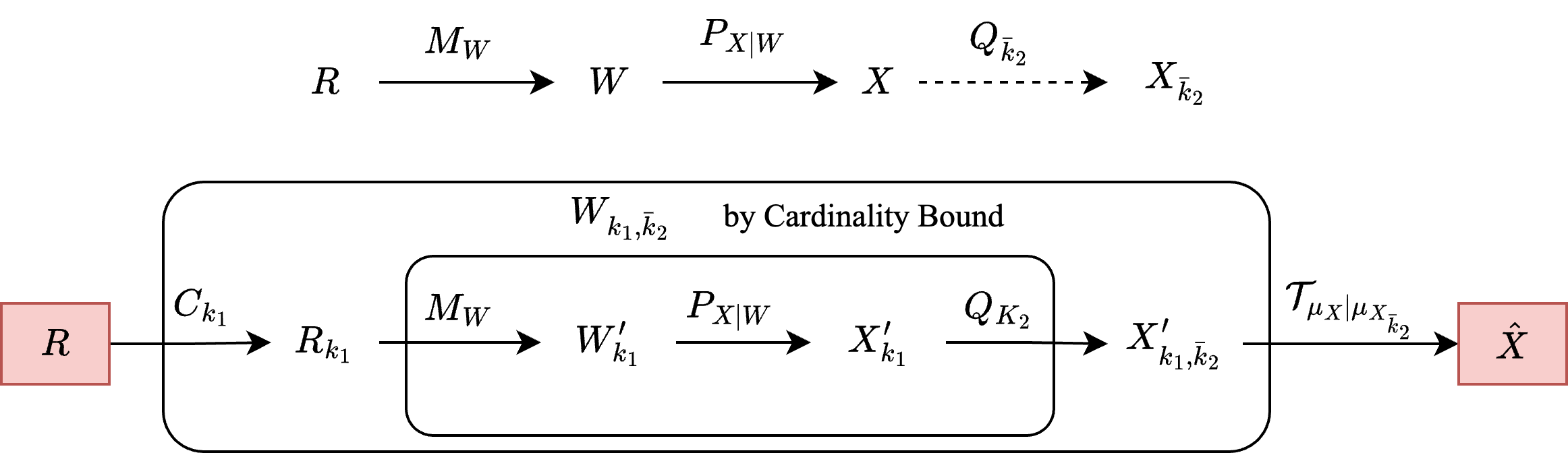
Figure 1: Markov Chain of the new Approach: The upper diagram shows the original Markov chain provided by the single-letter intermediate state $W$. The lower diagram shows the single-letter Markov chain of the new approach in which the clipped source state is directly fed into the same continuous measurement $M_{W}$ and the discrete output is obtained by quantizing $X^{\prime}_{k_{1}}$. Finally, the optimal transport transforms the discrete output back to the continuous output $\hat{X}$.

After applying the clipping measurement, the system has two possible scenarios which can be helpful in subsequent analysis. In the first scenario, the system reveals the outcome $A_{k_{1}}$, and based on its value, if the source state is inside the clipping subspace $(A_{k_{1}}=0)$, then $\hat{\rho}^{A^{\prime}}_{0}$ is sent to $M_{W}$ POVM to produce the classical outcome. Otherwise if $(A_{k_{1}}=1)$, we throw out the a-posteriori state $\hat{\rho}^{A^{\prime}}_{1}$ and only notify the receiver by asserting $A_{k_{1}}$. This scenario produces the following new Markov chain:

$$R\stackrel{{\scriptstyle C_{k_{1}}}}{{\longrightarrow}}R_{k_{1}}\stackrel{{\scriptstyle M_{W}}}{{\longrightarrow}}W^{\prime}_{k_{1}}\stackrel{{\scriptstyle P_{X|W}}}{{\longrightarrow}}X^{\prime}_{k_{1}}\stackrel{{\scriptstyle Q_{k_{2}}}}{{\longrightarrow}}X^{\prime}_{k_{1},\bar{k}_{2}}.$$ (76)

The second scenario is when the outcome $A_{k_{1}}$ is not revealed and thrown away. Then the system performs $M_{W}$ POVM on the post-projection state. Using (74), the final conditional a-posteriori average density operator for an event $B\in\mathcal{B}$ given the clipping POVM outcomes are

$$\hat{\rho}_{0}^{A^{\prime\prime}}(B)=\frac{\sqrt{M_{W}(B)}\rho_{A}\Pi_{k_{1}}\sqrt{M_{W}(B)}}{\Tr{M_{W}(B)\rho_{A}\Pi_{k_{1}}}},\quad\hat{\rho}_{1}^{A^{\prime\prime}}(B)=\frac{\sqrt{M_{W}(B)}\rho_{A}(I-\Pi_{k_{1}})\sqrt{M_{W}(B)}}{\Tr{M_{W}(B)\rho_{A}(I-\Pi_{k_{1}})}}.$$

Because $A_{k_{1}}$ is hidden, the average final a-posteriori density operator is

$$\hat{\rho}^{A^{\prime\prime}}(B)=\hat{\rho}_{0}^{A^{\prime\prime}}(B)\cdot\Pr{A_{k_{1}}=0|B}+\hat{\rho}_{1}^{A^{\prime\prime}}(B)\cdot\Pr{A_{k_{1}}=1|B}=\frac{\sqrt{M_{W}(B)}\rho^{A}\sqrt{M_{W}(B)}}{\Tr{M_{W}(B)\rho^{A}}}.$$ (77)

The above equality shows that by throwing out the outcome $A_{k_{1}}$, the system acts as if no clipping projection was performed, which reclaims the original Markov chain $R-W-X$.

Remark 6.

The importance of this second scenario is revealed in the next subsection while proving the rate inequalities. It is needed to establish a single probability space in which both unclipped outcome $W$ and $A_{k_{1}}$ exist. However, in reality, the continuous protocol only employs the first scenario.

As we had to define a separate Markov chain, we cannot directly harness the data processing inequality to prove the rate inequalities for the quantized and clipped systems. Therefore we provide the following proposition to show the rate inequalities still hold after clipping and quantization.

Proposition 2.

Suppose having a quantum Markov chain of the form $R-W-X$ satisfying the conditions in Theorem 2. Using the new clipping method as described by (76), the clipped states still satisfy the following rate inequalities in the asymptotic regime

$$\lim_{k_{1}\to\infty}I_{g}(R_{k_{1}};W^{\prime}_{k_{1}})\leq I_{g}(R;W),\quad\lim_{k_{1}\to\infty}I(W^{\prime}_{k_{1}};X^{\prime}_{k_{1},\bar{k}_{2}})\leq I(W;X).$$ (78)

Proof.

Proof in Appendix A.1 ∎

3.3.2 Source-Coding Protocol for Continuous States

Having a quantum source generating a sequence of $n$ independent continuous states $\rho^{\otimes n}$, we apply a coding protocol on the source states, described as follows. First, separate the input states into proper and improper states (the states residing inside and outside the clipping region respectively) by applying the clipping POVM $C_{k_{1}}$. This generates a sequence of error bits $A^{n}_{k_{1}}\equiv\{A_{i,k_{1}}\}_{i=1}^{n}$ where $A_{i,k_{1}}$ is the clipping error of the $i$-th state as defined in (73). Thus, according to Weak Law of Large Numbers, for any fixed $\epsilon_{cl}>0$ and $k_{1}\in\mathbb{N}$, there exists a value $N_{0}(\epsilon_{cl},k_{1})$ large enough such that for any $n\geq N_{0}(\epsilon_{cl},k_{1})$, the number of proper states

$$T:=\sum_{i=1}^{n}\left(1-A_{i,k_{1}}\right),$$ (79)

is within the range $T\in[n(1-P_{k_{1}}\pm\epsilon_{cl})]$ with probability no less than $1-\epsilon_{cl}$. Then for any sequence with $T<t_{\text{min}}$ where $t_{\text{min}}:=n(1-P_{k_{1}}-\epsilon_{cl})$, we do not perform source coding, and instead assert a source coding error event $E_{ce}$. Upon receiving the coding error event, Bob will locally generate a sequence of random outcomes $\hat{X}^{n}_{\text{local}}$ with the desired $\mu_{X}^{n}$ output distribution. This ensures that in every sequence for which the coding is performed, there are $T\geq t_{\text{min}}$ independent source states which are inside the clipping region, for which we apply the coding scheme. For the rest of the $(n-T)$ states, we do not perform the coding, instead, we throw away the source state and send the error-index to the receiver.

Next, the error bits sequence is coded into indices of size ${\binom{n}{t_{\text{min}}}}+1$ where the extra index is the event of a source coding error $E_{ce}$. Note here that the required classical rate, in this case, will be $R+\log_{2}\left({\binom{n}{t_{\text{min}}}}+1\right)$. The following limit

$$\lim_{\epsilon_{cl}\to 0}\lim_{k_{1}\to\infty}\lim_{n\to\infty}\frac{1}{n}\log_{2}\left({\binom{n}{n(1-P_{k_{1}}-\epsilon_{cl})}}+1\right)=0,$$ (80)

ensures that the extra error handling rate can be made arbitrarily small.

Then at Bob’s side, the classical sequence $X^{\prime t}_{k_{1},\bar{k}_{2}}$ is constructed using the discrete coding scheme, and is fed to a memoryless optimal transport block $\mathcal{T}_{\mu|\mu_{\bar{k}_{2}}}$ to generate the final continuous sequence $\hat{X}^{t}_{k_{1},\bar{k}_{2}}$. Finally, the sequence is padded with the $(n-T)$ locally generated independent values at the error positions to create the final $\hat{X}^{n}_{k_{1},\bar{k}_{2}}$. Bob then uses this sequence to prepare his final quantum states. Figure 2 shows the block diagram of this coding protocol.

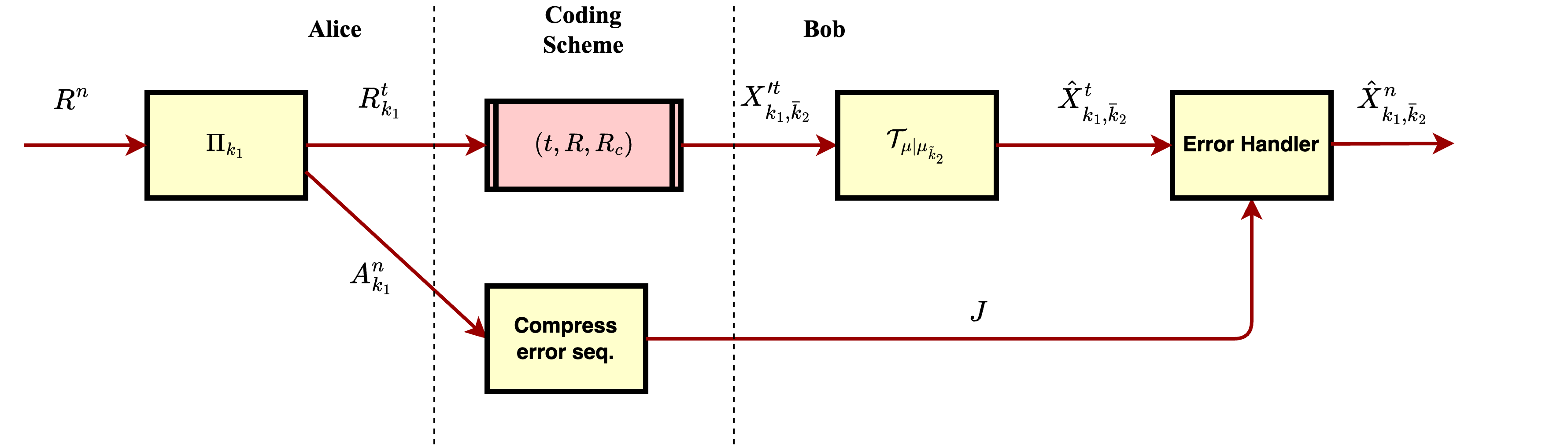
Figure 2: Continuous Coding Protocol

3.3.3 Proof of Distortion Constraint

The end-to-end average distortion for the above system is written as

$$d_{n}(R^{n},{\hat{X}}^{n}_{k_{1},\bar{k}_{2}}) =d_{n}\left(R^{n},{\hat{X}}^{n}_{k_{1},\bar{k}_{2}}\Big{|}E_{ce}\right)\Pr(E_{ce})+d_{n}\left(R^{n},{\hat{X}}^{n}_{k_{1},\bar{k}_{2}}\Big{|}\neg E_{ce}\right)\left(1-\Pr(E_{ce})\right)$$

$$\leq d_{n}\left(R^{n},\hat{X}_{\text{local}}^{n}|E_{ce}\right)\Pr(E_{ce})+d_{n}\left(R^{n},{\hat{X}}^{n}_{k_{1},\bar{k}_{2}}\Big{|}\neg E_{ce}\right)$$

$$=\frac{1}{n}\sum_{i=1}^{n}d\left(R_{i},\hat{X}_{i,\text{local}}|E_{ce}\right)\Pr(E_{ce})+d_{n}\left(R^{n},{\hat{X}}^{n}_{k_{1},\bar{k}_{2}}\Big{|}\neg E_{ce}\right),$$ (81)

where $\hat{X}_{\text{local}}^{n}$ is generated locally at Bob’s side according to the fixed IID output distribution $\mu_{X}$ in the event of coding error $E_{ce}$. Therefore, in the first term above, for each $i$-th sample of the system, the uniform integrability of the distortion observable implies that it can be made arbitrarily small by selecting the proper value of $\epsilon_{cl}$. As for the second term, we use the following lemma to provide a single-letter upper bound:

Lemma 1.

The end-to-end average n-letter distortion of the continuous system conditioned on the event of no coding error is bounded from above by the following single-letter distortion for any fixed value of $k_{1},k_{2},k_{2}^{\prime}>0$ and $\bar{\varepsilon}>0$ as:

$$d_{n}(R^{n},{\hat{X}}^{n}_{k_{1},\bar{k}_{2}}|\neg E_{ce}) \leq d(R_{k_{1}},X^{\prime}_{k_{1},\bar{k}_{2}})+\bar{\varepsilon}+\varepsilon(k_{1},k_{2}),$$ (82)

for all sufficiently large $n$. Furthermore, $\varepsilon\downarrow 0$ as $k_{1},k_{2}$ become large.

Proof.

See Appendix A.3 ∎

Next, note that the following inequality holds by definition for the single-letter discrete distortion:

$$d(R,X_{\bar{k}_{2}}) =d(R,X_{\bar{k}_{2}}|A_{k_{1}}=0)\Pr(A_{k_{1}}=0)+d(R,X_{\bar{k}_{2}}|A_{k_{1}}=1)\Pr(A_{k_{1}}=1)$$

$$=d(R_{k_{1}},X^{\prime}_{k_{1},\bar{k}_{2}})\Pr(A_{k_{1}}=0)+d(R,X_{\bar{k}_{2}}|A_{k_{1}}=1)\Pr(A_{k_{1}}=1).$$ (83)

Then, by having the probability of clipping approach zero $\lim_{k_{1}\to\infty}\Pr(A_{k_{1}}=1)=0$, the second term above goes to zero as a direct result of uniform integrability, and we have the following asymptotic limit:

$$\lim_{k_{1}\to\infty}d(R_{k_{1}},X^{\prime}_{k_{1},\bar{k}_{2}}) =d(R,X_{\bar{k}_{2}}):=\int_{\mathcal{X}}\Tr{\sqrt{\rho}\,\Lambda_{X}(dz)\sqrt{\rho}\,\Delta\big{(}Q_{\bar{k}_{2}}(z)\big{)}}.$$ (84)

Then as $k_{2},k_{2}^{\prime}\to\infty$, we can bound from above this RHS distortion value by

$$\lim_{k_{2},k^{\prime}_{2}\to\infty}d(R,X_{\bar{k}_{2}}) \leq D+\lim_{k_{2},k^{\prime}_{2}\to\infty}\left(d(R,X_{\bar{k}_{2}})-d(R,X)\right)$$

$$=D+\lim_{k_{2},k^{\prime}_{2}\to\infty}\int_{\mathcal{X}}\Tr{\sqrt{\rho}\,\Lambda_{X}(dz)\sqrt{\rho}\,\Big{(}\Delta\big{(}Q_{\bar{k}_{2}}(z)\big{)}-\Delta(z)\Big{)}}=D,$$ (85)

where the last equality follows similarly from continuity and uniform integrability of the distortion observable operator $\Delta(x)$ as a function of $x\in\mathcal{X}$. Combining the above bounds to the single-letter expression in (82) shows $\lim_{n\to\infty}d_{n}(R^{n},{\hat{X}}^{n}_{k_{1},\bar{k}_{2}})\leq D$, which completes the proof of achievability.

4 Evaluation of the Qubit-Binary System

In this section, we study the example of qubit-binary systems. Having the qubit source state $\rho$, a Bernoulli output distribution $Q_{X}$, and entanglement fidelity as the distortion measure, we aim to find the OC rate-distortion function $R(D;\infty,\rho||Q_{X})$ for the case of unlimited common randomness. By inverting this function we then achieve the RLOT cost $D(R;\infty,\rho||Q_{X})$ function. We then provide the numerical results for a few numerical examples and plot the rate-distortion function.

4.1 Qubit System with Unlimited Common Randomness

For the case of the qubit QC system, we employ entanglement fidelity [25, 26] as the distortion measure, which can be written as

$$\Tr{\Delta_{RX}\tau_{RX}}=1-\bra{\psi^{RA}}\left(\sum_{x}\sqrt{\rho}M_{x}\sqrt{\rho}\otimes\outerproduct{x}{x}\right)\ket{\psi^{RA}}.$$ (86)

Using the spectral decomposition of $\rho=\sum_{t=1,2}P_{T}(t)\outerproduct{\varphi_{t}}{\varphi_{t}}$, with the eigenbasis ${\ket{\varphi_{t}}}_{t=1}^{2}$, and by substituting the canonical purification of the above decomposition into (86), it simplifies to

$$\Tr{\Delta_{RX}\tau_{RX}} =1-\sum_{x}\bra{x}\rho M_{x}^{\mathcal{T}_{\varphi}}\rho\ket{x},$$ (87)

where $M_{x}^{\mathcal{T}_{\varphi}}$ is the transpose of $M_{x}$ with respect to the $\{\varphi_{t}\}$ basis, defined as

$$M_{x}^{\mathcal{T}_{\varphi}}=\sum_{t,s}\innerproduct{\varphi_{t}}{M_{x}|\varphi_{s}}\outerproduct{\varphi_{t}}{\varphi_{s}}.$$ (88)

Remark 7.

Although the distortion formula in (87) has transposed POVM operator $M_{0}^{\mathcal{T}_{\varphi}}$, we can ignore this transpose in the distortion constraint of the above optimization problem. The reason is that the eigenvalues of $\rho_{x}$ are preserved under the transposition with respect to any basis. This implies that the entropy function also does not change under transposition.

In the presence of an unlimited amount of common randomness, the only effective rate becomes $I(W;R)$, which is lower-bounded by $I(X;R)$ because of the data processing inequality and the Markov chain $R-W-X$ [12]. Thus $W=X$ minimizes the mutual information, which means no local randomness is required at the decoder. Therefore, using the main theorem, for a qubit system with input state $\rho$ and Bernoulli($q_{1}$) output distribution, the OC rate-distortion function is obtained by

$$R(D;\infty,\rho||\text{Bern}(q_{1}))= \min_{M_{x}^{A}}I(R;X)_{\tau},=\min_{M_{x}^{A}}\left[H(\rho)-\Big{(}q_{0}H(\hat{\rho}_{0})+q_{1}H(\hat{\rho}_{1})\Big{)}\right]$$ (89)

subject to: $$\begin{array}[]{l}\Tr{M_{x}\rho}=q_{x},\quad\quad x=0,1,\\ \sum_{x}\Tr_{A}\left\{(\text{id}_{R}\otimes M_{x})\psi^{RA}\right\}=\rho,\\ 1-\sum_{x}\bra{x}\rho M_{x}^{\mathcal{T}_{\varphi}}\rho\ket{x}\leq D.\end{array}$$ (93)

where the information quantity is with respect to the composite state $\tau_{RX}=\sum_{x}\hat{\rho}_{x}\otimes\outerproduct{x}{x}^{X}.$

4.1.1 Rate-Limited Optimal Transport for Qubit Measurement System

By addressing the above optimization problem, we obtain Theorem 3, which yields a transcendental system of equations that determines the OC rate-distortion function for this system. We first define the quantum source $\rho$ and some operator, $N(n,s)$ in the following matrix format:

$$\rho=\begin{bmatrix}\rho_{1}&\rho_{2}\\ \rho_{2}^{*}&1-\rho_{1}\end{bmatrix},\quad N(n,s):=\begin{bmatrix}n&s\rho_{2}/|\rho_{2}|\\ s\rho_{2}^{*}/|\rho_{2}|&q_{0}-n\end{bmatrix},$$ (94)

for some $\rho_{1},\rho_{2},n$, and $s$, where $n$ and $s$ depend on the measurement operator $M_{0}$ and need to be determined by solving the optimization problems. We also define the following parameters:

$$E_{1}(n,s) :=\sqrt{\left(n-\frac{q_{0}}{2}\right)^{2}+s^{2}},\qquad\qquad\qquad\qquad E_{2}(n,s):=\sqrt{\left(n-\rho_{1}+\frac{1-q_{0}}{2}\right)^{2}+(s-|\rho_{2}|)^{2}},$$ (95)

$$a :=1-\frac{4|\rho_{2}|^{2}}{1+2k},\qquad\qquad\qquad\qquad\qquad\qquad\qquad b:=\frac{2|\rho_{2}|(2\rho_{1}-1)}{1+2k},$$ (96)

$$c :=q_{0}\left(\rho_{1}-1+\frac{2|\rho_{2}|^{2}}{1+2k}\right)+\innerproduct{1|\rho^{2}}{1}-1+D,\ \ k:=\sqrt{\det{\rho}}.$$ (97)

For the qubit measurement system, let $D_{OT}:=D(R=\infty,R_{c},\rho||\text{Bern}(q_{1}))$ denote the QC optimal transportation cost, which is characterized in Theorem 4 in the next subsection. With these definitions of the parameters in place, we can characterize the OC rate-distortion function as follows.

Theorem 3.

For the case of qubit input state $\rho$ the OC rate-distortion function and the corresponding optimal POVMs $M_{0},M_{1}$ are provided as follows:

$$R(D;\infty,\rho||\text{Bern}(q_{1})) =\begin{cases}H(\rho)-q_{0}H\left(N_{opt}/q_{0}\right)-(1-q_{0})H\left((\rho-N_{opt})/q_{1}\right),&D_{OT}\leq D\leq D_{R_{0}},\\ 0,&D_{R_{0}}\leq D\end{cases}$$ (98)

where $D_{R_{0}}:=1-q_{0}\innerproduct{0}{\rho^{2}|0}-(1-q_{0})\innerproduct{1}{\rho^{2}|1}$. In the first case, POVM elements are $M_{0}=q_{0}I$, and $M_{1}=q_{1}I$. In the second case, they are $M_{0}=\sqrt{\rho}^{-1}N_{opt}\sqrt{\rho}^{-1},\quad M_{1}=I-M_{0}$. Also, $N_{opt}/q_{0}=N(n,s)/q_{0}$ with the optimal $n,s$ values, is the optimal PMR state conditioned on outcome zero, and that optimal $n,s$ satisfy the transcendental system of equations:

$$\begin{cases}\frac{-as+b(n-q_{0}/2)}{E_{1}}\ln{\frac{q_{0}/2+E_{1}}{q_{0}/2-E_{1}}}+\frac{-a(s-|\rho_{2}|)+b(n-\rho_{1}+\frac{1-q_{0}}{2})}{E_{2}}\ln{\frac{\frac{1-q_{0}}{2}+E_{2}}{\frac{1-q_{0}}{2}-E_{2}}}&=0.\\ an+bs+c&=0.\end{cases}$$ (99)

Proof.

See Appendix B. ∎

Remark 8.

The following two special source states result in interesting $N_{opt}$ optimal matrices. (I) Pure input state: For the case of pure input state, the rate-distortion curve reduces to a single point where the rate is $R=0$, the optimal $N_{opt}=q_{0}\rho$ and $D=D_{R_{0}}$. This is because the pure input state has no correlation with the reference, so the receiver can simply use local randomness in its decoder. (II) Diagonal (among canonical eigen-basis) quantum input state: In this case, the optimal operator $N_{opt}$ will also be diagonal.

4.1.2 Optimal Transport for Qubit Measurement System

The optimal transport scheme provides the minimum achievable distortion when the rate of information is not limited. The following theorem provides this value for the problem of the qubit measurement system.

Theorem 4.

Defining the parameter $Q:=\frac{\rho_{1}-1/2}{\sqrt{1-4|\rho_{2}|^{2}}}$, the optimal transportation cost $D_{OT}$ is given by:

$$D_{OT} =\begin{cases}q_{0}(1-\rho_{1})+\det(\rho)+\frac{1-q_{0}}{2}\left(1-\sqrt{1-4|\rho_{2}|^{2}}\right),&\text{if }\quad Q\leq\frac{\det(\rho)}{1-q_{0}}-\frac{1}{2}\\ (1-q_{0})\rho_{1}+\det(\rho)+\frac{q_{0}}{2}\left(1-\sqrt{1-4|\rho_{2}|^{2}}\right),&\textbf{ if }\quad Q\geq\frac{1}{2}-\frac{\det(\rho)}{q_{0}}\\ 1-q_{0}\left(\rho_{1}-1+\frac{2|\rho_{2}|^{2}}{1+2k}\right)-\innerproduct{1|\rho^{2}}{1}-a\alpha-b\beta,&\text{ if }\quad\frac{\det(\rho)}{1-q_{0}}-\frac{1}{2}\leq Q\leq\frac{1}{2}-\frac{\det(\rho)}{q_{0}}\end{cases}$$ (100)

where $\alpha$ and $\beta$ are the parameters given below and $\Delta^{\prime}:=\left(q_{0}(1-q_{0})-\det(\rho)\right)\det(\rho)$,

$$\alpha =\frac{\left(q_{0}-2\det(\rho)\right)|\rho_{2}|+\text{sgn}\{a-b\}(1-2\rho_{1})\sqrt{\Delta^{\prime}}}{4|\rho_{2}|^{2}+(1-2\rho_{1})^{2}},$$

$$\beta =\frac{2q_{0}|\rho_{2}|^{2}-(1-2\rho_{1})(\rho_{1}q_{0}-\det(\rho))+\text{sgn}\{a-b\}2|\rho_{2}|\sqrt{\Delta^{\prime}}}{4|\rho_{2}|^{2}+(1-2\rho_{1})^{2}}.$$

Proof.

See Appendix C. ∎

Interestingly, when the input state is prepared with the diagonal density operator along the eigenbasis of the output state (i.e. $\rho_{2}=0$), the optimal matrices $N_{opt}$ and $\rho-N_{opt}$ encompasses the classical binary optimal transport scheme. One can see that the first and second conditions reduce to $q_{0}\geq\rho_{1}$ and $q_{0}<\rho_{1}$ and the third condition is empty. However, the distortion value will be obviously different.

4.2 Numerical Results

We used the CVX package [66, 67] to find numerical solutions for the examples of this convex optimization problem. Also [68] provides the CVX functions for the von-Neumann entropy functions. The OC rate-distortion function is numerically evaluated for the following set of examples (a), (b), (c) and (d) with fixed $q_{0}=1/2$ and $\rho_{1}=1/2$ parameters and different off-diagonal values:

$$\text{Ex1: }\rho_{a}=\begin{bmatrix}1/2&0\\ 0&1/2\end{bmatrix}, \text{Ex2: }\rho_{b}=\begin{bmatrix}1/2&0.132-0.036i\\ 0.132+0.036i&1/2\end{bmatrix},$$

$$\text{Ex3: }\rho_{c}=\begin{bmatrix}1/2&0.075-0.231i\\ 0.075+0.231i&1/2\end{bmatrix}, \text{Ex4: }\rho_{d}=\begin{bmatrix}1/2&-0.140-0.387i\\ -0.140+0.387i&1/2\end{bmatrix},$$

with the purity values $\Tr{\rho_{a}^{2}}=0.500$, $\Tr{\rho_{b}^{2}}=0.537$, $\Tr{\rho_{c}^{2}}=0.618$ and $\Tr{\rho_{d}^{2}}=0.839$. These rate-distortion functions are plotted in Figure 3, which shows that starting from a maximally mixed state (Ex.1.), as the source state becomes purer, it requires less communication rate to maintain the same level of entanglement fidelity.

In the case of a pure source state, the rate-distortion function reduces to a single point at the no transmission rate. This is intuitively acceptable as the pure state is independent of the reference state. So the receiver can generate random outcomes independent of the source. However, the entanglement fidelity distortion will not be zero because the measurement collapses the state into deterministic outcomes and hence it will not fully recover the source state. On the contrary, the maximally mixed state has the maximum dependence on the reference state which requires the maximum rate of transmission to recover the state with the same level of distortion.

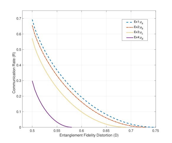
Figure 3: The OC rate-distortion function with unlimited common randomness for the examples

5 Evaluation of the Gaussian Quantum States

5.1 A Brief Overview of Gaussian Quantum Systems

Before providing the evaluation of the Gaussian systems, we first introduce the principal definitions and provide a brief overview of the Gaussian quantum systems.

5.1.1 Gaussian Quantum Systems

Let $\mathcal{H}_{A}\equiv\mathcal{L}^{2}(\mathbb{R}^{s})$ be the separable infinite-dimensional Hilbert space of the square-integrable functions $\psi(\eta)$ for $\eta\in\mathbb{R}^{s}$ corresponding to $s$ Harmonic oscillators. The canonical observable operators of this system are $Q_{1}$, $P_{1}$, $Q_{2}$, $P_{2},...,Q_{s}$, $P_{s}$ with continuous eigenspectra, where $Q_{i},P_{i}$ are the position and momentum quadrature operators of the $i$-th harmonic oscillator. In this section, we consider the energy-bounded harmonic oscillator system as described by [22, 38]. Then referring to Lemma 11.5 of Holevo’s [38], we note that a subset of energy-bounded states $\mathcal{G}_{E}\subset\mathcal{G}(\mathcal{H})$ with a corresponding energy operator $F$ defined as $\mathcal{G}_{E}:=\{S:\Tr{SF}\leq E\}$, is compact. The canonical observables satisfy the Canonical Commutation Relation (CCR) resulting from the Heisenberg uncertainty principle. For more convenience, we combine the quadrature operators as elements of a $2s\times 2s$ vector operator, $R_{1}=Q_{1},\;R_{2}=P_{1},\;\cdots,\;R_{2s-1}=Q_{m},\;R_{2s}=P_{s},$ which redefines the CCR as $[R_{i},R_{j}]=i\Delta_{ij}I_{\mathcal{H}},$ for $i,j=1,...,2m,$ with $\Delta$ being a non-degenerate skew-symmetric symplectic matrix defined as $\Delta=\bigoplus_{k=1}^{s}\begin{bmatrix}0&1\\ -1&0\end{bmatrix}.$

The Weyl operator is further defined by $W(z)=\exp{iRz}$ where $z:=[q_{1},p_{1},...,q_{s},p_{s}],z\in\mathbb{R}^{2s}$ is a vector of values in some phase space corresponding to the eigenvalues of the quadrature operators. The displacement operator is also defined by $D(m):=W(\Delta^{-1}m)$. The Wigner characteristic function is further given by $\phi_{\rho}(z)=\Tr{\rho W(z)}$. The domain of the Wigner function $\mathcal{Z}=\mathbb{R}^{2s}$ together with the symplectic matrix $\Delta$ form a symplectic space $\mathcal{K}:=(\mathcal{Z},\Delta)$ which is called the phase space.

For a density operator $\rho$, the mean vector and covariance matrix are given by $m=\Tr{\rho R}$, and $\alpha-\frac{i}{2}\Delta=\Tr{(R-m)^{T}\rho\ (R-m)}$, respectively, where $\alpha$ is the covariance matrix of the Wigner quasi-probability distribution. Further, the following inequality holds (in the positive semi-definite sense) for the covariance matrix of the quantum state which is a result of the uncertainty principle:

$$\alpha\geq\pm\frac{i}{2}\Delta.$$ (101)

The eigenvalues of $\alpha$ depended on the, and have no significance. However, for the operator $\tilde{\alpha}=\absolutevalue{\Delta^{-1}\alpha}$, the eigenvalues $\pm i\gamma_{j}$, for $j=1,\cdots,s$ are called the symplectic eigenvalues. The uncertainty relation (101) translates to $\alpha_{j}>1/2$ or described as $\left(\Delta^{-1}\alpha\right)^{2}\geq-\frac{1}{4}I$, with equality when the system is in a pure state [36]. In the special case when the state is a product state of the modes, which is when $\alpha$ is a block-diagonal of $s$ separate 2-by-2 matrices, the symplectic eigenvalues are simply the determinant of each mode $\gamma_{j}=\det{\alpha_{j}}$ [35]. The quantum Gaussian state is defined on $\mathcal{H}$ as a state whose Wigner characteristic function and the Wigner quasi-probability function are Gaussian and given by:

$$\phi_{\rho}(z) =\exp[-\frac{1}{2}z^{T}\alpha z+im^{T}z],\quad\Phi_{\rho}(x)=\frac{\exp[-\frac{1}{2}(z-m)^{T}\alpha^{-1}(z-m)]}{(2\pi)^{s}\sqrt{\det\alpha}}.$$

Similar to classical Gaussian distributions, for a Gaussian quantum state, the displacement and covariance matrix are sufficient to fully represent the Gaussian state. For a more detailed review of the Gaussian quantum systems see [38, 69, 70, 39].

5.1.2 Gaussian Observables

The measurement POVM $M$ has a general form as defined in [38]. For any observable POVM $M$ with the PMR ensemble $\{\rho_{z},\pi_{Z}(dz)\}_{z\in\mathcal{Z}}$, the information gain function is defined as

$$I_{g}(\rho_{N};M)=H(\rho_{N})-\int_{\mathcal{Z}}H(\rho_{z})\pi_{Z}(dz).$$ (102)

An important group of observables is the general form of the covariant Gaussian observable as provided in [37]:

$$\tilde{M}(d^{2s}z)=D(Kz)\rho_{G}D(Kz)^{\dagger}\frac{\absolutevalue{\det K}^{2}d^{2s}z}{\pi^{s}},$$ (103)

where $\rho_{G}$ is a density operator that is the parameter of the Gaussian observable and is different from the input density operator $\rho_{N}$. The von-Neumann entropy of the general Gaussian state with covariance matrix $\alpha$ is given by [36],

$$H(\rho_{N})=H_{G}(\alpha):=\frac{1}{2}\text{Sp}g\left(\absolutevalue{\Delta^{-1}\alpha}-\frac{I}{2}\right).$$ (104)

where $\mathrm{Sp}\left(.\right)$ is the matrix trace as opposed to the $\Tr(.)$ the trace in Hilbert space and that $g(x)=(x+1)\log(x+1)-x\log x$, for $x>0$, and $g(0)=0$ is the Gordon function.

5.1.3 Distortion Observable

To introduce the distortion observable, we first provide the following definitions. Let $\mathcal{H}^{*}$ be the space of continuous linear functionals on Hilbert space $\mathcal{H}$ [22]. We consider the following definition of the transposition.

Definition 5.1.

For any operator $X\in\mathcal{L}(\mathcal{H})$, let $X^{T}$ be the linear operator on $\mathcal{H}^{*}$ given by

$$X^{T}\bra{\phi}=\bra{\phi}X\quad\text{for all }\bra{\phi}\in\mathcal{H}^{*}.$$ (105)

For finite-dimensional Hilbert spaces, this reduces to the definition of transpose specified in (88).

Remark 9.

Assume having a source state $\rho\in\mathcal{H}_{A}$ and a measurement POVM with outcomes $z\in\mathcal{Z}$. Then the conditional PMR states $(\hat{\rho}_{z}^{\mathcal{T}})^{R}$ and the unrevealed PMR state $(\rho^{\mathcal{T}})^{R}$ live in $\mathcal{H}^{*}$ [29, 22]. Furthermore, as was mentioned in remark 7, the entropic quantities are invariant under the transposition.

The following distortion observable operator was introduced by [22] using the quadrature operators,

$$C=\frac{1}{2s}\sum_{i=1}^{2s}(R_{i}^{\mathcal{T}}\otimes I_{\mathcal{H}}-I_{\mathcal{H}^{*}}\otimes R_{i})^{2}.$$ (106)

This operator was defined to address the problem of quantum optimal transport for Gaussian quantum states. The significance of the operator is that it acts on the composite state of the reference and the destination system in the $\mathcal{H}^{*}\otimes\mathcal{H}$ space. As a result, the optimal coupling that minimizes this distortion measure has a unique correspondence to the physical quantum channels. Note that, in a fully quantum setting, applying this observable to a purified state $\Psi^{RA}$ yields zero distortion, i.e., $\Tr{\Psi^{RA}C}$=0, because the observations on the local state and on the reference state have equal values with probability $1$. The transpose operation is essential because the reference state resides in the $\mathcal{H}^{*}$ Hilbert space, therefore, if we want to compare the outcomes of the states, we must use the $R_{i}^{\mathcal{T}}$ operator for the reference so that $\Tr{R^{\mathcal{T}}\rho^{\mathcal{T}}}=\Tr{R\rho}$. For a more detailed explanation refer to [70, 22].

We use this distortion observable that acts on $\mathcal{H}^{*}\otimes\mathcal{H}$ and modify it in a way that fits our QC Gaussian measurement system. Consider a POVM $\Lambda$ with outcomes in $\mathcal{Z}$. Let $\pi_{Z}(B)=\Tr{\rho^{A}\Lambda(B)}$ for all $B\in\mathcal{B}(\mathcal{Z})$. We define the distortion of the PMR ensemble $\{\{\hat{\rho}_{z}\}_{z\in\mathcal{Z}},\pi_{Z}\}$, in a similar fashion to the distortion observable mapping $x\mapsto\Delta_{R}(x)$, described in Subsection 2.1.1 as

$$d(\rho_{A},\Lambda) :=\frac{1}{2s}\sum_{i=1}^{2s}\int_{\mathcal{Z}}\Bigl{[}\Tr{\hat{\rho}_{z}^{R}(R_{i}-\bar{m}_{i}(z))^{2}}+\innerproduct{z|(R_{i}-\bar{m}_{i}(z))^{2}}{z}\Bigr{]}\pi_{Z}(dz)$$ (107)

$$=\frac{1}{2s}\sum_{i=1}^{2s}\int_{\mathcal{Z}}\Bigl{[}\left\{\Sigma(z)\right\}_{ii}+(z_{i}-\bar{m}_{i}(x))^{2}\Bigr{]}\pi_{Z}(dz)$$ (108)

$$=\frac{1}{2s}\int_{\mathcal{Z}}\left(\text{Sp}\{\Sigma(z)\}+{\norm{z-\bar{m}(z)}_{2}^{2}}\right)\pi_{Z}(dz):=d(\rho_{Z},\pi_{Z}),$$ (109)

where $\bar{m}_{i}(z)=\Tr{\hat{\rho}^{R}_{z}R_{i}}=\Tr{{(\hat{\rho}_{z}^{\mathcal{T}})}^{R}R^{\mathcal{T}}_{i}}$ is the first moment and $\Sigma(z)$ is the covariance matrix of the state $\hat{\rho}^{R}_{z}$. Further, note that a Gaussian measurement system with the above distortion measure, satisfies the uniform integrability property defined in 3.4. For the proof see Appendix A.4.

5.2 Problem Formulation

In this subsection, we formulate the QC optimal transport for the case of Gaussian quantum systems with Gaussian source states and Gaussian output distribution. Recall the single-letter conditions of the rate pair in Theorem 2. We further restrict our evaluation to the systems with unlimited common randomness $(R_{c}=\infty)$. In that case, we can restrict ourselves to $W=Z$ as in Section 4. Moreover, due to the ensemble-observable duality [37], instead of searching for the optimal measurement itself, we can search for the optimum measurement outcome ensembles $\{\{\hat{\rho}_{z}\}_{z\in\mathcal{Z}},\pi_{Z}\}$. In that case, the OC rate-distortion function is defined by the following optimization problem:

$$R(D;R_{c}=\infty,\rho||\pi_{Z}):= \min_{\{\hat{\rho}_{z}:\ z\in\mathcal{Z}\}}\left[H(\rho)-\int_{\mathcal{Z}}H(\hat{\rho}_{z})\pi_{Z}(dz)\right]$$ (110)

subject to: $$\int_{\mathcal{Z}}\hat{\rho}_{z}\pi_{Z}(dz)=\rho,$$ (111)

$$\frac{1}{2s}\int_{\mathcal{Z}}\left(\mathrm{Sp}\{\Sigma(z)\}+{\norm{z-\bar{m}(z)}_{2}^{2}}\right)\pi_{Z}(dz)\leq D.$$ (112)

Definition 5.2.

The rate-limited Wasserstein distance $W_{2}(R,\rho||\pi_{Z})$ of the system is defined as the square root of the inverse of the above OC rate-distortion function within the proper range. The QC Wasserstein distance of order 2 is defined by $W_{2}(\rho||\pi_{Z}):=W_{2}(\infty,\rho||\pi_{Z})$. Then the rate of QC Wasserstein distance is defined as the lowest rate achieving the Wasserstein distance:

$$R_{W_{2}}(\rho||\pi_{Z}):=\inf\Big{\{}R:W_{2}(R,\rho||\pi_{Z})=W_{2}(\rho||\pi_{Z})\Big{\}}.$$ (113)

5.3 Main Result: Optimality of Gaussian Quantum Measurement

We provide a Gaussian measurement optimality theorem which shows that for the aforementioned OC rate-distortion quantum measurement system, with Gaussian source state and Gaussian output distribution and unlimited common randomness, the Gaussian observables achieve the optimal rate. We first provide the following lemma which is the QC version of the law of total variance. Consider a measurement that is applied on a source state $\rho$ and results in the PMR ensemble $\{\{\hat{\rho}_{z}^{\mathcal{T}}\}_{z\in\mathcal{Z}},\pi_{Z}\}$. In this setting, $\bar{m}(Z)=\Tr{\hat{\rho}_{Z}R}$ can be interpreted as the classical estimator of the source state $\rho$. The following lemma provides the relation for the covariance matrix of this estimator.

Lemma 2.

(QC Law of Total Variance) For a source quantum state $\rho$ with first moment $\bar{m}_{\rho}$ and covariance $\Sigma_{\rho}$ and a measurement POVM with the corresponding PMR ensemble $\{\{\hat{\rho}_{z}^{\mathcal{T}}\}_{z\in\mathcal{Z}},\pi_{Z}\}$, we have,

$$\Sigma_{\rho}=\int\hat{\Sigma}(z)\pi_{Z}(dz)+\tilde{\Sigma},$$ (114)

where,

$$\Sigma_{\rho}-\frac{i}{2}\Delta= \Tr{\rho(R-\bar{m}_{\rho})(R-\bar{m}_{\rho})^{T}}$$ (115)

$$\hat{\Sigma}(z)-\frac{i}{2}\Delta= \Tr{\hat{\rho}_{z}(R-\bar{m}(z))(R-\bar{m}(z))^{T}}\quad\text{for all }z\in\mathcal{Z}$$ (116)

$$\tilde{\Sigma}:= \text{Cov}(\bar{m}(Z))=\mathbb{E}_{Z}\left[{\bar{m}(Z)\bar{m}(Z)^{T}}\right]-\bar{m}_{\rho}\bar{m}_{\rho}^{T}$$ (117)

are the covariance matrix of the source, the conditional covariance of PMR state $\hat{\rho}_{z}$ and the covariance of the classical estimator $\bar{m}(Z)$ respectively.

Proof.

Starting with the second moment of the source state

$$\Tr{\rho RR^{T}} =\Tr{\left(\int\hat{\rho}_{z}\pi_{Z}(dz)\right)RR^{T}}=\int\left(\hat{\Sigma}(z)-\frac{i}{2}\Delta+\bar{m}(z)\bar{m}(z)^{T}\right)\pi_{Z}(dz),$$ (118)

then the covariance of the source state is

$$\Sigma_{\rho} =\Tr{\rho RR^{T}}-\bar{m}_{\rho}\bar{m}_{\rho}^{T}+\frac{i}{2}\Delta=\int\left(\hat{\Sigma}(z)\right)\pi_{Z}(dz)+\mathbb{E}_{Z}\left[{\bar{m}(z)\bar{m}(z)^{T}}\right]-\bar{m}_{\rho}\bar{m}_{\rho}^{T}.$$ (119)

∎

Using the above lemma we provide the following Gaussian optimality theorem.

Theorem 5.

In a quantum measurement system, suppose having a Gaussian quantum source state $\rho\sim\mathcal{QN}(\bar{m}_{\rho},\Sigma_{\rho})$ and a classical Gaussian output distribution $\pi_{Z}\equiv\mathcal{N}(\mu_{Z},\Sigma_{Z})$. Also, suppose using the quadratic distortion observable operator (106) as the distortion measure. Then, for any feasible distortion value $D$, the information gain $I_{g}(R;Z)$ is minimized by a Gaussian observable. This optimal Gaussian observable has the output ensemble representation $\{\tilde{\rho}_{N_{G},z},\pi_{Z}(dz)\}_{z\in\mathcal{Z}}$ with post-measured states

$$\tilde{\rho}_{N_{G},z}:=D(Kz)\rho_{N_{G}}D(Kz)^{\dagger}$$ (120)

where $\rho_{N_{G}}\sim\mathcal{QN}(0,\Sigma_{N})$ is a zero-mean Gaussian state representing the measurement noise with some $\Sigma_{N}$ such that $\Sigma_{N}\leq\Sigma_{\rho}$ to be determined and $K$ is a transformation matrix of the form

$$K=\Sigma_{Z}^{-1/2}\left(\Sigma_{Z}^{1/2}(\Sigma_{\rho}-\Sigma_{N})\Sigma_{Z}^{1/2}\right)^{1/2}\Sigma_{Z}^{-1/2}.$$ (121)

Proof.

With no loss of generality, we first assume that the quantum source state and the classical output distribution are both transported to the origin having zero means. Assume having an arbitrary set of PMR states $\{\hat{\rho}_{z}\}_{z\in\mathcal{Z}}$ with mean values $\bar{m}(z)$ and covariance matrices $\hat{\Sigma}(z)$. According to lemma 2, the following relation holds for the covariances:

$$\Sigma_{\rho}=\int\hat{\Sigma}(z)\pi_{Z}(dz)+\tilde{\Sigma}.$$ (122)

We further define a centralized version of the PMR states

$$\hat{\rho}_{c,z}:=D^{\dagger}(\bar{m}(z))\ \hat{\rho}_{z}\ D(\bar{m}(z)).$$ (123)

Thus, we have the following upper bound for the conditional entropy of PMR states

$$H(R|Z)=\int H\left(\hat{\rho}_{c,z}\right)\pi_{Z}(dz)\leq H\left(\hat{\rho}_{N}:=\int\hat{\rho}_{c,z}\ \pi_{Z}(dz)\right)\leq H(\tilde{\rho}_{N_{G}}),$$ (124)

where the first inequality follows from the concavity of von Neumann entropy [33, Property 11.4.1]. We defined $\hat{\rho}_{N}$ to be the average state with zero mean and the covariance matrix $\Sigma_{N}$, where

$$\Sigma_{N} =\Tr{\hat{\rho}_{N}RR^{T}}=\Tr{\left(\int D^{\dagger}(\bar{m}(z))\ \hat{\rho}_{z}\ D(\bar{m}(z))\pi_{Z}(dz)\right)RR^{T}}=\int\hat{\Sigma}(z)\pi_{Z}(dz).$$ (125)

Then by comparing (125) with (122) we find the covariance of the classical estimator, $\tilde{\Sigma}=\Sigma_{\rho}-\Sigma_{N}$.

Also in (124), in the last inequality, $\tilde{\rho}_{N_{G}}$ is introduced as a zero-mean Gaussian quantum state with the same covariance matrix $\Sigma_{N}$ which appeals to the quantum Gaussian entropy maximization theorem [35, Property (i)]. Further, the distortion function for the arbitrary PMR ensemble is

$$d(\hat{\rho}_{z},\pi_{Z})=\frac{1}{2s}\ \int\left[\mathrm{Sp}\left(\hat{\Sigma}(z)\right)+\norm{z-\bar{m}(z)}_{2}^{2}\right]\pi_{Z}(dz)=\frac{1}{2s}\ \mathrm{Sp}\left(\Sigma_{N}\right)+\frac{1}{2s}\int\norm{z-\bar{m}(z)}_{2}^{2}\pi_{Z}(dz).$$ (126)

We next form a different set of PMR ensembles equivalent to the quantum Gaussian measurement of the form $\tilde{\rho}_{z}=D(Kz)\tilde{\rho}_{N_{G}}D(Kz)^{\dagger}$, with $K$ being some transformation matrix to be determined.

Note that by using $\tilde{\rho}_{z}$, because the covariance matrix $\Sigma_{N}$ is fixed, the first term of the distortion (126) does not change. We further limit the selection of the $K$ matrix such that it satisfies the relation $\tilde{\Sigma}=K\Sigma_{Z}K^{T}$ with the covariance matrix of the estimator. This, again using lemma 2, makes sure that the marginal constraint is satisfied $\rho=\int\tilde{\rho}_{z}\pi_{Z}(dz)$ because the source quantum state is assumed to be Gaussian and can be fully determined by its first moment and covariance matrix [22]. The second term of distortion (126) is only a function of $\bar{m}(z)$.

So by preserving the covariance matrix $\tilde{\Sigma}=\Sigma_{\rho}-\Sigma_{N}$, we can provide the following lower bound

$$\mathbb{E}_{Z}\left[{\norm{\bar{m}(Z)-Z}_{2}^{2}}\right]\geq W_{2}^{2}\left(\mathcal{N}(\Sigma_{\rho}-\Sigma_{N})\;,\;\mathcal{N}(\Sigma_{Z})\right)=\mathbb{E}_{Z}\left[{\norm{Z-KZ}_{2}^{2}}\right].$$ (127)

where the inequality appeals to the following arguments. The $l_{2}$ norm depends only on the first two moments of the distributions, hence, one can replace them to Gaussian distributions. The lower bound on this distance is then the Wasserstein distance between these Gaussian distributions. Then the last equality follows by choosing $K$ to be the transportation that achieves the minimum distance from Gaussian distribution with $\Sigma_{Z}$ to Gaussian distribution with $\tilde{\Sigma}$ [71], i.e.,

$$K:=\Sigma_{Z}^{-1/2}\left(\Sigma_{Z}^{1/2}(\Sigma_{\rho}-\Sigma_{N})\Sigma_{Z}^{1/2}\right)^{1/2}\Sigma_{Z}^{-1/2}.$$ (128)

Then the following lower bound holds for the distortion

$$d(\hat{\rho}_{z},\pi_{Z})\geq\frac{1}{2s}\mathrm{Sp}\left(\Sigma_{N}\right)+\mathbb{E}_{Z}\left[{\norm{Z-KZ}_{2}^{2}}\right].$$ (129)

This shows that for a fixed noise covariance $\Sigma_{N}$, the PMR ensemble of the Gaussian form $\tilde{\rho}_{z}$ with $\bar{m}(z)=Kz$, does not decrease the conditional entropy while also preserving the distortion and marginal constraints. This proves that the Gaussian observable achieves the optimality. ∎

Corollary 6.

The following rate and distortion are achievable:

$$I_{g}(R;X) =H_{G}(\Sigma_{\rho})-H_{G}(\Sigma_{N}),$$ (130)

$$d(\tilde{\rho}_{N_{G},z},\pi_{Z}) =\frac{1}{2s}\left(\mathrm{Sp}\left(\Sigma_{N}\right)+\mathbb{E}_{\bar{\pi}_{Z}}\left[{Z-KZ}\right]+\norm{\bar{m}_{\rho}-\mu_{Z}}_{2}^{2}\right),$$ (131)

where the expectation in the second term is with respect to $\bar{\pi}_{Z}(B)=\pi_{Z}(B-\mu_{Z})$ for $B\in\mathcal{B}(\mathcal{Z})$.

5.4 The QC Gaussian Optimal Transport

To obtain the OC rate-distortion function, by using the above Gaussian optimality theorem, it suffices to find the optimal noise covariance matrix $\Sigma_{N}$ as follows:

$$R(D;R_{c}=\infty,\rho||\pi_{Z}) =\min_{\Sigma_{N}}H_{G}(\Sigma_{\rho})-H_{G}(\Sigma_{N})$$ (132)

subject to: $$\frac{1}{2s}\ \mathrm{Sp}\left(\Sigma_{N}\right)+\frac{1}{2s}\int\norm{z-Kz}_{2}^{2}\bar{\pi}_{Z}(dz)+\frac{1}{2s}\norm{\bar{m}_{\rho}-\mu_{Z}}_{2}^{2}\leq D,$$

where $H_{G}(\Sigma_{\rho})$ is given in (104), $K$ is given by (121). By further simplifying the distortion constraint, the optimization problem is reduced to

$$R(D;R_{c}=\infty,\rho||\pi_{Z}):= \min_{\Sigma_{N}}\frac{1}{2}\text{Sp }g\left(\absolutevalue{\Delta^{-1}\Sigma_{\rho}}-\frac{I}{2}\right)-\frac{1}{2}\text{Sp }g\left(\absolutevalue{\Delta^{-1}\Sigma_{N}}-\frac{I}{2}\right)$$ (133)

subject to: $$\;\frac{1}{s}\ \mathrm{Sp}\left((\Sigma_{Z}^{1/2}(\Sigma_{\rho}-\Sigma_{N})\Sigma_{Z}^{1/2})^{1/2}\right)\geq D_{\text{max}}-D$$ (134)

$$\pm\frac{i}{2}\Delta\leq\Sigma_{N}\leq\Sigma_{\rho},$$

where $\absolutevalue{A}:=\sqrt{AA^{T}}$ is the absolute value of the matrix $A$, and where

$$D_{\text{max}}:=\frac{1}{2s}\ \mathrm{Sp}\left(\Sigma_{\rho}+\Sigma_{Z}\right)+\frac{1}{2s}\norm{\bar{m}_{\rho}-\mu_{Z}}_{2}^{2}$$ (135)

is the zero-crossing point. This means no transmission rate is required to achieve any distortion value above $D_{\text{max}}$; i.e. the distortion tolerance is high enough to allow Bob to generate the output independent of the source according to the given distribution. Next, we evaluate this OC rate-distortion function for the following example systems.

5.4.1 The isotropic Gaussian source and destination

In this part, we formulate the RLOT problem for the isotropic Gaussian systems. Assume having a Gaussian source state $\rho$ and a Gaussian destination distribution $\pi_{Z}$ with mean vectors $\bar{m}_{\rho}=m_{\rho,1}\boldsymbol{1}_{2s}$ and $\mu_{Z}=\mu_{Z,1}\boldsymbol{1}_{2s}$, and covariance matrices $\Sigma_{\rho}=\sigma_{\rho}^{2}I_{2s\times 2s}$ and $\Sigma_{Z}=\sigma^{2}_{Z}I_{2s\times 2s}$, respectively. Then the following theorem directly follows.

Theorem 7.

The OC rate-distortion function of the QC Gaussian isotropic system is given by

$$R\bigg{(}D;\infty,\mathcal{QN}(m_{\rho,1},\sigma_{\rho}^{2})||\mathcal{N}(\mu_{Z,1},\sigma_{Z}^{2})\bigg{)}=s\cdot\left[g\Big{(}\sigma_{\rho}^{2}-1/2\Big{)}-g\Big{(}n^{*}\sigma_{\rho}^{2}-1/2\Big{)}\right].$$ (136)

where $n^{*}(D)$ is the noise-to-signal power ratio of the Gaussian observable

$$n^{*}(D)=\begin{cases}1-\left(\frac{D_{\text{max}}-D}{2\sigma_{\rho}\sigma_{Z}}\right)^{2}\quad&D_{\text{OT }}\leq D\leq D_{\text{max}},\\ 1&D_{\text{max}}<D.\end{cases}$$ (137)

The upper threshold value $D_{\mathrm{max}}$ is given by (135) and the lower threshold value is the 2-Wasserstein distance of the QC Gaussian isotropic system given by

$$W_{2}^{2}\bigg{(}\mathcal{QN}(m_{\rho,1},\sigma_{\rho}^{2})\;,\;\mathcal{N}(\mu_{Z,1},\sigma_{Z}^{2})\bigg{)}=D_{\text{OT}}=D_{\text{max}}-2\sigma_{Z}\sqrt{(\sigma_{\rho}^{2}-\frac{1}{2})}.$$ (138)

Proof.

As the marginal covariance matrices are both isotropic, it easily follows that the noise covariance $\Sigma_{N}$ is isotropic as well. Then let $\Sigma_{N}=n\sigma_{\rho}^{2}I_{2s\times 2s}$, where $n$ is the variable of optimization. Then by simplifying the objective function in (133), it reduces to the form of (136) with $n^{*}$ to be determined. Next, the distortion constraint (134) gives $n\leq 1-\left(\frac{D_{\text{max}}-D}{2\sigma_{Z}\sigma_{\rho}}\right)^{2}$, when having $D\leq D_{\text{max}}$ and $n=1$ otherwise. Finally, note that the feasibility constraint $\Sigma_{N}\geq\pm\frac{i}{2}\Delta$ imply $n\geq 1/(2\sigma_{\rho}^{2})$. This gives the corresponding minimum attainable distortion to be of the form (138). ∎

5.4.2 The one-mode Gaussian case

Solving the optimization problem for the one-mode systems gives the following-closed form expression for the rate-distortion function. We define a few parameters that are necessary for the theorem. Define a matrix $\Sigma=\Sigma_{Z}^{1/2}\Sigma_{\rho}\Sigma_{Z}^{1/2}$ with eignen decomposition $\Sigma=U\text{diag}[\sigma_{1}^{2},\sigma_{2}^{2}]U^{T}$.

Define $X=U\text{diag}[x_{1},x_{2}]U^{T}$, where $x_{1}$ and $x_{2}$ satisfy

$$\frac{x_{1}}{\sigma_{1}^{2}-x_{1}^{2}}=\frac{x_{2}}{\sigma_{2}^{2}-x_{2}^{2}},\quad x_{1}+x_{2}=D_{\text{max}}-D.$$ (139)

Also define $X_{OT}=U\text{diag}[y_{1},y_{2}]U^{T}$, where $y_{1}$ and $y_{2}$ satisfy

$$\frac{y_{1}}{\sigma_{1}^{2}-y_{1}^{2}}=\frac{y_{2}}{\sigma_{2}^{2}-y_{2}^{2}},\quad(y_{1}^{2}-\sigma_{1}^{2})(y_{2}^{2}-\sigma_{2}^{2})=\frac{1}{4}\det{\Sigma_{Z}}.$$ (140)

Theorem 8.

For a one-mode Gaussian quantum measurement system ($s=1$), the OC rate-distortion function for the interval $D_{OT}\leq D\leq D_{\text{max}}$ is given by

$$R(D;\infty,\mathcal{QN}(0,\Sigma_{\rho})||\mathcal{N}(0,\Sigma_{Z}))=\ g\left(\sqrt{\det{\Sigma_{\rho}}}-1/2\right)-g\left(\sqrt{\det{\Sigma_{N}}}-1/2\right)$$ (141)

where the noise covariance matrix is $\Sigma_{N}=\Sigma_{\rho}-\Sigma_{Z}^{-1/2}X^{2}\Sigma_{Z}^{-1/2}$. Furthermore, the QC Wasserstein distance $D_{OT}$ for the one-mode case is obtained by

$$W_{2}^{2}\bigg{(}\mathcal{QN}(0,\Sigma_{\rho})\;,\;\mathcal{N}(0,\Sigma_{Z})\bigg{)}=D_{OT}=D_{\text{max}}-\mathrm{Sp}\left(X_{OT}\right).$$ (142)

Proof.

See Appendix D ∎

Remark 10.

In the classical systems, the 2nd-order Wasserstein distance between Gaussian distributions occurs with infinite communication rate ($R=\infty$). In contrast, the required communication rate for QC Wasserstein distance is bounded, and obtained as,

$$R_{W_{2}}(\rho||\pi_{Z})=g\left(\sqrt{\det{\Sigma_{\rho}}}-1/2\right),$$ (143)

and is achieved when $\absolutevalue{\Delta^{-1}\Sigma_{N}}={I}/{2}$.In other words, increasing the rate beyond this point cannot reduce the distortion any further. This result can also be interpreted as a restatement of the famed Heisenberg uncertainty principle which says the position and momentum cannot be determined with arbitrary accuracy.

The extension of this problem to the multi-mode Gaussian quantum system with independent modes is provided in the thesis [70].

5.5 Numerical Example of Quantum-Classical Gaussian system

We consider an example of the above system when the input state is a Gaussian quantum state and output system is a classical Gaussian distribution with covariance matrices

$$\Sigma_{\rho}=\begin{bmatrix}1.0783&-0.8976\\ -0.8976&1.3155\end{bmatrix},\quad\Sigma_{Z}=\begin{bmatrix}1.7471&-1.2224\\ -1.2224&0.8583\end{bmatrix}.$$ (144)

One can find the Symplectic eigenvalues of the input covariance matrix as $\alpha_{s}=0.7828$ and the eigenvalues of the output matrix as $\lambda_{1,2}=0.002,2.6034$. The displacement is assumed to be zero for both source and destination. For this system, the suboptimal OC rate-distortion function generated by calculating the noise covariance from the above expressions is given in Figure 4. The interesting observation is that in contrast to the classical Gaussian optimal transport for which the Wasserstein distance is achieved when the information rate is infinite $(R=\infty)$, in the QC setting, due to the Heisenberg Uncertainty principle, the maximum rate cannot be infinite as the accessible information of measurement is limited according to Theorem 2 of [37].

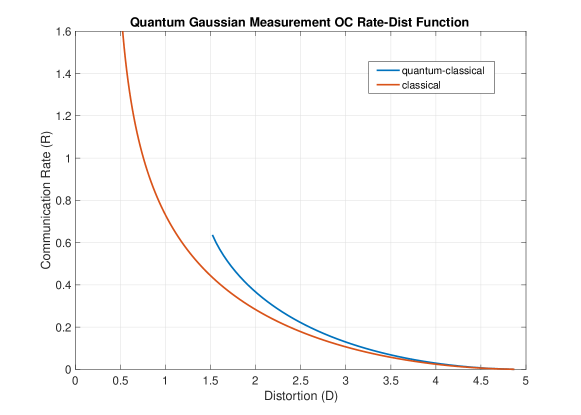
Figure 4: Plot of the OC rate-distortion function of (Blue): the QC Gaussian measurement system with zero mean and marginal covariance matrices in (144), and (Red): the fully classical Gaussian system with Gaussian marginal distributions with zero mean and same covariance matrices as (144).

The simulations are performed using Strawberry fields [72] and Walrus [73] packages and Matlab.

6 Conclusion

We established a Quantum-to-Classical Rate-Limited Optimal Transport problem formulation involving both discrete and continuous-variable quantum systems. We provided a single-letter computable characterization of the performance limits of this problem using quantum information quantities. The performance limit is given by the achievable rate region which is the collection of all communication and common randomness rates $(R,R_{c})$ fulfilling the distortion level in accordance with a generally defined form of distortion observable. Considering a general form of distortion observable in the coding theorem, made it possible to use different distortion measures corresponding to discrete and continuous-variable QC systems. Next, the example of Qubit-Bernoulli, the RLOT was evaluated for the unlimited common randomness and entanglement fidelity distortion measure. For the Gaussian measurement system, by reformatting the quadratic cost operator of [22], we introduced the QC rate-limited Wasserstein distance of order 2. Our Gaussian optimality theorem further showed that the Gaussian RL 2-Wasserstein distance is achieved by the Gaussian measurements. Based on that, the closed-form expressions for the rate-limited QC 2-Wasserstein distance of Gaussian isotropic systems were provided. The conventional 2-Wasserstein distance was also obtained as the special case when $R=\infty$.

As described in the introduction, in the finite-dimensional systems, the fully quantum version of rate-distortion coding has been studied for the memoryless sources in works like [26, 74, 75, 76], and for one-shot setting in [77, 78]. We plan to address as a part of our future work the QC RLOT problem in one-shot settings for both finite-dimensional and continuous-variable systems, in addition to the evaluations of the Quantum Gaussian Measurement systems. Another important line of work that may be of interest is to consider the fully quantum counterpart of these RLOT problems both in asymptotic IID and one-shot regimes in finite-dimensional and continuous-variable settings as well as their evaluations. We also plan to address the applications of these concepts in developing new quantum measure concentration inequalities and their relation to the capacity of the quantum relay channels.

Appendix A Proof of Useful Lemmas

A.1 Proof of Proposition 2

The following lemmas are used in this proof.

Lemma 3.

[79, Proposition 6] Let $\{{\rho^{(n)A}}\}$ be a sequence of states converging to a state ${\rho^{(0)A}}$ (See Section 11.1 of [38]). Also, let $\{M_{n}\}$ be any arbitrary sequence of POVMs weakly converging to a POVM $M_{0}$, with the outcome space $\mathcal{W}$. If either $\absolutevalue{\mathcal{W}}<+\infty$ or $\lim_{n\to\infty}H({\rho^{(n)A}})=H({\rho^{(0)A}})<+\infty$ then $\lim_{n\to\infty}I_{g}(M_{n},{\rho^{(n)A}})=I_{g}(M_{0},{\rho^{(0)A}})$, where $I_{g}(M,\rho)$ is the information gain as defined by Groenwold.

Lemma 4.

The sequence of $\hat{M}_{k_{1}}$ POVMs converges weakly to the $M_{W}$ POVM.

Proof.

See Appendix A.2. ∎

Then the proof of proposition 2 is as follows.

Proof.

To prove the first inequality of (78) we directly use Lemma 3 by Shirokov. To use this lemma in our system, we demonstrate a refined POVM by combining the clipping projection and the measurement POVM $M_{W}$ into, $\hat{M}_{k_{1}}=\left\{\left\{M_{W}(B)\Pi_{k_{1}},B\in\mathcal{B}\right\},I-\Pi_{k_{1}}\right\}$. It is straightforward that this refined POVM is a valid POVM. Next, Lemma 4 proves the weak convergence of this refined POVM. Therefore, by applying Lemma 3 and gentle measurement lemma, it follows that $\lim_{k_{1}\to\infty}I_{g}(R_{k_{1}},W^{\prime}_{k_{1}})=I_{g}(R;W)$. To prove the second rate inequality of (78), we first apply the chain rule for mutual information, $I(W,A_{k_{1}};X_{\bar{k}_{2}})=I(W;X_{\bar{k}_{2}})+I(A_{k_{1}};X_{\bar{k}_{2}}|W)\leq H(A_{k_{1}})+I(W;X_{\bar{k}_{2}})$.

Hence, $I(W,A_{k_{1}};X_{\bar{k}_{2}})-H(A_{k_{1}})\leq I(W;X_{\bar{k}_{2}})\leq I(W,A_{k_{1}};X_{\bar{k}_{2}})$. As $H(A_{k_{1}})$ decays to zero when $k_{1}\to\infty$, from squeeze theorem we have the following limit

$$\lim_{k_{1}\to\infty}I(W,A_{k_{1}};X_{\bar{k}_{2}})=I(W;X_{\bar{k}_{2}}).$$ (145)

Further, applying another chain rule we get

$$I(W,A_{k_{1}};X_{\bar{k}_{2}}) =I(A_{k_{1}};X_{\bar{k}_{2}})+(1-P_{k_{1}})\cdot I(W;X_{\bar{k}_{2}}|A_{k_{1}}=0)+P_{k_{1}}\cdot I(W;X_{\bar{k}_{2}}|A_{k_{1}}=1).$$ (146)

As the clipping region grows to infinity, the probability of clipping decays to zero $\lim_{k_{1}\to\infty}P_{k_{1}}=0$. Then, because $A_{k_{1}}$ is a simple Bernoulli random variable with an arbitrarily small probability, we have $I(A_{k_{1}};X_{\bar{k}_{2}})\leq H(A_{k_{1}})\to 0$. Also for the third term, the following asymptotic bound exists:

$$\lim_{k_{1}\to\infty}P_{k_{1}}\cdot I(W;X_{\bar{k}_{2}}|A_{k_{1}}=1)\leq\lim_{k_{1}\to\infty}P_{k_{1}}\cdot H(X_{\bar{k}_{2}})=0,$$ (147)

where we appealed to the fact that quantized output with limited alphabet has limited entropy.

Finally, consider that $I(W;X_{\bar{k}_{2}}|A_{k_{1}}=0)=I(W^{\prime}_{k_{1}},X^{\prime}_{k_{1},\bar{k}_{2}})$ holds by definition because when the input state is inside the clipping subspace, the system behaves as if no clipping was performed. Combining all together, for any fixed $\bar{k}_{2}$, we have

$$\lim_{k_{1}\to\infty}I(W,A_{k_{1}};X_{\bar{k}_{2}})=\lim_{k_{1}\to\infty}I(W^{\prime}_{k_{1}},X^{\prime}_{k_{1},\bar{k}_{2}}).$$ (148)

Then (145) and (148) together show that for any fixed $\bar{k}_{2}$ we have $\lim_{k_{1}\to\infty}I(W^{\prime}_{k_{1}},X^{\prime}_{k_{1},\bar{k}_{2}})=I(W,X_{\bar{k}_{2}})\leq I(W;X)$, where the inequality follows directly from the Data Processing Inequality and completes the proof. In addition, note that as $k_{2},k_{2}^{\prime}\to\infty$, $X_{\bar{k}_{2}}$ converges weakly to $X$. Therefore, using lower semi-continuity of mutual information [80, 81], combined with the above data-processing inequality we further have $\lim_{k_{2},k_{2}^{\prime}\to\infty}\lim_{k_{1}\to\infty}I(W^{\prime}_{k_{1}},X^{\prime}_{k_{1},\bar{k}_{2}})=\lim_{k_{2},k_{2}^{\prime}\to\infty}I(W,X_{\bar{k}_{2}})=I(W;X)$. ∎

A.2 Proof of Lemma 4

By definition of the weak convergence of operators in [38, Section 11.1], it suffices to show that for each subset $B\in\mathcal{B}$ and any two arbitrary states $\phi,\psi\in\mathcal{H}$, it holds that $\lim_{k_{1}\to\infty}\innerproduct{\psi\Big{|}\hat{M}_{k_{1}}(B)}{\phi}=\innerproduct{\phi|M(B)}{\psi}$. Starting with $I-\Pi_{k_{1}}$, we show that this operator vanishes to zero when $k_{1}\to\infty$, for any $\psi,\phi\in\mathcal{H}$

$$\lim_{k_{1}\to\infty}\Big{|}\innerproduct{\phi|(I-\Pi_{k_{1}})}{\psi}\Big{|} \leq\lim_{k_{1}\to\infty}\norm{(I-\Pi_{k_{1}})\ket{\psi}}_{2}.\norm{(I-\Pi_{k_{1}})\ket{\phi}}_{2}$$

$$=\lim_{k_{1}\to\infty}\sqrt{\innerproduct{\phi|(I-\Pi_{k_{1}})}{\phi}}\cdot\sqrt{\innerproduct{\psi|(I-\Pi_{k_{1}})}{\psi}},$$

where the inequality appeals to Cauchy-Schwartz’s inequality for Hilbert space. By using the definition of the projector operator and Bessel’s inequality and the fact that $\ket{n}$ are orthonormal set, we have $\innerproduct{\phi|\Pi_{k_{1}}}{\phi}=\sum_{n=1}^{k_{1}}|\innerproduct{n}{\phi}|^{2}\leq\norm{\phi}^{2}$. The inequality turns into equality when the orthonormal set is a complete orthonormal basis (Parseval’s identity), which is when $k_{1}\to\infty$. Substituting this into the inner-product expression proves that $\lim_{k_{1}\to\infty}\Big{|}\innerproduct{\phi|(I-\Pi_{k_{1}})}{\psi}\Big{|}=0$. Moreover, for the other operators, we have $\lim_{k_{1}\to\infty}\innerproduct{\phi|M(B)\Pi_{k_{1}}}{\psi}=\lim_{k_{1}\to\infty}\innerproduct{\phi^{\prime}|\Pi_{k_{1}}}{\psi}=\innerproduct{\phi^{\prime}}{\psi}=\innerproduct{\phi|M(B)}{\psi}$, where $\ket{\phi^{\prime}}=M(B)\ket{\phi}$, and the argument is similar to previous operator. These together prove that the sequence of POVMs $\hat{M}_{k_{1}}$ weakly converge to the $M$ POVM.

A.3 Proof of Lemma 1

We condition the average n-letter distortion on the sequence of clipping errors $A_{k_{1}}^{n}$ as follows:

$$d_{n}(R^{n},{\hat{X}}^{n}_{k_{1},\bar{k}_{2}}|\neg E_{ce})=\mathbb{E}_{A_{k_{1}}^{n}|\neg E_{ce}}\left[{d_{n}(R^{n},\hat{X}^{n}_{k_{1},\bar{k}_{2}}|A_{k_{1}}^{n})}\right]$$

$$=\mathbb{E}_{A_{k_{1}}^{n}|\neg E_{ce}}\left[{\frac{1}{n}\sum_{i:A_{i,k_{1}}=1}d(R_{i},\hat{X}_{i,k_{1},\bar{k}_{2}}|A_{k_{1}}^{n})+\frac{1}{n}\sum_{i:A_{i,k_{1}}=0}d(R_{i},\hat{X}_{i,k_{1},\bar{k}_{2}}|A_{k_{1}}^{n})}\right]$$

$$=\mathbb{E}_{T|\neg E_{ce}}\left[{\frac{n-T}{n}d(R,\hat{X}_{\text{local}}|A_{k_{1}}=1)+\frac{T}{n}d_{T}(R_{k_{1}}^{T},\hat{X}^{T}_{k_{1},\bar{k}_{2}})}\right]$$

$$\leq(P_{k_{1}}+\epsilon_{cl})d\left(R,\hat{X}_{\text{local}}|A_{k_{1}}=1\right)+\mathbb{E}_{T|\neg E_{ce}}\left[{d_{T}(R_{k_{1}}^{T},\hat{X}^{T}_{k_{1},\bar{k}_{2}})}\right]$$ (149)

where in the last equality, we generate a local random value $\hat{X}_{\text{local}}$ at Bob’s side for any sample with an asserted error bit $A_{i,k_{1}}=1$. To determine the second term, note that the event $\neg E_{ce}$ means $T\geq t_{\text{min}}$. Then for any value of $\bar{\varepsilon}>0$, by the Theorem 1, for all sufficiently large $n$ (resulting in a sufficiently large value of $t_{\text{min}}$) and for any $t\geq t_{\text{min}}$, we have that $d_{t}(R^{t}_{k_{1}},{X^{\prime}}^{t}_{k_{1},\bar{k}_{2}})\leq d(R_{k_{1}},{X^{\prime}}_{k_{1},\bar{k}_{2}})+\bar{\varepsilon}$, thus,

$$d_{t}(R^{t}_{k_{1}},{\hat{X}}^{t}_{k_{1},\bar{k}_{2}}) \leq d(R_{k_{1}},{X^{\prime}}_{k_{1},\bar{k}_{2}})+\bar{\varepsilon}+\Big{(}d_{t}(R^{t}_{k_{1}},{\hat{X}}^{t}_{k_{1},\bar{k}_{2}})-d_{t}(R^{t}_{k_{1}},{X^{\prime}}^{t}_{k_{1},\bar{k}_{2}})\Big{)}.$$ (150)

The second part of (150) is the distortion caused by the dequantizer block in the receiver. However, we cannot use the triangle inequality to sum up the distortion of the blocks of the system. Instead, we expand the expressions of each term and find the difference. Define $\{\Lambda^{\mathcal{X}^{t}_{\bar{k}_{2}}}_{x^{t}}\}_{x^{t}\in\mathcal{X}^{t}_{\bar{k}_{2}}}$ as the $t$-collective measurement of the $t$-letter discrete coding scheme which generates discrete output sequence with perfect IID pmf $\mu_{X_{\bar{k}_{2}}}$. Also define the continuous measurement POVM $\hat{\Lambda}\equiv\{\hat{\Lambda}(B),B\in\mathcal{B}(\mathcal{X}^{t})\}$ by combining the discrete measurement with the dequantizer optimal transport block, which is expressed for any event $B\subseteq\mathcal{B}(\mathcal{X}^{t})$ by $\hat{\Lambda}(B):=\sum_{x^{t}\in\mathcal{X}_{\bar{k}_{2}}^{t}}\Lambda^{\mathcal{X}^{t}_{\bar{k}_{2}}}_{x^{t}}\pi^{t}_{OT}(B|x^{t}).$

The conditional distribution $\pi_{OT}(.|x^{t})$ for $x^{t}\in\mathcal{X}^{t}_{\bar{k}_{2}}$ representing the dequantizer optimal transport is a memoryless channel because the discrete coding produces IID discrete pmf $\mu_{X_{\bar{k}_{2}}}$ and the final output is required to have IID continuous distribution $\mu_{X}$. For any event $B\subseteq\mathcal{B}(\mathcal{X}^{t})$ it can be expressed by $\pi^{t}_{OT}(B|x^{t})=\mu^{t}_{X}(A\cap{RQ}_{\bar{k}_{2}}(x^{t}))\;/\;\mu^{t}_{X}\left(\mathcal{RQ}_{\bar{k}_{2}}(x^{t})\right),$ where $\mathcal{RQ}_{\bar{k}_{2}}(x^{t})$ is the quantization region of $x^{t}\in\mathcal{X}_{\bar{k}_{2}}^{t}$. Next, the distortion of the discrete coding block for the $i$-th local state is expanded as follows:

$$d(R_{i,k_{1}},X^{\prime}_{i,k_{1},\bar{k}_{2}})=\sum_{x^{t}\in\mathcal{X}^{t}_{\bar{k}_{2}}}\Tr{\Tr_{[t]\setminus i}\left\{\omega_{k_{1}}\Lambda^{\mathcal{X}^{t}_{\bar{k}_{2}}}_{x^{t}}\omega_{k_{1}}\right\}\Delta(x_{i})}$$

$$=\sum_{x_{i}\in\mathcal{X}_{\bar{k}_{2}}}\Tr\{\Tr_{[t]\setminus i}\bigg{\{}\omega_{k_{1}}\bigg{(}\sum_{x^{[t]\setminus i}\in\mathcal{X}^{t-1}_{\bar{k}_{2}}}\Lambda^{\mathcal{X}^{t}_{\bar{k}_{2}}}_{x^{t}}\bigg{)}\omega_{k_{1}}\bigg{\}}\Delta(x_{i})\bigg{\}}=\sum_{x\in\mathcal{X}_{\bar{k}_{2}}}\Tr\{\hat{\rho}^{R_{i}}_{x}\Delta(x)\bigg{\}}\mu_{X_{\bar{k}_{2}}}(x),$$ (151)

where $\omega_{k_{1}}:=\sqrt{\rho_{k_{1}}^{\otimes t}}$ and $\hat{\rho}^{R_{i}}_{x}:=\frac{1}{\mu_{X_{\bar{k}_{2}}}(x)}\Tr_{[t]\setminus i}\bigg{\{}\omega_{k_{1}}\bigg{(}\sum_{x^{[t]\setminus i}\in\mathcal{X}^{t-1}_{\bar{k}_{2}}}\Lambda^{\mathcal{X}^{t}_{\bar{k}_{2}}}_{x^{t}}\bigg{)}\omega_{k_{1}}\bigg{\}}$, is the PMR state of the $i$-th local system after discrete measurement POVM. The state is normalized by $\mu_{X_{\bar{k}_{2}}}(x)$ because the output-constrained coding implies the IID distribution of the output. We further have the distortion of the $i$-th local system up to the output of dequantizer as,

$$d(R_{i,k_{1}},\hat{X}_{i,k_{1},\bar{k}_{2}}) =\int_{\mathcal{X}^{t}}\Tr{\Tr_{[t]\setminus i}\left\{\omega_{k_{1}}\hat{\Lambda}(dz^{t})\omega_{k_{1}}\right\}\Delta(z_{i})}$$

$$=\sum_{x^{t}\in\mathcal{X}^{t}_{\bar{k}_{2}}}\int_{\mathcal{RQ}_{\bar{k}_{2}}(x^{t})}\Tr{\Tr_{[t]\setminus i}\left\{\omega_{k_{1}}\Lambda^{\mathcal{X}^{t}_{\bar{k}_{2}}}_{x^{t}}\pi^{t}_{OT}\Big{(}dz^{t}\Big{|}x^{t}\Big{)}\omega_{k_{1}}\right\}\Delta(z_{i})}$$

$$=\sum_{x_{i}\in\mathcal{X}_{\bar{k}_{2}}}\int_{\mathcal{RQ}_{\bar{k}_{2}}(x_{i})}\Tr{\Tr_{[t]\setminus i}\left\{\omega_{k_{1}}\left(\sum_{x^{[t]\setminus i}}\Lambda^{\mathcal{X}^{t}_{\bar{k}_{2}}}_{x^{t}}\right)\omega_{k_{1}}\right\}\Delta(z_{i})\pi_{OT}(dz_{i}|x_{i})}$$

$$=\sum_{x\in\mathcal{X}_{\bar{k}_{2}}}\Tr{\hat{\rho}^{R_{i}}_{x}\left(\int_{\mathcal{RQ}_{\bar{k}_{2}}(x)}\Delta(z)\pi_{OT}(dz|x)\right)}\mu_{X_{\bar{k}_{2}}}(x),$$ (152)

Then having the expressions (151) and (152), the distortion caused by the optimal transport block is:

$$d_{t}(R_{k_{1}}^{t},\hat{X}_{k_{1},\bar{k}_{2}}^{t})-d_{t}(R_{k_{1}}^{t},{X^{\prime}}^{t}_{k_{1},\bar{k}_{2}}) =\frac{1}{t}\sum_{i=1}^{t}\sum_{x\in\mathcal{X}_{\bar{k}_{2}}}\Tr{\hat{\rho}^{R_{i}}_{x}\left(\int_{\mathcal{RQ}_{\bar{k}_{2}}(x)}\Delta(z)\pi_{OT}(dz|x)-\Delta(x)\right)}\mu_{X_{\bar{k}_{2}}}(x)$$

$$=\frac{1}{t}\sum_{i=1}^{t}\int_{\mathcal{X}}\Tr{\hat{\rho}^{R_{i}}_{Q_{\bar{k}_{2}}(x)}\Big{(}\Delta(x)-\Delta(Q_{\bar{k}_{2}}(x))\Big{)}}\mu_{X}(dx),$$ (153)

Finally, substituting (153) and (150) into (149) provides the following bound

$$d_{n}(R^{n},{\hat{X}}^{n}_{k_{1},\bar{k}_{2}}|\neg E_{ce}) \leq d(R_{k_{1}},X^{\prime}_{k_{1},\bar{k}_{2}})+\bar{\varepsilon}+\varepsilon_{1}(k_{1})+\varepsilon_{2}(n,k_{1},\bar{k}_{2}),$$

where

$$\varepsilon_{1}(k_{1}) :=(P_{k_{1}}+\epsilon_{cl})d\left(R,\hat{X}_{\text{local}}|A_{k_{1}}=1\right),$$ (154)

$$\varepsilon_{2}(n,\bar{k}_{2}) :=\mathbb{E}_{T|\neg E_{ce}}\left[{\frac{1}{T}\sum_{i=1}^{T}\int_{\mathcal{X}}\Tr{\hat{\rho}^{R_{i}}_{Q_{\bar{k}_{2}}(x)}\Big{(}\Delta(x)-\Delta(Q_{\bar{k}_{2}}(x))\Big{)}}\mu_{X}(dx)}\right].$$ (155)

For $\varepsilon_{1}(k_{1})$, by letting $\epsilon_{cl}\leq P_{k_{1}}$ and as a result of uniform integrability, for any $\varepsilon^{\prime}_{1}>0$ there exists a sufficiently large $k_{1}$ such that $\varepsilon_{1}(k_{1})\leq\varepsilon^{\prime}_{1}$. For $\varepsilon_{2}(n,\bar{k}_{2})$, the integral inside the expectation is split into the inside and outside the clipping interval and then bounded by

$$\varepsilon_{2}(n,\bar{k}_{2}) =\mathbb{E}_{T|\neg E_{ce}}\left[{\frac{1}{T}\sum_{i=1}^{T}\int_{-2^{k_{2}}}^{2^{k_{2}}}\Tr{\hat{\rho}^{R_{i}}_{Q_{\bar{k}_{2}}(x)}\Big{(}\Delta(x)-\Delta(Q_{\bar{k}_{2}}(x))\Big{)}}\mu_{X}(dx)}\right]$$

$$+\mathbb{E}_{T|\neg E_{ce}}\left[{\frac{1}{T}\sum_{i=1}^{T}\int_{\mathcal{X}\setminus[-2^{k_{2}},2^{k_{2}}]}\Tr{\hat{\rho}^{R_{i}}_{Q_{\bar{k}_{2}}(x)}\Big{(}\Delta(x)-\Delta(Q_{\bar{k}_{2}}(x))\Big{)}}\mu_{X}(dx)}\right]\leq\varepsilon_{21}(k_{1})+\varepsilon_{22}(n,\bar{k}_{2})$$

where

$$\varepsilon_{21}(k_{1}) :=\int_{-2^{k_{2}}}^{2^{k_{2}}}\norm{\Delta(x)-\Delta(Q_{\bar{k}_{2}}(x))}_{1}\mu_{X}(dx),$$ (156)

$$\varepsilon_{22}(n,\bar{k}_{2}) :=\mathbb{E}_{T|\neg E_{ce}}\left[{\frac{1}{T}\sum_{i=1}^{T}\int_{\mathcal{X}\setminus[-2^{k_{2}},2^{k_{2}}]}\Tr{\hat{\rho}^{R_{i}}_{Q_{\bar{k}_{2}}(x)}\Big{(}\Delta(x)-\Delta(Q_{\bar{k}_{2}}(x))\Big{)}}\mu_{X}(dx)}\right].$$ (157)

To obtain $\varepsilon_{21}(k_{1})$ we used Holder’s inequality on the first term and the fact that the PMR state $\hat{\rho}_{x}^{R_{i}}$ for $x\in\mathcal{X}_{\bar{k}_{2}}$ is a state of finite-dimensional space. The expectation term is excluded because the resulting term is not a function of $T$. Then the first term above can be made arbitrarily small to any $\varepsilon^{\prime}_{21}$ by choosing a large enough $k_{1}$, due to the continuity of the $\Delta(x)$ operator ($\varepsilon_{21}(k_{1})\leq\varepsilon^{\prime}_{21}$).

In the second term $\varepsilon_{22}(n,\bar{k}_{2})$, for the inner integral, by the definition of the uniform integrability, regardless of the index $i$, for an arbitrarily small value $\varepsilon^{\prime}_{22}>0$ there exists a large enough $k_{2}$ such that

$$\int_{\mathcal{X}\setminus[-2^{k_{2}},2^{k_{2}}]}\Tr{\hat{\rho}^{R_{i}}_{Q_{\bar{k}_{2}}(x)}\Big{(}\Delta(x)-\Delta(Q_{\bar{k}_{2}}(x))\Big{)}}\mu_{X}(dx)\leq\varepsilon^{\prime}_{22}\quad\text{for }i=1,\cdots,T.$$ (158)

Then for any value of $n$ we have that $\varepsilon_{22}(n,\bar{k}_{2})\leq\mathbb{E}_{T|\neg E_{ce}}\left[{\frac{1}{T}\sum_{i=1}^{T}\varepsilon^{\prime}_{22}}\right]=\varepsilon^{\prime}_{22}$.

Finally putting it all together gives the single-letter upper bound

$$d_{n}(R^{n},{\hat{X}}^{n}_{k_{1},\bar{k}_{2}}|\neg E_{ce}) \leq d(R_{k_{1}},X^{\prime}_{k_{1},\bar{k}_{2}})+\bar{\varepsilon}+\varepsilon^{\prime}_{21}+\varepsilon^{\prime}_{22}.$$ (159)

where $\bar{\varepsilon}>0$ can be made arbitrarily small given sufficiently large $n$ and $\varepsilon^{\prime}_{21},\varepsilon^{\prime}_{22}$ can be made arbitrarily small given sufficiently large $k_{1},k_{2}$.

A.4 Uniform Integrability of Gaussian Measurement System

The distortion function (107) can be expressed in a different form as follows:

$$d(\rho_{A},\Lambda) =\frac{1}{2s}\sum_{i=1}^{2s}\mathbb{E}_{Z}\left[{\Tr{\rho_{Z}R_{i}^{2}}+\Tr{\rho_{Z}}Z_{i}^{2}-2\Tr{\rho_{Z}R_{i}}Z_{i}}\right]:=d(\rho_{Z},\pi_{Z}).$$ (160)

Lemma 5.

Considering a Gaussian quantum Optimal transport measurement system comprised of a Gaussian source state $\rho$ and a Gaussian output distribution $\pi_{Z}$, with the PMR ensemble $\{\{\rho_{z}\}_{z\in\mathcal{Z}},\pi_{Z}\}$. For any set of projection operators $\Pi_{Z}$ such that $\mathbb{E}_{Z}\left[{\rho_{Z}\Pi_{Z}}\right]\leq\delta$, we have that $d(\Pi_{Z}\rho_{Z}\Pi_{Z},\pi_{Z})\leq f(\delta),$ where $f(\delta)\downarrow 0$ as $\delta\downarrow 0$.

Proof.

The proof follows a nested use of the Cauchy-Schwartz inequality. The distortion of the unnormalized projected state is expanded as

$$d(\Pi_{Z}\rho_{Z}\Pi_{Z},\pi_{Z})=\frac{1}{2s}\sum_{i=1}^{2s}\mathbb{E}_{Z}\left[{\Tr{\Pi_{Z}\rho_{Z}\Pi_{Z}R_{i}^{2}}+\Tr{\Pi_{Z}\rho_{Z}}Z_{i}^{2}-2\Tr{\Pi_{Z}\rho_{Z}\Pi_{Z}R_{i}}Z_{i}}\right].$$ (161)

We further examine each term separately. The operation $\langle M,N\rangle=\Tr{M^{\dagger}N}$ is the Hilbert-Schmidt inner product, then it satisfies the Cauchy-Schwartz inequality. Thus, for the first term of (161) we have,

$$\Tr{\Pi_{Z}\rho_{Z}\Pi_{Z}R_{i}^{2}} =\Tr{\sqrt{\rho_{Z}}\Pi_{Z}R_{i}^{2}\Pi_{Z}\sqrt{\rho_{Z}}}\leq\sqrt{\Tr{\rho_{Z}\Pi_{Z}}}\sqrt{\Tr{\Pi_{Z}\rho_{Z}\Pi_{Z}R_{i}^{4}}}.$$

Then we use another round of Cauchy-Schwartz inequality for its classical expectation:

$$\mathbb{E}_{Z}\left[{\sqrt{\Tr{\rho_{Z}\Pi_{Z}}}\sqrt{\Tr{\Pi_{Z}\rho_{Z}\Pi_{Z}R_{i}^{4}}}}\right] \leq\sqrt{\mathbb{E}_{Z}\left[{\Tr{\rho_{Z}\Pi_{Z}}}\right]}\sqrt{\mathbb{E}_{Z}\left[{\Tr{\Pi_{Z}\rho_{Z}\Pi_{Z}R_{i}^{4}}}\right]}$$

$$\leq\sqrt{\delta}\sqrt{\mathbb{E}_{Z}\left[{\Tr{\Pi_{Z}\rho_{Z}\Pi_{Z}R_{i}^{4}}}\right]}:=f_{1,i}(\delta).$$ (162)

By the Gaussian Optimality Theorem 5, the optimal PMR states $\rho_{Z}$ corresponding to the rate-limited optimal transport measurement are all Gaussian quantum states. Then in the above inequality, $f_{1,i}(\delta)\downarrow 0$ as $\delta\downarrow 0$ because the fourth moment of a Gaussian quantum source state $\rho_{Z}$ is finite, and thus, the moments of its projection by $\Pi_{Z}$ will still remain finite.

The second term of (161) is upper-bounded by the Cauchy-Schwartz inequality as:

$$\mathbb{E}_{Z}\left[{Z_{i}^{2}\Tr{\Pi_{Z}\rho_{Z}}}\right] \leq\sqrt{\mathbb{E}_{Z}\left[{Z_{i}^{4}}\right]}\sqrt{\mathbb{E}_{Z}\left[{\left(\Tr{\Pi_{Z}\rho_{Z}}\right)^{2}}\right]}$$

$$\leq\sqrt{\mathbb{E}_{Z}\left[{Z_{i}^{4}}\right]}\sqrt{\mathbb{E}_{Z}\left[{\Tr{\Pi_{Z}\rho_{Z}}}\right]}\leq\sqrt{\mathbb{E}_{Z}\left[{Z_{i}^{4}}\right]}\sqrt{\delta}:=f_{2,i}(\delta)$$ (163)

where we used the fact that the fourth moment of the output Gaussian distribution $\pi_{Z}$ is finite. The third term of (161) follows a similar approach to the above steps:

$$-\mathbb{E}_{Z}\left[{\Tr{\Pi_{Z}\rho_{Z}\Pi_{Z}R_{i}}Z_{i}}\right] \leq\sqrt{\mathbb{E}\left[{Z_{i}^{2}}\right]}\sqrt{\mathbb{E}_{Z}\left[{\left(\Tr{\Pi_{Z}\rho_{Z}\Pi_{Z}R_{i}}\right)^{2}}\right]}$$

$$\leq\sqrt{\mathbb{E}\left[{Z_{i}^{2}}\right]}\sqrt{\mathbb{E}_{Z}\left[{\Tr{\rho_{Z}\Pi_{Z}}\Tr{\Pi_{Z}\rho_{Z}\Pi_{Z}R_{i}^{2}}}\right]}$$

$$\leq\sqrt{\mathbb{E}\left[{Z_{i}^{2}}\right]}\sqrt[4]{\mathbb{E}_{Z}\left[{\left(\Tr{\rho_{Z}\Pi_{Z}}\right)^{2}}\right]\cdot\mathbb{E}_{Z}\left[{\left(\Tr{\Pi_{Z}\rho_{Z}\Pi_{Z}R_{i}^{2}}\right)^{2}}\right]}$$

$$\leq\sqrt[4]{\delta}\sqrt{\mathbb{E}\left[{Z_{i}^{2}}\right]}\sqrt[4]{\mathbb{E}_{Z}\left[{\left(\Tr{\Pi_{Z}\rho_{Z}\Pi_{Z}R_{i}^{2}}\right)^{2}}\right]}:=f_{3,i}(\delta)$$ (164)

Putting all the bounds above together shows that the projected distortion in (161) is upper-bounded by a continuous function $f(\delta)$ as follows, where $f(\delta)\downarrow 0$ as $\delta\downarrow 0$. Hence by definition, the Gaussian measurement system is Uniformly integrable, $d(\Pi_{z}\rho_{z}\Pi_{z},\pi_{z})\leq\frac{1}{2s}\sum_{i=1}^{2s}\left(f_{1,i}(\delta)+f_{2,i}(\delta)+2f_{3,i}(\delta)\right):=f(\delta)$. ∎

Appendix B Proof of Theorem 3

We start with the optimization problem in (89) and change the variable of optimization to $N=\sqrt{\rho}M_{0}\sqrt{\rho}$, which is the unnormalized conditional PMR state given outcome zero. The optimization problem reduces to the following form

$$\min_{N}{\quad\Tr{N\ln(N/q_{0})}+\Tr{(\rho-N)\ln(\frac{\rho-N}{1-q_{0}})}},$$ (165)

$$\text{such that,}\;\bra{0}\sqrt{\rho}N\sqrt{\rho}\ket{0}+\bra{1}\sqrt{\rho}(\rho-N)\sqrt{\rho}\ket{1}\geq 1-D,$$ (166)

$$\Tr{N}=q_{0},\quad 0\preceq N\preceq\rho.$$ (167)

This is a convex optimization problem, as the objective function comprises negative entropy functions that are concave, and the constraint is linear. The distortion constraint (166) is further simplified to

$$\Tr{NG}\geq 1-D-\innerproduct{1|\rho^{2}}{1},\quad G:=\sqrt{\rho}\begin{bmatrix}1&0\\ 0&-1\end{bmatrix}\sqrt{\rho}.$$ (168)

We first obtain the zero-crossing point $D_{R_{0}}$ which is the threshold that any distortion value $D\geq D_{R_{0}}$, is achieved by zero communication rate ($R=0$). Setting the rate to zero $I(R;X)=H(\rho)-q_{0}H(\hat{\rho}_{0})-q_{1}H(\hat{\rho}_{1})=0$ gives $\hat{\rho}_{0}=\hat{\rho}_{1}=\rho$. The measurement POVMs corresponding to these PMR states are $M_{0}=q_{0}I,\;M_{1}=(1-q_{0})I$. Substituting $\hat{\rho}_{0}=\hat{\rho}_{1}=\rho$ in the distortion constraint gives the zero-crossing point $D_{R_{0}}:=1-q_{0}\innerproduct{0}{\rho^{2}|0}-(1-q_{0})\innerproduct{1}{\rho^{2}|1}$.

Next, in the non-zero rate region $D_{OT}\leq D\leq D_{R_{0}}$, the distortion constraint is active. Note that $D_{OT}$ is the optimal transportation cost which is the minimum feasible distortion possible for the system.

We first show here that the optimal solution of $N$ is of the form presented in (94). Recall that the convex problem (165) is on the domain of positive semi-definite Hermitian matrices $N\in\mathcal{S}^{n}_{+}$, and has a fixed trace $\Tr{N}=q_{0}$. So it can be initially considered as the following matrix form:

$$N=\begin{bmatrix}n&n_{\text{off}}\\ n_{\text{off}}^{*}&q_{0}-n\end{bmatrix},$$ (169)

where $n\in\mathbb{R}^{+}$ and $n_{\text{off}}\in\mathbb{C}$. Further, the PSD constraints of (167) reduce to $\det(N)\geq 0$, and $\det(\rho-N)\geq 0$, and $0\leq\Tr{N}\leq 1$. Thus we have

$$|n_{\text{off}}|^{2}\leq n(q_{0}-n),\qquad |\rho_{2}-n_{\text{off}}|^{2}\leq(\rho_{1}-n)(1-\rho_{1}-q_{0}+n).$$ (170)

Next, by examining the objective function (165) and the constraints, we observe a symmetry in $n_{\text{off}}$ values along the real and imaginary parts of the complex plain. Note that the first term in (165) is a function of eigenvalues of matrix $N$ which only depends on $|n_{\text{off}}|$. Similarly, the second term is only a function of $|\rho_{2}-n_{\text{off}}|$. These two expressions can be illustrated as two circles in the complex plane of $n_{\text{off}}$, which are symmetrical w.r.t. the direction of the vector $\rho_{2}$ in this complex plane. Moreover, by representing $G$ in the following matrix elements format:

$$G:=\begin{bmatrix}g_{1}&\frac{g_{2}}{|\rho_{2}|}\rho_{2}\\ \frac{g_{2}}{|\rho_{2}|}\rho_{2}^{*}&g_{3}\end{bmatrix}=\frac{1}{1+2k}\begin{bmatrix}(\rho_{1}+k)^{2}-|\rho_{2}|^{2}&(2\rho_{1}-1)\rho_{2}\\ b(2\rho_{1}-1)\rho_{2}^{*}&|\rho_{2}|^{2}-(1-\rho_{1}+k)^{2}\end{bmatrix},$$

with $k:=\sqrt{\det{\rho}}$, and (169), we can rewrite the LHS of distortion constraint (168) as

$$\Tr{NG}=(g_{1}-g_{3})n+\frac{2g_{2}}{|\rho_{2}|}\Re{n_{\text{off}}\,\rho^{*}_{2}}+q_{0}g_{3}\geq 1-D-\innerproduct{1|\rho^{2}}{1}.$$

By expanding the term $\Re{n_{\text{off}}\,\rho^{*}_{2}}$ in above expression, the distortion constraint becomes

$$\Re{n_{\text{off}}}\Re{\rho_{2}}+\Im{n_{\text{off}}}\Im{\rho_{2}}+f(n,q_{0},\rho)\geq 0,$$

where $f(n,q_{0},\rho)$ is a function comprised of the remaining terms. This is a half-plane in the complex plane of $n_{\text{off}}$, which is orthogonal to the symmetry line $\rho_{2}$. Therefore, the objective function and all the constraints are symmetric w.r.t. the line $\rho_{2}$ in the complex plane. In view of the fact that the problem is a convex program, the solution must occur on the line of symmetry. This means the optimal solution has the shape of the matrix described in (94), where $n,s\in\mathbb{R}$ are the variables of optimization. Therefore, by rewriting the distortion constraint and the objective function as functions of $n$ and $s$ we arrive at the following optimization problem:

$$\min_{n,s} \sum_{i=1,2}\lambda_{N_{i}}(n,s)\ln(\lambda_{N_{i}}(n,s)/q_{0})+\sum_{i=1,2}\lambda_{d_{i}}(n,s)\ln(\lambda_{d_{i}}(n,s)/(1-q_{0}))$$

such that, $$\Big{(}g_{1}-g_{3}\Big{)}n+\Big{(}2g_{2}\Big{)}s+\Big{(}q_{0}g_{3}+\innerproduct{1|\rho^{2}}{1}-1+D\Big{)}\geq 0$$

where $n,s\in\mathbb{R}$. The terms $\lambda_{N_{1},N_{2}}(n,s)=\frac{q_{0}}{2}\pm E_{1}(n,s)$ and $\lambda_{d_{1},d_{2}}(n,s)=\frac{1-q_{0}}{2}\pm E_{2}(n,s)$ are the eigenvalues of $N$ and $\rho-N$ respectively, with $E_{1}(n,s)$ and $E_{2}(n,s)$ defined in (95).

We solve by substituting the linear constraint into the objective function, then taking the derivative w.r.t. $n$ and equating it to zero. The final solution becomes in the form of the following transcendental system of equations of $n,s$ which provides the optimal values $n_{opt}$ and $s_{opt}$:

$$\frac{-as+b(n-q_{0}/2)}{E_{1}}\ln{\frac{q_{0}/2+E_{1}}{q_{0}/2-E_{1}}}+\frac{-a(s-|\rho_{2}|)+b(n-\rho_{1}+\frac{1-q_{0}}{2})}{E_{2}}\ln{\frac{\frac{1-q_{0}}{2}+E_{2}}{\frac{1-q_{0}}{2}-E_{2}}}=0,$$

$$\bigg{(}1-\frac{4|\rho_{2}|^{2}}{1+2k}\bigg{)}n+\bigg{(}\frac{2|\rho_{2}|(2\rho_{1}-1)}{1+2k}\bigg{)}s+\bigg{(}q_{0}\left(\rho_{1}-1+\frac{2|\rho_{2}|^{2}}{1+2k}\right)+\innerproduct{1|\rho^{2}}{1}-1+D\bigg{)}=0.$$

Appendix C Proof of Theorem 4

To find the optimal transportation cost $D_{OT}$ of the Qubit system, we assume having an unlimited available rate and find the minimum possible distortion. In this case, the problem reduces to

$$D_{OT}:=\min_{M_{0},M_{1}}\; 1-\sum_{x}\innerproduct{x|\rho M_{x}\rho}{x},\quad\text{such that: }\; \Tr{M_{0}\rho}=q_{0},\quad M_{0}+M_{1}=I,\quad M_{0},M_{1}\geq 0.$$

Note that we used the same argument as in Appendix A to remove the transpose operator from the formulations. Then again a change of variable $N:=\sqrt{\rho}M_{0}\sqrt{\rho}$ reduces the problem to the following semi-definite programming: $\min_{N}\quad 1-\innerproduct{1|\rho^{2}}{1}-\Tr{NG},$ such that $\;\Tr{N}=q_{0}$, and $0\preceq N\preceq\rho.$

Similar to the rate-distortion problem in Appendix B, the symmetry requires the optimal solution $N_{OT}$ to be in the matrix form described in (94). With this assumption, the problem reduces to the scalar optimization below:

$$\min_{n,s}f_{0}(n,s) :=-(g_{1}-g_{3})n-(2g_{2})s+1-q_{0}g_{3}-\innerproduct{1|\rho^{2}}{1},$$

$$\text{such that, }\;f_{1}(n,s) :=\left(n-\frac{q_{0}}{2}\right)^{2}+s^{2}-\left(\frac{q_{0}}{2}\right)^{2}\leq 0,$$

$$f_{2}(n,s) :=\left(n-\left(\rho_{1}-\frac{1-q_{0}}{2}\right)\right)^{2}+(s-|\rho_{2}|)^{2}-\left(\frac{1-q_{0}}{2}\right)^{2}\leq 0.$$

This is a quadratic-constrained linear programming which is a convex problem. The Lagrangian function is $\mathcal{L}(n,s,\lambda_{1},\lambda_{2})=f_{0}(n,s)+\lambda_{1}f_{1}(n,s)+\lambda_{2}f_{2}(n,s)$, with $\lambda_{1,2}\geq 0$. Then by taking the partial derivatives with respect to $n,s$ and equating to zero, we obtain the optimal variables as a function of $\lambda_{i}$ Lagrange multipliers,

$$n_{opt}(\lambda_{1},\lambda_{2})=\frac{a+q_{0}\lambda_{1}+2(\rho_{1}-\frac{1-q_{0}}{2})\lambda_{2}}{2(\lambda_{1}+\lambda_{2})},\quad s_{opt}(\lambda_{1},\lambda_{2})=\frac{b+2\lambda_{2}|\rho_{2}|}{2(\lambda_{1}+\lambda_{2})}.$$ (171)

Then by substituting the above expressions in the complementary slackness conditions

$$\lambda_{1}f_{1}\Big{(}n_{opt}(\lambda_{1},\lambda_{2}),\,s_{opt}(\lambda_{1},\lambda_{2})\Big{)}=0,\quad\lambda_{2}f_{2}\Big{(}n_{opt}(\lambda_{1},\lambda_{2}),\,s_{opt}(\lambda_{1},\lambda_{2})\Big{)}=0,\quad\lambda_{1,2}\geq 0,$$

the following solutions are the results of these separate scenarios.

1. Minimum happens at $f_{2}$ circle ($\lambda_{1}=0,\;\lambda_{2}\neq 0$): Because $\lambda_{2}\neq 0$, then $f_{2}(n_{opt},s_{opt})=0$. This results in $\lambda_{2}=\frac{\sqrt{a^{2}+b^{2}}}{1-q_{0}}$. Substituting $\lambda_{1,2}$ into (171) and then substituting the obtained $n_{opt}$ and $s_{opt}$ into objective function gives,

   $$D_{OT} =q_{0}(1-\rho_{1})+\det(\rho)+\frac{1-q_{0}}{2}\left(1-\sqrt{1-4|\rho_{2}|^{2}}\right).$$

   Also, substituting the $n_{opt}$ and $s_{opt}$ values into $f_{1}(n_{opt},s_{opt})\leq 0$ provides the conditions required for this scenario: $\frac{1-q_{0}}{2}+\frac{1-q_{0}}{\sqrt{a^{2}+b^{2}}}\left(a(\rho_{1}-\frac{1}{2})+b|\rho_{2}|\right)\leq\det(\rho).$

2. Minimum happens at $f_{1}$ circle ($\lambda_{1}\neq 0,\lambda_{2}=0$): Because $\lambda_{1}\neq 0$, then $f_{1}(n_{opt},s_{opt})=0$. This results in $\lambda_{1}=\frac{\sqrt{a^{2}+b^{2}}}{q_{0}}$. Again, substituting these $\lambda_{1,2}$ into (171) gives,

   $$D_{OT} =(1-q_{0})\rho_{1}+\det(\rho)+\frac{q_{0}}{2}\left(1-\sqrt{1-4|\rho_{2}|^{2}}\right).$$

   Also, substituting the corresponding $n_{opt}$ and $s_{opt}$ values into $f_{2}(n_{opt},s_{opt})\leq 0$ provides the conditions required for this scenario: $\frac{q_{0}}{2}-\frac{q_{0}}{\sqrt{a^{2}+b^{2}}}\left(a(\rho_{1}-\frac{1}{2})+b|\rho_{2}|\right)\leq\det(\rho)$.

3. Minimum happens at intersection of circles ($\lambda_{1}\neq 0,\lambda_{2}\neq 0$): If neither of the conditions of the above scenarios is satisfied, then the result happens at the intersection of two circles $f_{1}(n,s)=0$ and $f_{2}(n,s)=0$, which results in the following expressions under separate conditions:

   • If $a\geq b$, then $s_{opt}=\frac{2B+q_{0}A+A\sqrt{\Delta}}{2(1+A^{2})}$, and $n_{opt}=\frac{q_{0}-2AB+\sqrt{\Delta}}{2(1+A^{2})}$.

   • If $a<b$, then $s_{opt}=\frac{2B+q_{0}A-A\sqrt{\Delta}}{2(1+A^{2})}$, and $n_{opt}=\frac{q_{0}-2AB-\sqrt{\Delta}}{2(1+A^{2})}$.

   where $A:=\frac{1-2\rho_{1}}{2|\rho_{2}|},\quad B:=\frac{\rho_{1}q_{0}-\det(\rho)}{2|\rho_{2}|},\quad\Delta:=q_{0}^{2}-4B^{2}-4q_{0}AB$.

   Then by substituting the above optimal values in $f_{0}(n_{opt},s_{opt})$ gives the optimal transportation cost $D_{OT}=1-q_{0}g_{3}-\innerproduct{1|\rho^{2}}{1}-an_{opt}-bs_{opt}$.

Appendix D Proof of Theorem 8

Recall from subsection 5.1.1 that for the one-mode system, $\absolutevalue{\Delta^{-1}\Sigma_{N}}=\sqrt{\det{\Sigma_{N}}}I_{2\times 2}$. Then in the objective function (133), we can simplify $\frac{1}{2}\text{Sp }g\left(\absolutevalue{\Delta^{-1}\Sigma_{N}}-\frac{I}{2}\right)=g\left(\sqrt{\det{\Sigma_{N}}}-1/2\right)$. We further change the variable of optimization to $X:=\left(\Sigma_{Z}^{1/2}(\Sigma_{\rho}-\Sigma_{N})\Sigma_{Z}^{1/2}\right)^{1/2}$. This gives the noise covariance $\Sigma_{N}=\Sigma_{\rho}-\Sigma_{Z}^{-1/2}X^{2}\Sigma_{Z}^{-1/2}$. Then the optimization problem for the one-mode system is equivalent to

$$\min_{X}\; \left[\Theta(X):=-g\left(\sqrt{\frac{\det{\Sigma-X^{2}}}{\det{\Sigma_{Z}}}}-\frac{1}{2}\right)\right],$$ (172)

such that: $$c\leq\mathrm{Sp}\left(X\right),$$ (173)

$$0\leq X\leq\left(\Sigma_{Z}^{1/2}\left(\Sigma_{\rho}\pm\frac{i}{2}\Delta\right)\Sigma_{Z}^{1/2}\right)^{1/2},$$ (174)

where $\Sigma:=\Sigma_{Z}^{1/2}\Sigma_{\rho}\Sigma_{Z}^{1/2}$ and $c=D_{\text{max}}-D$.

Note that the inequality $\pm\frac{i}{2}\Delta\leq\Sigma_{N}$ implies that $0\leq\Sigma_{N}$. This in turn implies that $X^{2}\leq\Sigma$. Then on this region $\Sigma\geq X^{2}$, the term $\Sigma-X^{2}$ is a concave and decreasing function of $X\in S^{2}_{+}$ in the generalized matrix inequality sense [82]. We also have that $\det{Y}^{1/n}$ is concave for $Y\in S_{++}^{n}$ [82, Exercise 3.18]. Applying the composition rule, the term inside the $g(.)$ function is convex. Then by the fact that $-g(.)$ is a convex function, it follows that the optimization problem is convex and can be solved using KKT conditions. The Lagrangian function is $L(X)=\Theta(X)-\Tr{\Lambda X^{2}}+\Tr{\Pi X^{2}}-\pi\mathrm{Sp}\left(X\right)$. We develop the KKT conditions,

$$\frac{1}{2}\phi(X)\cdot\log\frac{\phi(X)+1/2}{\phi(X)-1/2}\left[(\Sigma-X^{2})^{-1}X+X(\Sigma-X^{2})^{-1}\right]-\Lambda X-X\Lambda+\Pi X+X\Pi =\pi I,$$ (175)

$$\Lambda X^{2}=0,\quad\Lambda \geq 0,$$ (176)

$$\Pi\left(X^{2}-\Sigma\pm\frac{i}{2}\Sigma_{Z}^{1/2}\Delta\Sigma_{Z}^{1/2}\right)=0,\quad\Pi \geq 0,$$ (177)

$$\pi(\mathrm{Sp}\left(X\right)-c)=0,\quad\pi \geq 0,$$ (178)

where $\phi(X):=\sqrt{\frac{\det{\Sigma-X^{2}}}{\det{\Sigma_{Z}}}}$. The constraint (174) is equivalent to the following two inequalities, $\Tr{X^{2}}\leq\Tr{\Sigma}$, and $\det{\Sigma-X^{2}}\geq\frac{1}{4}\det{\Sigma_{Z}}$. Note that the second inequality above is the feasibility condition of the objective function $\Theta(X)$ and is always satisfied inside the domain. Also, the first inequality is satisfied if $X^{2}\leq\Sigma$. Therefore, under this condition, $\Pi=0$ in the constraint (177).

Next we restrict ourself to the solutions of the form $X=U\text{diag}(x_{i})U^{T}$, where $X$ has the same diagonalization as $\Sigma=U\text{diag}(\sigma_{i}^{2})_{i=1:2}U^{T}$, with $0\leq x_{i}\leq{\sigma_{i}}$. This reduces the KKT conditions to the following system of equations:

$$\phi(X)\cdot\log\frac{\phi(X)+1/2}{\phi(X)-1/2}\frac{x_{i}}{\sigma_{i}^{2}-x_{i}^{2}} =\pi,\quad\text{for }i=1,2$$ (179)

$$\sum_{i}x_{i} =c,\quad\pi\geq 0.$$ (180)

The term $\phi(X)$ does not depend on the index $i$, and therefore, it is just a scaling of $\pi$ which can be absorbed in $\tilde{\pi}=\pi\left(\phi(X)\log\frac{\phi(X)+1/2}{\phi(X)-1/2}\right)^{-1}$. This gives the final solution by the system of equations in (139). It suffices to show that for any given $c_{\text{min}}<c<c_{\text{max}}$, there exists a solution in the form of the equations in (139). Isolating the equality for $x_{i}$ gives $x_{i}=-\frac{1}{2\tilde{\pi}}+\sqrt{(\frac{1}{2\tilde{\pi}})^{2}+\sigma_{i}^{2}}$, for $i=1,2$, which is always valid inside the domain of $x_{i}$. Then by defining $y:=1/(2\tilde{\pi})$, we rewrite the second equation as a function of $y$,

$$f(y):=-ny+\sum_{i=1}^{2}\sqrt{y^{2}+\sigma_{i}^{2}}=c.$$ (181)

Recall that $c=D_{\text{max}}-D$ and $D\in(D_{\text{OT}},D_{\text{max}})$. Therefore, $c_{\text{min}}=0$. The value of $c_{\text{max}}$ corresponds to $D_{\text{OT}}$ which is the Wasserstein distance of the QC system, implied by the feasibility constraint (174).

We next provide a loose upper bound $\hat{c}_{\text{max}}>>c_{\text{max}}$ by relaxing the constraint to $X^{2}\leq\Sigma$. Therefore, ${\hat{c}}_{\text{max}}=\mathrm{Sp}\left(\Sigma^{1/2}\right)=\sum_{i}\sigma_{i}$. As $c_{\text{min}}=0$ results in $y=\infty$ and $c_{\text{max}}=\sum_{i}\sigma_{i}$ results in $y=0$, then both have valid solutions. Further, $f(y)$ function is a monotonically decreasing function of $y$, therefore, there is a one-to-one correspondence between values of $c\in(c_{\text{min}},\hat{c}_{\text{max}})$ and the values of $y\in(0,\infty)$. Thus, for any feasible value of $c\in(c_{\text{min}},{\hat{c}}_{\text{max}})$, there exists a solution of the form (139). This approach is similar to the solution in the classical case proved in [83].

Next, the following optimization problem obtains the Wasserstein distance $D_{OT}$,

$$D_{OT}=\min_{X^{\prime}}D_{\text{max}}-\mathrm{Sp}\left(X^{\prime}\right),\quad\text{such that:}\;\pm\frac{i}{2}\Delta\leq\Sigma_{N}\leq\Sigma_{\rho}.$$ (182)

For the case of one-mode, similar to the approach above, by setting $X=U\text{diag}[y_{1},y_{2}]U^{T}$, this optimization problem reduces to maximizing $\sum_{i}y_{i}$ subject to constraint $\prod_{i=1}^{2}(\sigma_{i}^{2}-y_{i}^{2})\geq\frac{1}{4}\det{\Sigma_{Z}}$ which results in (140).

Appendix E Proof of Cardinality Bound

Here, we provide a cardinality bound for the sample space of the intermediate system $\mathcal{W}$. We start by introducing the QC version of the classical support lemma [84]:

Lemma 6.

(Quantum-Classical Support Lemma) Let $\mathcal{P}\subseteq\mathcal{G}(\mathcal{H}_{A})$ be a compact and connected subset of density operators on finite-dimensional Hilbert space $\mathcal{H}_{A}$, and let $\mathcal{W}$ be an arbitrary set. Further, let $\{\rho_{w}\}_{w\in\mathcal{W}}\in\mathcal{P}$ be a collection of (conditional) density operators. Let $g_{j}(\rho),j=1,...,J$ be a collection of real-valued continuous functions of quantum states $\mathcal{P}$. For every random variable $W$ with probability measure $F(w)$ defined on $\mathcal{W}$, there exist a random variable $W^{\prime}$ defined on $\mathcal{W}^{\prime}$ with PMF $P_{W^{\prime}}$ with $|\mathcal{W}^{\prime}|\leq J$ and a collection of conditional density operators $\tilde{\rho}_{w^{\prime}}\in\mathcal{P}$ indexed by $w^{\prime}\in\mathcal{W}^{\prime}$ such that:

$$\int_{\mathcal{W}}g_{j}(\rho_{w})dF(w)=\sum_{w^{\prime}\in\mathcal{W}^{\prime}}g_{j}(\tilde{\rho}_{w^{\prime}})P_{W^{\prime}}(w^{\prime}),\quad\text{for }j=1,...,J.$$ (183)

Proof.

First note that the set of density operators $\mathcal{G}(\mathcal{H}_{A})$ on finite-dimensional Hilbert space $\mathcal{H}_{A}$ is compact under weak topology. Further, it is connected because it is a convex set. Then the lemma follows directly from the Fenchel-Eggleston-Caratheodory Theorem [84]. ∎

Assume having a composite QC state $\tau^{RWX}\in\mathcal{G}(\mathcal{H}_{R}\otimes\mathcal{H}_{W}\otimes\mathcal{H}_{X})$ forming a quantum Markov chain $R-W-X$ with the PMR ensemble $\{\hat{\rho}_{w},P_{W}(w)\}_{w\in\mathcal{W}}$ with an arbitrary discrete alphabet $\mathcal{W}$ as the intermediate outcomes, and the classical channel $P_{X|W}$ to the output space $\mathcal{X}$. Consider the following functions of the composite states $\gamma^{RX}\in\mathcal{G}(\mathcal{H}_{R}\otimes\mathcal{H}_{X})$:

$$g_{j}(\gamma^{RX})=\begin{cases}\text{param}_{j}(\gamma^{R}),&\text{for }\;j=1,\cdots,(\dim\mathcal{H}_{A})^{2}-1\\ \innerproduct{x_{j^{\prime}}|\gamma^{X}}{x_{j^{\prime}}},&\text{for }\;j^{\prime}=1,\cdots,\absolutevalue{\mathcal{X}}-1,\quad\And j=j^{\prime}+(\dim\mathcal{H}_{A})^{2}-1\\ H(R)_{\rho}-H(R)_{\gamma},&\text{for }\;j=\absolutevalue{\mathcal{X}}+(\dim\mathcal{H}_{A})^{2}-1\\ H(X)_{Q_{X}}-H(X)_{\gamma},&\text{for }\;j=\absolutevalue{\mathcal{X}}+(\dim\mathcal{H}_{A})^{2}\\ Tr[\Delta^{RX}\tau^{RX}],&\text{for }\;j=\absolutevalue{\mathcal{X}}+(\dim\mathcal{H}_{A})^{2}+1.\end{cases}$$ (184)

where $\text{param}_{j}(\sigma)$ is the function returning the $j$-th parameter of the density operator $\sigma$. Note that a density operator $\rho\in\mathcal{G}(\mathcal{H}_{A})$ can be expressed on an arbitrary orthonormal basis $\{\ket{i}\}_{i=1:d}$ as $\rho=\sum_{i,j}^{d}\alpha_{i,j}\outerproduct{i}{j},$ where $d$ is the rank of the density operator. The coefficients $\alpha_{i,j}\in\mathbb{C}$ for $i\neq j$, and such that $\alpha_{i,j}=\alpha^{*}_{j,i}$ and, $\alpha_{i,i}\in\mathbb{R}$ such that $0\leq\alpha_{i,i}\leq 1$, for $i=1,...,d$, and $\sum_{i}\alpha_{i,i}=1$.

By directly applying the QC support lemma 6 to the set of functions (184), we obtain that there exists a $\tilde{\mathcal{W}}$ random variable such that $\sum_{w}g_{j}(\tau^{RX}_{w})P_{W}(w)=\sum_{\tilde{w}}g_{j}(\nu^{RX}_{\tilde{w}})\tilde{P}_{\tilde{W}}(\tilde{w})$ for all $j=1,\cdots,(\dim\mathcal{H}_{A})^{2}-1$, where $\tau_{w}^{RX}$ and $\nu^{RX}_{w}$ are the conditional composite states given the measurement outcome $w$, respectively. This proves the desired cardinality bound.

References

- [1] M. Talagrand, “Transportation cost for gaussian and other product measures,” Geometric & Functional Analysis GAFA, vol. 6, no. 3, pp. 587–600, 1996.
- [2] C. Villani et al., Optimal transport: Old and new. Springer, 2009, vol. 338.
- [3] G. Monge, “Mémoire sur la théorie des déblais et des remblais,” Mem. Math. Phys. Acad. Royale Sci., pp. 666–704, 1781.
- [4] L. V. Kantorovich, “On the translocation of masses,” in Dokl. Akad. Nauk. USSR (NS), vol. 37, 1942, pp. 199–201.
- [5] L. N. Vaserstein, “Markov processes over denumerable products of spaces, describing large systems of automata,” Problemy Peredachi Informatsii, vol. 5, no. 3, pp. 64–72, 1969.
- [6] K. Marton, “A simple proof of the blowing-up lemma (corresp.),” IEEE Transactions on Information Theory, vol. 32, no. 3, pp. 445–446, 1986.
- [7] T. M. Cover and J. A. Thomas, Elements of Information Theory, 1st ed. Wiley, Sep. 2005. [Online]. Available: https://onlinelibrary.wiley.com/doi/book/10.1002/047174882X
- [8] C. E. Shannon et al., “Coding theorems for a discrete source with a fidelity criterion,” IRE Nat. Conv. Rec, vol. 4, no. 142-163, p. 1, 1959.
- [9] P. W. Cuff, Communication in networks for coordinating behavior. Stanford University, 2009.
- [10] P. W. Cuff, H. H. Permuter, and T. M. Cover, “Coordination capacity,” IEEE Transactions on Information Theory, vol. 56, no. 9, pp. 4181–4206, 2010.
- [11] P. Cuff, “Distributed channel synthesis,” IEEE Transactions on Information Theory, vol. 59, no. 11, pp. 7071–7096, 2013.
- [12] N. Saldi, T. Linder, and S. Yüksel, “Output constrained lossy source coding with limited common randomness,” IEEE Transactions on Information Theory, vol. 61, no. 9, pp. 4984–4998, 2015.
- [13] A. B. Wagner, “The rate-distortion-perception tradeoff: The role of common randomness,” 2022. [Online]. Available: https://arxiv.org/abs/2202.04147
- [14] Y. Blau and T. Michaeli, “The perception-distortion tradeoff,” in Proceedings of the IEEE conference on computer vision and pattern recognition, 2018, pp. 6228–6237.
- [15] ——, “Rethinking lossy compression: The rate-distortion-perception tradeoff,” in Proceedings of the 36th International Conference on Machine Learning, ser. Proceedings of Machine Learning Research, K. Chaudhuri and R. Salakhutdinov, Eds., vol. 97. PMLR, 09–15 Jun 2019, pp. 675–685. [Online]. Available: https://proceedings.mlr.press/v97/blau19a.html
- [16] G. Zhang, J. Qian, J. Chen, and A. Khisti, “Universal rate-distortion-perception representations for lossy compression,” Advances in Neural Information Processing Systems, vol. 34, pp. 11 517–11 529, 2021.
- [17] J. Chen, L. Yu, J. Wang, W. Shi, Y. Ge, and W. Tong, “On the rate-distortion-perception function,” IEEE Journal on Selected Areas in Information Theory, pp. 1–1, 2022.
- [18] H. Liu, G. Zhang, J. Chen, and A. Khisti, “Cross-domain lossy compression as entropy constrained optimal transport,” IEEE Journal on Selected Areas in Information Theory, 2022.
- [19] Y. Bai, X. Wu, and A. Özgür, “Information constrained optimal transport: From talagrand, to marton, to cover,” IEEE Transactions on Information Theory, vol. 69, no. 4, pp. 2059–2073, 2023.
- [20] N. Datta and C. Rouzé, “Relating relative entropy, optimal transport and fisher information: a quantum hwi inequality,” in Annales Henri Poincaré, vol. 21. Springer, 2020, pp. 2115–2150.
- [21] K. Ikeda, “Foundation of quantum optimal transport and applications,” Quantum Information Processing, vol. 19, no. 1, p. 25, 2020.
- [22] G. De Palma and D. Trevisan, “Quantum optimal transport with quantum channels,” Annales Henri Poincaré, Mar 2021. [Online]. Available: http://dx.doi.org/10.1007/s00023-021-01042-3
- [23] S. Cole, M. Eckstein, S. Friedland, and K. Życzkowski, “On quantum optimal transport,” Mathematical Physics, Analysis and Geometry, vol. 26, no. 2, p. 14, 2023.
- [24] G. De Palma, M. Marvian, D. Trevisan, and S. Lloyd, “The quantum wasserstein distance of order 1,” IEEE Transactions on Information Theory, vol. 67, no. 10, pp. 6627–6643, 2021.
- [25] H. Barnum, “Quantum rate-distortion coding,” Physical Review A, vol. 62, no. 4, p. 042309, Sep. 2000. [Online]. Available: https://link.aps.org/doi/10.1103/PhysRevA.62.042309
- [26] N. Datta, M.-H. Hsieh, and M. M. Wilde, “Quantum rate distortion, reverse Shannon theorems, and source-channel separation,” IEEE Transactions on Information Theory, vol. 59, no. 1, pp. 615–630, 2012.
- [27] C. H. Bennett, I. Devetak, A. W. Harrow, P. W. Shor, and A. Winter, “The quantum reverse Shannon theorem and resource tradeoffs for simulating quantum channels,” IEEE Transactions on Information Theory, vol. 60, no. 5, pp. 2926–2959, 2014.
- [28] A. Winter, ““extrinsic”and “intrinsic”data in quantum measurements: Asymptotic convex decomposition of positive operator valued measures,” Communications in mathematical physics, vol. 244, no. 1, pp. 157–185, 2004.
- [29] M. M Wilde, P. Hayden, F. Buscemi, and M.-H. Hsieh, “The information-theoretic costs of simulating quantum measurements,” Journal of Physics A: Mathematical and Theoretical, vol. 45, no. 45, p. 453001, Oct 2012. [Online]. Available: http://dx.doi.org/10.1088/1751-8113/45/45/453001
- [30] N. Datta, M.-H. Hsieh, M. M. Wilde, and A. Winter, “Quantum-to-classical rate distortion coding,” Journal of Mathematical Physics, vol. 54, no. 4, p. 042201, 2013.
- [31] T. A. Atif and S. S. Pradhan, “Distributed quantum faithful simulation and function computation using algebraic structured measurements,” in 2021 IEEE International Symposium on Information Theory (ISIT). IEEE, 2021, pp. 124–129.
- [32] T. A. Atif, M. Heidari, and S. S. Pradhan, “Faithful simulation of distributed quantum measurements with applications in distributed rate-distortion theory,” IEEE Transactions on Information Theory, vol. 68, no. 2, pp. 1085–1118, 2021.
- [33] M. M. Wilde, Quantum information theory. Cambridge University Press, 2013.
- [34] M. Tomamichel, Quantum Information Processing with Finite Resources: Mathematical Foundations, ser. Springer Briefs in Mathematical Physics. Springer, 2021, vol. 5.
- [35] A. S. Holevo, M. Sohma, and O. Hirota, “Capacity of quantum gaussian channels,” Physical Review A, vol. 59, no. 3, p. 1820, 1999.
- [36] A. S. Holevo and R. F. Werner, “Evaluating capacities of bosonic gaussian channels,” Physical Review A, vol. 63, no. 3, p. 032312, 2001.
- [37] A. S. Holevo, “Gaussian maximizers for quantum gaussian observables and ensembles,” IEEE Transactions on Information Theory, vol. 66, no. 9, pp. 5634–5641, 2020.
- [38] ——, Quantum Systems, Channels, Information. Berlin, Boston: De Gruyter, 2019. [Online]. Available: https://doi.org/10.1515/9783110642490
- [39] A. Serafini, Quantum continuous variables: a primer of theoretical methods. Boca Raton: CRC Press, Taylor & Francis Group, CRC Press is an imprint of the Taylor & Francis Group, an informa business, 2017.
- [40] M. Li, J. Klejsa, and W. B. Kleijn, “On distribution preserving quantization,” arXiv preprint arXiv:1108.3728, 2011.
- [41] L. Roberts, “Picture coding using pseudo-random noise,” IRE Transactions on Information Theory, vol. 8, no. 2, pp. 145–154, 1962.
- [42] L. Schuchman, “Dither signals and their effect on quantization noise,” IEEE Transactions on Communication Technology, vol. 12, no. 4, pp. 162–165, 1964.
- [43] R. M. Gray and T. G. Stockham, “Dithered quantizers,” IEEE Transactions on Information Theory, vol. 39, no. 3, pp. 805–812, 1993.
- [44] R. Zamir and M. Feder, “On universal quantization by randomized uniform/lattice quantizers,” IEEE Transactions on Information Theory, vol. 38, no. 2, pp. 428–436, 1992.
- [45] ——, “Information rates of pre/post-filtered dithered quantizers,” IEEE Transactions on Information Theory, vol. 42, no. 5, pp. 1340–1353, 1996.
- [46] M. Tschannen, E. Agustsson, and M. Lucic, “Deep generative models for distribution-preserving lossy compression,” Advances in neural information processing systems, vol. 31, 2018.
- [47] O. Rippel and L. Bourdev, “Real-time adaptive image compression,” in International Conference on Machine Learning. PMLR, 2017, pp. 2922–2930.
- [48] E. Agustsson, M. Tschannen, F. Mentzer, R. Timofte, and L. V. Gool, “Generative adversarial networks for extreme learned image compression,” in Proceedings of the IEEE/CVF International Conference on Computer Vision, 2019, pp. 221–231.
- [49] M. Arjovsky, S. Chintala, and L. Bottou, “Wasserstein generative adversarial networks,” in International conference on machine learning. PMLR, 2017, pp. 214–223.
- [50] S. Chakrabarti, H. Yiming, T. Li, S. Feizi, and X. Wu, “Quantum wasserstein generative adversarial networks,” Advances in Neural Information Processing Systems, vol. 32, 2019.
- [51] S. Becker and W. Li, “Quantum statistical learning via quantum wasserstein natural gradient,” Journal of Statistical Physics, vol. 182, pp. 1–26, 2021.
- [52] H.-L. Huang, Y. Du, M. Gong, Y. Zhao, Y. Wu, C. Wang, S. Li, F. Liang, J. Lin, Y. Xu et al., “Experimental quantum generative adversarial networks for image generation,” Physical Review Applied, vol. 16, no. 2, p. 024051, 2021.
- [53] S. L. Tsang, M. T. West, S. M. Erfani, and M. Usman, “Hybrid quantum-classical generative adversarial network for high resolution image generation,” IEEE Transactions on Quantum Engineering, 2023.
- [54] C. Zoufal, A. Lucchi, and S. Woerner, “Quantum generative adversarial networks for learning and loading random distributions,” npj Quantum Information, vol. 5, no. 1, p. 103, 2019.
- [55] J. Romero and A. Aspuru-Guzik, “Variational quantum generators: Generative adversarial quantum machine learning for continuous distributions,” Advanced Quantum Technologies, vol. 4, no. 1, p. 2000003, 2021.
- [56] H. Situ, Z. He, Y. Wang, L. Li, and S. Zheng, “Quantum generative adversarial network for generating discrete distribution,” Information Sciences, vol. 538, pp. 193–208, 2020.
- [57] X. Wu, L. P. Barnes, and A. Özgür, ““the capacity of the relay channel”: Solution to cover’s problem in the gaussian case,” IEEE Transactions on Information Theory, vol. 65, no. 1, pp. 255–275, 2018.
- [58] U. Pereg, C. Deppe, and H. Boche, “Quantum broadcast channels with cooperating decoders: An information-theoretic perspective on quantum repeaters,” Journal of Mathematical Physics, vol. 62, no. 6, 2021.
- [59] A. Winter, “Coding theorem and strong converse for quantum channels,” IEEE Transactions on Information Theory, vol. 45, no. 7, pp. 2481–2485, 1999.
- [60] T. Ogawa and H. Nagaoka, “Making good codes for classical-quantum channel coding via quantum hypothesis testing,” IEEE Transactions on Information Theory, vol. 53, no. 6, pp. 2261–2266, 2007.
- [61] M. Ozawa, “Conditional probability and a posteriori states in quantum mechanics,” Publications of the Research Institute for Mathematical Sciences, vol. 21, no. 2, pp. 279–295, 1985.
- [62] H. J. Groenewold, “A problem of information gain by quantal measurements,” International Journal of Theoretical Physics, vol. 4, no. 5, pp. 327–338, 1971.
- [63] S. Ghorai, P. Grangier, E. Diamanti, and A. Leverrier, “Asymptotic security of continuous-variable quantum key distribution with a discrete modulation,” Physical Review X, vol. 9, no. 2, p. 021059, 2019.
- [64] J. Lin, T. Upadhyaya, and N. Lütkenhaus, “Asymptotic security analysis of discrete-modulated continuous-variable quantum key distribution,” Physical Review X, vol. 9, no. 4, p. 041064, 2019.
- [65] R. Renner and J. I. Cirac, “de finetti representation theorem for infinite-dimensional quantum systems and applications to quantum cryptography,” Physical review letters, vol. 102, no. 11, p. 110504, 2009.
- [66] M. Grant and S. Boyd, “CVX: Matlab software for disciplined convex programming, version 2.1,” http://cvxr.com/cvx, Mar. 2014.
- [67] ——, “Graph implementations for nonsmooth convex programs,” in Recent Advances in Learning and Control, ser. Lecture Notes in Control and Information Sciences, V. Blondel, S. Boyd, and H. Kimura, Eds. Springer-Verlag Limited, 2008, pp. 95–110, http://stanford.edu/~boyd/graph_dcp.html.
- [68] H. Fawzi, J. Saunderson, and P. A. Parrilo, “Semidefinite approximations of the matrix logarithm,” Foundations of Computational Mathematics, 2018, package cvxquad at https://github.com/hfawzi/cvxquad.
- [69] C. Weedbrook, S. Pirandola, R. García-Patrón, N. J. Cerf, T. C. Ralph, J. H. Shapiro, and S. Lloyd, “Gaussian quantum information,” Reviews of Modern Physics, vol. 84, no. 2, pp. 621–669, May 2012. [Online]. Available: https://link.aps.org/doi/10.1103/RevModPhys.84.621
- [70] H. M. Garmaroudi, “Rate-limited quantum-to-classical optimal transport,” Ph.D. dissertation, McMaster University, Hamilton, Ontario, 2023. [Online]. Available: http://hdl.handle.net/11375/28970
- [71] M. Knott and C. S. Smith, “On the optimal mapping of distributions,” J. Optim. Theory Appl., vol. 43, no. 1, pp. 39–49, 1984. [Online]. Available: https://doi.org/10.1007/BF00934745
- [72] N. Killoran, J. Izaac, N. Quesada, V. Bergholm, M. Amy, and C. Weedbrook, “Strawberry fields: A software platform for photonic quantum computing,” Quantum, vol. 3, p. 129, mar 2019. [Online]. Available: https://doi.org/10.22331%2Fq-2019-03-11-129
- [73] B. Gupt, J. Izaac, and N. Quesada, “The walrus: A library for the calculation of hafnians, hermite polynomials and Gaussian boson sampling,” Journal of Open Source Software, vol. 4, no. 44, p. 1705, 2019. [Online]. Available: https://doi.org/10.21105/joss.01705
- [74] M. M. Wilde, N. Datta, M.-H. Hsieh, and A. Winter, “Quantum rate-distortion coding with auxiliary resources,” IEEE Transactions on Information Theory, vol. 59, no. 10, pp. 6755–6773, 2013.
- [75] I. Devetak and T. Berger, “Quantum rate-distortion theory for memoryless sources,” IEEE Transactions on Information Theory, vol. 48, no. 6, pp. 1580–1589, 2002.
- [76] S. Salek, D. Cadamuro, P. Kammerlander, and K. Wiesner, “Quantum rate-distortion coding of relevant information,” IEEE Transactions on Information Theory, vol. 65, no. 4, pp. 2603–2613, 2019.
- [77] N. Datta, J. M. Renes, R. Renner, and M. M. Wilde, “One-shot lossy quantum data compression,” IEEE Transactions on Information Theory, vol. 59, no. 12, pp. 8057–8076, 2013.
- [78] T. A. Atif, S. S. Pradhan, and A. Winter, “Quantum soft-covering lemma with applications to rate-distortion coding, resolvability and identification via quantum channels,” arXiv preprint arXiv:2306.12416, 2023.
- [79] M. E. Shirokov, “On lower semicontinuity of the quantum conditional mutual information and its corollaries,” Proceedings of the Steklov Institute of Mathematics, vol. 313, no. 1, pp. 203–227, 2021.
- [80] M. S. Pinsker, Information and information stability of random variables and processes. Holden-Day, 1964.
- [81] E. Posner, “Random coding strategies for minimum entropy,” IEEE Transactions on Information Theory, vol. 21, no. 4, pp. 388–391, 1975.
- [82] S. Boyd, S. P. Boyd, and L. Vandenberghe, Convex optimization. Cambridge university press, 2004.
- [83] J. Chen, “Private communication,” Manuscript in Preparation.
- [84] A. El Gamal and Y.-H. Kim, Network information theory. Cambridge university press, 2011.