Double jump in the maximum of two-type reducible branching Brownian motion

Abstract

Consider a two-type reducible branching Brownian motion in which particles’ diffusion coefficients and branching rates are influenced by their types. Here reducible means that type $1$ particles can produce particles of type $1$ and type $2$, but type $2$ particles can only produce particles of type $2$. The maximum of this process is determined by two parameters: the ratio of the diffusion coefficients and the ratio of the branching rates for particles of different types. Belloum and Mallein [Electron. J. Probab. 26(20121), no. 61] identified three phases of the maximum and the extremal process, corresponding to three regions in the parameter space.

We investigate how the extremal process behaves asymptotically when the parameters lie on the boundaries between these regions. An interesting consequence is that a double jump occurs in the maximum when the parameters cross the boundary of the so called anomalous spreading region, while only single jump occurs when the parameters cross the boundary between the remaining two regions.

MSC2020 Subject Classifications: Primary 60J80; 60G55, Secondary 60G70; 92D25.

Keywords and Phrases: branching Brownian motion; double jump; extremal process; reducible branching process; Brownian motion.

1 Introduction

Over the last few years, many people have studied the extreme values of the so-called log-corrected fields, which form a large universality class for the distributions of extreme values of correlated stochastic processes. One of the simple model in this class is the branching Brownian motion (BBM), which can be described as follows. Initially we have a particle moving as a standard Brownian motion. At rate $1$ it splits into two particles. These particles behave independently of each other, continue move and split, subject to the same rule.

Due to the presence of a tree structure and Brownian trajectories, many precise results for the extreme value of BBM were obtained. Bramson [26, 27] gave the correct order of the maximum for BBM and the convergence in law of the centered maximum. Lalley and Sellke [39] obtained a probabilistic representation of the limit distribution. A remarkable contribution for the extreme value statistics is the construction of the limiting extremal process for BBM, obtained in Arguin, Bovier and Kistler [9], as well as in Aïdékon, Berestycki, Brunet and Shi [3]. With motivation from disorder system [24, 25], serval works studied the extreme value for variable speed BBMs see, for examples, [21, 22, 33, 43]. Many results on BBM were extended to branching random walks [2, 42], and other log-corrected fields, such as $2$-dimensional discrete Gaussian free fields [18, 19, 28, 29], log-correlated Gaussian fields on $d$-dimensional boxes [1, 30, 40], and high-values of the Riemann zeta-function [6, 7, 10]. For recent reviews see, e.g. [5, 11].

This article concerns the extreme values of a multi-type branching Brownian motion, in which particles of different types have different branching mechanisms and diffusion coefficients. Just like in the case of Markov chains, we say a multi-type branching Brownian motion is reducible if particles of some type $i$ can not give birth to particles of some type $j$; and otherwise call it irreducible. For irreducible multi-type BBMs (with a common diffusion coefficient for all types), the spreading speed was given by Ren and Yang [47], and recently Hou, Ren and Song [36] obtained the precise order of the maximum and the limiting extremal process. For reducible multi-type branching random walks (BRWs), Biggins [16, 17] studied the leading coefficient of the maximum and found that in some cases the processes exhibit the so-called anomalous spreading phenomenon. More precisely, the leading coefficient of the maximum for a multi-type BRW is larger than that of a BRW consisting only of particles of a single type. Holzer [34, 35] extended results of Biggins to the BBM setting, by studying the associated system of F-KPP equations.

Belloum and Mallein [13] studied the extremal process of a two-type reducible BBM and obtained in particular the precise order of the maximum. One can construct this process by first running a BBM with branching rate $\beta$ and diffusion coefficient $\sigma^{2}$ (type $1$ BBM), and then adding standard BBMs (type $2$ BBMs) along each $(\beta,\sigma^{2})$ BBM path according to a Poisson process. There are three different regimes: type $1$/type $2$ domination, and anomalous spreading, corresponding to the parameters $(\beta,\sigma^{2})$ belong three different sets $\mathscr{C}_{I},\mathscr{C}_{II},\mathscr{C}_{III}$ (see Figure 1). However when the parameters $(\beta,\sigma^{2})$ are on the boundaries between these three sets, the precise order of the maximum and the behavior of extremal process are not clear, except the common intersection of these boundaries which was studied by Belloum [12].

In this article, we study the asymptotic behavior of extremal particles in the two-type reducible BBM above when the parameters $(\beta,\sigma^{2})$ lie on the boundaries between $\mathscr{C}_{I},\mathscr{C}_{II},\mathscr{C}_{III}$. We show that the extremal process converges in law towards a decorated Poisson point process and give the precise order of the maximum. Combined with the main results in [12, 13], the phase diagram of the two-type reducible BBM is now complete and clear. As an interesting by-product, a double jump occurs in the maximum of the two-type reducible BBM when the parameters $(\beta,\sigma^{2})$ cross the boundary of the anomalous spreading region $\mathscr{C}_{III}$, and only single jump occurs when the parameters cross the boundary between $\mathscr{C}_{I},\mathscr{C}_{II}$.

1.1 Standard branching Brownian motion

Let $\{(\mathsf{X}_{u}(t),u\in\mathsf{N}_{t})_{t\geq 0},\mathsf{P}\}$ be a standard BBM, where $\mathsf{N}_{t}$ is the set of all particles alive at time $t$, and $\mathsf{X}_{u}(t)$ denotes the position of individual $u\in\mathsf{N}_{t}$. Let $\mathsf{M}_{t}=\max_{u\in\mathsf{N}_{t}}\mathsf{X}_{u}(t)$ be the maximal displacement among all the particles alive at time $t$. Bramson [26, 27] obtained an explicit asymptotic formula of $\mathsf{M}_{t}$: If let $m_{t}:=\sqrt{2}t-\frac{3}{2\sqrt{2}}\log t$, then $(\mathsf{M}_{t}-m_{t}:t>0)$ converges weakly, and the cumulative distribution function of the limit distribution is the unique (up to transition) solution of a certain ODE. Lalley and Sellke [39] improved this result and they proved that $\mathsf{M}_{t}-m_{t}$ converges weakly to a random shift of the Gumbel distribution. Specifically, they showed that for some constant $C_{\star}$,

$$\lim_{t\to\infty}\mathsf{P}(\mathsf{M}_{t}-m_{t}\leq x)=\mathsf{E}[\exp\{-C_{\star}\mathsf{Z}_{\infty}e^{-\sqrt{2}x}\}],$$ (1.1)

where $\mathsf{Z}_{\infty}$ is the almost sure limit of the so-called derivative martingale $(\mathsf{Z}_{t})_{t>0}$ defined by $\mathsf{Z}_{t}=\sum_{u\in\mathsf{N}_{t}}\left(\sqrt{2}t-\mathsf{X}_{u}(t)\right)e^{\sqrt{2}\mathsf{X}_{u}(t)-2t}$. The name “derivative martingale” comes from the fact that $\mathsf{Z}_{t}=-\frac{\partial}{\partial\lambda}|_{\lambda=\sqrt{2}}\mathsf{W}_{t}(\lambda)$, where $\mathsf{W}_{t}(\lambda):=\sum_{u\in\mathsf{N}_{t}}e^{\lambda X_{u}(t)-\left(1+\frac{\lambda^{2}}{2}\right)t}$ is called the additive martingale for BBM.

After the maximum of the process was known, many researches focus on the full extreme value statistics for BBM, which can be encoded by the following point process, called extremal process

$$\mathcal{E}_{t}:=\sum_{u\in\mathsf{N}_{t}}\delta_{\mathsf{X}_{u}(t)-m_{t}}.$$

It was proved independently by Arguin, Bovier, Kistler [9], and Aïdékon, Berestycki, Brunet, Shi [3] that $\mathcal{E}_{t}$ converges in law to a random shifted decorated Poisson point process (DPPP for short) defined as follows.

A DPPP $\mathcal{E}$ is determined by an intensity measure $\mu$ and a decoration process $\mathfrak{D}$, where $\mu$ is a (random) measure on $\mathbb{R}$ and $\mathfrak{D}$ is the law of a random point process on $\mathbb{R}$. Conditioned on $\mu$, sampling a Poisson point process $\sum_{i}\delta_{x_{i}}$ with intensity $\mu$, and an independent family of i.i.d. point processes $\left(\sum_{j}\delta_{d^{i}_{j}}:i\geq 0\right)$ with law $\mathfrak{D}$, then the point measure $\mathcal{E}\sim\mathrm{DPPP}(\mu,\mathfrak{D})$ can be constructed as $\mathcal{E}=\sum_{i,j}\delta_{x_{i}+d_{j}^{i}}$.

Using this notation, the main result in [3] and [9] is that

$$\lim_{t\to\infty}\sum_{u\in\mathsf{N}_{t}}\delta_{\mathsf{X}_{u}(t)-m_{t}}=\operatorname{DPPP}\left(\sqrt{2}C_{\star}\mathsf{Z}_{\infty}\mathrm{e}^{-\sqrt{2}x}\mathrm{~{}d}x,\mathfrak{D}^{\sqrt{2}}\right)\text{ in law.}$$ (1.2)

The decoration law $\mathfrak{D}^{\sqrt{2}}$ belongs to the family $\left(\mathfrak{D}^{\varrho},\varrho\geq\sqrt{2}\right)$, defined as the limits of the “gap processes” conditioned on $\mathsf{M}_{t}\geq\varrho t$ :

$$\mathfrak{D}^{\varrho}(\cdot):=\lim_{t\rightarrow\infty}\mathsf{P}\left(\sum_{u\in\mathsf{N}_{t}}\delta_{\mathsf{X}_{u}(t)-\mathsf{M}_{t}}\in\cdot\mid\mathsf{M}_{t}\geq\varrho t\right).$$ (1.3)

Bovier and Hartung [21] used these point processes as the decorations in the extremal processes of $2$-speed BBMs. See also [14] for an alternative representation using the spine decomposition techniques.

1.2 Two-type reducible branching Brownian motion

Now we give the definition of a two-type reducible branching Brownian motion, which is the model we are going to study in this paper. The difference between our two-type reducible BBM and the standard BBM is that in our two-type BBM, each particle now has a type and the branching and movement depend on the type. Specifically, type $1$ particles move according to a Brownian motion with diffusion coefficient $\sigma^{2}$. They branch at rate $\beta$ into two children of type $1$ and give birth to particles of type $2$ at rate $\alpha$. Type $2$ particles move according to a standard Brownian motion and branch at rate $1$ into $2$ children of type $2$, but can not give birth to offspring of type $1$. We use $N_{t}$ to represent all particles alive at time $t$, as well as $N_{t}^{1}$ and $N_{t}^{2}$ for particles of type $1$ and type $2$ alive at time $t$ respectively. For $u\in N_{t}$ and $s\leq t$, let $X_{u}(s)$ be the position of the ancestor at time $s$ of particle $u$. So we write $\{(X_{u}(t),u\in N_{t})_{t\geq 0},\mathbb{P}\}$ for a two-type reducible BBM and $M_{t}:=\max\limits_{u\in N_{t}}X_{u}(t)$ for its maximum.

As mentioned at the beginning of the paper, Biggins [16, 17] found that anomalous spreading may occur for multi-type reducible BRWs. Belloum and Mallein [13] studied more details on the precise order of maximum and extremal process for this two-type BBM. Especially in the case when anomalous spreading occurs, they showed that the extremal process, formed by type $2$ particles at time $t$, converge towards a DPPP.

To describe the limiting extremal process in the form of (1.2), we introduce the additive and derivative martingales of type $1$ particles. Note that particles $\{X_{u}(t):u\in N^{1}_{t}\}$ of type $1$ alone have the same law as the BBM with branching rate $\beta$ and diffusion coefficient $\sigma^{2}$, which is denoted by $(\mathsf{X}_{u}^{\beta,\sigma^{2}}(t):u\in\mathsf{N}_{t})_{t\geq 0}$ (So the standard BBM $\mathsf{X}=\mathsf{X}^{1,1}$.) Using the scaling property of Brownian motion, we have

$$\left(\mathsf{X}_{u}^{\beta,\sigma^{2}}(t):u\in\mathsf{N}_{t}\right)\overset{law}{=}\left(\frac{\sigma}{\sqrt{\beta}}\mathsf{X}_{u}(\beta t):t\in\mathsf{N}_{\beta t}\right).$$

So the corresponding derivative martingale of type $1$ individuals and its limit are given by

$$Z^{(I)}_{t}:=\sum_{u\in N_{t}^{1}}\left(vt-X_{u}(t)\right)e^{\theta X_{u}(t)-2\beta t}\ \text{and}\ Z^{(I)}_{\infty}=\lim_{t\rightarrow\infty}Z^{(I)}_{t}.$$ (1.4)

The corresponding additive martingales of type $1$ individuals and its limit are given by

$$W^{(I)}_{t}(\lambda):=\sum_{u\in N_{t}^{1}}e^{\lambda X_{u}(t)-(\frac{\lambda^{2}\sigma^{2}}{2}+\beta)t}\ \text{and}\ W^{(I)}_{\infty}(\lambda)=\lim_{t\rightarrow\infty}W^{(I)}_{t}(\lambda),\ \text{for }\lambda\in\mathbb{R}.$$ (1.5)

Divide the parameter space $\left(\beta,\sigma^{2}\right)\in\mathbb{R}_{+}^{2}$ into three regions (see Figure 1):

$$\mathscr{C}_{I} =\left\{\left(\beta,\sigma^{2}\right):\sigma^{2}>\frac{1}{\beta}1_{\{\beta\leq 1\}}+\frac{\beta}{2\beta-1}1_{\{\beta>1\}}\right\}\,,$$

$$\mathscr{C}_{II} =\left\{\left(\beta,\sigma^{2}\right):\sigma^{2}<\frac{1}{\beta}1_{\{\beta\leq 1\}}+(2-\beta)1_{\{\beta>1\}}\right\}\,,$$

$$\mathscr{C}_{III} =\left\{\left(\beta,\sigma^{2}\right):\sigma^{2}+\beta>2\text{ and }\sigma^{2}<\frac{\beta}{2\beta-1}\right\}.$$

The main results in [13] are as follows. Recall the constant $C_{\star}$ in (1.1), (1.2), and the decorations $(\mathfrak{D}^{\varrho})_{\rho\geq\sqrt{2}}$ in (1.3). Let $v:=\sqrt{2\beta\sigma^{2}}$ and $\theta:=\sqrt{{2\beta}/{\sigma^{2}}}$.

• If $\left(\beta,\sigma^{2}\right)\in\mathscr{C}_{I}$, then $M_{t}=vt-\frac{3}{2\theta}\log t+O_{\mathbb{P}}(1)$. For some constant $C$ and some decoration law $\mathfrak{D}$, we have

  $$\lim_{t\to\infty}\sum_{u\in N^{2}_{t}}\delta_{X_{u}(t)-vt+\frac{3}{2\theta}\log t}=\mathrm{DPPP}\left(\theta CZ_{\infty}^{(I)}e^{-\theta x}\mathop{}\!\mathrm{d}x,\mathfrak{D}\right)\text{ in law.}$$

• If $\left(\beta,\sigma^{2}\right)\in\mathscr{C}_{II}$, then $M_{t}=\sqrt{2}t-\frac{3}{2\sqrt{2}}\log t+O_{\mathbb{P}}(1)$. There is some random variable $\bar{Z}_{\infty}$ (see Lemma 5.3) such that

  $$\lim_{t\to\infty}\sum_{u\in N^{2}_{t}}\delta_{X_{u}(t)-\sqrt{2}t+\frac{3}{2\sqrt{2}}\log t}=\mathrm{DPPP}\left(\sqrt{2}C_{\star}\bar{Z}_{\infty}e^{-\sqrt{2}x}\mathop{}\!\mathrm{d}x,\mathfrak{D}^{\sqrt{2}}\right)\text{ in law,}$$

• If $\left(\beta,\sigma^{2}\right)\in\mathscr{C}_{III}$, then $M_{t}=v^{*}t+O_{\mathbb{P}}(1)$, where $v^{*}=\frac{\beta-\sigma^{2}}{\sqrt{2(1-\sigma^{2})(\beta-1)}}>\max(v,\sqrt{2})$. For $\theta^{*}=\sqrt{2\frac{\beta-1}{1-\sigma^{2}}}$ and $C=\frac{\alpha C(\theta^{*})}{2(\beta-1)}$ (where $C(\theta^{*})$ is defined in Lemma 2.4, (ii)), we have

  $$\lim_{t\to\infty}\sum_{u\in N^{2}_{t}}\delta_{X_{u}(t)-v^{*}t}=\mathrm{DPPP}\left(\theta^{*}CW^{(I)}_{\infty}(\theta^{*})e^{-\theta^{*}x}\mathop{}\!\mathrm{d}x,\mathfrak{D}^{\theta^{*}}\right)\text{ in law. }$$

Moreover, Belloum [12] showed that

• If $\left(\beta,\sigma^{2}\right)=(1,1)$, then $M_{t}=\sqrt{2}t-\frac{1}{2\sqrt{2}}\log t+O_{\mathbb{P}}(1)$. The extremal process

  $$\lim_{t\to\infty}\sum_{u\in N_{t}^{2}}\delta_{X_{u}(t)-\sqrt{2}t+\frac{1}{2\sqrt{2}}\log t}=\mathrm{DPPP}\left(\sqrt{2}C_{\star}Z_{\infty}^{(I)}e^{-\sqrt{2}x}\mathop{}\!\mathrm{d}x,\mathfrak{D}^{\sqrt{2}}\right)\text{ in law. }$$

The above results were explained by Belloum and Mallein [13] as follows: If $\left(\beta,\sigma^{2}\right)\in\mathcal{C}_{III}$, the leading coefficient $v^{*}$ is larger than $\max\left(\sqrt{2},v\right)$, and the extremal process is given by a mixture of the long-time behavior of the processes of particles of type $1$ and $2$. If $\left(\beta,\sigma^{2}\right)\in\mathcal{C}_{i}$ for $i=1,2$, the order of $M_{t}$ is the same as a single BBM of particles of type $i$, and the extremal process is dominated by the long-time behavior of particles of type $i$.

The aim of this article is to obtain the asymptotic behavior of the maximum and the extremal process of the two-type branching process when parameters $(\beta,\sigma^{2})$ are on the boundaries between $\mathscr{C}_{I},\mathscr{C}_{II},\mathscr{C}_{III}$, except the point $(1,1)$. In this cases there were some conjectures in [13, Section 2,4]. Our main results confirm that the conjectures are true with some coefficients being corrected and we also give the result for the case for which there was no conjecture.

1.3 Main results

In the statements of our theorems, we continue to use the notation introduced earlier: the constant $C_{\star}$ in (1.2) and decorations $(\mathfrak{D}^{\varrho}:\rho\geq\sqrt{2})$ in (1.3), the derivative martingale $Z^{(I)}_{\infty}$ and additive martingales $W^{(I)}_{\infty}(\lambda)$ in (1.4) and (1.5). Denote by

$$\mathscr{B}_{I,II}=\partial\mathscr{C}_{I}\cap\partial\mathscr{C}_{II}\backslash\{(1,1)\}=\left\{(\beta,\sigma^{2}):\beta\sigma^{2}=1,\beta<1\right\};$$

$$\mathscr{B}_{II,III}=\partial\mathscr{C}_{II}\cap\partial\mathscr{C}_{III}\backslash\{(1,1)\}=\left\{(\beta,\sigma^{2}):\beta+\sigma^{2}=2,\beta>1\right\};$$

$$\mathscr{B}_{I,III}=\partial\mathscr{C}_{I}\cap\partial\mathscr{C}_{III}\backslash\{(1,1)\}=\left\{(\beta,\sigma^{2}):\frac{1}{\beta}+\frac{1}{\sigma^{2}}=1,\beta<1\right\}.$$

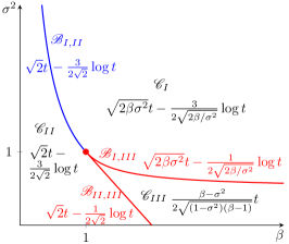
Figure 1: Phase diagram for the maximum of two type reducible BBM

Theorem 1.1 (Boundary between $\mathscr{C}_{II}$, $\mathscr{C}_{III}$).

Assume that $(\beta,\sigma^{2})\in\mathscr{B}_{II,III}$. Let

$$m^{2,3}_{t}:=\sqrt{2}t-\frac{1}{2\sqrt{2}}\log t.$$

Then for the constant $C=\frac{\alpha C_{\star}}{\sqrt{2}(1-\sigma^{2})}>0$, we have

$$\lim_{t\to\infty}\sum_{u\in N_{t}}\delta_{X_{u}(t)-m^{2,3}_{t}}=\lim_{t\to\infty}\sum_{u\in N^{2}_{t}}\delta_{X_{u}(t)-m^{2,3}_{t}}=\operatorname{DPPP}\left(\sqrt{2}CW_{\infty}^{(I)}(\sqrt{2})e^{-\sqrt{2}x}\mathop{}\!\mathrm{d}x,\mathfrak{D}^{\sqrt{2}}\right)\text{ in law}.$$

Theorem 1.1 confirms Conjecture 2.2 of Belloum and Mallein [13] with the constant before $\log t$ being corrected as $\frac{1}{2\sqrt{2}}$, and the random variable $\widetilde{Z}$ there taken to be $W^{(I)}_{\infty}(\sqrt{2})$.

Throughout this paper, we set

$$v:=\sqrt{2\beta\sigma^{2}}\ \text{ and }\ \theta:=\sqrt{{2\beta}/{\sigma^{2}}}.$$

Theorem 1.2 (Boundary between $\mathscr{C}_{I}$, $\mathscr{C}_{III}$).

Assume that $(\beta,\sigma^{2})\in\mathscr{B}_{I,III}$. Let

$$m^{1,3}_{t}:=vt-\frac{1}{2\theta}\log t.$$

Then we have

$$\lim_{t\to\infty}\sum_{u\in N_{t}}\delta_{X_{u}(t)-m^{1,3}_{t}}=\lim_{t\to\infty}\sum_{u\in N_{t}^{2}}\delta_{X_{u}(t)-m^{1,3}_{t}}=\mathrm{DPPP}\left(\theta CZ_{\infty}^{(I)}e^{-\theta x}\mathop{}\!\mathrm{d}x,\mathfrak{D}^{\theta}\right)\text{ in law}$$

with $C=\frac{\alpha\sigma C(\theta)}{\sqrt{2\pi}\beta(1-\sigma^{2})}$ (where $C(\theta)$ is defined in Lemma 2.4, (ii)).

Theorem 1.2 confirms Conjecture 2.1 of Belloum and Mallein [13] with the coefficient before $\log t$ being corrected as $\frac{1}{2\theta}$ and the decoration law $\widetilde{\mathfrak{D}}$ there taken to be $\mathfrak{D}^{\theta}$.

Theorem 1.3 (Boundary between $\mathscr{C}_{I}$, $\mathscr{C}_{II}$).

Assume that $(\beta,\sigma^{2})\in\mathscr{B}_{I,II}$. Let

$$m^{1,2}_{t}:=m_{t}=\sqrt{2}t-\frac{3}{2\sqrt{2}}\log t.$$

For some random variable $\bar{Z}_{\infty}$ (defined in Lemma 5.3), we have

$$\lim_{t\rightarrow\infty}\sum_{u\in N_{t}}\delta_{X_{u}(t)-m^{1,2}_{t}}=\lim_{t\rightarrow\infty}\sum_{u\in N_{t}^{2}}\delta_{X_{u}(t)-m^{1,2}_{t}}=\operatorname{DPPP}\left(\sqrt{2}C_{\star}\bar{Z}_{\infty}e^{-\sqrt{2}x}\mathop{}\!\mathrm{d}x,\mathfrak{D}^{\sqrt{2}}\right)\text{ in law.}$$

Remark 1.4.

Combining Theorems 1.1, 1.2, 1.3 and results in [13, 12], we can observe a double jump in the maximum $\max_{u\in N_{t}}X_{u}(t)$ when the parameters $(\beta,\sigma^{2})$ cross the boundary of anomalous spreading region $\mathscr{C}_{III}$. The leading order varies continuously but the logarithmic correction changes from $-\frac{3}{2\sqrt{2}}\log t$ to $-\frac{1}{2\sqrt{2}}\log t$ then to $0$; or from $-\frac{3}{2\theta}\log t$ to $-\frac{1}{2\theta}\log t$ then to $0$. See Figure 2. Such a phase transition reminds us of the study of time inhomogeneous BRW [32], in which a constant multiplying the logarithmic correction changes from $-\frac{1}{2}$ to $-\frac{3}{2}$ then to $-\frac{6}{2}$. Also in a more general setting of [32], phase transitions becomes a little bit more complex and a double jump can occur as well (see [44]). A more interesting problem is to make the logarithmic correction smoothly interpolates from $1$ to $6$, which is done for variable speed BBM in [23] (see also [37]). For two-type reducible BBMs, we ask a similar question as follows.

Question 1.

Can we let the parameters $(\beta_{t},\sigma^{2}_{t})$ depend on the time horizon $t$, in order that the logarithmic correction for the order of the maximum at time $t$ smoothly interpolates $-\frac{3}{2\sqrt{2}}\log t$ to $-\frac{1}{2\sqrt{2}}\log t$ then to $0$ or from $-\frac{3}{2\theta}\log t$ to $-\frac{1}{2\theta}\log t$ then to $0$?

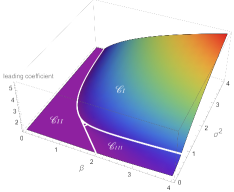
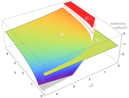
Figure 2: Coefficients for term $t$ and $\log t$ as function of $(\beta,\sigma^{2})$

Remark 1.5.

When $(\beta,\sigma^{2})\in\mathscr{B}_{I,II}$, the localization of paths of extremal particles is the same as the case $(\beta,\sigma^{2})\in\mathscr{C}_{II}$ (see Lemma 5.1). So when $(\beta,\sigma^{2})$ crosses the boundary between $\mathscr{C}_{I}$, $\mathscr{C}_{II}$, the maximum of the process only experience one jump: the subleading coefficient changes from $-\frac{3}{2\sqrt{2}}$ to $-\frac{3}{2\theta}$.

Remark 1.6.

Our results Theorems 1.1, 1.2, 1.3 can be strengthened as the joint convergence of the extremal processes and its maximum $(\mathcal{E}_{t},\max\mathcal{E}_{t})$ to DPPPs and its maximum $(\mathcal{E}_{\infty},\max\mathcal{E}_{\infty})$. Since by [14, Lemma 4.4], these assertions are both equivalent to convergence of Laplace functional $\mathbb{E}[e^{-\langle\phi,\mathcal{E}_{t}\rangle}]$ with certain test functions $\varphi\in\mathcal{T}$ introduced below.

Notation convention.

Let $\mathcal{T}$ be the set of functions $\varphi\in C_{b}^{+}(\mathbb{R})$ such that $\inf\mathrm{supp}(\varphi)>-\infty$ and for some $a\in\mathbb{R}$, $\varphi(x)\equiv$ some positive constant for all $x>a$. $\mathcal{T}$ will serve as test functions in the Laplace functional (see [14, Lemma 4.4]). For two quantities $f$ and $g$, we write $f\sim g$ if $\lim f/g=1$. We write $f\lesssim g$ if there exists a constant $C>0$ such that $f\leq Cg$. We write $f\lesssim_{\lambda}g$ to stress that the constant $C$ depends on parameter $\lambda$. We use the standard notation $\Theta(f)$ to denote a non-negative quantity such that there exists constant $c_{1},c_{2}>0$ such that $c_{1}f\leq\Theta(f)\leq c_{2}f$.

1.4 Heuristics

We restate the optimization problem introduced in [13, Section 2.1] (see also Biggins [16]). First, we introduce the following definition:

Definition 1.7.

If $u\in N^{2}_{t}$, we denote by $T_{u}$ the time at which the oldest ancestor of type $2$ of $u$ was born. We say $T_{u}$ is the type transformation time of $u$.

For $p\in[0,1]$, let $\mathcal{N}_{p,a,b}(t)$ be the expected number of type $2$ particles at time $t$ who has speed $a$ before time $T_{u}\approx pt$ and speed $b$ after time $pt$. Note that these particles are at level $[pa+(1-p)b]t$. First-moment computations yield that there are around $e^{\left(\beta-\frac{a^{2}}{2\sigma^{2}}\right)pt+o(t)}$ type $1$ particles at time $pt$ at level $apt$, and a type $2$ particle has probability $e^{\left(1-\frac{b^{2}}{2}\right)(1-p)t+o(t)}$ of having a descendant at level $b(1-p)t$ at time $(1-p)t$. Hence we get $\mathcal{N}_{p,a,b}(t)=\exp\left\{[(\beta-\frac{a^{2}}{2\sigma^{2}})p+(1-\frac{b^{2}}{2})(1-p)]t+o(t)\right\}$. In order to get the maximum, we just maximize $pa+(1-p)b$ among all the parameter $p,a,b$ such that $\left(\beta-\frac{a^{2}}{2\sigma^{2}}\right)p\geq 0$ and $\mathcal{N}_{p,a,b}(t)\geq 1$. This turns to the following optimization problem:

$$v^{*}=\max\left\{pa+(1-p)b:p\in[0,1],\left(\beta-\frac{a^{2}}{2\sigma^{2}}\right)p\geq 0,\left(\beta-\frac{a^{2}}{2\sigma^{2}}\right)p+(1-\frac{b^{2}}{2})(1-p)\geq 0\right\}.$$

Write $\left(p^{*},a^{*},b^{*}\right)$ for the maximizer of the problem above. If $\left(\beta,\sigma^{2}\right)\in\mathscr{C}_{I}$, then $p^{*}=1,a^{*}=v$, and $v^{*}=v$; if $\left(\beta,\sigma^{2}\right)\in\mathscr{C}_{II}$, then $p^{*}=0,b^{*}=\sqrt{2}$ and $v^{*}=\sqrt{2}$; if $\left(\beta,\sigma^{2}\right)\in\mathscr{C}_{III}$, then $p^{*}=\frac{\sigma^{2}+\beta-2}{2\left(1-\sigma^{2}\right)(\beta-1)}$, $b^{*}=\sqrt{2\frac{\beta-1}{1-\sigma^{2}}}$, $a^{*}=\sigma^{2}b^{*}$, and $v^{*}=\frac{\beta-\sigma^{2}}{\sqrt{2\left(1-\sigma^{2}\right)(\beta-1)}}$. Also if $(\beta,\sigma^{2})=(1,1)$, then $p^{*}$ can be arbitrary in $[0,1]$, $a^{*}=b^{*}=\sqrt{2}$ and $v^{*}=\sqrt{2}$.

When $(\beta,\sigma^{2})\in\mathscr{B}_{II,III}$, the maximizer $p^{*}=0$, $v^{*}=b^{*}=\sqrt{2}$, and $a^{*}$ can be arbitrary. Hence each individual $u\in N^{2}_{t}$ near the maximal position should satisfy $p^{*}=T_{u}/t\approx 0$. But now the order of $T_{u}$ really matters, and if $T_{u}\gg 1$, $a^{*}$ should be $\sqrt{2}\sigma^{2}$ predicted by the formula for the case $\mathscr{C}_{III}$. When $(\beta,\sigma^{2})\in\mathscr{B}_{I,III}$, the maximizer $p^{*}=1$, $v^{*}=a^{*}=v$, and $b^{*}$ can be arbitrary. We can deduce that each individual $u\in N^{2}_{t}$ near the maximal position satisfies $p^{*}=T_{u}/t\approx 1$. The order of $t-T_{u}$ is also important, and if $t-T_{u}\gg 1$, $b^{*}$ should be $\sqrt{2\beta/\sigma^{2}}$ predicted by the formula for the case $\mathscr{C}_{III}$. Similar problems occur when we consider the boundary $\mathscr{B}_{I,II}$. The following computations, based on a finer analysis, provide more insights for localization of paths of extremal particles.

The case $(\beta,\sigma^{2})\in\mathscr{B}_{II,III}$.

As the computation above, the expected number of particles of type $1$ at time $s=o(t)$ at level $\lambda s$ is roughly $e^{(\beta-\frac{\lambda^{2}}{2\sigma^{2}})s+O(\log t)}$. A typical particle of type $2$ has probability of $e^{-(2-\sqrt{2}\lambda)s-\frac{(\sqrt{2}-\lambda)^{2}}{2}\frac{s^{2}}{t-s}+O(\log t)}$ having a descendant at level $\sqrt{2}t-\lambda s$ at time $t-s$. Hence there are around

$$\exp\left\{\left[\beta-\frac{\lambda^{2}}{2\sigma^{2}}-(2-\sqrt{2}\lambda)\right]s-\frac{(\sqrt{2}-\lambda)^{2}}{2}\frac{s^{2}}{t-s}+O(\log t)\right\}$$ (1.6)

particles of type $2$ at level $\sqrt{2}t$ at time $t$. In order that the quantity in (1.6) is not zero as $t\to\infty$, first we have to ensure that $\beta-\frac{\lambda^{2}}{2\sigma^{2}}-(2-\sqrt{2}\lambda)=-\frac{1}{2\sigma^{2}}(\lambda-\sqrt{2}\sigma^{2})^{2}\geq 0$ (here we used $\beta+\sigma^{2}=2$), which forces $\lambda=\sqrt{2}\sigma^{2}$. Secondly we have to ensure that $\frac{s^{2}}{t-s}$ is bounded, i.e., $s=O(\sqrt{t})$. In other words, the extremal particle $u\in N^{2}_{t}$ should satisfy $T_{u}=O(\sqrt{t})$ and $X_{u}(T_{u})\approx\sqrt{2}\sigma^{2}T_{u}$.

The case $(\beta,\sigma^{2})\in\mathscr{B}_{I,III}$.

The expected number of type $1$ particles at time $s=t-o(t)$ at level $vs-a(t)$ (where $a(t)$ will be determined later) is roughly $e^{\theta a(t)-\frac{a(t)^{2}}{2s}+O(\log t)}$. A typical particle of type $2$ has the probability of $e^{-\left[(\frac{v^{2}}{2}-1)(t-s)+va(t)+\frac{a(t)^{2}}{2(t-s)}\right]+O(\log t)}$ having a descendant at level $v(t-s)+a(t)$ at time $t-s$. Hence there are around

$$\exp\left\{-\left[\left(\frac{v^{2}}{2}-1\right)(t-s)+\frac{a(t)^{2}}{2s}+\frac{a(t)^{2}}{2(t-s)}\right]+(\theta-v)a(t)+O(\log t)\right\}$$ (1.7)

particles of type $2$ at level $vt$ at time $t$. In order that the quantity in (1.7) is not zero as $t\to\infty$, using the prior knowledge $s\sim t$, first we have to ensure that $a(t)$ has the same order as $t-s$ or $\frac{a(t)^{2}}{t-s}$, and we get $a(t)=\Theta(t-s)$. We also need to ensure that $\frac{a(t)^{2}}{2s}=O(1)$, thus implies $a(t)=t-s=O(\sqrt{t})$. So, letting $a(t)=a\sqrt{t}$ and $t-s=\lambda\sqrt{t}$, we can rewrite (1.7) as

$$\exp\left\{\left(\theta a-\frac{(a+\lambda v)^{2}}{2\lambda}+\lambda\right)\sqrt{t}+O(\log t)\right\}.$$

We now have to ensure $\theta a-\frac{(a+\lambda v)^{2}}{2\lambda}+\lambda=-\frac{1}{2\lambda}[a-(\theta-v)\lambda]^{2}\geq 0$ (here we used $\frac{1}{\beta}+\frac{1}{\sigma^{2}}=2$). This forces $a=(\theta-v)\lambda$ and hence $a(t)=a\sqrt{t}=(\theta-v)(t-s)$. In other words, the extremal particle $u\in N^{2}_{t}$ should satisfy $T_{u}=t-\Theta(\sqrt{t})$ and $X_{u}(T_{u})\approx vT_{u}-(\theta-v)(t-T_{u})$.

The case $(\beta,\sigma^{2})\in\mathscr{B}_{I,II}$

We do the same computation as in the case $(\beta,\sigma^{2})\in\mathscr{B}_{I,III}$, and get (1.7). However, when $\beta\sigma^{2}=1$ and $\beta<1$, we have $v=\sqrt{2}$ and $\theta=\sqrt{2}\beta$, and then (1.7) becomes

$$\exp\left\{-\left[\sqrt{2}(1-\beta)a(t)+\frac{a(t)^{2}}{2s}+\frac{a(t)^{2}}{2(t-s)}\right]+O(\log t)\right\}.$$ (1.8)

In order that (1.8) tends to a nonzero limit, we need $a(t)=O(\log t)$. This is very different from the case $(\beta,\sigma^{2})=(1,1)$ in [12], for which case we can get $a(t)=O(\sqrt{t})$ (now $s$ is of order $t$). Now the simple first moment computations can not tell us more. However, we can still make a guess. Notice that the extremal particle $u\in N^{2}_{t}$ are also extremal (up to $O(\log t)$) at time $T_{u}$. This fact reminds us of the decreasing variances case in [32]: The maximum at time $t$ is the highest value among the descendants of the maximal particle at time $t/2$. So we guess that $\max_{u\in N_{t}}X_{u}(t)\approx\max_{T_{u}\in[0,t]}\{\sqrt{2}T_{u}-\frac{3}{2\theta}\log T_{u}+\sqrt{2}(t-T_{u})-\frac{3}{2\sqrt{2}}\log(t-T_{u})\}$. As $\theta<\sqrt{2}$, we should choose $T_{u}$ small. So we expect $T_{u}=O(1)$ and $\max_{u\in N_{t}}X_{u}(t)$ should be $\sqrt{2}t-\frac{3}{2\sqrt{2}}\log t$.

2 Preliminary results

2.1 Brownian motions estimates

We always use $\left\{(B_{t})_{t\geq 0};\mathbf{P}\right\}$ to denote a standard Brownian motion (BM) starting from the origin. Here is a useful upper bound for the probability that a Brownian bridge is below a line, see [26, Lemma 2] for a proof.

Lemma 2.1.

Consider a line segment with endpoints $(0,x_{1}),(t,x_{2})$ with $x_{1},x_{2}\geq 0$. We have

$$\mathbf{P}\left(B_{s}\leq\frac{s}{t}x_{2}+\frac{t-s}{t}x_{1},\,\forall s\in[0,t]\,\bigg{|}B_{t}=0\right)=1-e^{-\frac{2x_{1}x_{2}}{t}}\leq\frac{2x_{1}x_{2}}{t}.$$

As a corollary, we also have an estimate for the probability that a BM stays below a line and ends up in a finite interval. For all $K\geq 1$ and $y\geq 0$ we have

$$\mathbf{P}\left(B_{s}\leq K,s\leq t,B_{t}-K\in[-y-1,-y]\right)\leq C\frac{K(y+1)}{(1+t)^{3/2}}.$$ (2.1)

In fact, the desired probability is less than the product of $\mathbf{P}(B_{t}-K+y\in[-1,0])\leq\frac{1}{\sqrt{2\pi t}}$ and $\max_{z\in[0,1]}\mathbf{P}(B_{s}\leq K,\,\forall s\in[0,t]\,|B_{t}=K-y-z)\leq 2K(y+1)/t$ by Lemma 2.1.

Later in the proof of Lemma 4.1, we will use a slight modification of Lemma 2.1 as follows. For completeness, we give its proof in the appendix A.

Lemma 2.2.

Let $\widetilde{m}_{t}=vt-w_{t}$, where $w_{t}=\Theta(\log t)$. Assume that $\sigma^{2}\leq 1$. Fix $K\geq 0$ and $x\in\mathbb{{R}}$. Then for sufficiently large $t$ and $s\in[t-\sqrt{t}\log t,t]$,

$$\mathbf{P}\left(\sigma B_{r}\leq vr+K,\forall r\leq s|\sigma B_{s}+B_{t}-B_{s}=\widetilde{m}_{t}+x\right)\lesssim_{K,\beta,\sigma}\frac{t-s+w_{t}+|x|}{t}.$$ (2.2)

2.2 Branching Brownian motions estimates

We always use $\{(\mathsf{X}_{u}^{\beta,\sigma^{2}}(t):u\in\mathsf{N}_{t})_{t\geq 0},\mathsf{P}\}$ to denote a BBM starting from one particle at the origin with branching rate $\beta$ and diffusion coefficient $\sigma^{2}$. For the BBM, there is an upper envelope through which particles find it difficult to pass. In fact, letting $a_{t}=\frac{3}{2\theta}\log(t+1)$, for some constant $C>0$ and for all $t>0,K>0$,

$$\mathsf{P}\left(\exists s\leq t,u\in\mathsf{N}_{s}:\mathsf{X}^{\beta,\sigma^{2}}_{u}(s)\geq vs-a_{t}+a_{t-s}+K\right)\leq C(K+1)e^{-\theta K},$$ (2.3)

see [13, (6.1)] (or [45, Lemma 3.1]). In particular, we have

$$\mathsf{P}\left(\exists s\leq t,u\in\mathsf{N}_{s}:\mathsf{X}^{\beta,\sigma^{2}}_{u}(s)\geq vs+K\right)\leq C(K+1)e^{-\theta K}.$$ (2.4)

We collect several results for the standard BBM $(\mathsf{X}_{u}(t):u\in\mathsf{N}_{t})_{t\geq 0},$ (i.e., $\beta=\sigma^{2}=1$) that will be used frequently. Recall that $\mathsf{M}_{t}=\max_{u\in\mathsf{N}_{t}}\mathsf{X}_{u}(t)$. The following estimate of the upper tail of $\mathsf{M}_{t}$ was proved in [8, Corollary 10]

Lemma 2.3.

For $x>1$ and $t\geq t_{o}$ (for $t_{o}$ a numerical constant),

$$\mathsf{P}\left(\mathsf{M}_{t}\geq\sqrt{2}t-\frac{3}{2\sqrt{2}}\log t+x\right)\leq\rho\cdot x\cdot\exp\left(-\sqrt{2}x-\frac{x^{2}}{2t}+\frac{3}{2\sqrt{2}}x\frac{\log t}{t}\right)$$

for some constant $\rho>0$.

As a consequence of Lemma 2.3, we have

$$\mathsf{P}\left(\mathsf{M}_{t}\geq\sqrt{2}t-\frac{3}{2\sqrt{2}}\log t+x\right)\leq\rho\cdot x\exp\left(-\sqrt{2}x+1\right),$$ (2.5)

for all $x>1$ and $t>t_{0}$, since $-\frac{x^{2}}{2t}+\frac{3}{2\sqrt{2}}x\frac{\log t}{t}\leq 1$, for all $t>100$ and $x>1$.

The following estimates for the Laplace functionals of standard BBMs can be found in [12, Corollary 2.9] and [13, Corollary 2.9]. One can also obtain the same results from the large deviations probability $\mathsf{P}(\mathsf{M}_{t}>\rho t+x)$ with $\rho\geq\sqrt{2}$ and the conditioned convergence of the gap processes (1.3).

Lemma 2.4.

Let $\varphi\in\mathcal{T}$, $R>0$ and $\rho>\sqrt{2}$. Then the following assertions hold.

1. For $x\in[-R\sqrt{t},-\frac{1}{R}\sqrt{t}]$ uniformly

   $$1-\mathsf{E}\left(e^{-\sum_{u\in\mathsf{N}_{t}}\varphi\left(x+\mathsf{X}_{u}(t)-\sqrt{2}t\right)}\right)=\gamma_{\sqrt{2}}(\varphi)\frac{(-x)}{t^{3/2}}e^{\sqrt{2}x-\frac{x^{2}}{2t}}(1+o(1)),$$

   as $t\rightarrow\infty$, where $\gamma_{\sqrt{2}}(\varphi)=\displaystyle\sqrt{2}C_{\star}\int e^{-\sqrt{2}z}\left(1-\mathsf{E}\left(e^{-\langle\mathfrak{D}^{\sqrt{2}},\varphi(\cdot+z)\rangle}\right)\right)\mathop{}\!\mathrm{d}z$.

2. For $x\in[-R\sqrt{t},-\frac{1}{R}\sqrt{t}]$ uniformly

   $$1-\mathsf{E}\left(e^{-\sum_{u\in\mathsf{N}_{t}}\varphi\left(x+\mathsf{X}_{u}(t)-\rho t\right)}\right)=\gamma_{\rho}(\varphi)\frac{e^{\left(1-\rho^{2}/2\right)t}}{\sqrt{t}}e^{\rho x-\frac{x^{2}}{2t}}(1+o(1)),$$

   as $t\rightarrow\infty$, where $\gamma_{\rho}(\varphi)=\displaystyle\frac{C(\rho)}{\sqrt{2\pi}}\int e^{-\rho z}\left(1-\mathsf{E}(e^{-\left\langle\mathfrak{D}^{\rho},\varphi(\cdot+z)\right\rangle})\right)\mathop{}\!\mathrm{d}z$.

2.3 Choosing an individual according to Gibbs measure

For a standard BBM $\{(\mathsf{X}_{u}(t):u\in\mathsf{N}_{t}),\mathsf{P}\}$, it is well known that the additive martingale

$$\mathsf{W}_{t}(\eta)=\sum_{u\in\mathsf{N}_{t}}e^{\eta\mathsf{X}_{u}(t)-\left(\frac{\eta^{2}}{2}+1\right)t}$$

converges almost surely and in $L^{1}$ to a non-degenerate random variable $\mathsf{W}_{\infty}(\eta)$ when $\eta\in(0,\sqrt{2})$. And, when $\eta=\sqrt{2}$, the non-negative martingale $\mathsf{W}_{t}(\eta)$ converges to zero with probability one (see e.g. [38]). Conditioned on BBM at time $t$, we randomly choose a particle $u\in\mathsf{N}_{t}$ with probability $\frac{e^{\eta\mathsf{X}_{u}(t)}}{\sum_{u\in\mathsf{N}_{t}}e^{\eta\mathsf{X}_{u}(t)}}$, which is the so called Gibbs measure at inverse temperature $\eta$. Hence the additive martingale is the normalized partition function of the Gibbs measure.

Firstly we state a law of large number theorem for the particle chosen according to the Gibbs measure. This result is not new. Since we didn’t find a reference, we offer a simple proof in Section 6 for completeness.

Proposition 2.5.

Let $f$ be a bounded continuous function on $\mathbb{R}$. Suppose $\eta\in(0,\sqrt{2})$. Define

$$\mathsf{W}_{t}^{f}(\eta):=\sum_{u\in\mathsf{N}_{t}}f\left(\frac{\mathsf{X}_{u}(t)}{t}\right)e^{\eta\mathsf{X}_{u}(t)-\left(\frac{\eta^{2}}{2}+1\right)t}.$$

Then

$$\lim_{t\to\infty}\mathsf{W}_{t}^{f}(\eta)=f(\eta)\mathsf{W}_{\infty}(\eta)\ \text{ in }L^{1}(\mathsf{P}).$$

This law of large number holds since the Gibbs measure is supported on the particles at position around $\eta t$ for $\eta\in(0,\sqrt{2})$. One may further ask the fluctuations of $X_{u}(t)-\eta t$. Indeed a central limit theorem (CLT) holds (see [46, (1.14)]): for $\eta\in(0,\sqrt{2})$ and for each bounded continuous function $f$,

$$\lim_{t\rightarrow\infty}\sum_{u\in\mathsf{N}_{t}}f\left(\frac{\mathsf{X}_{u}(t)-\eta t}{\sqrt{t}}\right)e^{\eta\mathsf{X}_{u}(t)-t\left(\frac{\eta^{2}}{2}+1\right)}=W_{\infty}(\eta)\int_{\mathbb{R}}f(z)e^{-\frac{z^{2}}{2}}\frac{\mathop{}\!\mathrm{d}z}{\sqrt{2\pi}}\quad\mathsf{P}\text{-a.s.}$$

In the critical case $\eta=\sqrt{2}$, the limiting distribution in the CLT is no longer Gaussian, but the Rayleigh distribution $\mu(\mathop{}\!\mathrm{d}z)=ze^{-\frac{z^{2}}{2}}1_{\{z>0\}}\mathop{}\!\mathrm{d}z$. Madaule [41, Theorem 1.2] showed that for every bounded continuous function $F$,

$$\lim_{t\to\infty}\sqrt{t}\sum_{u\in\mathsf{N}_{t}}F\left(\frac{\sqrt{2}t-\mathsf{X}_{u}(t)}{\sqrt{t}}\right)e^{-\sqrt{2}(\sqrt{2}t-\mathsf{X}_{u}(t))}=\sqrt{\frac{2}{\pi}}\,\mathsf{Z}_{\infty}\langle F,\mu\rangle$$ (2.6)

in probability, where $\langle F,\mu\rangle:=\int_{0}^{\infty}F(z)\mu(\mathop{}\!\mathrm{d}z)$. In fact, Madaule’s result is a Donsker-type theorem for BRWs. A simple proof of (2.6) can be found in [43, Theorem B.1].

The following proposition gives a natural generalization of (2.6). We didn’t find such a result in the literature and to our knowledge, it is new.

Proposition 2.6.

Let $G$ be a non-negative bounded measurable function with compact support. Suppose $F_{t}(z)=G(\frac{z-r_{t}}{h_{t}})$, where $r_{t}$ and $h_{t}$ satisfy that for some $\epsilon>0$ and for large $t$, $t^{-\frac{1}{2}+\epsilon}\leq r_{t}\leq\bar{r}<\infty$ and $r_{t}+yh_{t}=\Theta(r_{t})$ uniformly for $y\in\mathrm{supp}(G)$. Define

$$\mathsf{W}^{F_{t}}_{t}(\sqrt{2}):=\sum_{u\in\mathsf{N}_{t}}F_{t}\left(\frac{\sqrt{2}t-\mathsf{X}_{u}(t)}{\sqrt{t}}\right)e^{-\sqrt{2}(\sqrt{2}t-\mathsf{X}_{u}(t))}.$$

Then we have

$$\lim_{t\to\infty}\frac{\sqrt{t}}{\langle F_{t},\mu\rangle}\,\mathsf{W}^{F_{t}}_{t}(\sqrt{2})=\sqrt{\frac{2}{\pi}}\mathsf{Z}_{\infty}\text{ in probability.}$$

Taking $r_{t}=\lambda$ and $h_{t}=t^{-1/4}$, and denoting $F_{t,\lambda}:=G((z-\lambda)t^{1/4})$, for any finite interval $I\subset(0,\infty)$ with strictly positive endpoints we have

$$\lim\limits_{t\to\infty}t^{3/4}\int_{I}\mathsf{W}^{F_{t,\lambda}}_{t}(\sqrt{2})\mathop{}\!\mathrm{d}\lambda=\sqrt{\frac{2}{\pi}}\,\mu(I)\int_{\mathbb{R}}G(y)\mathop{}\!\mathrm{d}y\,\mathsf{Z}_{\infty}\ \text{ in probability.}$$ (2.7)

Remark 2.7.

To make Proposition 2.6 easier to understand, we choose the function $G$ to be the indicator function $1_{[a,b]}$. Letting $h_{t}=1$ and $r_{t}=\lambda>0$, Proposition 2.6 gives the CLT (2.6):

$$\sqrt{t}\sum_{u\in\mathsf{N}_{t}}e^{-\sqrt{2}(\sqrt{2}t-\mathsf{X}_{u}(t))}1_{\{\sqrt{2}t-X_{u}(t)\in[(\lambda+a)\sqrt{t},(\lambda+b)\sqrt{t}]\}}=[1+o_{\mathsf{P}}(1)]\mu([\lambda+a,\lambda+b])\sqrt{\frac{2}{\pi}}\mathsf{Z}_{\infty}.$$

Letting $h_{t}=t^{-1/2}$ and $r_{t}=\lambda>0$, Proposition 2.6 yields that

$$\sqrt{t}\sum_{u\in\mathsf{N}_{t}}e^{-\sqrt{2}(\sqrt{2}t-\mathsf{X}_{u}(t))}1_{\{\sqrt{2}t-X_{u}(t)\in[\lambda\sqrt{t}+a,\lambda\sqrt{t}+b]\}}=[1+o_{\mathsf{P}}(1)]\frac{(b-a)}{\sqrt{t}}\lambda e^{-\frac{\lambda^{2}}{2}}\sqrt{\frac{2}{\pi}}\,\mathsf{Z}_{\infty}.$$

This can be thought of a local limit theorem (LLT) result for the position of a particle sampled according to the Gibbs measure with parameter $\eta=\sqrt{2}$. (See also [15, Theorem 4] for a LLT result in the case $\eta<\sqrt{2}$.) Letting $h_{t}=t^{-1/4}$ and $r_{t}=\lambda>0$, we get

$$\sqrt{t}\sum_{u\in\mathsf{N}_{t}}e^{-\sqrt{2}(\sqrt{2}t-\mathsf{X}_{u}(t))}1_{\{\sqrt{2}t-X_{u}(t)\in[\lambda\sqrt{t}+at^{1/4},\lambda\sqrt{t}+bt^{1/4}]\}}=[1+o_{\mathsf{P}}(1)]\frac{(b-a)}{t^{1/4}}\lambda e^{-\frac{\lambda^{2}}{2}}\sqrt{\frac{2}{\pi}}\,\mathsf{Z}_{\infty},$$

which can be regarded as a result between CLT and LLT.

Remark 2.8.

Formally, applying Proposition 2.6 to the function $zF_{t}(z)$, we have

$$\frac{1}{\langle F_{t}(z),\hat{\mu}\rangle}\sum_{u\in\mathsf{N}_{t}}F_{t}\left(\frac{\sqrt{2}t-\mathsf{X}_{u}(t)}{\sqrt{t}}\right)(\sqrt{2}t-X_{u}(t))e^{-\sqrt{2}(\sqrt{2}t-\mathsf{X}_{u}(t))}\to\mathsf{Z}_{\infty}\quad\text{in probability},$$

where $\hat{\mu}(\mathop{}\!\mathrm{d}z)=\sqrt{\frac{2}{\pi}}z^{2}e^{-z^{2}/2}1_{\{z>0\}}\mathop{}\!\mathrm{d}z$. A rigorous proof can be achieved by slightly modifying the proof of Proposition 2.6.

Remark 2.9.

In the proof of Proposition 2.6 (and proof of (2.6) [41, Theorem 1.2]), we use the powerful method developed in [4]. For the CLT case (i.e., $r_{t}=\Theta(1)=h_{t}$), it’s easy to get an $O(1)$ upper bound for the $2$nd moment $I_{2}(t)$ in $\eqref{eq-p-moment}$, and then easily show that $\Delta_{2}(t)$ in (6.14) is negligible. But this is not the case if $h_{t}=o(1)$ or $r_{t}=o(1)$. Especially we will apply Proposition 2.6 with $h_{t}=\Theta(t^{-1/4})$. To overcome this difficulty, we upper bound the $p$-th moment $I_{p}(t)$ in $\eqref{eq-p-moment}$ ($p\in(1,2)$ is carefully chosen) instead of the $2$nd moment. We also need to carefully choose parameters in the good event $G_{t}$ in (6.15). Combining these two things, we employ a bootstrap argument (6.16) to show that $\Delta_{p}(t)$ in (6.14) is negligible. Here our assumptions on $r_{t}$ and $h_{t}$ are near optimal, since for $h_{t}\leq r_{t}=o(\frac{\log t}{\sqrt{t}})$, (1.1) implies that $\frac{\sqrt{t}}{\langle F_{t},\mu\rangle}\,\mathsf{W}^{F_{t}}_{t}(\sqrt{2})\to 0$ in probability. Our arguments do fail if $\log t\leq r_{t}\sqrt{t}\ll t^{\epsilon}$ for all $\epsilon>0$.

2.4 Many-to-one lemmas for two-type BBMs

Let $\{(X_{u}(t),u\in N_{t}),\mathbb{P}\}$ be a two-type reducible BBM. Recall that for a type $2$ particle $u$, $T_{u}$ is the time at which the oldest ancestor of type $2$ of $u$ was born. Let $b_{u}$ be the time when $u$ was born. We write

$$\mathcal{B}=\left\{u\in\cup_{t\geq 0}\,N_{t}^{2},\quad T_{u}=b_{u}\right\}$$

for the set of particles of type $2$ that are born from a particle of type $1$. The following useful many-to-one lemmas were proved in [13, Proposition 4.1 and Corollary 4.3].

Lemma 2.10.

Let $f$ be a non-negative measurable function $f$. Then

1. $\displaystyle\mathbb{E}\bigg{(}\sum_{u\in N_{t}^{2}}f\left(\left(X_{u}(s),s\leq t\right),T_{u}\right)\bigg{)}=\alpha\int_{0}^{t}e^{\beta s+(t-s)}\mathbf{E}\bigg{(}f\left(\left(\sigma B_{u\wedge s}+\left(B_{u}-B_{u\wedge s}\right),u\leq t\right),s\right)\bigg{)}\mathop{}\!\mathrm{d}s$.

2. $\displaystyle\mathbb{E}\left(\sum_{u\in\mathcal{B}}f\left(X_{u}(s),s\leq T_{u}\right)\right)=\alpha\int_{0}^{\infty}e^{\beta t}\mathbf{E}\left(f\left(B_{s},s\leq t\right)\right)\mathop{}\!\mathrm{d}t$.

3. $\displaystyle\mathbb{E}\bigg{[}\exp\bigg{(}-\sum_{u\in\mathcal{B}}f\left(X_{u}(s),s\leq T_{u}\right)\bigg{)}\bigg{]}=\mathbb{E}\bigg{[}\exp\bigg{(}-\alpha\int_{0}^{\infty}\sum_{u\in N_{t}^{1}}1-e^{-f\left(X_{u}(s),s\leq t\right)}\mathop{}\!\mathrm{d}t\bigg{)}\bigg{]}$.

3 Boundary between $\mathscr{C}_{II}$ and $\mathscr{C}_{III}$

In this section we always assume that $(\beta,\sigma^{2})\in\mathscr{B}_{II,III}$, i.e., $\beta>1$, $\sigma^{2}=2-\beta<1$ and recall that $m^{2,3}_{t}:=\sqrt{2}t-\frac{1}{2\sqrt{2}}\log t$.

Lemma 3.1.

For any $A>0$, we have

$$\lim_{R\rightarrow\infty}\limsup_{t\rightarrow\infty}\mathbb{P}\left(\exists u\in N_{t}^{2}:T_{u}\notin[\frac{1}{R}\sqrt{t},R\sqrt{t}],X_{u}(t)\geq m^{2,3}_{t}-A\right)=0.$$

We are going to show Theorem 1.1, postponing the proof of Lemma 3.1 in the end of this section.

Proof of Theorem 1.1.

In this proof, we set $\widehat{\mathcal{E}}_{t}:=\sum_{u\in N_{t}^{2}}\delta_{X_{u}(t)-m^{2,3}_{t}}$, and for fixed $R>0$, let

$$\widehat{\mathcal{E}}_{t}^{R}:=\sum_{u\in N_{t}^{2}}1_{\left\{T_{u}\in[\frac{1}{R}\sqrt{t},R\sqrt{t}]\right\}}\delta_{X_{u}(t)-m^{2,3}_{t}}.$$

Thanks to Lemma 3.1, $\widehat{\mathcal{E}}_{t}^{R}$ is very close to $\widehat{\mathcal{E}}_{t}$. More precisely, for all $\varphi\in\mathcal{T}$, we have,

$$\left|\mathbb{E}\left(e^{-\left\langle\widehat{\mathcal{E}}_{t}^{R},\varphi\right\rangle}\right)-\mathbb{E}\left(e^{-\left\langle\widehat{\mathcal{E}}_{t},\varphi\right\rangle}\right)\right|\leq\mathbb{P}\left(\exists u\in N_{t}^{2}:X_{u}(t)\geq m^{2,3}_{t}-A,T_{u}\notin[\frac{1}{R}\sqrt{t},R\sqrt{t}]\right),$$

where $A$ is chosen such that $\mathrm{supp}(\varphi)\subset[-A,\infty)$. Thus applying Lemma 3.1 we have

$$\lim_{R\rightarrow\infty}\limsup_{t\rightarrow\infty}\left|\mathbb{E}\left(e^{-\left\langle\widehat{\mathcal{E}}_{t}^{R},\varphi\right\rangle}\right)-\mathbb{E}\left(e^{-\left\langle\widehat{\mathcal{E}_{t}},\varphi\right\rangle}\right)\right|=0.$$ (3.1)

Hence in order to study the asymptotic behavior of $\mathbb{E}\left(e^{-\left\langle\widehat{\mathcal{E}_{t}},\varphi\right\rangle}\right)$, we only need to study the convergence of $\widehat{\mathcal{E}}_{t}^{R}$ as $t$ and then $R$ goes to infinity.

Fix $R>0$ and $\varphi\in\mathcal{T}$. Observe that we can rewrite $\langle\widehat{\mathcal{E}}_{t}^{R},\varphi\rangle$ as

$$\sum\nolimits_{\begin{subarray}{c}u\in\mathcal{B}\\ T_{u}\in[\frac{1}{R}\sqrt{t},R\sqrt{t}]\end{subarray}}\sum\nolimits_{\begin{subarray}{c}u^{\prime}\in N_{t}^{2}\\ u^{\prime}\succcurlyeq u\end{subarray}}\varphi\left(X_{u^{\prime}}(t)-X_{u}(T_{u})-\sqrt{2}(t-T_{u})+X_{u}(T_{u})-\sqrt{2}T_{u}+\frac{1}{2\sqrt{2}}\log t\right),$$

where $u^{\prime}\succcurlyeq u$ means that $u^{\prime}$ is a descendant of $u$. Using the branching property first and then Lemma 2.10(iii), we have

$$\mathbb{E}\left(e^{-\left\langle\widehat{\mathcal{E}}_{t}^{R},\varphi\right\rangle}\right)=\mathbb{E}\bigg{(}\prod_{\begin{subarray}{c}u\in\mathcal{B}\\ T_{u}\in[\frac{1}{R}\sqrt{t},R\sqrt{t}]\end{subarray}}f\big{(}t-T_{u},X_{u}(T_{u})-\sqrt{2}T_{u}+\frac{1}{2\sqrt{2}}\log t\big{)}\bigg{)}$$

$$=\mathbb{E}\bigg{(}\exp\bigg{\{}-\alpha\int_{\frac{1}{R}\sqrt{t}}^{R\sqrt{t}}\sum_{u\in N_{s}^{1}}F\big{(}t-s,X_{u}(s)-\sqrt{2}s+\frac{1}{2\sqrt{2}}\log t\big{)}\mathop{}\!\mathrm{d}s\bigg{\}}\bigg{)},$$

where $F(r,x)=1-f(r,x)=1-\mathsf{E}\left(\exp\{-\sum_{u\in\mathsf{N}_{r}}\varphi(\mathsf{X}_{u}(r)-\sqrt{2}r+x)\}\right)$. Additionally, as the speed $v=\sqrt{2\beta\sigma^{2}}$ of the BBM of type $1$ is less than $\sqrt{2}$, we have, for all $s\in[\frac{1}{R}\sqrt{t},R\sqrt{t}]$ and $u\in N^{1}_{s}$, $\sqrt{2}s-X_{u}(s)=\Theta(s)$. Then applying part (i) of Lemma 2.4 we have, uniformly for $s\in[\frac{1}{R}\sqrt{t},R\sqrt{t}]$,

$$F\left(t-s,X_{u}(s)-\sqrt{2}s+\frac{1}{2\sqrt{2}}\log t\right)$$

$$=(1+o(1))\gamma_{\sqrt{2}}(\varphi)\frac{(\sqrt{2}s-X_{u}(s))}{t}e^{\sqrt{2}(X_{u}(s)-\sqrt{2}s)}e^{-\frac{(X_{u}(s)-\sqrt{2}s)^{2}}{2t}},$$

as $t\rightarrow\infty$, where the $o(1)$ term is deterministic. Thus $\mathbb{E}\left(e^{-\left\langle\widehat{\mathcal{E}}_{t}^{R},\varphi\right\rangle}\right)$

$$=\mathbb{E}\bigg{(}\exp\bigg{\{}-(1+o(1))\alpha\gamma_{\sqrt{2}}(\varphi)\times\int_{\frac{1}{R}\sqrt{t}}^{R\sqrt{t}}\sum_{u\in N_{s}^{1}}\frac{(\sqrt{2}s-X_{u}(s))}{t}e^{\sqrt{2}(X_{u}(s)-\sqrt{2}s)}e^{-\frac{(X_{u}(s)-\sqrt{2}s)^{2}}{2t}}\mathop{}\!\mathrm{d}s\bigg{\}}\bigg{)}$$

$$=\mathbb{E}\bigg{(}\exp\bigg{\{}-(1+o(1))\alpha\gamma_{\sqrt{2}}(\varphi)\int_{\frac{1}{R}}^{R}\mathcal{W}(\lambda,\lambda\sqrt{t})\mathop{}\!\mathrm{d}\lambda\bigg{\}}\bigg{)},$$ (3.2)

where

$$\mathcal{W}(\lambda,t):=\sum_{u\in N^{1}_{t}}\lambda\left(\sqrt{2}-\tfrac{X_{u}(t)}{t}\right)e^{-\frac{\lambda^{2}}{2}(\sqrt{2}-\frac{X_{u}(t)}{t})^{2}}e^{\sqrt{2}(X_{u}(t)-\sqrt{2}t)}.$$

Recall that $(\{X_{u}(t)\}_{u\in N^{1}_{t}},\mathbb{P})$ has the same distribution as $(\{\frac{\sigma}{\sqrt{\beta}}\mathsf{X}_{u}(\beta t)\}_{u\in\mathsf{N}_{\beta t}},\mathsf{P})$. Applying Proposition 2.5, we have, for each $\lambda>0$,

$$\lim_{t\to\infty}\mathcal{W}(\lambda,t)=\sqrt{2}\lambda(1-\sigma^{2})e^{-(1-\sigma^{2})^{2}\lambda^{2}}W_{\infty}^{(I)}(\sqrt{2})\ \text{ in }L^{1}(\mathbb{P}),$$

Then by the dominated convergence theorem, we have, as $t\to\infty$,

$$\mathbb{E}\left|\int_{1/R}^{R}\mathcal{W}(\lambda,\lambda\sqrt{t})\mathop{}\!\mathrm{d}\lambda-\sqrt{2}\int_{1/R}^{R}\lambda(1-\sigma^{2})e^{-(1-\sigma^{2})^{2}\lambda^{2}}W_{\infty}^{(I)}(\sqrt{2})\mathop{}\!\mathrm{d}\lambda\right|$$

$$\leq\int_{1/R}^{R}\mathbb{E}\left|\mathcal{W}(\lambda,\lambda\sqrt{t})-\sqrt{2}\lambda(1-\sigma^{2})e^{-(1-\sigma^{2})^{2}\lambda^{2}}W_{\infty}^{(I)}(\sqrt{2})\right|\mathop{}\!\mathrm{d}\lambda\to 0.$$

Here dominated functions exist since $\mathbb{E}[\mathcal{W}(\lambda,\lambda\sqrt{t})]$, $\mathbb{E}[\sqrt{2}\lambda(1-\sigma^{2})e^{-(1-\sigma^{2})^{2}\lambda^{2}}W_{\infty}^{(I)}(\sqrt{2})]$ are both bouned by $\max_{x\geq 0}xe^{-x^{2}/2}$. Letting $t\to\infty$ in (3.2), we have

$$\lim_{t\to\infty}\mathbb{E}\left(e^{-\left\langle\widehat{\mathcal{E}}_{t}^{R},\varphi\right\rangle}\right)=\mathbb{E}\bigg{(}\exp\bigg{\{}-\alpha\gamma_{\sqrt{2}}(\varphi)W_{\infty}^{(I)}(\sqrt{2})\int_{\frac{1}{R}}^{R}\sqrt{2}\lambda(1-\sigma^{2})e^{-(1-\sigma^{2})^{2}\lambda^{2}}\mathop{}\!\mathrm{d}\lambda\bigg{\}}\bigg{)}.$$

Then letting $R\to\infty$, combining (3.1), we obtain

$$\lim_{t\to\infty}\mathbb{E}\left(e^{-\left\langle\widehat{\mathcal{E}}_{t},\varphi\right\rangle}\right)=\lim_{R\to\infty}\lim_{t\to\infty}\mathbb{E}\left(e^{-\left\langle\widehat{\mathcal{E}}_{t}^{R},\varphi\right\rangle}\right)=\mathbb{E}\bigg{(}\exp\bigg{\{}-\frac{\alpha W_{\infty}^{(I)}(\sqrt{2})}{\sqrt{2}(1-\sigma^{2})}\gamma_{\sqrt{2}}(\varphi)\bigg{\}}\bigg{)},$$

which is the Laplace functional of $\operatorname{DPPP}\left(\frac{\alpha C_{\star}}{\sqrt{2}(1-\sigma^{2})}\sqrt{2}W_{\infty}^{(I)}(\sqrt{2})e^{-\sqrt{2}x}\mathop{}\!\mathrm{d}x,\mathfrak{D}^{\sqrt{2}}\right)$. Using [14, Lemma 4.4], we complete the proof of Theorem 1.1. ∎

Now it suffices to show Lemma 3.1. First we give prior estimates for the type transformation times $T_{u}$ for particles $u\in N^{2}_{t}$ with positions higher than $m^{2.3}_{t}$.

Lemma 3.2.

For any $A>0$ we have

$$\limsup_{t\rightarrow\infty}\mathbb{P}\left(\exists u\in N_{t}^{2}:T_{u}>\sqrt{t}\log t,X_{u}(t)\geq m^{2,3}_{t}-A\right)=0.$$ (3.3)

Proof.

Let $Y^{A}_{t}:=\sum_{u\in N^{2}_{t}}1_{\{T_{u}>\sqrt{t}\log t,X_{u}(t)\geq m^{2,3}_{t}-A\}}$. By Markov’s inequality, the probability in (3.3) is bounded by $\mathbb{E}\left(Y^{A}_{t}\right)$. It suffices to show that $\mathbb{E}\left(Y^{A}_{t}\right)\to 0$ as $t\to\infty$.

Using Lemma 2.10(i) and then the tail probability of Gaussian random variable ($\int^{\infty}_{x}e^{-y^{2}/2}\mathop{}\!\mathrm{d}y\leq\frac{1}{x}e^{-x^{2}/2}$ for $x>0$), we have

$$\mathbb{E}\left(Y^{A}_{t}\right) =\alpha\int_{\sqrt{t}\log t}^{t}e^{\beta s+t-s}\mathbf{P}\left(\sigma B_{s}+\left(B_{t}-B_{s}\right)\geq m^{2,3}_{t}-A\right)\mathop{}\!\mathrm{d}s$$

$$\lesssim_{\alpha}\int_{\sqrt{t}\log t}^{t}e^{\beta s+(t-s)}\frac{\sqrt{\sigma^{2}s+t-s}}{m^{2,3}_{t}-A}e^{-\frac{(m^{2,3}_{t}-A)^{2}}{2\left(\sigma^{2}s+t-s\right)}}\mathop{}\!\mathrm{d}s$$

$$\lesssim_{A,\alpha,\beta,\sigma^{2}}t^{-1/2}\int_{\sqrt{t}\log t}^{t}e^{\beta s+(t-s)-\frac{t^{2}}{\left(\sigma^{2}s+t-s\right)}}e^{\frac{t\log t}{2\left(\sigma^{2}s+t-s\right)}}\mathop{}\!\mathrm{d}s.$$

Set $\varphi:u\mapsto\beta u+(1-u)-\frac{1}{\left(\sigma^{2}u+1-u\right)}$. Making a change of variable $s=ut$, we have

$$\mathbb{E}\left(Y^{A}_{t}\right)\lesssim t^{1/2}\int_{\frac{\log t}{\sqrt{t}}}^{1}\exp\left\{t\varphi(u)+\frac{\log t}{2\left(\sigma^{2}u+1-u\right)}\right\}\mathop{}\!\mathrm{d}u\leq t^{\frac{1}{2}+\frac{1}{2\sigma^{2}}}\int_{\frac{\log t}{\sqrt{t}}}^{1}e^{t\varphi(u)}\mathop{}\!\mathrm{d}u.$$

Since $\varphi^{\prime}(u)=\beta-1-\frac{1-\sigma^{2}}{\left(\sigma^{2}u+1-u\right)^{2}}<0$ and $\varphi^{\prime\prime}(u)=-\frac{2\left(1-\sigma^{2}\right)^{2}}{\left(\sigma^{2}u+1-u\right)^{3}}<0$, $\varphi$ is concave, and takes maximum $\varphi(0)=0$ at point $u=0$. By Taylor’s expansion, there exists a constant $\delta>0$ (depending only on $\sigma^{2}$) such that $\varphi(u)\leq-\delta u^{2}$ for all $u\in[0,1]$. Thus

$$\mathbb{E}\left(Y^{A}_{t}\right)\lesssim t^{\frac{1}{2}+\frac{1}{2\sigma^{2}}}\int_{\frac{\log t}{\sqrt{t}}}^{1}e^{-\delta u^{2}t}\mathop{}\!\mathrm{d}u\leq t^{\frac{1}{2\sigma^{2}}}\int_{\log t}^{\infty}e^{-\delta z^{2}}\mathop{}\!\mathrm{d}z\overset{t\to\infty}{\longrightarrow}0,$$

which gives the desired result. ∎

Proof of Lemma 3.1.

Fix $A,K,t\geq 0$ and $R>1$. Set $I^{R}_{t}:=\left[0,\frac{1}{R}\sqrt{t}\right)\cup\left(R\sqrt{t},\sqrt{t}\log t\right]$, and

$$Y_{t}(A,R,K)=\sum_{u\in\mathcal{B}}1_{\left\{T_{u}\in I^{R}_{t}\right\}}1_{\{|X_{u}(T_{u})|\leq vT_{u}+K\}}1_{\left\{M_{t}^{u}\geq m^{2,3}_{t}-A\right\}},$$

where $M_{t}^{u}$ is the maximal position of the descendants at time $t$ of the individual $u$. In other words, $Y_{t}(A,R,K)$ is the number of type $2$ particles that are born from a type $1$ particle during the time interval $I^{R}_{t}$ and have a descendant at time $t$ above $m^{2,3}_{t}-A$. By Markov’s inequality,

$$\mathbb{P}\left(\exists u\in N_{t}^{2}:T_{u}\notin\left[\frac{1}{R}\sqrt{t},R\sqrt{t}\right],X_{u}(t)\geq m^{2,3}_{t}-A\right)$$

$$\leq \mathbb{P}\left(\exists s\leq t,u\in N^{1}_{s}:|X_{u}(s)|\geq vs+K\right)$$

$$+\mathbb{P}\left(\exists u\in N_{t}^{2}:T_{u}\geq\sqrt{t}\log t,X_{u}(t)\geq m^{2,3}_{t}-A\right)+\mathbb{E}\left(Y_{t}(A,R,K)\right).$$

By (2.4) and Lemma 3.2, it suffices to show that $\lim\limits_{R\to\infty}\limsup\limits_{t\rightarrow\infty}\mathbb{E}\left(Y_{t}(A,R,K)\right)=0$.

Let $F_{t}(r,x):=\mathsf{P}(x+\mathsf{M}_{r}\geq m^{2,3}_{t}-A)$, where $\mathsf{M}_{r}=\max\limits_{u\in\mathsf{N}_{r}}\mathsf{X}_{u}(r)$. Applying the branching property and Lemma 2.10(i), we have

$$\mathbb{E}\left(Y_{t}(A,R,K)\right)=\mathbb{E}\left(\sum_{u\in\mathcal{B}}1_{\left\{T_{u}\in I^{R}_{t}\right\}}1_{\{|X_{u}(T_{u})|\leq vT_{u}+K\}}F_{t}\left(t-T_{u},X_{u}(T_{u})\right)\right)$$ (3.4)

$$=\alpha\int_{I^{R}_{t}}e^{\beta s}\mathbf{E}\left(F_{t}\left(t-s,\sigma B_{s}\right)1_{\{|\sigma B_{s}|\leq vs+K\}}\right)\mathop{}\!\mathrm{d}s$$

$$=\alpha\int_{I^{R}_{t}}\mathbf{E}\left(e^{-\theta\sigma B_{s}}F_{t}\left(t-s,\sigma B_{s}+vs\right)\right)1_{\{-2vs-K\leq\sigma B_{s}\leq+K\}}\mathop{}\!\mathrm{d}s,$$

where in the last equality we replaced $\sigma B_{s}$ by $\sigma B_{s}+vs$ by Girsanov’s theorem. Moreover, since $\log t-\log(t-s)=o(1)$ for $s\leq\sqrt{t}\log t$, we have for large $t$,

$$F_{t}(t-s,vs+z)=\mathsf{P}\left(\mathsf{M}_{t-s}\geq\sqrt{2}t-\frac{1}{2\sqrt{2}}\log t-A-vs-z\right)$$

$$\leq\mathsf{P}\left(\mathsf{M}_{t-s}\geq\sqrt{2}(t-s)-\frac{3}{2\sqrt{2}}\log(t-s)+(\sqrt{2}-v)s+\frac{1}{\sqrt{2}}\log t-z-2A\right).$$

For $z\in[-2vs-K,K]$ and $s\leq\sqrt{t}\log t$, we have $1<(\sqrt{2}-v)s+\frac{1}{\sqrt{2}}\log t-z-2A\lesssim\sqrt{t}\log t$ for large $t$. Applying Lemma 2.3, we have

$$F(t-s,vs+z)\lesssim_{A,\beta,\sigma^{2}}\frac{s+\log t+|z|}{t}e^{-\sqrt{2}(\sqrt{2}-v)s+\sqrt{2}z}e^{-\frac{(\sqrt{2}-v)^{2}s^{2}}{2t}},$$ (3.5)

where we used the fact that $-\frac{1}{2(t-s)}\big{[}(\sqrt{2}-v)s+\frac{1}{\sqrt{2}}\log t-z-2A\big{]}^{2}\leq-\frac{(\sqrt{2}-v)^{2}s^{2}}{2t}$ for large $t$. Replacing $z$ by $\sigma B_{s}$ in (3.5) and then substituting (3.5) into (3.4), we obtain

$$\mathbb{E}\left(Y_{t}(A,R,K)\right) \lesssim_{\alpha,A,\beta,\sigma^{2}}\int_{I^{R}_{t}}\mathbf{E}\left(\frac{s+\log t+|\sigma B_{s}|}{t}e^{-(\theta-\sqrt{2})\sigma B_{s}-\sqrt{2}(\sqrt{2}-v)s}\right)e^{-\frac{(\sqrt{2}-v)^{2}s^{2}}{2t}}\mathop{}\!\mathrm{d}s$$

$$=\int_{I^{R}_{t}}\mathbf{E}\left(\frac{s+\log t+|\sigma B_{s}-(\theta-\sqrt{2})\sigma^{2}s|}{t}\right)e^{-\frac{(\sqrt{2}-v)^{2}s^{2}}{2t}}\mathop{}\!\mathrm{d}s$$

$$\lesssim\int_{[0,\frac{1}{R})\cup(R,\log t]}\left(\lambda+\frac{\log t+\mathbf{E}|B_{\lambda\sqrt{t}}|}{\sqrt{t}}\right)e^{-\frac{(\sqrt{2}-v)^{2}\lambda^{2}}{2}}\mathop{}\!\mathrm{d}\lambda,$$

where in the equality we used the Girsanov’s theorem and the fact that $\frac{1}{2}(\theta-\sqrt{2})^{2}\sigma^{2}=\sqrt{2}(\sqrt{2}-v)$ when $\beta+\sigma^{2}=2$, and in the last $\lesssim$ we made a change of variable $s=\sqrt{t}\lambda$. Then the desired results follows from a simple computation. ∎

4 Boundary between $\mathscr{C}_{I}$ and $\mathscr{C}_{III}$

In this section we always assume that $(\beta,\sigma^{2})\in\mathscr{B}_{I,III}$, i.e., $\beta>1$, $\frac{1}{\beta}+\frac{1}{\sigma^{2}}=2$. Recall that $m^{1,3}_{t}:=vt-\frac{1}{2\theta}\log t$, where $v=\sqrt{2\beta\sigma^{2}}$ and $\theta=\sqrt{2\beta/\sigma^{2}}$.

Firstly, we describe the paths of extremal particles. It turns out that for a type $2$ particle $u\in N^{2}_{t}$ above level $m^{1,3}_{t}$ at time $t$, it’s type transformation time $T_{u}$ should be $s=t-\Theta(\sqrt{t})$, and it’s position $x$ at time $s$ should belong to the set

$$\Gamma_{s,t}^{R}:=\left\{x:|\delta(x;s,t)|\leq R\sqrt{t-s}\right\}\,,\text{ where }\ \delta(x;s,t):=x-vs+(\theta-v)(t-s).$$

Lemma 4.1.

For any $A>0$, we have

$$\lim_{R\rightarrow\infty}\limsup_{t\rightarrow\infty}\mathbb{P}\left(\exists u\in N_{t}^{2}:t-T_{u}\notin[\frac{1}{R}\sqrt{t},R\sqrt{t}],X_{u}(t)\geq m^{1,3}_{t}-A\right)=0,$$ (4.1)

and

$$\lim_{R\rightarrow\infty}\limsup_{t\rightarrow\infty}\mathbb{P}\left(\exists u\in N_{t}^{2}:X_{u}(t)\geq m^{1,3}_{t}-A,X_{u}(T_{u})\notin\Gamma^{R}_{T_{u},t}\right)=0.$$ (4.2)

We will postpone the proof of Lemma 4.1 to the end of this section and show Theorem 1.2 first. For simplicity, let $\Omega^{R}_{t}=\{(s,x):t-s\in[\frac{1}{R}\sqrt{t},R\sqrt{t}],x\in\Gamma_{s,t}^{R}\}$.

Proof of Theorem 1.2.

In this proof, we set $\widehat{\mathcal{E}}_{t}:=\sum_{u\in N_{t}^{2}}\delta_{X_{u}(t)-m^{1,3}_{t}}$, and for $R>0$,

$$\widehat{\mathcal{E}}_{t}^{R}:=\sum_{u\in N_{t}^{2}}1_{\left\{(T_{u},X_{u}(T_{u}))\in\Omega^{R}_{t}\right\}}\delta_{X_{u}(t)-m^{1,3}_{t}}.$$

Take $A>0$ satisfying $\mathrm{supp}(\varphi)\subset[-A,\infty)$. For all $\varphi\in\mathcal{T}$, we have

$$\left|\mathbb{E}\left(e^{-\left\langle\widehat{\mathcal{E}}_{t}^{R},\varphi\right\rangle}\right)-\mathbb{E}\left(e^{-\left\langle\widehat{\mathcal{E}}_{t},\varphi\right\rangle}\right)\right|\leq\mathbb{P}\left(\exists u\in N_{t}^{2},X_{u}(t)\geq m^{1,3}_{t}-A,(T_{u},X_{u}(T_{u}))\notin\Omega^{R}_{t}\right).$$

Thus by Lemma 4.1 we have

$$\lim_{R\rightarrow\infty}\limsup_{t\rightarrow\infty}\left|\mathbb{E}\left(e^{-\left\langle\widehat{\mathcal{E}}_{t}^{R},\varphi\right\rangle}\right)-\mathbb{E}\left(e^{-\left\langle\widehat{\mathcal{E}_{t}},\varphi\right\rangle}\right)\right|=0.$$ (4.3)

We now show the convergence of $\widehat{\mathcal{E}}_{t}^{R}$ first as $t$ and then $R$ goes to $\infty$. Recall that $u^{\prime}\succcurlyeq u$ means that $u^{\prime}$ is a descendant of $u$. We rewrite $\langle\widehat{\mathcal{E}}_{t}^{R},\varphi\rangle$ as

$$\sum\nolimits_{\begin{subarray}{c}u\in\mathcal{B}\\ (T_{u},X_{u}(T_{u}))\in\Omega^{R}_{t}\end{subarray}}\sum\nolimits_{\begin{subarray}{c}u^{\prime}\in N_{t}^{2}\\ u^{\prime}\succcurlyeq u\end{subarray}}\ \varphi(X_{u^{\prime}}(t)-X_{u}(T_{u})-\theta(t-T_{u})+\delta(X_{u}(T_{u});T_{u},t)+\frac{1}{2\theta}\log t).$$

Let $f(r,x):=\mathsf{E}\left(\exp\{-\sum_{u\in\mathsf{N}_{r}}\varphi(\mathsf{X}_{u}(r)-\theta r+x)\}\right)$ and $F:=1-f$. Using the branching property first and then applying Lemma 2.10(iii), we have

$$\mathbb{E}\left(e^{-\left\langle\widehat{\mathcal{E}}_{t}^{R},\varphi\right\rangle}\right)=\mathbb{E}\bigg{[}\prod\nolimits_{\begin{subarray}{c}u\in\mathcal{B}\\ (T_{u},X_{u}(T_{u}))\in\Omega^{R}_{t}\end{subarray}}f\bigg{(}t-T_{u},\delta(X_{u}(T_{u});T_{u},t)+\frac{1}{2\theta}\log t\bigg{)}\bigg{]}$$

$$=\mathbb{E}\bigg{(}\exp\bigg{\{}-\alpha\int^{t-\frac{1}{R}\sqrt{t}}_{t-R\sqrt{t}}\sum_{u\in N_{s}^{1}}F\bigg{(}t-s,\delta(X_{u}(s);s,t)+\frac{1}{2\theta}\log t\bigg{)}1_{\{X_{u}(s)\in\Gamma_{s,t}^{R}\}}\mathop{}\!\mathrm{d}s\bigg{\}}\bigg{)}.$$

Additionally, by Lemma 2.4 (ii), uniformly in $s\in t-[\frac{1}{R}\sqrt{t},R\sqrt{t}]$ and in $X_{u}(s)\in\Gamma^{R}_{s,t}$, the function $F\left(t-s,\delta(X_{u}(s);s,t)+\frac{1}{2\theta}\log t\right)$

$$\sim\gamma_{\theta}(\varphi)\frac{e^{-(\frac{\theta^{2}}{2}-1)(t-s)}}{\sqrt{t-s}}e^{\theta[X_{u}(s)-v(s)+(\theta-v)(t-s)+\frac{1}{2\theta}\log t]}e^{-\frac{[X_{u}(s)-v(s)+(\theta-v)(t-s)+\frac{1}{2\theta}\log t]^{2}}{2(t-s)}}$$

$$\sim\gamma_{\theta}(\varphi)\sqrt{\frac{t}{t-s}}e^{\theta[X_{u}(s)-v(s)]}e^{-\frac{[X_{u}(s)-v(s)+(\theta-v)(t-s)]^{2}}{2(t-s)}},\ \text{ as }t\to\infty$$

where in the last “$\sim$” we used the fact that $\theta^{2}-\theta v-(\frac{\theta^{2}}{2}-1)=\frac{\beta}{\sigma^{2}}-2\beta+1=0$. Therefore, by making a change of variable $r=t-s$, we have $\mathbb{E}\left(e^{-\left\langle\widehat{\mathcal{E}}_{t}^{R},\varphi\right\rangle}\right)$

$$=\mathbb{E}\bigg{(}\exp\bigg{\{}-(1+o(1))\alpha\gamma_{\theta}(\varphi)\int_{\frac{1}{R}\sqrt{t}}^{R\sqrt{t}}\sqrt{\frac{t}{r}}\sum_{\begin{subarray}{c}u\in N_{s}^{1}\\ X_{u}(t-r)\in\Gamma_{t-r,t}^{R}\end{subarray}}e^{\theta[X_{u}(t-r)-v(t-r)]}e^{-\frac{[X_{u}(t-r)-v(t-r)+(\theta-v)r]^{2}}{2r}}\mathop{}\!\mathrm{d}r\bigg{\}}\bigg{)}$$

$$=\mathbb{E}\bigg{(}\exp\bigg{\{}-(1+o(1))\alpha\gamma_{\theta}(\varphi)\int_{\frac{1}{R}}^{R}\frac{t}{\sqrt{r_{\lambda,t}}}\mathcal{W}^{G}\left(t-r_{\lambda,t},r_{\lambda,t}\right)\mathop{}\!\mathrm{d}\lambda\bigg{\}}\bigg{)},$$ (4.4)

where in (4.4) we substitute $r$ by $r_{\lambda,t}=\lambda\sqrt{t}$, and

$$\mathcal{W}^{G}(t,r):=\sum_{u\in N^{1}_{t}}e^{-\theta[vt-X_{u}(t)]}G\left(\frac{vt-X_{u}(t)-(\theta-v)r}{\sqrt{r}}\right)\,,\ G(x)=e^{-\frac{x^{2}}{2}}1_{\{|x|\leq R\}}.$$

Recall that $(\{X_{u}(t)\}_{u\in N^{1}_{t}},\mathbb{P})$ has the same distribution as $(\{\frac{\sigma}{\sqrt{\beta}}\mathsf{X}_{u}(\beta t)\}_{u\in\mathsf{N}_{\beta t}},\mathsf{P})$. Applying Proposition 2.6, we have, for fixed $\lambda>0$ and $r_{\lambda,t}=\lambda\sqrt{t}$,

$$\lim_{t\to\infty}\frac{t}{\sqrt{r_{\lambda,t}}}\mathcal{W}^{G}(t-r_{\lambda,t},r_{\lambda,t})=Z_{\infty}^{(I)}\sqrt{\frac{2}{\pi}}\frac{(\theta-v)}{\sigma^{3}}\lambda\,e^{-\frac{(\theta-v)^{2}}{2\sigma^{2}}\lambda^{2}}\int_{\mathbb{R}}e^{-\frac{x^{2}}{2}}1_{\{|x|\leq R\}}\mathop{}\!\mathrm{d}y$$

in probability, and the integral of $\frac{t}{\sqrt{r_{\lambda,t}}}\mathcal{W}^{G}(t-r_{\lambda,t},r_{\lambda,t})$ with respect to $\lambda$ over the interval $[1/R,R]$ converges in probability to the integral of right hand side. By (4.4) and the dominated convergence theorem, we have $\lim\limits_{t\to\infty}\mathbb{E}\left(e^{-\left\langle\widehat{\mathcal{E}}_{t}^{R},\varphi\right\rangle}\right)=$

$$\mathbb{E}\bigg{(}\exp\bigg{\{}-\alpha\gamma_{\theta}(\varphi)Z_{\infty}^{(I)}\sqrt{\frac{2}{\pi}}\int_{\frac{1}{R}}^{R}\frac{(\theta-v)\lambda}{\sigma^{3}}e^{-\frac{(\theta-v)^{2}}{2\sigma^{2}}\lambda^{2}}\mathop{}\!\mathrm{d}\lambda\int_{\mathbb{R}}e^{-\frac{x^{2}}{2}}1_{\{|x|\leq R\}}\mathop{}\!\mathrm{d}y\bigg{\}}\bigg{)}.$$

Letting $R\to\infty$, combining (4.3), we have

$$\lim_{t\to\infty}\mathbb{E}\left(e^{-\left\langle\widehat{\mathcal{E}}_{t},\varphi\right\rangle}\right)=\lim_{R\to\infty}\lim_{t\to\infty}\mathbb{E}\left(e^{-\left\langle\widehat{\mathcal{E}}_{t}^{R},\varphi\right\rangle}\right)=\mathbb{E}\bigg{(}\exp\big{\{}-\gamma_{\theta}(\varphi)Z^{(I)}_{\infty}\frac{\alpha}{\sigma(\theta-v)}\big{\}}\bigg{)},$$

which is the Laplace functional of $\mathrm{DPPP}\left(\frac{\alpha\sigma C(\theta)}{\sqrt{2\pi}\beta(1-\sigma^{2})}\theta Z_{\infty}^{(I)}e^{-\theta x}\mathop{}\!\mathrm{d}x,\mathfrak{D}^{\theta}\right)$. Using [14, Lemma 4.4], we complete the proof of Theorem 1.2. ∎

Before proving Lemma 4.1, we show a weaker result first.

Lemma 4.2.

For any $A>0$ we have

$$\limsup_{t\rightarrow\infty}\mathbb{P}\left(\exists u\in N_{t}^{2}:T_{u}\leq t-\sqrt{t}\log t,X_{u}(t)\geq m^{1,3}_{t}-A\right)=0.$$

Proof.

For $A>0$, we compute the mean of $Y^{A}_{t}:=\sum_{u\in N^{2}_{t}}1_{\{T_{u}\leq t-\sqrt{t}\log t,X_{u}(t)\geq m^{1,3}_{t}-A\}}$. Applying Lemma 2.10(i) and Gaussian tail bounds, we have

$$\mathbb{E}\left(Y^{A}_{t}\right) =\alpha\int_{0}^{t-\sqrt{t}\log t}e^{\beta s+t-s}\mathbf{P}\left(\sigma B_{s}+\left(B_{t}-B_{s}\right)\geq m^{1,3}_{t}-A\right)\mathop{}\!\mathrm{d}s$$

$$\lesssim\int_{0}^{t-\sqrt{t}\log t}e^{\beta s+(t-s)}\frac{\sqrt{\sigma^{2}s+t-s}}{m^{1,3}_{t}-A}e^{-\frac{(m^{1,3}_{t}-A)^{2}}{2\left(\sigma^{2}s+t-s\right)}}\mathop{}\!\mathrm{d}s$$

$$\lesssim_{A}t^{-1/2}\int_{\sqrt{t}\log t}^{t}e^{\beta(t-u)+u-\frac{v^{2}t^{2}}{2\left(\sigma^{2}(t-u)+u\right)}}e^{\frac{vt\log t}{\theta\left(\sigma^{2}(t-u)+u\right)}}\mathop{}\!\mathrm{d}u.$$

Set $\varphi:\lambda\mapsto\beta(1-\lambda)+\lambda-\frac{\beta\sigma^{2}}{\sigma^{2}+(1-\sigma^{2})\lambda}$. Making a change of variable $u=t\lambda$, we get

$$\mathbb{E}\left(Y^{A}_{t}\right)\lesssim_{A}t^{\frac{1}{2}+\frac{v}{\theta\sigma^{2}}}\int_{\frac{\log t}{\sqrt{t}}}^{1}e^{t\varphi(\lambda)}\mathop{}\!\mathrm{d}\lambda.$$

As $\varphi^{\prime}(\lambda)=1-\beta+\beta\sigma^{2}\frac{1-\sigma^{2}}{\left(\sigma^{2}+(1-\sigma^{2})\lambda\right)^{2}}<0$ and $\varphi^{\prime\prime}(u)=-\beta\sigma^{2}\frac{2\left(1-\sigma^{2}\right)^{2}}{\left(\sigma^{2}+(1-\sigma^{2})\lambda\right)^{3}}<0$, $\varphi$ is concave, and takes maximum $\varphi(0)=0$ at point $\lambda=0$. By Taylor’s expansion, there is a constant $\delta>0$ (depending only on $\sigma^{2}$) such that $\varphi(\lambda)\leq-\delta\lambda^{2}$ for all $\lambda\in[0,1]$. Hence

$$\mathbb{E}\left(Y^{A}_{t}\right)\lesssim t^{\frac{1}{2}+\frac{v}{\theta\sigma^{2}}}\int_{\frac{\log t}{\sqrt{t}}}^{1}e^{-\delta\lambda^{2}t}\mathop{}\!\mathrm{d}\lambda\leq t^{\frac{v}{\theta\sigma^{2}}}\int_{\log t}^{\infty}e^{-\delta z^{2}}\mathop{}\!\mathrm{d}z\overset{t\to\infty}{\longrightarrow}0,$$

which gives the desired result. ∎

Proof of Lemma 4.1.

Step 1. We first prove (4.1). As shown in the proof of Lemma 3.1, it suffices to bound the mean of

$$Y_{t}(A,K,R):=\sum_{u\in N^{2}_{t}}1_{\{t-T_{u}\in I^{R}_{t}\}}1_{\{X_{u}(r)\leq vr+K,\forall r\leq T_{u}\}}1_{\{X_{u}(t)\geq m^{1,3}_{t}-A\}},$$

where $A,R,K\geq 0$ and $I^{R}_{t}:=[0,\frac{1}{R}\sqrt{t})\cup(R\sqrt{t},\sqrt{t}\log t]$. Applying Lemma 2.10(i), we have

$$\mathbb{E}[Y_{t}(A,K,R)]=\alpha\int_{t-I^{R}_{t}}e^{\beta s+(t-s)}\mathbf{P}\bigg{(}\begin{array}[]{l}\sigma B_{s}+B_{t}-B_{s}\geq m^{1,3}_{t}-A,\\ \sigma B_{r}\leq vr+K,\forall r\leq s\end{array}\bigg{)}\mathop{}\!\mathrm{d}s$$ (4.7)

$$\lesssim\int_{t-I^{R}_{t}}\int_{-A}^{\infty}e^{\beta s+(t-s)}\mathbf{P}\bigg{(}\begin{array}[]{r}\sigma B_{r}\leq vr+K,\\ \forall r\leq s\end{array}\bigg{|}\begin{array}[]{r}\sigma B_{s}+B_{t}-B_{s}\\ =m^{1,3}_{t}+x\end{array}\bigg{)}e^{-\frac{(m^{1,3}_{t}+x)^{2}}{2(\sigma^{2}s+t-s)}}\frac{\mathop{}\!\mathrm{d}s\mathop{}\!\mathrm{d}x}{\sqrt{t}}$$ (4.12)

$$\lesssim\int_{-A}^{\infty}\mathop{}\!\mathrm{d}x\int_{I^{R}_{t}}\frac{u+\log t+|x|}{t}e^{\beta(t-u)+u}e^{-\frac{(m^{1,3}_{t}+x)^{2}}{2(\sigma^{2}t+(1-\sigma^{2})u)}}\frac{\mathop{}\!\mathrm{d}u}{\sqrt{t}},$$ (4.13)

where in the third line we used Lemma 2.2 and we substitute $t-s$ by $u$ in the integral. Note that $\frac{1}{2\sigma^{2}t}(m^{1,3}_{t}+x)^{2}\geq\frac{1}{2\sigma^{2}t}[v^{2}t^{2}-2vt(\frac{1}{2\theta}\log t-x)]=(\beta t-\frac{1}{2}\log t+\theta x)$. Then uniformly in $u\in[0,\sqrt{t}\log t]$, we have $1-\frac{\sigma^{2}t}{\sigma^{2}t+(1-\sigma^{2})u}=O(\frac{\log t}{\sqrt{t}})$, and hence

$$\beta(t-u)+u-\frac{(m^{1,3}_{t}+x)^{2}}{2(\sigma^{2}t+(1-\sigma^{2})u)}=\beta(t-u)+u-\frac{(m^{1,3}_{t}+x)^{2}}{2\sigma^{2}t}\frac{\sigma^{2}t}{\sigma^{2}t+(1-\sigma^{2})u}$$

$$\leq-(\beta-1)u+\frac{1}{2}\log t+\beta t\frac{(1-\sigma^{2})u}{\sigma^{2}t+(1-\sigma^{2})u}-[\theta-o(1)]x+o(1).$$ (4.14)

Substituting (4.14) into (4.13), we have

$$\mathbb{E}[Y_{t}(A,K,R)] \lesssim\int_{-A}^{\infty}\mathop{}\!\mathrm{d}x\,e^{-\theta x/2}\int_{I^{R}_{t}}\frac{u+\log t+|x|}{t}e^{\frac{(1-\sigma^{2})t}{\sigma^{2}t+(1-\sigma^{2})u}\beta u-(\beta-1)u}\mathop{}\!\mathrm{d}u$$

$$=\int_{-A}^{\infty}\mathop{}\!\mathrm{d}x\,e^{-\theta x/2}\int_{I^{R}_{t}}\frac{u+\log t+|x|}{t}e^{-\frac{(\beta-1)(1-\sigma^{2})u^{2}}{\sigma^{2}t+(1-\sigma^{2})u}}\mathop{}\!\mathrm{d}u,$$

where in the equality we used the fact $\frac{(1-\sigma^{2})t}{\sigma^{2}t+(1-\sigma^{2})u}\beta u-(\beta-1)u=\frac{-(\beta-1)(1-\sigma^{2})u^{2}}{\sigma^{2}t+(1-\sigma^{2})u}$, which follows from the assumption $\frac{1}{\sigma^{2}}+\frac{1}{\beta}=2$. Making a change of variable $u=\lambda\sqrt{t}$, we get

$$\mathbb{E}[Y_{t}(A,K,R)] \lesssim\int_{-A}^{\infty}\mathop{}\!\mathrm{d}x\,e^{-\theta x/2}\int_{[0,\frac{1}{R})\cup(R,\infty)}\frac{\lambda\sqrt{t}+\log t+|x|}{\sqrt{t}}e^{-\frac{(\beta-1)(1-\sigma^{2})\lambda^{2}}{\sigma^{2}+(1-\sigma^{2})/\sqrt{t}}}\mathop{}\!\mathrm{d}\lambda.$$

By the dominated convergence theorem, we get $\lim\limits_{R\to\infty}\limsup\limits_{t\to\infty}\mathbb{E}[Y_{t}(A,K,R)]=0$ as desired.

Setp 2. Now we prove (4.2) by showing that for fixed $A,K,\epsilon>0$, the expectation of

$$Y_{t}(A,K,\epsilon,R):=\sum_{u\in N^{2}_{t}}1_{\{t-T_{u}\in[\epsilon\sqrt{t},\epsilon^{-1}\sqrt{t}],X_{u}(r)\leq vr+K,\forall r\leq T_{u}\}}1_{\{X_{u}(T_{u})\notin\Gamma_{T_{u},t}^{R}\}}1_{\{X_{u}(t)\geq m^{1,3}_{t}-A\}}$$

vanishes as first $t\to\infty$ then $R\to\infty$. Thanks to Lemma 2.10(i),

$$\mathbb{E}[Y_{t}(A,K,\epsilon,R)]=\alpha\int_{t-\frac{1}{\epsilon}\sqrt{t}}^{t-\epsilon\sqrt{t}}e^{\beta s+(t-s)}\mathbf{P}\bigg{(}\begin{array}[]{l}\sigma B_{s}+B_{t}-B_{s}\geq m^{1,3}_{t}-A,\\ |\sigma B_{s}-vs-(\theta-v)(t-s)|>R\sqrt{t-s},\\ \sigma B_{r}\leq vr+K,\forall r\leq s\end{array}\bigg{)}\mathop{}\!\mathrm{d}s.$$ (4.15)

Then conditioned on $\sigma B_{s}=vs-(\theta-v)(t-s)+x$, by the Markov property, and noting that $m^{1,3}_{t}-[vs-(\theta-v)(t-s)+x]=\theta(t-s)-x-\frac{1}{2\theta}\log t$,

$$\mathbf{P}\bigg{(}\begin{array}[]{l}\sigma B_{s}+B_{t}-B_{s}\geq m^{1,3}_{t}-A,\\ |\sigma B_{s}-vs-(\theta-v)(t-s)|>R\sqrt{t-s},\\ \sigma B_{r}\leq vr+K,\forall r\leq s\end{array}\bigg{)}$$ (4.19)

$$\lesssim\int\limits_{\begin{subarray}{c}|x|>R\sqrt{t-s}\\ x\leq(\theta-v)(t-s)+K\end{subarray}}\frac{\mathop{}\!\mathrm{d}x}{\sqrt{s}}e^{-\frac{(vs-(\theta-v)(t-s)+x)^{2}}{2\sigma^{2}s}}\mathbf{P}(B_{t-s}>\theta(t-s)-x-\frac{1}{2\theta}\log t-A)$$

$$\qquad\qquad\qquad\qquad\quad\times\mathbf{P}(\sigma B_{u}\leq vu+K,\forall u\leq s|\sigma B_{s}=vs-(\theta-v)(t-s)+x)$$

$$\lesssim\frac{e^{-\beta s+(\frac{\theta^{2}}{2}-\theta v)(t-s)}}{\sqrt{t-s}}\int_{|x|>R\sqrt{t-s}}\frac{t-s+|x|}{t}e^{-\frac{((\theta-v)(t-s)-x)^{2}}{2\sigma^{2}s}}e^{-\frac{(x+\frac{\log t}{2\theta}+A)^{2}}{2(t-s)}}\mathop{}\!\mathrm{d}x,$$ (4.20)

where the last inequality follows from the following three items:

• $\exp\left\{-\frac{(vs-(\theta-v)(t-s)+x)^{2}}{2\sigma^{2}s}\right\}=e^{-\beta s+(\theta^{2}-\theta v)(t-s)}e^{-\theta x}\exp\left\{-\frac{((\theta-v)(t-s)-x)^{2}}{2\sigma^{2}s}\right\}.$

• Gaussian tail bounds yield that for $s\in[t-\epsilon^{-1}\sqrt{t},t-\epsilon\sqrt{t}]$ and $x\leq(\theta-v)(t-s)+K$,

  $$\mathbf{P}(B_{t-s}>\theta(t-s)-x-\frac{\log t}{2\theta}-A)\lesssim_{A}\frac{\sqrt{t}}{\sqrt{t-s}}e^{-\frac{\theta^{2}}{2}(t-s)}e^{\theta x}\exp\bigg{\{}-\frac{(x+\frac{\log t}{2\theta}+A)^{2}}{2(t-s)}\bigg{\}}.$$

• Lemma 2.1 implies that for $s\in[t-\epsilon^{-1}\sqrt{t},t-\epsilon\sqrt{t}]$ and $x\leq(\theta-v)(t-s)+K$,

  $$\mathbf{P}(\sigma B_{u}\leq vu+K,\forall u\leq s|\sigma B_{s}=vs-(\theta-v)(t-s)+x)\lesssim(t-s+|x|)/t.$$

Substituting (4.20) into (4.15), noting that $\frac{\theta^{2}}{2}-\theta v+1=\frac{\beta}{\sigma^{2}}-2\beta+1=0$ and making change of variables $t-s=\lambda\sqrt{t}$, $y=x/\sqrt{t-s}$, we get

$$\mathbb{E}[Y_{t}(A,K,\epsilon,R)]\lesssim\int_{t-\epsilon^{-1}\sqrt{t}}^{t-\epsilon\sqrt{t}}\mathop{}\!\mathrm{d}s\int_{|x|>R\sqrt{t-s}}\frac{t-s+|x|}{t}e^{-\frac{((\theta-v)(t-s)-x)^{2}}{2\sigma^{2}s}}e^{-\frac{(x+\frac{\log t}{2\theta}+A)^{2}}{2(t-s)}}\frac{\mathop{}\!\mathrm{d}x}{\sqrt{t-s}}$$

$$=\int_{\epsilon}^{\epsilon^{-1}}\mathop{}\!\mathrm{d}\lambda\int_{|y|>R}\frac{\lambda\sqrt{t}+t^{1/4}\lambda^{1/2}|y|}{\sqrt{t}}e^{-\frac{[(\theta-v)\lambda-y\lambda^{1/2}t^{-1/4}]^{2}}{2\sigma^{2}(1-\lambda t^{-1/2})}}e^{-\frac{1}{2}\left(y+\frac{\log t/(2\theta)+A}{\lambda^{1/2}t^{1/4}}\right)^{2}}\mathop{}\!\mathrm{d}y.$$

Letting $t\to\infty$, we have $\limsup\limits_{t\to\infty}\mathbb{E}[Y_{t}(A,K,\epsilon,R)]\lesssim\int_{\epsilon}^{\epsilon^{-1}}\lambda e^{-\frac{(\theta-v)^{2}\lambda^{2}}{2\sigma^{2}}}\mathop{}\!\mathrm{d}\lambda\int_{|y|>R}e^{-\frac{1}{2}y^{2}}\mathop{}\!\mathrm{d}y$ by the dominated convergence theorem. Then letting $R\to\infty$, the desired result follows. ∎

5 Boundary between $\mathscr{C}_{I}$ and $\mathscr{C}_{II}$

In this section we always assume that $(\beta,\sigma^{2})\in\mathscr{B}_{I,II}$, i.e., $\beta<1$ and $\beta\sigma^{2}=1$. Recall that $m^{1,2}_{t}=m_{t}=\sqrt{2}t-\frac{3}{2\sqrt{2}}\log t$. As we have remarked, the driven mechanism of the asymptotic behavior of the extremal particles in this setting is the same as the case $(\beta,\sigma^{2})\in\mathscr{C}_{II}$. The outline of the proof is very similar to that of [13, Theorem 1.2], but more careful estimations are needed.

Firstly we show that each particle $u\in N^{2}_{t}$ above level $m^{1,2}_{t}$ at time $t$ should satisfy $T_{u}=O(1)$.

Lemma 5.1.

For any $A>0$, we have

$$\lim_{R\rightarrow\infty}\limsup_{t\rightarrow\infty}\mathbb{P}\left(\exists u\in N_{t}^{2}:T_{u}\geq R,X_{u}(t)\geq m^{1,2}_{t}-A\right)=0.$$

We postpone the proof of Lemma 5.1 in the end of this section. Lemma 5.1 implies that we can approximate $\widehat{\mathcal{E}}_{t}:=\sum_{u\in N_{t}^{2}}\delta_{X_{u}(t)-m^{1,2}_{t}}$ by $\widehat{\mathcal{E}}_{t}^{R}:=\sum_{u\in N_{t}^{2}}1_{\{T_{u}\leq R\}}\delta_{X_{u}(t)-m^{1,2}_{t}}$. Indeed we have

$$\lim_{R\rightarrow\infty}\limsup_{t\rightarrow\infty}\left|\mathbb{E}\left(e^{-\left\langle\widehat{\mathcal{E}}_{t}^{R},\varphi\right\rangle}\right)-\mathbb{E}\left(e^{-\left\langle\widehat{\mathcal{E}_{t}},\varphi\right\rangle}\right)\right|=0.$$

By the results in [3, 9], a simple computation gives the convergence of $\widehat{\mathcal{E}}_{t}^{R}$ as $t$ to $\infty$. We only restate the results here, see [13, Lemma 5.2] for a proof.

Lemma 5.2.

For any $\varphi\in\mathcal{T}$, we have $\lim_{t\rightarrow\infty}\langle\widehat{\mathcal{E}}_{t}^{R},\varphi\rangle=\langle\widehat{\mathcal{E}}_{\infty}^{R},\varphi\rangle$ in law, where

$$\widehat{\mathcal{E}}_{\infty}^{R}=\mathrm{DPPP}\left(C_{\star}\bar{Z}_{R}\sqrt{2}e^{-\sqrt{2}x}\mathop{}\!\mathrm{d}x,\mathfrak{D}^{\sqrt{2}}\right).$$

Here $\bar{Z}_{R}$ is defined as follows. Firstly, for each $u\in\mathcal{B}$, the convergence of derivative martingale for the standard BBM and the branching property implies the convergence of

$$Z_{t}^{(u)}:=\sum_{\begin{subarray}{c}u^{\prime}\in N_{t}^{2}\\ u^{\prime}\succcurlyeq u\end{subarray}}\left(\sqrt{2}t-X_{u^{\prime}}(t)\right)e^{\sqrt{2}\left(X_{u^{\prime}}(t)-\sqrt{2}t\right)}.$$

Let $Z_{\infty}^{(u)}:=\liminf\limits_{t\rightarrow\infty}Z_{t}^{(u)}$. Then $\bar{Z}_{R}:=\sum_{u\in\mathcal{B}}1_{\{T_{u}\leq R\}}Z_{\infty}^{(u)}$. The main ingredient is to show that $\widehat{\mathcal{E}}_{\infty}^{R}$ converges in law as $R\rightarrow\infty$, which is done as follows.

Lemma 5.3.

For all $\varphi\in\mathcal{T}$, we have $\lim_{R\rightarrow\infty}\langle\widehat{\mathcal{E}}_{\infty}^{R},\varphi\rangle=\langle\widehat{\mathcal{E}}_{\infty},\varphi\rangle$ in law, where

$$\widehat{\mathcal{E}}_{\infty}^{R}=\mathrm{DPPP}\left(C_{\star}\bar{Z}_{\infty}\sqrt{2}e^{-\sqrt{2}x}\mathop{}\!\mathrm{d}x,\mathfrak{D}^{\sqrt{2}}\right),$$

and $\bar{Z}_{\infty}:=\lim\limits_{R\rightarrow\infty}\bar{Z}_{R}=\sum_{u\in\mathcal{B}}Z_{\infty}^{(u)}<\infty$ a.s..

Proof.

As shown in the proof of [13, Lemma 5.3], it is sufficient to prove that

$$Y:=\sum_{u\in\mathcal{B}}\left(1+\left(\sqrt{2}T_{u}-X_{u}(T_{u})\right)_{+}\right)e^{\sqrt{2}X_{u}(T_{u})-2T_{u}}<\infty\quad\mathbb{P}\text{-a.s. }$$

We claim that it is enough to show that for each $K\in\mathbb{N}$,

$$Y_{K}=\sum_{\begin{subarray}{c}u\in\mathcal{B}\\ X_{u}(s)\leq\sqrt{2}s+\sigma K,s\leq T_{u}\end{subarray}}(1+[\sqrt{2}T_{u}-X_{u}(T_{u})]_{+})e^{\sqrt{2}X_{u}(T_{u})-2T_{u}}<\infty\quad\mathbb{P}\text{-a.s. }$$

In fact, as $\beta\sigma^{2}=1$, by (2.4) we have $\mathbb{P}\left(\cup_{K\in\mathbb{N}}\{\forall\,t\geq 0,u\in N^{1}_{t},X_{u}(t)\leq\sqrt{2}t+\sigma K\}\right)=1$. Then for almost every realization $\omega$, we can find $K=K(\omega)\in\mathbb{N}$ large enough so that

$$X_{u}(t)\leq\sqrt{2}t+\sigma K\,,\ \forall t\geq 0,u\in N^{1}_{t}.$$

As a consequence we have $Y(\omega)=Y_{K(\omega)}(\omega)<\infty$ for almost all $\omega$.

Next we compute $\mathbb{E}(Y_{K})$ for fixed $K\in\mathbb{N}$. Applying Lemma 2.10(ii), we have

$$\mathbb{E}(Y_{K})=\alpha\int_{0}^{\infty}e^{\beta s}\mathbf{E}\left(1_{\{\sigma B_{u}\leq\sqrt{2}u+\sigma K,u\leq s\}}[1+(\sqrt{2}s-\sigma B_{s})_{+}]e^{\sqrt{2}(\sigma B_{s}-\sqrt{2}s)}\right)\mathop{}\!\mathrm{d}s.$$

By Girsanov’s theorem, we replace $(\sigma B_{u}-\sqrt{2}u)_{u\leq s}$ by $(\sigma B_{u})_{u\leq s}$ (noting $\beta\sigma^{2}=1$) and get

$$\mathbb{E}(Y_{K}) \leq\alpha\int_{0}^{\infty}\mathbf{E}\left(1_{\{B_{u}\leq K,u\leq s\}}(1+\sigma|B_{s}|)e^{\sqrt{2}(\sigma-\sqrt{\beta})B_{s}}\right)\mathop{}\!\mathrm{d}s$$

$$\leq\alpha\int_{0}^{\infty}\mathbf{E}\left(\sum_{n\geq 0}1_{\{B_{u}\leq K,u\leq s;B_{s}-K\in[-n-1,-n]\}}(1+|B_{s}|)e^{\sqrt{2}(\sigma-\sqrt{\beta})B_{s}}\right)\mathop{}\!\mathrm{d}s.$$

Thanks to the Brownian estimate (2.1) and noticing that $\sigma=\frac{1}{\sqrt{\beta}}>\sqrt{\beta}$, we have

$$\mathbb{E}(Y_{K})\lesssim\alpha\int_{0}^{\infty}\frac{K}{(1+s)^{3/2}}\sum_{n\geq 0}(1+K+n)^{2}e^{\sqrt{2}(\sigma-\sqrt{\beta})(K-n)}\mathop{}\!\mathrm{d}s<\infty,$$

which implies $Y_{K}<\infty$, $\mathbb{P}$-a.s. We complete the proof. ∎

Now it suffices to show Lemma 5.1. In the proof we write $\varepsilon(t)=(\log t)^{3}$.

Proof of Lemma 5.1.

The proof consists of two step. Firstly we show that

$$\limsup_{t\rightarrow\infty}\mathbb{P}\left(\exists u\in N_{t}^{2}:T_{u}\geq t-\varepsilon(t),X_{u}(t)\geq m^{1,2}_{t}-A\right)=0;$$ (5.1)

and secondly, we prove

$$\lim_{R\rightarrow\infty}\limsup_{t\rightarrow\infty}\mathbb{P}\left(\exists u\in N_{t}^{2}:T_{u}\in[R,t-\varepsilon(t)],X_{u}(t)\geq m^{1,2}_{t}-A\right)=0.$$ (5.2)

Step 1 (Proof of (5.1)). Recall that $a_{t}=\frac{3}{2\theta}\log(t+1)$, $t\geq 0$. As shown in the proof of Lemma 3.1, thanks to the inequality (2.3), it suffices to show that for each $K\geq 1$, the mean of

$$Y_{t}(K):=\sum_{u\in N^{2}_{t}}1_{\{X_{u}(t)\geq m^{1,2}_{t}-A\}}1_{\{T_{u}>t-\varepsilon(t)\}}1_{\{X_{u}(r)\leq\sqrt{2}r-a_{t}+a_{t-r}+K,\,r\leq T_{u}\}}$$

vanishes as $t\to\infty$. Applying Lemma 2.10(i) and the Markov property for Brownian motion,

$$\mathbb{E}[Y_{t}(K)]=\alpha\int_{t-\varepsilon(t)}^{t}e^{\beta s+t-s}\mathbf{P}\left(\begin{array}[]{l}\sigma B_{s}+B_{t}-B_{s}\geq m^{1,2}_{t}-A\\ \sigma B_{r}\leq\sqrt{2}r-a_{t}+a_{t-r}+K,r\leq s\end{array}\right)\mathop{}\!\mathrm{d}s$$

$$=\alpha\int_{t-\varepsilon(t)}^{t}e^{\beta s}\mathbf{E}\left(F(t-s,\sigma B_{s}-\sqrt{2}s+\frac{3}{2\sqrt{2}}\log t+A)1_{\{\sigma B_{r}\leq\sqrt{2}r-a_{t}+a_{t-r}+K,r\leq s\}}\right)\mathop{}\!\mathrm{d}s,$$

where $F(r,x)=e^{r}\mathbf{P}(B_{r}\geq\sqrt{2}r-x)$. By Markov’s inequality, $F(r,x)\leq e^{\sqrt{2}x}$. By Girsanov’s theorem, we replace $\sigma B_{s}-\sqrt{2}s$ by $\sigma B_{s}$, and then the integral above equals to

$$\int_{t-\varepsilon(t)}^{t}\mathbf{E}\left(e^{-\sqrt{2\beta}B_{s}}F(t-s,\sigma B_{s}+\frac{3}{2\sqrt{2}}\log t+A)1_{\{\sigma B_{r}\leq a_{t-r}-a_{t}+K,r\leq s\}}\right)\mathop{}\!\mathrm{d}s.$$

Thus

$$\mathbb{E}[Y_{t}(K)]\lesssim_{A,\alpha}t^{3/2}\int_{t-\varepsilon(t)}^{t}\mathbf{E}\left(e^{\sqrt{2}(\sigma-\sqrt{\beta})B_{s}}1_{\{\sigma B_{r}\leq a_{t-r}-a_{t}+K,r\leq s\}}\right)\mathop{}\!\mathrm{d}s.$$

By inequality (6.3) in [13] with $\lambda=\sqrt{2}-\theta$ (or making a change of measure to Bessel-3 process), we have

$$\mathbf{E}\left(e^{\sqrt{2}(\sigma-\sqrt{\beta})B_{s}}1_{\{\sigma B_{r}\leq a_{t-r}-a_{t}+K,\,r\leq s\}}\right)\leq Ce^{(\sqrt{2}-\theta)K}\left(\frac{t-s+1}{t+1}\right)^{\frac{3(\sqrt{2}-\theta)}{2\theta}}(s+1)^{-\frac{3}{2}}.$$

Since now $\theta<\sqrt{2}$, a simple computation yields

$$\mathbb{E}[Y_{t}(K)]\lesssim_{A,\alpha,K}t^{3/2}\int_{t-\varepsilon(t)}^{t}\left(\frac{t-s+1}{t+1}\right)^{\frac{3(\sqrt{2}-\theta)}{2\theta}}(s+1)^{-\frac{3}{2}}\mathop{}\!\mathrm{d}s\overset{t\to\infty}{\longrightarrow}0.$$

Step 2 (Proof of (5.2)). As in Step 1, it suffices to show that for each $A,R,K>0$, the expectation of

$$Y_{t}(A,R,K):=\sum_{u\in\mathcal{B}}1_{\{T_{u}\in[R,t-\varepsilon(t)]\}}1_{\{M^{u}_{t}\geq m^{1,2}_{t}-A\}}1_{\{X_{u}(r)\leq\sqrt{2}r+\sigma K,r\leq T_{u}\}}$$

converges to $0$ as first $t\to\infty$ then $R\to\infty$. Let $F_{t}(r,x):=\mathsf{P}(x+\mathsf{M}_{r}>m^{1,2}_{t}-A)$, where $\mathsf{M}_{r}$ is the maximum at time $r$ of a standard BBM. By the branching Markov property, Lemma 2.10(ii), and Girsanov’s theorem

$$\mathbb{E}[Y_{t}(A,R,K)] =\mathbb{E}\left[\sum_{u\in\mathcal{B}}1_{\{T_{u}\in[R,t-\varepsilon(t)]\}}1_{\{X_{u}(r)\leq\sqrt{2}r+\sigma K,r\leq T_{u}\}}F_{t}(t-T_{u},X_{u}(T_{u}))\right]$$

$$=\alpha\int_{R}^{t-\varepsilon(t)}e^{\beta s}\mathbf{E}\left[F_{t}(t-s,\sigma B_{s})1_{\{B_{r}\leq\sqrt{2\beta}r+K,r\leq s\}}\right]\mathop{}\!\mathrm{d}s$$

$$=\alpha\int_{R}^{t-\varepsilon(t)}\mathbf{E}\left[e^{-\sqrt{2\beta}B_{s}}F_{t}(t-s,\sigma B_{s}+\sqrt{2}s)1_{\{B_{r}\leq K,r\leq s\}}\right]\mathop{}\!\mathrm{d}s.$$

Applying (2.5), we have for all $s\leq t-\varepsilon(t)$ and $x\in\mathbb{R}$,

$$F_{t}(t-s,x) =\mathsf{P}\left(\mathsf{M}_{t-s}\geq m^{1,2}_{t-s}+\sqrt{2}s+\frac{3}{2\sqrt{2}}\log\frac{t-s}{t}-A-x\right)$$

$$\lesssim_{A}\left(\frac{t}{t-s}\right)^{\frac{3}{2}}\left(1+|\sqrt{2}s-x|+\log\frac{t}{t-s}\right)e^{-\sqrt{2}(\sqrt{2}s-x)},$$

We now get upper bound the expectation:

$$\mathbb{E}[Y_{t}(A,R,K)]\lesssim_{A}\alpha\int_{R}^{t-\varepsilon(t)}\left(\frac{t}{t-s}\right)^{\frac{3}{2}}\mathbf{E}\left[\left(1+|B_{s}|+\log\frac{t}{t-s}\right)e^{\sqrt{2}(\sigma-\sqrt{\beta})B_{s}}1_{\{B_{r}\leq K,r\leq s\}}\right]\mathop{}\!\mathrm{d}s\,.$$

Applying (2.1), we have

$$\mathbf{P}\left[\left(1+|B_{s}|+\log\frac{t}{t-s}\right)e^{\sqrt{2}(\sigma-\sqrt{\beta})B_{s}}1_{\{B_{r}\leq K,r\leq s\}}\right]$$

$$\leq\sum_{n\geq 0}\left(2+K+n+\log\frac{t}{t-s}\right)e^{\sqrt{2}(\sigma-\sqrt{\beta})(K-n)}\frac{CKn}{s^{3/2}}\lesssim_{\beta,K}\frac{(1+\log\frac{t}{t-s})}{s^{3/2}}.$$

Thus

$$\mathbb{E}[Y_{t}(A,R,K)]\lesssim_{\alpha,\beta,A,K}\int_{R}^{t-\varepsilon(t)}\left(\frac{t}{t-s}\right)^{\frac{3}{2}}\frac{(1+\log\frac{t}{t-s})}{s^{3/2}}\mathop{}\!\mathrm{d}s$$

$$=\left(\int_{R}^{t/2}+\int_{t/2}^{t-\varepsilon(t)}\right)\left(\frac{t}{t-s}\right)^{\frac{3}{2}}\frac{(1+\log\frac{t}{t-s})}{s^{3/2}}\mathop{}\!\mathrm{d}s=:(I)+(II).$$

For (I), since $\frac{t}{t-s}\leq 2$ when $s\in[R,t/2]$, we have

$$\int_{R}^{t/2}\left(\frac{t}{t-s}\right)^{\frac{3}{2}}\frac{(1+\log\frac{t}{t-s})}{s^{3/2}}\mathop{}\!\mathrm{d}s\leq 100\int_{R}^{\infty}\frac{1}{s^{3/2}}\mathop{}\!\mathrm{d}s\overset{R\to\infty}{\longrightarrow}0.$$

For (II), making a change of variable $t-s=\lambda t$, we have

$$\int_{t/2}^{t-\varepsilon(t)}\left(\frac{t}{t-s}\right)^{\frac{3}{2}}\frac{(1+\log\frac{t}{t-s})}{s^{3/2}}\mathop{}\!\mathrm{d}s=\frac{1}{\sqrt{t}}\int_{\varepsilon(t)/t}^{1/2}\frac{1}{\lambda^{3/2}}\left(1+\log\frac{1}{\lambda}\right)\frac{1}{(1-\lambda)^{3/2}}\mathop{}\!\mathrm{d}\lambda$$

$$\lesssim\frac{1+\log t}{\sqrt{t}}\int_{\varepsilon(t)/t}^{1/2}\frac{1}{\lambda^{3/2}}\mathop{}\!\mathrm{d}\lambda\lesssim\frac{1+\log t}{\sqrt{t}}\sqrt{\frac{t}{\varepsilon(t)}}\overset{t\to\infty}{\longrightarrow}0.$$

We now complete the proof. ∎

6 Spine decomposition and Proofs of Propositions 2.5 and 2.6

6.1 Proof of Proposition 2.5

Proof.

It is well-known that, for $\eta\in[0,\sqrt{2})$, the additive martingale

$$\mathsf{W}_{t}(\eta)=\sum_{u\in\mathsf{N}_{t}}e^{\eta\mathsf{X}_{u}(t)-(\eta^{2}/2+1)t}$$

is uniformly integrable and converges to a non-trivial limit $\mathsf{W}_{\infty}(\eta)$ as $t\to\infty$. Moreover, using this martingale to make a change of measure, we get a “spine decomposition” of the BBM (see for example [38]): Let $\mathcal{F}_{t}$ be the $\sigma$-algebra generated by the BBM up to time $t$, i.e., $\mathcal{F}_{t}=\sigma(\{\mathsf{X}_{u}(s):s\leq t,u\in\mathsf{N}_{t}\})$. Let $\widehat{\mathsf{P}}$ be the probability measure such that

$$\mathop{}\!\mathrm{d}\widehat{\mathsf{P}}|_{\mathcal{F}_{t}}=\mathsf{W}_{t}(\eta)\mathop{}\!\mathrm{d}\mathsf{P}|_{\mathcal{F}_{t}}$$

We can identify distinguished genealogical lines of descent from the initial ancestor and shall be referred to as a spine. More precisely, the process $(\mathsf{X}_{u}(t):u\in\mathsf{N}_{t})_{t\geq 0}$ under $\widehat{\mathsf{P}}$ corresponds to the law of a non-homogeneous branching diffusion with distinguished and randomized spine having the following properties:

1. the diffusion along the spine begins from the origin of space at time $0$ and moves according to a Brownian motion with drift $\eta$,

2. points of fission along the spine are independent of its motion and occur with rate $2$,

3. at each fission time of the spine, the spine gives birth to 2 offspring, and the spine is chosen randomly so that at each fission point, the next individual to represent the spine is chosen with uniform probability from the two offsprings,

4. offspring of individuals on the spine which are not part of the spine initiate $\mathsf{P}$-branching Brownian motions at their space-time point of creation.

We write $\xi_{t}$ for the individual in spine at time $t$, then

$$\widehat{\mathsf{P}}(\xi_{t}=u|\mathcal{F}_{t})=\frac{e^{\eta\mathsf{X}_{u}(t)-(\eta^{2}/2+1)t}}{\mathsf{W}_{t}(\eta)}1_{\{u\in\mathsf{N}_{t}\}},$$

Then write $\Xi(t):=\mathsf{X}_{\xi_{t}}(t)$, i.e., $\Xi_{t}$ is the position of the individual on the spine at time $t$. We now have, for every $t\geq 0$ and measurable function $f$,

$$\widehat{\mathsf{E}}\left[f\left(\frac{\Xi(t)}{t}\right)\big{|}\mathcal{F}_{t}\right] =\widehat{\mathsf{E}}\left[\sum_{u\in\mathsf{N}_{t}}f\left(\frac{\mathsf{X}_{u}(t)}{t}\right)1_{\{\xi_{t}=u\}}\big{|}\mathcal{F}_{t}\right]$$

$$=\sum_{u\in\mathsf{N}_{t}}f\left(\frac{\mathsf{X}_{u}(t)}{t}\right)\frac{e^{\eta\mathsf{X}_{u}(t)-(\eta^{2}/2+1)t}}{\mathsf{W}_{t}(\eta)}=\frac{W^{f}_{t}(\eta)}{W_{t}(\eta)}.$$

Since under $\widehat{\mathsf{P}}$, $\Xi$ is a Brownian motion with drift $\eta$, and the function $x\mapsto f(x)$ is bounded continuous, $f(\frac{\Xi(t)}{t})$ converges to $f(\eta)$ in $L^{1}(\widehat{\mathsf{P}})$. Thanks to the Jensen’s inequality we have

$$\lim_{t\to\infty}\frac{W^{f}_{t}(\eta)}{W_{t}(\eta)}=\lim_{t\to\infty}\widehat{\mathsf{E}}\left[f\left(\frac{\Xi(t)}{t}\right)\Big{|}\mathcal{F}_{t}\right]\to f(\eta)\text{ in }L^{1}(\widehat{\mathsf{P}}),$$

Thus

$$\mathsf{E}\left[|W^{f}_{t}(\eta)-f(\eta)W_{t}(\eta)|\right]=\widehat{\mathsf{E}}\bigg{[}\bigg{|}\frac{W^{f}_{t}(\eta)}{W_{t}(\eta)}-f(\eta)\bigg{|}\bigg{]}\to 0,$$

yielding the desired result. ∎

6.2 Proof of Proposition 2.6

The proof is inspired by [4]. Fix an arbitrarily $K>0$. Define the truncated derivative martingale $\mathsf{D}^{(K)}_{t}$ as the following:

$$\mathsf{D}^{(K)}_{t}:=\sum_{u\in\mathsf{N}_{t}}(\sqrt{2}t-\mathsf{X}_{u}(t)+K)e^{-\sqrt{2}(\sqrt{2}t-\mathsf{X}_{u}(t))}1_{\{\sqrt{2}s-\mathsf{X}_{u}(s)\geq-K,\,\forall s\leq t\}}.$$ (6.1)

It’s well-known that $(\mathsf{D}^{(K)}_{t})_{t>0}$ is a $L^{1}$-martingale and $\lim\limits_{t\to\infty}\mathsf{D}^{(K)}_{t}=\mathsf{Z}_{\infty}$ on the event $\{\mathsf{X}_{u}(t)\leq\sqrt{2}t+K,\forall t\geq 0,u\in\mathsf{N}_{t}\}$, whose probability tends to $1$ when $K\to\infty$. Moreover, using this martingale to do a change of measure, we can also get a “spine decomposition” of the BBM (see for example [38]): Let $\mathcal{F}_{t}$ be the $\sigma$-algebra generated by the branching Brownian motion up to time $t$. Let $\mathsf{Q}^{(K)}$ be the probability measure such that

$$\mathop{}\!\mathrm{d}\mathsf{Q}^{(K)}|_{\mathcal{F}_{t}}=\frac{\mathsf{D}^{(K)}_{t}}{K}\cdot\mathop{}\!\mathrm{d}\mathsf{P}|_{\mathcal{F}_{t}}.$$ (6.2)

Similar to the spine decomposition in Subsection 6.1, we can identify distinguished genealogical lines of descent from the initial ancestor each of which shall be referred to as a spine. Denoting by $\xi_{t}$ the individual belonging to the spine, and by $\Xi(t)=\mathsf{X}_{\xi_{t}}(t)$ the position of this individual. The process $(\mathsf{X}_{u}(t):u\in\mathsf{N}_{t})_{t\geq 0}$ under $\mathsf{Q}^{(K)}$ has similar properties as in Subsection 6.1 with (i) changed to (i’) below and other items (ii) to (iv) unchanged:

1. The spatial motion $(\Xi(t))_{t\geq 0}$ of the spine is such that $R_{K}(t):=\sqrt{2}t-\Xi(t)+K$ is a $3$-dim Bessel process started at $K$.

For any $t>0$ and any $u\in\mathsf{N}_{t}$, we have

$$\mathsf{Q}^{(K)}(\xi_{t}=u|\mathcal{F}_{t})=\frac{(\sqrt{2}t-\mathsf{X}_{u}(t)+K)e^{-\sqrt{2}(\sqrt{2}t-\mathsf{X}_{u}(t))}}{\mathsf{D}^{(K)}_{t}}1_{\{\sqrt{2}s-\mathsf{X}_{u}(s)\geq-K,\,\forall s\leq t\}}.$$ (6.3)

Throughout this section, we use $(R_{t},\mathbf{P}^{\mathrm{Bes}}_{x})$ to denote a Bessel-$3$ process starting from $x$. The expectation with respect to $\mathbf{P}^{\mathrm{Bes}}_{x}$ is denoted as $\mathbf{E}^{\mathrm{Bes}}_{x}$. We truncate $\mathsf{W}_{t}^{F_{t}}(\sqrt{2})$ as in (6.1), that is to say, we define

$$\mathsf{W}^{(K),F_{t}}_{t}(\sqrt{2}):=\sum_{u\in\mathsf{N}_{t}}F_{t}\left(\frac{\sqrt{2}t-\mathsf{X}_{u}(t)}{\sqrt{t}}\right)e^{-\sqrt{2}(\sqrt{2}t-\mathsf{X}_{u}(t))}1_{\{\sqrt{2}s-\mathsf{X}_{u}(s)\geq-K,\,\forall s\leq t\}}.$$

Proposition 6.1.

For each fixed $K\in\mathbb{N}$ and $\lambda>0$,

$$\mathsf{E}_{\mathsf{Q}^{(K)}}\bigg{|}\frac{\sqrt{t}}{\langle F_{t},\mu\rangle}\frac{\mathsf{W}^{(K),F_{t}}_{t}(\sqrt{2})}{\mathsf{D}^{(K)}_{t}}-\sqrt{\frac{2}{\pi}}\bigg{|}\to 0,\quad\text{ as }t\to\infty.$$ (6.4)

Proposition 2.6 is an easy consequence of Proposition 6.1.

Proof of Proposition 2.6 admitting Proposition 6.1.

(i) Applying (6.2) and (6.4), we have

$$\mathsf{E}\bigg{|}\frac{\sqrt{t}}{\langle F_{t},\mu\rangle}\mathsf{W}^{(K),F_{t}}_{t}(\sqrt{2})-\sqrt{\frac{2}{\pi}}\mathsf{D}^{(K)}_{t}\bigg{|}=K\,\mathsf{E}_{\mathsf{Q}^{(K)}}\bigg{|}\frac{\sqrt{t}}{\langle F_{t},\mu\rangle}\frac{\mathsf{W}^{(K),F_{t}}_{t}(\sqrt{2})}{\mathsf{D}^{(K)}_{t}}-\sqrt{\frac{2}{\pi}}\bigg{|}\to 0.$$

Since $\mathsf{D}^{(K)}_{t}$ is a $L^{1}(\mathsf{P})$ martingale, writing $\mathsf{D}^{(K)}_{\infty}:=\lim_{t}\mathsf{D}^{(K)}_{t}$, we have $\mathsf{D}^{(K)}_{t}\to\mathsf{D}^{(K)}_{\infty}$ in $L^{1}(\mathsf{P})$. Combined with the equation above, we have

$$\mathsf{E}\left[\bigg{|}\frac{\sqrt{t}}{\langle F_{t},\mu\rangle}\mathsf{W}^{(K),F_{t}}_{t}(\sqrt{2})-\sqrt{\frac{2}{\pi}}\mathsf{D}^{(K)}_{\infty}\bigg{|}\right]\to 0.$$ (6.5)

On the event $\{\mathsf{X}_{u}(t)\leq\sqrt{2}t+K,\forall\ t\geq 0,u\in\mathsf{N}_{t}\}$, which has high probability when $K$ is large (see (2.4)), we have $\mathsf{W}^{(K),F_{t}}_{t}(\sqrt{2})=\mathsf{W}^{F_{t}}_{t}(\sqrt{2})$ and $\mathsf{D}^{(K)}_{\infty}=\mathsf{Z}_{\infty}$. Therefore, $\frac{\sqrt{t}}{\langle F_{t},\mu\rangle}\mathsf{W}^{F_{t}}_{t}(\sqrt{2})$ converges to $\sqrt{\frac{2}{\pi}}\mathsf{Z}_{\infty}$ in probability $\mathsf{P}$ as $t\to\infty$.

(ii) We now prove (2.7). Note that for $F_{t,\lambda}=G((z-\lambda)t^{1/4})$, $\langle F_{t,\lambda},\mu\rangle\sim C_{\lambda}t^{-1/4}$ uniformly in $\lambda\in I$, where $C_{\lambda}=\lambda e^{-\frac{\lambda^{2}}{2}}\int G(y)\mathop{}\!\mathrm{d}y$, thus

$$\mathsf{E}\bigg{|}\int_{I}t^{3/4}\mathsf{W}^{F_{t,\lambda}}_{t}(\sqrt{2})-\sqrt{\frac{2}{\pi}}C_{\lambda}\mathsf{D}^{(K)}_{\infty}\mathop{}\!\mathrm{d}\lambda\bigg{|}\leq\int_{I}\mathsf{E}\bigg{|}t^{3/4}\mathsf{W}^{F_{t,\lambda}}_{t}(\sqrt{2})-\sqrt{\frac{2}{\pi}}C_{\lambda}\mathsf{D}^{(K)}_{\infty}\bigg{|}\mathop{}\!\mathrm{d}\lambda\to 0$$

as $t\to\infty$, where the convergence follows from (6.5) and the dominated convergence theorem. In fact, (6.7) below implies that $\mathsf{E}\left[\frac{\sqrt{t}}{\langle F_{t},\mu\rangle}\mathsf{W}^{(K),F_{t}}_{t}(\sqrt{2})\right]\leq 1$ for all $\lambda\in I$ and for large $t$, which guarantees the existence of a dominating function. Then the argument in the end of (i) yields that we can remove the truncation in $\mathsf{W}^{(K),F_{t}}_{t}(\sqrt{2})$ and $\mathsf{D}^{(K)}_{\infty}$ and get the desired convergence in probability result. ∎

The remaining part is devoted to proving Proposition 6.1. To simplify notation, $\mathsf{W}^{(K),F_{t}}_{t}(\sqrt{2})$ is abbreviated as $\mathsf{W}^{(K),F}_{t}$ for the remainder of this section, and the parameter $K$ is always fixed.

Lemma 6.2.

For each $t>0$, we have

$$\frac{\mathsf{W}^{(K),F}_{t}}{\mathsf{D}^{(K)}_{t}}=\mathsf{E}_{\mathsf{Q}^{(K)}}\left[\frac{1}{R_{K}(t)}F_{t}\left(\frac{R_{K}(t)-K}{\sqrt{t}}\right)\big{|}\mathcal{F}_{t}\right].$$ (6.6)

Proof.

Recall that $R_{K}(t)=\sqrt{2}t-\Xi(t)+K$. By (6.3), we have

$$\mathsf{E}_{\mathsf{Q}^{(K)}}\left[\frac{1}{R_{K}(t)}F_{t}\left(\frac{R_{K}(t)-K}{\sqrt{t}}\right)\big{|}\mathcal{F}_{t}\right]=\sum_{u\in\mathsf{N}_{t}}\mathsf{Q}^{(K)}[\xi_{t}=u|\mathcal{F}_{t}]\frac{F_{t}([\sqrt{2}t-\mathsf{X}_{u}(t)]/\sqrt{t})}{\sqrt{2}t-\mathsf{X}_{u}(t)+K}$$

$$=\frac{1}{\mathsf{D}^{(K)}_{t}}\sum_{u\in\mathsf{N}_{t}}F_{t}\left(\frac{\sqrt{2}t-\mathsf{X}_{u}(t)}{\sqrt{t}}\right)e^{-\sqrt{2}(\sqrt{2}t-\mathsf{X}_{u}(t))}1_{\{\sqrt{2}s-\mathsf{X}_{u}(s)\geq-K,\forall s\leq t\}}=\frac{\mathsf{W}^{(K),F}_{t}}{\mathsf{D}^{(K)}_{t}}.\qed$$

Lemma 6.3.

1. $$\lim_{t\to\infty}\mathsf{E}_{\mathsf{Q}^{(K)}}\left[\frac{\sqrt{t}}{\langle F_{t},\mu\rangle}\frac{\mathsf{W}^{(K),F}_{t}}{\mathsf{D}^{(K)}_{t}}\right]=\lim_{t\to\infty}\mathbf{E}^{\mathrm{Bes}}_{K}\left[\frac{\sqrt{t}}{\langle F_{t},\mu\rangle}\frac{1}{R_{t}}F_{t}\left(\frac{R_{t}-K}{\sqrt{t}}\right)\right]=\sqrt{\frac{2}{\pi}}.$$ (6.7)

2. For $p\in[1,2]$, define

   $$I_{p}(t):=\mathsf{E}_{\mathsf{Q}^{(K)}}\left[\left(\frac{\sqrt{t}}{\langle F_{t},\mu\rangle}\frac{\mathsf{W}^{(K),F}_{t}}{\mathsf{D}^{(K)}_{t}}\right)^{p}\right].$$ (6.8)

   Then (i) $I_{p}(t)\lesssim(r_{t}^{2}h_{t})^{1-p}$, (ii) If for some $p\in(1,2]$, $\limsup\limits_{t\to\infty}I_{p}(t)\leq(\frac{2}{\pi})^{\frac{p}{2}}$, then (6.4) holds.

Proof.

Noticing that $(R_{K}(t),\mathsf{Q}^{(K)})$ is a Bessel-$3$ process starting from $K$, by (6.6), we have

$$\mathsf{E}_{\mathsf{Q}^{(K)}}\left(\frac{\sqrt{t}}{\langle F_{t},\mu\rangle}\frac{\mathsf{W}^{(K),F}_{t}}{\mathsf{D}^{(K)}_{t}}\right)=\mathbf{E}^{\mathrm{Bes}}_{K}\left(\frac{\sqrt{t}}{\langle F_{t},\mu\rangle}\frac{1}{R_{t}}F_{t}\left(\frac{R_{t}-K}{\sqrt{t}}\right)\right)\,.$$ (6.9)

Since $x\mapsto x^{p}$ is convex, by Jensen’s inequality,

$$\mathsf{E}_{\mathsf{Q}^{(K)}}\left(\left[\frac{\sqrt{t}}{\langle F_{t},\mu\rangle}\frac{\mathsf{W}^{(K),F}_{t}}{\mathsf{D}^{(K)}_{t}}\right]^{p}\right)\leq\mathbf{E}^{\mathrm{Bes}}_{K}\left(\left[\frac{\sqrt{t}}{\langle F_{t},\mu\rangle}\frac{1}{R_{t}}F_{t}\left(\frac{R_{t}-K}{\sqrt{t}}\right)\right]^{p}\right).$$ (6.10)

Recall that $F_{t}(z)=G([z-r_{t}]h_{t}^{-1})$. Simple computation yields that

$$\langle F_{t},\mu\rangle=\int_{0}^{\infty}G\left(\frac{z-r_{t}}{h_{t}}\right)ze^{-\frac{z^{2}}{2}}\mathop{}\!\mathrm{d}z=h_{t}\int_{\mathbb{R}}G(y)(r_{t}+yh_{t})e^{-\frac{(r_{t}+yh_{t})^{2}}{2}}\mathop{}\!\mathrm{d}y=\Theta(r_{t}h_{t}).$$ (6.11)

We claim that, for $p\in[1,2]$ and any $\epsilon_{0}>0$,

$$\mathbf{E}^{\mathrm{Bes}}_{u}\left(\left[\frac{\sqrt{t}}{R_{t}}F_{t}\left(\frac{R_{t}-K}{\sqrt{t}}\right)\right]^{p}\right)\sim\sqrt{\frac{2}{\pi}}\,h_{t}\int_{\mathbb{R}}G(y)^{p}(r_{t}+yh_{t})^{2-p}e^{-\frac{(r_{t}+yh_{t})^{2}}{2}}\mathop{}\!\mathrm{d}y=\Theta(r_{t}^{2-p}h_{t})$$ (6.12)

uniformly for $u\in(0,t^{\frac{1}{2}-\epsilon_{0}}]$. Then taking $p=1$ in (6.12) and combining (6.9), (6.11), we get (6.7). Taking $p\in(1,2]$ in (6.12) and using (6.10), (6.11), we get $I(t)\lesssim(r_{t}^{2}h_{t})^{1-p}$.

Now we show the claim. Suppose $G$ is supported on $[-A,A]$ for some constant $A>0$. First recall that

$$\mathbf{P}^{\mathrm{Bes}}_{x}(R_{s}\in\mathop{}\!\mathrm{d}z)=\sqrt{\frac{2}{\pi}}z^{2}e^{-\frac{(z-x)^{2}}{2s}}\frac{1-e^{-\frac{2xz}{s}}}{2xz\sqrt{s}}\mathop{}\!\mathrm{d}z,\quad\mbox{for }x,z>0.$$ (6.13)

Using the scaling property for Bessel process, the left-hand side in (6.12) equals

$$\mathbf{E}^{\mathrm{Bes}}_{\frac{u}{\sqrt{t}}}\left[\frac{1}{R_{1}^{p}}F_{t}\left(R_{1}-K/{\sqrt{t}}\right)^{p}\right]$$

$$=\sqrt{\frac{2}{\pi}}\int_{|z-r_{t}-K/\sqrt{t}|\leq Ah_{t}}G\left(\frac{z-r_{t}-K/\sqrt{t}}{h_{t}}\right)^{p}z^{2-p}e^{-\frac{(z-u/\sqrt{t})^{2}}{2s}}\frac{1-e^{-2zu/\sqrt{t}}}{2zu/\sqrt{t}}\mathop{}\!\mathrm{d}z$$

$$=h_{t}\sqrt{\frac{2}{\pi}}\int_{-A}^{A}G(y)^{p}z_{y}^{2-p}e^{-\frac{1}{2}(z_{y}-\frac{u}{\sqrt{t}})^{2}}\frac{1-e^{-2z_{y}{u}/{\sqrt{t}}}}{2z_{y}u/\sqrt{t}}\mathop{}\!\mathrm{d}y,$$

where in the last equality, we substituted $z$ by $z_{y}=r_{t}+K/\sqrt{t}+yh_{t}$. By the dominated convergence theorem, we get that, for any $\epsilon_{0}>0$,

$$\int_{-A}^{A}G(y)^{p}z_{y}^{2-p}e^{-\frac{1}{2}(z_{y}-\frac{u}{\sqrt{t}})^{2}}\frac{1-e^{-2z_{y}{u}/{\sqrt{t}}}}{2z_{y}u/\sqrt{t}}\mathop{}\!\mathrm{d}y\sim\int_{-A}^{A}G(y)^{p}(r_{t}+yh_{t})^{2-p}e^{-\frac{(r_{t}+yh_{t})^{2}}{2}}\mathop{}\!\mathrm{d}y$$

uniformly for $u\in(0,t^{\frac{1}{2}-\epsilon_{0}}]$ as $t\to\infty$, and (6.12) follows.

Finally, we show that if for some $p\in(1,2]$, $\limsup\limits_{t\to\infty}I_{p}(t)\leq(\frac{2}{\pi})^{\frac{p}{2}}$, then (6.4) holds. Indeed, by Jensen’s inequality and (6.7), we have $\liminf\limits_{t\to\infty}I_{p}(t)\geq\liminf\limits_{t\to\infty}I_{1}(t)^{p}=(\frac{2}{\pi})^{\frac{p}{2}}$. Thus $I_{p}(t)\to(\frac{2}{\pi})^{\frac{p}{2}}$. Applying [31, Exercise 3.2.16], we get that $\frac{\sqrt{t}}{\langle F_{t},\mu\rangle}\frac{\mathsf{W}^{(K),F}_{t}}{\mathsf{D}^{(K)}_{t}}$ converges in probability to $\sqrt{\frac{2}{\pi}}$. Moreover, since $I_{p}(t)$ is bounded in $t$, by [31, Theorem 4.6.2], $\frac{\sqrt{t}}{\langle F_{t},\mu\rangle}\frac{\mathsf{W}^{(K),F}_{t}}{\mathsf{D}^{(K)}_{t}}$ are uniformly integrable in $t$. Hence it converges in $L^{1}$ by [31, Theorem 4.6.3]. ∎

The naive bound $I_{p}(t)\lesssim(r_{t}^{2}h_{t})^{1-p}$ in part (2)(i) of Lemma 6.3 is not good enough. As pointed in part (2)(ii), in order to show Proposition 6.1, we need that $\limsup\limits_{t\to\infty}I_{p}(t)\leq(\frac{2}{\pi})^{\frac{p}{2}}$. To this end, we are going to to compute the $p$-th moment on a good typical event, as Aïdékon and Shi did in [4].

Let $G_{t}$ be a good event to be defined in (6.15) below such that $\mathsf{Q}^{(K)}(G_{t})\to 1$ as $t\to\infty$. Thanks to (6.6), we can rewrite $I_{p}(t)$ as

$$I_{p}(t)=\left(\frac{\sqrt{t}}{\langle F_{t},\mu\rangle}\right)^{p}\mathsf{E}_{\mathsf{Q}^{(K)}}\left[\left(\frac{\mathsf{W}^{(K),F}_{t}}{\mathsf{D}^{(K)}_{t}}\right)^{p-1}\frac{1}{R_{K}(t)}F_{t}\left(\frac{R_{K}(t)-K}{\sqrt{t}}\right)\right].$$

We expect that if we integrate $(\frac{\mathsf{W}^{(K),F}_{t}}{\mathsf{D}^{(K)}_{t}})^{p-1}\frac{1}{R_{K}(t)}F_{t}\left(\frac{R_{K}(t)-K}{\sqrt{t}}\right)$ on the good event $G_{t}$, part (ii) of the Lemma 6.3 holds, i.e., as $t\to\infty$,

$$J_{p}(t):=\left(\frac{\sqrt{t}}{\langle F_{t},\mu\rangle}\right)^{p}\mathsf{E}_{\mathsf{Q}^{(K)}}\left[\left(\frac{\mathsf{W}^{(K),F}_{t}}{\mathsf{D}^{(K)}_{t}}\right)^{p-1}\frac{1}{R_{K}(t)}F_{t}\left(\frac{R_{K}(t)-K}{\sqrt{t}}\right)1_{G_{t}}\right]\to\left(\frac{2}{\pi}\right)^{p-1}.$$

Then we show that error term

$$\Delta_{p}(t):=I_{p}(t)-J_{p}(t)=\left(\frac{\sqrt{t}}{\langle F_{t},\mu\rangle}\right)^{p}\mathsf{E}_{\mathsf{Q}^{(K)}}\left[\left(\frac{\mathsf{W}^{(K),F}_{t}}{\mathsf{D}^{(K)}_{t}}\right)^{p-1}\frac{1}{R_{K}(t)}F_{t}\left(\frac{R_{K}(t)-K}{\sqrt{t}}\right)1_{G_{t}^{c}}\right]$$ (6.14)

is very small, i.e., $\Delta_{p}(t)=o(1)$.

Recall that $\xi_{s}$ represent the individual on the spine at time $s$. We write $\mathsf{N}^{\xi_{s}}_{t}$ as the descendants of $\xi_{s}$ at time $t$. The points of fission along the spine form a Poisson process with rate $2$, which is denoted by $\Lambda(\mathop{}\!\mathrm{d}s)$. We then define, for a interval $[c_{1},c_{2}]\subset[0,t]$,

$$\mathsf{D}_{t}^{(K),[c_{1},c_{2}]}:=\int_{[c_{1},c_{2}]}\sum_{u\in\mathsf{N}^{\xi_{s}}_{t}}(\sqrt{2}t-\mathsf{X}_{u}(t)+K)e^{-\sqrt{2}(\sqrt{2}t-\mathsf{X}_{u}(t))}1_{\{\sqrt{2}s-\mathsf{X}_{u}(s)\geq-K,\,\forall s\leq t\}}\Lambda(\mathop{}\!\mathrm{d}s)\,,$$

which is the contribution for the martingale $\mathsf{D}^{(K)}_{t}$ of particles who are descendants of individual on spine at time interval $[c_{1},c_{2}]$. Then $\mathsf{D}^{(K)}_{t}=\mathsf{D}^{(K),[0,t]}_{t}=\mathsf{D}^{(K),[0,c_{1})}_{t}+\mathsf{D}^{(K),[c_{1},t]}_{t}$. Similarly, we define

$$W_{t}^{(K),F,[c_{1},c_{2}]}:=\int_{[c_{1},c_{2}]}\sum_{u\in\mathsf{N}^{\xi_{s}}_{t}}e^{-\sqrt{2}(\sqrt{2}t-\mathsf{X}_{u}(t))}F_{t}\left(\frac{\sqrt{2}t-\mathsf{X}_{u}(t)}{\sqrt{t}}\right)1_{\{\sqrt{2}s-\mathsf{X}_{u}(s)\geq-K,\forall s\leq t\}}\Lambda(\mathop{}\!\mathrm{d}s).$$

Put $k_{t}=t^{\gamma}$ for some $\gamma\in(0,1)$, and for $0<a<\frac{1}{2}<b<1$, let

$$G^{1}_{t} :=\left\{k_{t}^{a}\leq R_{K}(k_{t})\leq k_{t}^{b}\right\}\cap\left\{R_{K}(s)\geq\log^{3}t,s\in[k_{t},t]\right\}$$

$$G^{2}_{t} :=\left\{\mathsf{D}^{(K),[k_{t},t]}_{t}\leq e^{-\log^{2}t}\right\}.$$

We define

$$G_{t}:=G^{1}_{t}\cap G^{2}_{t}.$$ (6.15)

Lemma 6.4.

Let $k_{t}=t^{\gamma}$ for some $\gamma\in(0,1)$, and let $0<a<\frac{1}{2}<b<1$ such that $k_{t}^{b}\leq t^{\frac{1}{2}-\epsilon_{0}}$ for some $\epsilon_{0}>0$. For any fixed $A>0$, the following assertions hold.

1. $\lim\limits_{t\to\infty}\mathsf{Q}^{(K)}(G_{t})=1$ and $\lim\limits_{t\to\infty}\inf\limits_{u\in[k_{t}^{a},k_{t}^{b}]}\mathsf{Q}^{(K)}(G_{t}|R_{K}(k_{t})=u)=1$.

2. $\mathsf{Q}^{(K)}\left(\left\{|R_{K}(t)-r_{t}\sqrt{t}|\leq A\sqrt{t}h_{t}\right\}\cap G_{t}^{c}\right)\lesssim(r_{t}^{2}h_{t})\log^{3}t\left((r_{t}\sqrt{t})^{-1}+k_{t}^{-1/2}+k_{t}^{-3(\frac{1}{2}-a)}\right)$.

Based on Lemma 6.4, whose proof is postpone to the end of this section, we can get the upper bound for $I_{p}(t)$. Recall that our assumptions imply that $r_{t}\sqrt{t}\geq t^{\epsilon}$ for some small $\epsilon>0$.

Lemma 6.5.

Let $k_{t}=t^{1-\epsilon}$, $a=1/4$ and $b=\frac{1+\epsilon}{2}$ so that $k_{t}^{b}=t^{\frac{1-\epsilon^{2}}{2}}\ll t^{\frac{1}{2}}$. For $p\in(1,1+\frac{\epsilon}{2}]$, the following assertions hold.

1. $[\Delta_{p}(t)]^{p}\lesssim[I_{p}(t)]^{p-1}t^{-\frac{\epsilon}{4}}$.

2. $\limsup\limits_{t\to\infty}J_{p}(t)\leq(\frac{2}{\pi})^{\frac{p}{2}}$. As a consequence, $\Delta_{p}(t)=o(1)$ and $\limsup\limits_{t\to\infty}I_{p}(t)\leq(\frac{2}{\pi})^{\frac{p}{2}}$.

Proof.

(i) By the definition of $\Delta_{p}(t)$ and Hölder’s inequality,

$$\Delta_{p}(t) \leq\left(\frac{\sqrt{t}}{\langle F_{t},\mu\rangle}\right)^{p}\mathsf{E}_{\mathsf{Q}^{(K)}}\left[\left(\frac{\mathsf{W}^{(K),F}_{t}}{\mathsf{D}^{(K)}_{t}}\right)^{p}\right]^{\frac{p-1}{p}}E_{\mathsf{Q}^{(K)}}\left[\frac{1}{R_{K}(t)^{p}}F_{t}\left(\frac{R_{K}(t)-K}{\sqrt{t}}\right)^{p}1_{G_{t}^{c}}\right]^{\frac{1}{p}}$$

$$=[I_{p}(t)]^{\frac{p-1}{p}}\frac{\sqrt{t}}{\langle F_{t},\mu\rangle}E_{\mathsf{Q}^{(K)}}\left[\frac{1}{R_{K}(t)^{p}}F_{t}\left(\frac{R_{K}(t)-K}{\sqrt{t}}\right)^{p}1_{G_{t}^{c}}\right]^{\frac{1}{p}}.$$

When $F_{t}\left(\frac{R_{K}(t)-K}{\sqrt{t}}\right)>0$, using the assumption that $r_{t}+yh_{t}=\Theta(r_{t})$ uniformly in $y\in\mathrm{supp}(G)$, we have $R_{K}(t)=\Theta(r_{t}\sqrt{t})$. Since $F_{t}$ is bounded and $r_{t}\geq t^{-\frac{1}{2}+\epsilon}$, applying (6.11) and Lemma 6.4 (ii),

$$[\Delta_{p}(t)]^{p} \lesssim_{\beta,\sigma^{2},\bar{r},G}[I_{p}(t)]^{p-1}\left(\frac{\sqrt{t}}{\langle F_{t},\mu\rangle}\right)^{p}\frac{1}{(r_{t}\sqrt{t})^{p}}\ \mathsf{Q}^{(K)}\left(\left\{|R_{K}(t)-r_{t}\sqrt{t}|\leq 2A\sqrt{t}h_{t}\right\}\cap G_{t}^{c}\right)$$

$$\lesssim[I_{p}(t)]^{p-1}\frac{1}{(r_{t}^{2}h_{t})^{p}}\ (r_{t}^{2}h_{t})\log^{3}t\left(\frac{1}{r_{t}\sqrt{t}}+\frac{1}{k_{t}^{1/2}}+\frac{1}{k_{t}^{3/4}}\right).$$

Since $\epsilon$ is small, $k_{t}^{1/2}=t^{(1-\epsilon)/2}\geq t^{\epsilon}$. Using $h_{t}\lesssim r_{t}\leq t^{1/2}$, we get, for $p\in(1,1+\frac{\epsilon}{2})$,

$$[\Delta_{p}(t)]^{p}\lesssim[I_{p}(t)]^{p-1}(r_{t}^{2}h_{t})^{1-p}t^{-\epsilon}\log^{3}(t)\leq[I_{p}(t)]^{p-1}t^{3(1-p)/2-\epsilon}\log^{3}(t)\lesssim[I_{p}(t)]^{p-1}t^{-\epsilon/4},$$

which gives the desired result in part (i).

(ii) Suppose $\limsup\limits_{t\to\infty}J_{p}(t)\leq(\frac{2}{\pi})^{\frac{p}{2}}$. Noticing that $[I_{p}(t)]^{p-1}=[J_{p}(t)+\Delta_{p}(t)]^{p-1}\leq[J_{p}(t)]^{p-1}+[\Delta_{p}(t)]^{p-1}$, by the result in part (i), we have

$$[\Delta_{p}(t)]^{p}\lesssim t^{-\frac{\epsilon}{4}}[J_{p}(t)]^{p-1}+t^{-\frac{\epsilon}{4}}[\Delta_{p}(t)]^{p-1}\lesssim t^{-\frac{\epsilon}{4}}+t^{-\frac{\epsilon}{4}}[\Delta_{p}(t)]^{p-1}.$$ (6.16)

Since we have a prior bound $\Delta_{p}(t)\leq I_{p}(t)\lesssim(r_{t}^{2}h_{t})^{1-p}\lesssim t^{3(p-1)/2}$ (Lemma 6.3 (2)(i)), after a finite number of iterations we can get that $\Delta_{p}(t)=o(1)$, and hence $\limsup\limits_{t\to\infty}I_{p}(t)\leq(\frac{2}{\pi})^{\frac{p}{2}}$.

Now it suffices to show that $\limsup\limits_{t\to\infty}J_{p}(t)\leq(\frac{2}{\pi})^{\frac{p}{2}}$, which is done in the following four steps.

• We claim that $J_{p}^{(1)}(t):=\left(\frac{\sqrt{t}}{\langle F_{t},\mu\rangle}\right)^{p}\mathsf{E}_{\mathsf{Q}^{(K)}}\left[\left(\frac{\mathsf{W}^{(K),F,[k_{t},t]}_{t}}{\mathsf{D}^{(K)}_{t}}\right)^{p-1}\frac{1}{R_{K}(t)}F_{t}\left(\frac{R_{K}(t)-K}{\sqrt{t}}\right)1_{G_{t}}\right]=o(1)$. Since $F_{t}\left(\frac{\sqrt{2}t-X_{u}(t)}{\sqrt{t}}\right)>0$ only if $\sqrt{2}t-X_{u}(t)=\Theta(r_{t}\sqrt{t})$, we have $W_{t}^{(K),F,[c_{1},c_{2}]}\leq\mathsf{D}_{t}^{(K),[c_{1},c_{2}]}$. So on $G_{t}$, we have $\mathsf{W}^{(K),F,[k_{t},t]}_{t}\leq\mathsf{D}^{(K),[k_{t},t]}_{t}\leq e^{-\log^{2}t}$, and $\frac{1}{R_{K}(t)}F_{t}(\frac{R_{K}(t)-K}{\sqrt{t}})\leq 1$. Hence by (6.11) and (6.2), $J_{p}^{(1)}(t)\leq(\sqrt{t}r_{t}^{-1}h_{t}^{-1})^{2}e^{-(p-1)\log^{2}t}\mathrm{E}\left[{\mathsf{D}^{(K)}_{t}}\right]^{2-p}=o(1)$ by (6.11).

• Let $J_{p}^{(2)}(t)=\left(\frac{\sqrt{t}}{\langle F_{t},\mu\rangle}\right)^{p}\mathsf{E}_{\mathsf{Q}^{(K)}}\left[\left(\frac{\mathsf{W}^{(K),F,[0,k_{t})}_{t}}{\mathsf{D}^{(K),[0,k_{t})}_{t}}\right)^{p-1}\frac{1}{R_{K}(t)}F_{t}\left(\frac{R_{K}(t)-K}{\sqrt{t}}\right)1_{G_{t}}\right]$. Using the inequality $(x+y)^{p-1}\leq x^{p-1}+y^{p-1}$ for all $x,y>0$ and noting that $\frac{1}{\mathsf{D}^{(K)}_{t}}\leq\frac{1}{\mathsf{D}^{(K),[0,k_{t})}_{t}}$, we have $J_{p}(t)\leq J_{p}^{(1)}(t)+J_{p}^{(2)}(t)$. Then by the branching Markov property, we get

  $$J_{p}^{(2)}(t)\leq\left(\frac{\sqrt{t}}{\langle F_{t},\mu\rangle}\right)^{p}\mathsf{E}_{\mathsf{Q}^{(K)}}\left[\left(\frac{\mathsf{W}^{(K),F,[0,k_{t})}_{t}}{\mathsf{D}^{(K),[0,k_{t})}_{t}}\right)^{p-1}1_{\{R_{K}(k_{t})\in[k_{t}^{a},k_{t}^{b}]\}}\right]\sup_{u\in[k_{t}^{a},k_{t}^{b}]}\mathbf{E}^{\mathrm{Bes}}_{u}\left[\frac{F_{t}(\frac{R_{t-k_{t}}-K}{\sqrt{t}})}{R_{t-k_{t}}}\right].$$

  Since uniformly in $u\in[k_{t}^{a},k_{t}^{b}]$, $\mathbf{E}^{\mathrm{Bes}}_{u}\left[\frac{F_{t}(\frac{R_{t-k_{t}}-K}{\sqrt{t}})}{R_{t-k_{t}}}\right]\sim\mathbf{E}^{\mathrm{Bes}}_{u}\left[\frac{F_{t}(\frac{R_{t}-K}{\sqrt{t}})}{R_{t}}\right]\sim\sqrt{\frac{2}{\pi}}\,\frac{\langle F_{t},\mu\rangle}{\sqrt{t}}$, where the second equivalence follows from the estimate (6.12) for $p=1$ and (6.11), we have

  $$\limsup_{t\to\infty}J_{p}(t)\leq\sqrt{\frac{2}{\pi}}\limsup_{t\to\infty}\mathsf{E}_{\mathsf{Q}^{(K)}}\left[\left(\frac{\sqrt{t}}{\langle F_{t},\mu\rangle}\frac{\mathsf{W}^{(K),F,[0,k_{t})}_{t}}{\mathsf{D}^{(K),[0,k_{t})}_{t}}\right)^{p-1}1_{\{R_{K}(k_{t})\in[k_{t}^{a},k_{t}^{b}]\}}\right].$$ (6.17)

• We claim that

  $$\limsup_{t\to\infty}J_{p}(t)\leq\sqrt{\frac{2}{\pi}}\limsup_{t\to\infty}\mathsf{E}_{\mathsf{Q}^{(K)}}\left[\left(\frac{\sqrt{t}}{\langle F_{t},\mu\rangle}\frac{\mathsf{W}^{(K),F,[0,k_{t})}_{t}}{\mathsf{D}^{(K),[0,k_{t})}_{t}}\right)^{p-1}1_{G_{t}}\right].$$ (6.18)

  To see this, using the branching Markov property and part (i) of Lemma 6.4, we have

  $$\mathsf{E}_{\mathsf{Q}^{(K)}}\left[\left(\frac{\mathsf{W}^{(K),F,[0,k_{t})}_{t}}{\mathsf{D}^{(K),[0,k_{t})}_{t}}\right)^{p-1}1_{G_{t}}\right]$$

  $$\geq\mathsf{E}_{\mathsf{Q}^{(K)}}\left[\left(\frac{\mathsf{W}^{(K),F,[0,k_{t})}_{t}}{\mathsf{D}^{(K),[0,k_{t})}_{t}}\right)^{p-1}1_{\{R_{K}(k_{t})\in[k_{t}^{a},k_{t}^{b}]\}}\right]\,\inf_{u\in[k_{t}^{a},k_{t}^{b}]}\mathsf{Q}^{(K)}(G_{t}|R_{K}(k_{t})=u)$$

  $$=(1-o(1))\mathsf{E}_{\mathsf{Q}^{(K)}}\left[\left(\frac{\mathsf{W}^{(K),F,[0,k_{t})}_{t}}{\mathsf{D}^{(K),[0,k_{t})}_{t}}\right)^{p-1}1_{\{R_{K}(k_{t})\in[k_{t}^{a},k_{t}^{b}]\}}\right].$$

  Substituting into (6.17), the inequality (6.18) follows.

• Combining (6.18) with Hölder’s inequality, we have $\limsup\limits_{t\to\infty}J_{p}(t)\leq\sqrt{\frac{2}{\pi}}\limsup\limits_{t\to\infty}[J^{(3)}(t)]^{p-1}$, where

  $$J^{(3)}(t):=\frac{\sqrt{t}}{\langle F_{t},\mu\rangle}\mathsf{E}_{\mathsf{Q}^{(K)}}\left[\frac{\mathsf{W}^{(K),F,[0,k_{t})}_{t}}{\mathsf{D}^{(K),[0,k_{t})}_{t}}1_{G_{t}}\right].$$

  So it suffices to show that $J^{(3)}(t)=(1+o(1))\sqrt{\frac{2}{\pi}}$. Note that

  $$J^{(3)}(t)\leq\frac{\sqrt{t}}{\langle F_{t},\mu\rangle}\mathsf{E}_{\mathsf{Q}^{(K)}}\left[\frac{\mathsf{W}^{(K),F,[0,k_{t})}_{t}}{\mathsf{D}^{(K),[0,k_{t})}_{t}}1_{G_{t}\cap\{\mathsf{D}^{(K)}_{t}\geq 1/t^{2}\}}\right]+\frac{\sqrt{t}}{\langle F_{t},\mu\rangle}\mathsf{Q}^{(K)}(\mathsf{D}^{(K)}_{t}<1/t^{2}).$$ (6.19)

  On the one hand, the Markov inequality and (6.11) yields

  $$\frac{\sqrt{t}}{\langle F_{t},\mu\rangle}\mathsf{Q}^{(K)}(\mathsf{D}^{(K)}_{t}<1/t^{2})=\frac{\sqrt{t}}{\langle F_{t},\mu\rangle}\mathsf{Q}^{(K)}\left(\frac{1}{\mathsf{D}^{(K)}_{t}}>t^{2}\right)\lesssim\frac{t^{3/2}}{r_{t}h_{t}}\mathsf{E}_{\mathsf{Q}^{(K)}}\left(\frac{1}{\mathsf{D}^{(K)}_{t}}\right)=o(1).$$ (6.20)

  On the other hand, on $G_{t}\cap\{\mathsf{D}^{(K)}_{t}\geq 1/t^{2}\}$, we have $\mathsf{D}^{(K),[k_{t},t]}_{t}\leq e^{-\log^{2}t}\leq\frac{1}{t}\mathsf{D}^{(K)}_{t}$. Then $\mathsf{D}^{(K),[0,k_{t})}_{t}\geq(1-t^{-1})\mathsf{D}^{(K)}_{t}$ and hence

  $$\frac{\sqrt{t}}{\langle F_{t},\mu\rangle}\mathsf{E}_{\mathsf{Q}^{(K)}}\left[\frac{\mathsf{W}^{(K),F,[0,k_{t})}_{t}}{\mathsf{D}^{(K),[0,k_{t})}_{t}}1_{G_{t}\cap\{\mathsf{D}^{(K)}_{t}\geq 1/t\}}\right]\leq\frac{1}{1-\frac{1}{t}}\mathsf{E}_{\mathsf{Q}^{(K)}}\left[\frac{\sqrt{t}}{\langle F_{t},\mu\rangle}\frac{\mathsf{W}^{(K),F.[0,k_{t})}_{t}}{\mathsf{D}^{(K)}_{t}}\right]$$ (6.21)

  $$\leq\frac{1}{1-\frac{1}{t}}\mathsf{E}_{\mathsf{Q}^{(K)}}\left[\frac{\sqrt{t}}{\langle F_{t},\mu\rangle}\frac{\mathsf{W}^{(K),F}_{t}}{\mathsf{D}^{(K)}_{t}}\right]=(1+o(1))\sqrt{\frac{2}{\pi}},$$

  where the last equality follows from (6.7). Combining (6.19), (6.20) and (6.21), we finally get $J^{(3)}(t)=(1+o(1))\sqrt{\frac{2}{\pi}}$.

We now complete the proof. ∎

Proof of Lemma 6.4.

Firstly, we show that $\lim\limits_{t\to\infty}\mathsf{Q}^{(K)}(G^{1}_{t})=1$. In fact, by the Markov property,

$$\mathsf{Q}^{(K)}(G^{1}_{t})\geq\mathbf{P}^{\mathrm{Bes}}_{K}\left(R_{K}(k_{t})\in[k_{t}^{a},k_{t}^{b}]\right)\inf_{u\in[k_{t}^{a},k_{t}^{b}]}\mathbf{P}^{\mathrm{Bes}}_{u}\left(R(s)\geq\log^{3}t,\,\forall s\in[0,t-k_{t}]\right).$$

The following estimates (6.22) and (6.23) tell us that $\lim\limits_{t\to\infty}\mathbf{P}^{\mathrm{Bes}}_{K}\left(R_{K}(k_{t})\in[k_{t}^{a},k_{t}^{b}]\right)=1.$ Then combining with (6.24) below, we get $\lim\limits_{t\to\infty}\mathbb{Q}^{(K)}(G^{1}_{t})=1$.

• Given some small constant $\epsilon_{0}$, for fixed $a<\frac{1}{2}<b$, using (6.13) and the fact $1-e^{-y}\leq y$ for all $y>0$, we have uniformly for $x\leq s^{\frac{1}{2}-\epsilon_{0}}$,

  $$\mathbf{P}^{\mathrm{Bes}}_{x}(R_{s}\leq s^{a})=\mathbf{P}^{\mathrm{Bes}}_{x/\sqrt{s}}(R_{1}\leq s^{a-1/2})\lesssim\int_{0}^{s^{a-\frac{1}{2}}}e^{-\frac{(z-x/\sqrt{s})^{2}}{2}}z^{2}\mathop{}\!\mathrm{d}z\lesssim\Theta(s^{-3(\frac{1}{2}-a)});$$ (6.22)

  and

  $$\mathbf{P}^{\mathrm{Bes}}_{x}(R_{s}\geq s^{b})=\mathbf{P}^{\mathrm{Bes}}_{x/\sqrt{s}}(R_{1}\geq s^{b-1/2})\lesssim\int_{s^{b-\frac{1}{2}}}^{\infty}e^{-\frac{(z-x/\sqrt{s})^{2}}{2}}z^{2}\mathop{}\!\mathrm{d}z=s^{-g_{1}(s)},$$ (6.23)

  where $g_{1}$ satisfies that $\lim_{s\to\infty}g_{1}(s)=\infty.$

• For $u\in[k_{t}^{a},k_{t}^{b}]$, let $\tau=\inf\{s>0:R_{s}<\log^{3}t\}$. By the hitting probability of $3$-dim Brownian motion (see e.g. [31, (9.1.5)]), we have

  $$\mathbf{P}^{\mathrm{Bes}}_{u}\left(R(s)\geq\log^{3}t,\forall s\in[0,t]\right)\geq\mathbf{P}^{\mathrm{Bes}}_{u}(\tau=\infty)=1-\frac{\log^{3}t}{u}.$$ (6.24)

Secondly, we show that $\mathsf{Q}^{(K)}(G^{1}_{t}\backslash G^{2}_{t})\to 0$. Let $\mathcal{G}_{\infty}$ be the sigma-algebra generated by the genealogy along the spine $(\Xi(t))_{t\geq 0}$, the spacial motion of the spine $(\Xi(t))_{t\geq 0}$ and the Poisson point process $\Lambda$ which represents the birth times along the spine. We know that, under $\mathsf{Q}^{(K)}$, given $\mathcal{G}_{\infty}$, the processes $\left(\{\mathsf{X}_{u}(t):u\in\mathsf{N}^{\xi_{s}}_{t},t\geq s\},s\in\mathrm{supp}(\Lambda)\right)$ are independent BBMs starting from $\Xi(s)$. Therefore,

$$\mathsf{E}_{\mathsf{Q}^{(K)}}[\mathsf{D}^{(K),[k_{t},t]}_{t}|\mathcal{G}_{\infty}] \leq\int_{[k_{t},t]}\mathsf{E}_{\mathsf{Q}^{(K)}}\bigg{[}\sum_{u\in\mathsf{N}^{\xi_{s}}_{t}}(\sqrt{2}t-\mathsf{X}_{u}(t)+K)e^{-\sqrt{2}(\sqrt{2}t-\mathsf{X}_{u}(t))}|\mathcal{G}_{\infty}\bigg{]}\Lambda(\mathop{}\!\mathrm{d}s)$$

$$=\int_{[k_{t},t]}(\sqrt{2}s-\Xi(s)+K)e^{-\sqrt{2}(\sqrt{2}s-\Xi(s))}\Lambda(\mathop{}\!\mathrm{d}s).$$

By the definition of $G^{1}_{t}$, we have $\mathsf{E}_{\mathsf{Q}^{(K)}}[\mathsf{D}^{(K),[k_{t},t]}_{t}|\mathcal{G}_{\infty}]1_{G^{1}_{t}}\leq e^{-\sqrt{2}(\log^{3}t-K)}\int_{k_{t}}^{t}R_{K}(s)\Lambda(\mathop{}\!\mathrm{d}s)$. By the Markov inequality, we get

$$\mathsf{Q}^{(K)}\left(G^{1}_{t}\cap\{\mathsf{D}^{(K),F,[k_{t},t]}_{t}\geq e^{-\log^{2}t}\}\right)\leq\mathsf{E}_{\mathsf{Q}^{(K)}}\left[e^{\log^{2}t}\mathsf{D}^{(K),F,[k_{t},t]}_{t}1_{G^{1}_{t}}\right]$$ (6.25)

$$=e^{\log^{2}t}\mathsf{E}_{\mathsf{Q}^{(K)}}\left(\mathsf{E}_{\mathsf{Q}^{(K)}}[\mathsf{D}^{(K),F,[k_{t},t]}_{t}|\mathcal{G}_{\infty}]1_{G^{1}_{t}}\right)\lesssim e^{-\sqrt{2}\log^{3}t+\log^{2}t}\mathsf{E}_{\mathsf{Q}^{(K)}}\left[\int_{k_{t}}^{t}R_{K}(s)\mathop{}\!\mathrm{d}s\right]=t^{-g_{2}(t)},$$

where $g_{2}$ satisfies that $\lim_{t\to\infty}g_{2}(t)=\infty$, and we used the fact that $\Lambda$ and $R_{K}$ are independent under $\mathsf{Q}^{(K)}$, and $\mathsf{E}_{\mathsf{Q}^{(K)}}[\int_{k_{t}}^{t}R_{K}(s)\Lambda(\mathop{}\!\mathrm{d}s)]=2\mathsf{E}_{\mathsf{Q}^{(K)}}[\int_{k_{t}}^{t}R_{K}(s)\mathop{}\!\mathrm{d}s]$. Therefore, $\mathsf{Q}^{(K)}(G^{1}_{t}\backslash G^{2}_{t})\to 0$, and then $\lim_{t\to\infty}\mathsf{Q}^{(K)}(G_{t})=1$.

Thirdly, the same computations as in (6.25) yields

$$\mathsf{Q}^{(K)}(G^{1}_{t}\backslash G^{2}_{t}|R_{K}(k_{t})=u)=\mathsf{Q}^{(K)}\left(G^{1}_{t}\cap\{\mathsf{D}^{(K),F,[k_{t},t]}_{t}\geq e^{-\log^{2}t}\}|R_{K}(k_{t})=u\right)$$

$$\leq e^{-\sqrt{2}\log^{3}t+\log^{2}t}\mathsf{E}_{\mathsf{Q}^{(K)}}\left[\int_{k_{t}}^{t}R_{K}(s)\mathop{}\!\mathrm{d}s|R(k_{t})=u\right]\to 0\,,\text{ uniformly in }u\leq k_{t}^{b}.$$

Also (6.24) implies that $\inf\limits_{u\in[k_{t}^{a},k_{t}^{b}]}\mathsf{Q}^{(K)}(G^{1}_{t}|R_{K}(k_{t})=u)\to 1$. Thus Lemma 6.4(i) follows.

Finally, we give the upper bound of $\mathsf{Q}^{(K)}\left(\left\{|R_{K}(t)-r_{t}\sqrt{t}|\leq A\sqrt{t}h_{t}\right\}\backslash G_{t}\right)$. Recall that in (6.25) we have shown that $\mathsf{Q}^{(K)}(G^{1}_{t}\backslash G^{2}_{t})=t^{-g_{2}(t)}$ with $g_{2}(t)\to\infty$. So in the following we only need to deal with $\mathsf{Q}^{(K)}\left(\left\{|R_{K}(t)-r_{t}\sqrt{t}|\leq A\sqrt{t}h_{t}\right\}\backslash G^{1}_{t}\right)$.

• The estimates (6.22) and (6.23) imply that

  $$\mathsf{Q}^{(K)}\left(R_{K}(k_{t})\notin[k_{t}^{a},k_{t}^{b}],|R_{K}(t)-r_{t}\sqrt{t}|\leq A\sqrt{t}h_{t}\right)$$ (6.26)

  $$\leq\mathbf{P}^{\mathrm{Bes}}_{K}\left(R(k_{t})\leq k_{t}^{a}\right)\sup_{u\leq k_{t}^{a}}\mathbf{P}^{\mathrm{Bes}}_{u}\left(|R(t)-r_{t}\sqrt{t}|\leq A\sqrt{t}h_{t}\right)+\mathbf{P}^{\mathrm{Bes}}_{K}\left(R(k_{t})\geq k_{t}^{b}\right)$$

  $$\lesssim\mathbf{P}^{\mathrm{Bes}}_{K}\left(R(k_{t})\leq k_{t}^{a}\right)\sup_{x\leq k_{t}^{a}/\sqrt{t}}\mathbf{P}^{\mathrm{Bes}}_{x}\left(\left|R_{1}-r_{t}\right|\leq Ah_{t}\right)+k_{t}^{-g_{1}(k_{t})}\lesssim k_{t}^{-3(\frac{1}{2}-a)}(r_{t}^{2}h_{t}).$$

• Note that by the Markov property,

  $$\mathsf{Q}^{(K)}\left(\{R_{K}(k_{t})\in[k_{t}^{a},k_{t}^{b}],|R_{K}(t)-r_{t}\sqrt{t}|\leq A\sqrt{t}h_{t}\}\backslash G^{1}_{t}\right)$$

  $$=\int_{k_{t}^{a}}^{k_{t}^{b}}\mathbf{P}^{\mathrm{Bes}}_{K}(R(k_{t})\in\mathop{}\!\mathrm{d}u)\mathbf{P}^{\mathrm{Bes}}_{u}\left(\tau<t-k_{t};|R_{t-k_{t}}-r_{t}\sqrt{t}|\leq A\sqrt{t}h_{t}\right),$$

  where $\tau=\inf\{s>0:R_{s}<\log^{3}t\}$. It is known that $(\tau,\mathbf{P}^{\mathrm{Bes}}_{u})$ has a probability density function (see e.g., [20, Page 339, 2.0.2])

  $$p_{\tau}(s;u)=\frac{\log^{3}t}{u}\frac{(u-\log^{3}t)}{\sqrt{2\pi}s^{3/2}}\exp\left\{-\frac{(u-\log^{3}t)^{2}}{2s}\right\}\mathop{}\!\mathrm{d}s\lesssim\frac{\log^{3}t}{s^{3/2}}\exp\left\{-\frac{u^{2}}{4s}\right\}\mathop{}\!\mathrm{d}s.$$

  Let $t^{\prime}=t-k_{t}$. Using the strong Markov property, $\mathbf{P}^{\mathrm{Bes}}_{u}\left(\tau<t^{\prime};|R_{t^{\prime}}-r_{t}\sqrt{t}|\leq A\sqrt{t}h_{t}\right)$ equals

  $$\int_{0}^{t^{\prime}}\mathbf{P}^{\mathrm{Bes}}_{\log^{3}t}\left(\left|R_{s}-r_{t}\sqrt{t}\right|\leq Ah_{t}\sqrt{t}\right)p_{\tau}(t^{\prime}-s;u)\mathop{}\!\mathrm{d}s$$

  $$\lesssim\int_{0}^{t^{\prime}}r_{t}^{2}\frac{t}{s}e^{-cr_{t}^{2}\frac{t^{\prime}}{s}}h_{t}\sqrt{\frac{t}{s}}\,\frac{\log^{3}t}{(t^{\prime}-s)^{3/2}}e^{-\frac{u^{2}}{4(t^{\prime}-s)}}\mathop{}\!\mathrm{d}s$$

  $$\lesssim(r_{t}^{2}h_{t})\frac{\log^{3}t}{\sqrt{t}}\int_{0}^{1}\frac{1}{[\lambda(1-\lambda)^{3/2}]}e^{-cr_{t}^{2}\frac{1}{\lambda}}e^{-\frac{u^{2}}{4t^{\prime}}\frac{1}{1-\lambda}}\mathop{}\!\mathrm{d}\lambda\lesssim r_{t}^{2}h_{t}\log^{3}t\left(\frac{1}{r_{t}\sqrt{t}}+\frac{1}{u}\right),$$

  where in the first inequality we used the domination $e^{-(r_{t}\sqrt{t}-Ah_{t}\sqrt{t}-\log^{3}t)^{2}/2s}\leq e^{-cr_{t}^{2}t^{\prime}/s}$ with $c>0$ being some constant and in the third inequality we used the domination $\int_{0}^{1}\lambda^{-3/2}e^{-cr_{t}^{2}/\lambda}\mathop{}\!\mathrm{d}\lambda\leq\int_{0}^{\infty}\frac{1}{r_{t}\sqrt{\eta}}e^{-c\eta}\mathop{}\!\mathrm{d}\eta\lesssim\frac{1}{r_{t}}$. Thus

  $$\mathsf{Q}^{(K)}\left(\left\{R_{K}(k_{t})\in[k_{t}^{a},k_{t}^{b}],|R_{K}(t)-r_{t}\sqrt{t}|\leq A\sqrt{t}h_{t}\right\}\backslash G^{1}_{t}\right)$$ (6.27)

  $$\lesssim r_{t}^{2}h_{t}\log^{3}t\int_{k_{t}^{a}}^{k_{t}^{b}}\left(\frac{1}{r_{t}\sqrt{t}}+\frac{1}{u}\right)\mathbf{P}^{\mathrm{Bes}}_{K}(R_{k_{t}}\in\mathop{}\!\mathrm{d}u)\leq r_{t}^{2}h_{t}\log^{3}t\left(\frac{1}{r_{t}\sqrt{t}}+\frac{1}{k_{t}^{1/2}}\right).$$

Combining (6.26) and (6.27), we get Lemma 6.4(ii). ∎

Appendix A Proof of Lemma 2.2

Proof.

Denote by $\mathrm{Pr}$ the probability in the left hand side of (2.2). Noting that the Gaussian process $(\sigma B_{r}-\frac{\sigma^{2}r}{\sigma^{2}s+t-s}[\sigma B_{s}+B_{t}-B_{s}])_{r\in[0,s]}$ is independent to $\sigma B_{s}+B_{t}-B_{s}$ (checking their covariance), we have

$$\mathrm{Pr} =\mathbf{P}\left(\sigma B_{r}-\frac{\sigma^{2}r}{\sigma^{2}s+t-s}(\sigma B_{s}+B_{t}-B_{s})\leq vr-\frac{\sigma^{2}r}{\sigma^{2}s+(t-s)}(\widetilde{m}_{t}+x)+K\,,\forall r\leq s\right)$$

$$=\mathbf{P}\left(\sigma B_{r}-\frac{r}{s}\sigma B_{s}\leq\bar{Z}+vr-\frac{\sigma^{2}r}{\sigma^{2}s+(t-s)}(\widetilde{m}_{t}+x)+K\,,\forall r\leq s\right)\,,$$

where $\bar{Z}:=\frac{\sigma^{2}r}{\sigma^{2}s+t-s}(\sigma B_{s}+B_{t}-B_{s})-\frac{r}{s}\sigma B_{s}$. Simple computation yields $vr-\frac{\sigma^{2}r}{\sigma^{2}s+(t-s)}(\widetilde{m}_{t}+x)=\frac{(1-\sigma^{2})(t-s)v+\sigma^{2}(w_{t}-x)}{\sigma^{2}s+(t-s)}r$. Let $Z:=\frac{\sigma^{2}s+(t-s)}{r}\bar{Z}=\sigma^{2}(B_{t}-B_{s})-\frac{t-s}{s}\sigma B_{s}$. We now have

$$\mathrm{Pr}=\mathbf{P}\left(\sigma B_{r}-\frac{r}{s}\sigma B_{s}\leq\frac{Z+(1-\sigma^{2})(t-s)v+\sigma^{2}(w_{t}-x)}{\sigma^{2}s+(t-s)}r+K\,,\forall r\leq s\right).$$

We bound the probability that $Z$ is large. Observe that $Z$ is a Gaussian and $\mathrm{Var}(Z)=\sigma^{2}(t-s)(\sigma^{2}+\frac{t-s}{s})\leq 2(t-s)$ as $\sigma^{2}\leq 1$. Applying the Gaussian tail bound, we have for large $t$, $\mathbf{P}(|Z|>10(t-s+\log t))\leq\frac{1}{t^{2}}$ for all $s\in[t-\sqrt{t}\log t,t]$. Moreover, $Z$ is independent to the Brownian bridge $(B_{r}-\frac{r}{s}B_{s})_{r\leq s}$. By formula of total probability with partition $\{Z\leq 10(t-s+\log t)\}$ and its complement, using again $\sigma\leq 1$, we have

$$\mathrm{Pr}\leq \mathbf{P}\left(\sigma B_{r}-\frac{r}{s}\sigma B_{s}\leq\frac{(10+v)(t-s+w_{t}+|x|)}{\sigma^{2}s+(t-s)}r+K\,,\forall r\leq s\right)+\frac{1}{t^{2}}$$

$$\leq 2\left[\frac{(10+v)(t-s+w_{t}+|x|)s}{\sigma(\sigma^{2}s+(t-s))}+\frac{K}{\sigma}\right]\frac{K}{\sigma}+\frac{1}{t^{2}}\lesssim_{K,\beta,\sigma}\frac{t-s+w_{t}+|x|}{t},$$

where in the second inequality we used Lemma 2.1. ∎

Acknowledgements:

We thank Bastien Mallein for helpful discussions. We also thank Haojie Hou and Fan Yang for carefully reading of the manuscript.

Heng Ma: School of Mathematical Sciences, Peking University, Beijing, 100871, P.R. China. Email: maheng@stu.pku.edu.cn

Yan-Xia Ren: LMAM School of Mathematical Sciences & Center for Statistical Science, Peking University, Beijing, 100871, P.R. China. Email: yxren@math.pku.edu.cn

References

• [1] J. Acosta. Tightness of the recentered maximum of log-correlated Gaussian fields. Electron. J. Probab., 19, no. 90, 2014.
• [2] E. Aïdékon. Convergence in law of the minimum of a branching random walk. Ann. Probab., 41(3A):1362–1426, 2013.
• [3] E. Aïdékon, J. Berestycki, É. Brunet, and Z. Shi. Branching Brownian motion seen from its tip. Probab. Theory Relat. Fields, 157(1):405–451, 2013.
• [4] E. Aidekon and Z. Shi. The Seneta-Heyde scaling for the branching random walk. Ann. Probab., 42(3):959–993, 2014.
• [5] L.-P. Arguin. Extrema of log-correlated random variables principles and examples. Advances in disordered systems, random processes and some applications, pages 166–204, Cambridge Univ. Press, Cambridge, 2017.
• [6] L.-P. Arguin, D. Belius, P. Bourgade, M. Radziwiłł, and K. Soundararajan. Maximum of the Riemann zeta function on a short interval of the critical line. Comm. Pure Appl. Math., 72(3):500–535, 2019.
• [7] L.-P. Arguin, D. Belius, and A. J. Harper. Maxima of a randomized Riemann zeta function, and branching random walks. Ann. Appl. Probab., 27(1):178–215, 2017.
• [8] L.-P. Arguin, A. Bovier, and N. Kistler. Poissonian statistics in the extremal process of branching Brownian motion. Ann. Appl. Probab., 22(4):1693–1711, 2012.
• [9] L.-P. Arguin, A. Bovier, and N. Kistler. The extremal process of branching Brownian motion. Probab. Theory Relat. Fields, 157(3):535–574, 2013.
• [10] L.-P. Arguin, G. Dubach, and L. Hartung. Maxima of a random model of the Riemann zeta function over intervals of varying length. arXiv:2103.04817, 2021.
• [11] E. C. Bailey and J. P. Keating. Maxima of log-correlated fields: some recent developments. J. Phys. A., 55(5), no. 053001, 2022.
• [12] M. A. Belloum. The extremal process of a cascading family of branching brownian motion. arXiv:2202.01584, 2022.
• [13] M. A. Belloum and B. Mallein. Anomalous spreading in reducible multitype branching Brownian motion. Electron. J. Probab., 26, no. 39, 2021.
• [14] J. Berestycki, É. Brunet, A. Cortines, and B. Mallein. A simple backward construction of branching Brownian motion with large displacement and applications. Ann. Inst. Henri Poincaré, Probab. Stat., 58(4):2094–2113, 2022.
• [15] J. D. Biggins. Uniform convergence of martingales in the branching random walk. Ann. Probab., 20(1):137–151, 1992.
• [16] J. D. Biggins. Branching out. In Probability and mathematical genetics. Papers in honour of Sir John Kingman, pages 113–134. Cambridge: Cambridge University Press, 2010.
• [17] J. D. Biggins. Spreading speeds in reducible multitype branching random walk. Ann. Appl. Probab., 22(5):1778–1821, 2012
• [18] M. Biskup and O. Louidor. Extreme local extrema of two-dimensional discrete Gaussian free field. Commun. Math. Phys., 345(1):271–304, 2016.
• [19] M. Biskup and O. Louidor. Full extremal process, cluster law and freezing for the two-dimensional discrete Gaussian free field. Adv. Math., 330:589–687, 2018.
• [20] A. Borodin and P. Salminen. Handbook of Brownian motion–facts and formulae. Probab. Appl. Birkhäuser, Basel, 1996.
• [21] A. Bovier and L. Hartung. The extremal process of two-speed branching Brownian motion. Electron. J. Probab., 19, no. 18, 2014.
• [22] A. Bovier and L. Hartung. Variable speed branching Brownian motion. I: Extremal processes in the weak correlation regime. ALEA, Lat. Am. J. Probab. Math. Stat., 12(1):261–291, 2015.
• [23] A. Bovier and L. Hartung. From 1 to 6 : a finer analysis of perturbed branching Brownian motion. Commun. Pure Appl. Math., 73(7):1490–1525, 2020.
• [24] A. Bovier and I. Kurkova. Derrida’s generalised random energy models 1 : models with finitely many hierarchies. Ann. Inst. Henri Poincaré, Probab. Stat., 40(4):439–480, 2004.
• [25] A. Bovier and I. Kurkova. Derrida’s generalized random energy models 2 : models with continuous hierarchies. Ann. Inst. Henri Poincaré, Probab. Stat., 40(4):481–495, 2004.
• [26] M. Bramson. Maximal displacement of branching Brownian motion. Comm. Pure Appl. Math., 31(5):531–581, 1978.
• [27] M. Bramson. Convergence of solutions of the Kolmogorov equation to travelling waves, volume 285 of Mem. Am. Math. Soc. Providence, RI: American Mathematical Society (AMS), 1983.
• [28] M. Bramson, J. Ding, and O. Zeitouni. Convergence in law of the maximum of the two-dimensional discrete Gaussian free field. Comm. Pure Appl. Math., 69(1):62–123, 2016.
• [29] M. Bramson and O. Zeitouni. Tightness of the recentered maximum of the two-dimensional discrete Gaussian free field. Comm. Pure Appl. Math., 65(1):1–20, 2012.
• [30] J. Ding, R. Roy, and O. Zeitouni. Convergence of the centered maximum of log-correlated Gaussian fields. Ann. Probab., 45(6A):3886–3928, 2017.
• [31] R. Durrett. Probability–theory and examples., 5th edition edition, Camb. Ser. Stat. Probab. Math., 49, Cambridge University Press, Cambridge, 2019.
• [32] M. Fang and O. Zeitouni. Branching random walks in time inhomogeneous environments. Electron. J. Probab., 17, no. 67, 2012.
• [33] M. Fang and O. Zeitouni. Slowdown for time inhomogeneous branching Brownian motion. J. Stat. Phys., 149(1):1–9, 2012.
• [34] M. Holzer. Anomalous spreading in a system of coupled Fisher-KPP equations. Phys. D, 270:1–10, 2014.
• [35] M. Holzer. A proof of anomalous invasion speeds in a system of coupled Fisher-KPP equations. Discrete Conin. Dyn. Syst., 36(4):2069–2084, 2016.
• [36] H. Hou, Y.-X. Ren, and R. Song. Extremal process for irreducible multitype branching Brownian motion, arXiv:2303.12256, 2023.
• [37] N. Kistler and M. Schmidt. From Derrida’s random energy model to branching random walks: from 1 to 3. Electron. Comm. Probab., 20:1–12, 2015.
• [38] A. E. Kyprianou. Travelling wave solutions to the K-P-P equation: alternatives to Simon Harris’ probabilistic analysis. Ann. Inst. Henri Poincaré, Probab. Stat., 40(1):53–72, 2004.
• [39] S. P. Lalley and T. Sellke. A conditional limit theorem for the frontier of a branching Brownian motion. Ann. Probab., 15(3):1052 – 1061, 1987.
• [40] T. Madaule. Maximum of a log-correlated Gaussian field. Ann. Inst. Henri Poincaré, Probab. Stat., 51(4):1369–1431, 2015.
• [41] T. Madaule. First order transition for the branching random walk at the critical parameter. Stochastic Process. Appl., 126(2):470–502, 2016.
• [42] T. Madaule. Convergence in law for the branching random walk seen from its tip. J. Theor. Probab., 30(1):27–63, 2017.
• [43] P. Maillard and O. Zeitouni. Slowdown in branching Brownian motion with inhomogeneous variance. Ann. Inst. Henri Poincaré, Probab. Stat., 52(3):1144–1160, 2016.
• [44] B. Mallein. Maximal displacement in a branching random walk through interfaces. Electron. J. Probab., 20, no. 68, 2015.
• [45] B. Mallein. Maximal displacement in the $d$-dimensional branching Brownian motion. Electron. Commun. Probab., 20, no. 76, 2015.
• [46] M. Pain. The near-critical Gibbs measure of the branching random walk. Ann. Inst. Henri Poincaré, Probab. Stat., 54(3):1622–1666, 2018.
• [47] Y.-X. Ren and T. Yang. Multitype branching Brownian motion and traveling waves. Adv. Appl. Probab., 46(1):217–240, 2014.