SIMGA: A Simple and Effective Heterophilous Graph Neural Network with Efficient Global Aggregation

Abstract

Graph neural networks (GNNs) realize great success in graph learning but suffer from performance loss when meeting heterophily, i.e. neighboring nodes are dissimilar, due to their local and uniform aggregation. Existing attempts in incoorporating global aggregation for heterophilous GNNs usually require iteratively maintaining and updating full-graph information, which entails $\mathcal{O}(n^{2})$ computation efficiency for a graph with $n$ nodes, leading to weak scalability to large graphs. In this paper, we propose SIMGA, a GNN structure integrating SimRank structural similarity measurement as global aggregation. The design of SIMGA is simple, yet it leads to promising results in both efficiency and effectiveness. The simplicity of SIMGA makes it the first heterophilous GNN model that can achieve a propagation efficiency near-linear to $n$. We theoretically demonstrate its effectiveness by treating SimRank as a new interpretation of GNN and prove that the aggregated node representation matrix has expected grouping effect. The performances of SIMGA are evaluated with 11 baselines on 12 benchmark datasets, usually achieving superior accuracy compared with the state-of-the-art models. Efficiency study reveals that SIMGA is up to 5$\times$ faster than the state-of-the-art method on the largest heterophily dataset pokec with over 30 million edges.

1 Introduction

Graph neural networks (GNNs) have recently shown remarkable performance in graph learning tasks [1, 2, 3, 4, 5, 6, 7]. Despite the wide range of model architectures, traditional GNNs [1] operate under the assumption of homophily, which assumes that connected nodes belong to the same class or have similar attributes. In line with this assumption, they employ a uniform message-passing framework to aggregate information from a node’s local neighbors and update its representations accordingly [8, 9, 10]. However, real-world graphs often exhibit heterophily, where linked nodes are more likely to have different labels and dissimilar features [11]. Conventional GNN approaches struggle to achieve optimal performance in heterophily scenarios because their local and uniform aggregations fail to recognize distant, similar nodes and assign distinct weights for the ego node to aggregate features from nodes with the same or different labels. Consequently, the network’s expressiveness is limited [12].

To apply GNNs in heterophilous graphs, several recent works incorporate long-range connections and distinguishable aggregation mechanisms. Examples of long-range connections include the amplified multi-hop neighbors [13], and the geometric criteria to discover distant relationships [14]. The main challenge in such design lies in deciding and tuning proper neighborhood sizes for different graphs to realize stable performance. With regard to distinguishable aggregations, Yang et al. [15] and Liu et al. [16] exploited attention mechanism in a whole-graph manner, while Jin et al. [17] and Li et al. [18] respectively considered feature Cosine similarity and global homophily correlation. Nonetheless, the above approaches require iteratively maintaining and updating a large correlation matrix for all node pairs, which entails $\mathcal{O}(n^{2})$ computation complexity for a graph of $n$ nodes, leading to weak scalability. In the state-of-the-art method GloGNN++ [18], the complexity of global aggregation can be improved to $\mathcal{O}(m)$ with extensive algorithmic and architectural optimizations, where $m$ is the number of edges. However, $\mathcal{O}(m)$ can still be significantly larger than $\mathcal{O}(n)$. In summary, the existing models, while achieving promising effectiveness in general, suffer from efficiency issues due to the adoption of the whole-graph long-range connections.

Addressing the aforementioned challenges calls for a global node-similarity metric with two properties. First, a high degree of similarity should indicate a high likelihood of having the same label, particularly when the nodes also entail similar attributes. Second, the computation of pair-wise similarity can be approximated efficiently. For the first property, Suresh et al. [19] suggested that nodes surrounded with similar graph structures are likely to share the same label. Hence, the property boils down to the computation of similarity between the nodes regarding their surrounding graph structure. This insight motivates us to incorporate SimRank [20] into Graph Neural Networks (GNNs) to facilitate global feature aggregation. SimRank is defined based on an intuition that two nodes are similar if they are connected by similar nodes. Hence, nodes with high SimRank scores indicate that they reside within similar sub-structures of the graph. For instance, in an academic network illustrated in Figure 1(c), two professors from the same university are likely to belong to the same category (i.e., possess the same label) because they are connected to similar neighbors, such as their respective students in the university. Furthermore, this similarity propagates recursively, as the students themselves are similar due to their shared publication topics. To examine the effectiveness of SimRank in capturing the pairwise label information, we further conduct empirical evaluation as shown in Figure 1 (a) and (b). In contrast to traditional neighbor-based local aggregation (Figure 1(a)), SimRank succeeds in discovering distant nodes with the same labels as the center node (Figure 1(b)). In heterophilous graphs, this propery is especially useful for recognizing same-label nodes which may be distant. As we will show in Theorem 3.3, we further theoretically derive a novel interpretation between SimRank and GNN that, the SimRank score is exactly the inner product of node embeddings output by a converging GNN, which reveals the ability of SimRank’s global aggregation expressiveness. SimRank is also desired for the second property for its high computational efficiency. As we will show in Proposition 3.7, the SimRank matrix can be efficiently computed beforehand in near $\mathcal{O}(d^{2})$ time for average degree $d$, where $d^{2}$ is significantly smaller than ${n}$ for all the datasets that are commonly used.

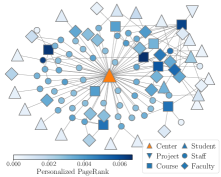
(a) Local AGG

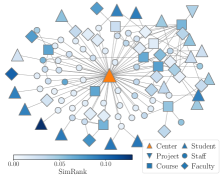
(b) SimRank AGG

(c) SimRank Diagram

Figure 1: (a) Neighborhood-based local aggregation and (b) SimRank aggregation on Texas heterophily graph. Node color represents aggregation score with respect to the center node ($\blacktriangle$ in orange). Conventional aggregation focuses on nearest nodes regardless of node label, while SimRank succeeds in assigning high values for nodes with same label ($\blacktriangle$ in blue). (c) Simrank illustration on a social network. Two professors inherit high similarity because they share similar neighbors.

Putting the ideas together, we propose SIMGA, a heterophilous GNN model that can effectively capture distant structurally similar nodes for heterophilous learning, while achieving high efficiency by its one-time global aggregation whose complexity is only near-linear to the number of graph nodes $n$. To the best of our knowledge, we make the first attempt of developing an inherent relationship between SimRank structural similarity and a converging GNN, as well as integrating it into GNN designs to achieve high efficacy. Benefiting from its expressiveness attribute, SIMGA enjoys a simple model architecture and efficient calculation. Its simple feature transformation also brings fast inference and scalability to large graphs. Experiments demonstrate that our method achieves $5\times$ speed-up over the state-of-the-art GloGNN++ [18] on the pokec dataset, currently the largest heterophily dataset with 30 million edges.

We summarize our main contributions as follows: (1) We demonstrate that SimRank can be seen as a new interpretation of GNN aggregation. Based on the theory, we propose SIMGA, utilizing SimRank as the measure to aggregate global node similarities for heterophilous graphs. (2) We demonstrate SIMGA’s effectiveness by proving the grouping effect of generated node embedding matrix and design a simple but scalable network architecture that simultaneously realizes effective representation learning and efficient computation, which incorporates near-linear approximate SimRank calculation and fast computation on million-scale large graphs. (3) We conduct extensive experiments to show the superiority of our model on a range of datasets with diverse domains, scales, and heterophilies. SIMGA achieves top-tier accuracy with $5-10\times$ faster computation than the best baseline.

2 Preliminaries

[Notations]. We denote an undirected graph $G=(V,E)$ with node set $V$ and edge set $E$. Let $n=|V|$, $m=|E|$ and $d=m/n$, respectively. For each node $v$, we use $N(v)$ to denote node $v$’s neighborhood, i.e. set of nodes directly link to $v$. The graph connectivity is represented by the adjacency matrix as $A\in\mathbb{R}^{n\times n}$, and the diagonal degree matrix is $D\in\mathbb{R}^{n\times n}$. The input node feature matrix is $F\in\mathbb{R}^{n\times f}$ and we denote $Y\in\mathbb{R}^{n\times k}$ the ground truth node label one-hot matrix, where $f$ is the feature dimension and $N_{y}$ is the number of labels in classification.

[Graph Neural Network]. Graph neural network is a type of neural networks designed for processing graph data. We summarize the key operation in GNNs into two steps: Firstly, aggregating local representations: $\hat{h}_{u}^{(l)}=\emph{AGG}(\{h_{v}^{(l)}:\forall v\in N(u)\}).$ Then, combining the aggregated information with ego node to update its embeddings: $h_{u}^{(l+1)}=\emph{UPD}(h_{u}^{(l)},\hat{h}_{u}^{(l)}),$ where $h_{u}^{(l)}$ denotes the embeddings of node $u$ generated by the $l$-th layer of network. For a model of $L$ layers in total, the final output of all nodes form the embedding matrix $H^{(L)}$, which can be fed to higher-level modules for specific tasks, such as a classifier for node label prediction. AGG($\cdot$) and UPD($\cdot$) are functions specified by concrete GNN models. For example, GCN [8], representing a series of popular graph convolution networks, uses sum function for neighbor aggregation, and updates the embedding by learnable weights together with ReLU activation.

[Graph Heterophily and Homophily]. The heterophily and homophily indicate how similar the nodes in the graph are to each other. Typically, in the context of this paper, it is mainly determined by the node labels, i.e., which category a node belongs to. The homophily of a graph can be measured by metrics like node homophily [14] and edge homophily [11]. Here we employ node homophily defined as the average proportion of the neighbors with the same category of each node:

$$\mathcal{H}_{node}=\frac{1}{|V|}\sum_{v\in V}\frac{|\{u\in N(v):y_{u}=y_{v}\}|}{|N(v)|}.$$ (1)

$\mathcal{H}_{node}$ is in range $(0,1)$ and homophilous graphs have higher $\mathcal{H}_{node}$ values closer to 1. Generally, high homophily is correlated with low heterophily, and vice versa.

[SimRank] SimRank holds the intuition that two nodes are similar if they are connected by similar neighbors, described by the following recursive formula [20]:

$$\leavevmode\resizebox{281.85585pt}{}{ $S(u,v)=\begin{cases}1&(u=v)\\ \frac{c}{|N(u)||N(v)|}\sum\limits_{u^{\prime}\in N(u),v^{\prime}\in N(v)}S(u^{\prime},v^{\prime})&(u\neq v)\end{cases}$},$$ (2)

where $c\in(0,1)$ is a decay factor emperically set to 0.6. Generally, a high SimRank score of node pair $u,v$ corresponds to high structural similarity, which is beneficial for detecting similar nodes.

3 SIMGA

In this section, we first elaborate on our intuition of incorporating SimRank as a novel GNN aggregation by presenting the new interpretation between SimRank and GNN. Then we propose our SIMGA model design and analyze its scalability and complexity.

3.1 Interpreting SimRank in GNN

In graphs with node heterophily, neighboring nodes usually belong to different categories. Their feature distributions also diversify. Such disparity prevents the model to aggregate information from neighbors that is meaningful for predictive tasks such as node classification [11]. Consequently, local uniform GNN aggregation produces suboptimal results for smoothing local dissimilarity, i.e. heterophilous representations of nodes in a few hops, failing to recognize intra-class node pairs distant [21, 22]. On the contrary, it is inferred from Eq. (2) that, SimRank is defined for any given node pairs in the graph and is calculated by recognizing whole-graph structural information. Even for long distances, SimRank succeeds in assigning higher scores to structurally similar node pairs and extracts relationships globally. We validate the ability of SimRank for aggregating global homophily in Figure 2, where frequencies of the SimRank score of node pairs in six graphs are displayed. It is clearly observed that similarity values for intra-class node pairs are significantly higher than those of inter-class ones, which is useful for the model to recognize information from homophily nodes.

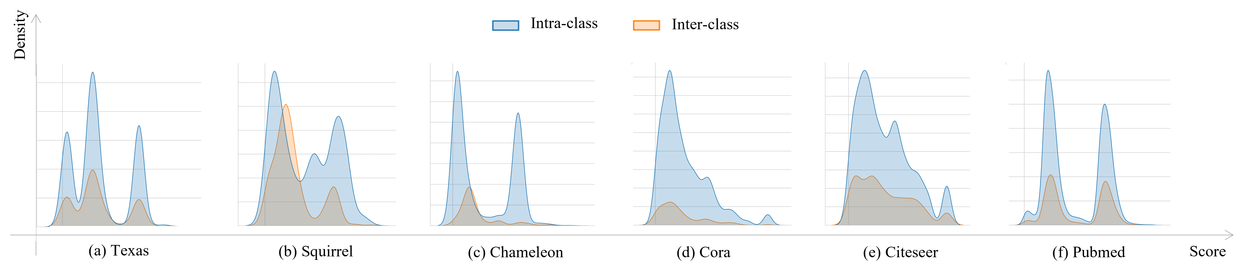
Figure 2: Distribution of SimRank scores over intra-class and inter-class node pairs. X-axis denotes the logged value for each SimRank score corresponding to one node pair and Y-axis reflects the density (frequency). Note that we filter values which are trivial, i.e. near zero.

To theoretically analyze the utilization of SimRank as GNN global aggregation, we further explore the association between SimRank and GNN. First we look into the concept of random walk:

Definition 3.1 (Pairwise Random Walk [20]).

The pairwise random walk measures the probability that two random walks starting from node $u$ and $v$ simultaneously and meet at the same node $x$ for the first time. The probability of such random-walk pairs for all tours $t^{(2l)}$ with length $2l$ can be formulated by:

$$\begin{split}P_{pair}(u,v|t^{(2l)})=\sum_{t_{u:v}^{(2l)}}P_{pair}(u,v|t_{u:v}^{(2l)})=\sum_{x\in V}p(x|u,t_{u:x}^{(l)})\cdot p(x|v,t_{v:x}^{(l)}),\end{split}$$ (3)

where $t_{u:v}^{2l}$ is one possible tour of length $2l$, $t_{v:x}^{l}:\{v,...,x\}$ is the sub-tour of length $l$ compositing the total tour, and $p(x|v,t^{(l)}_{v:x})$ denotes the probability a random walk starting from node $v$ and reaching at node $x$ under the tour $t^{(l)}_{v:x}$.

Since random walk visits the neighbors of the ego node with equal probability, $p(x|v,t^{(l)}_{v:x})$ can be trivially calculated as: $p(x|v,t^{(l)}_{v:x})=\prod_{w_{i}\in t_{v:x}}\frac{1}{|N(w_{i})|},$ where $w_{i}$ is the $i$-th node in tour $t^{(l)}_{v:x}$. Generally, a higher probability of such walks indicates a higher similarity between the source and end nodes. Pairwise random walk paves a way for node pair aggregation that can be calculated globally, compared to conventional GNN aggregation that is interpreted as random walks with limited hops, which is highly local [10, 23]. In fact, we will later show that random walk probability can be seen as GNN embeddings. In this paper, we especially consider the SGC-like architecture for representative GNN aggregation [24]. For each layer the AGG and UPD operation are accomplished by a 1-hop neighborhood propagation, and the node features are only learned before or after all layers. In other words, each intermediate layer can be written in the matrix form as $H^{(l+1)}=\mathcal{L}H^{(l)}$, where $\mathcal{L}=D^{-1}A$ denotes the graph Laplacian matrix. For other typical GNN architectures such as GCN and APPNP, similar expressions also exist [22]. We hereby present the next lemma, linking random walk and such network embeddings:

Lemma 3.2.

(See Appendix B.1 for proof). For any $l\geq 0$ and node-pair $u,v\in V$, the probability of length-$l$ random walk under all tour $t^{(l)}$ equals to the $l$-th layer embedding value $h_{u}^{(l)}[v]$ of node $u$:

$$h_{u}^{(l)}[v]=p(v|u,t_{u:v}^{(l)}).$$

Lemma 3.2 states that an $l$-layer GNN is able to simulate $l$-length random walks and its embedding contains the information of the each node’s reaching possibility. This conclusion is in line with other studies and displays the expressiveness of GNN in graph learning [10, 24, 22]. Based on the connection, we investigate a GNN mapping function $\mathcal{G}$ stacking multiple SGC layers. We are specifically interested in the case when network converges to infinity layers $L\rightarrow\infty$, denoted as $\mathcal{G}^{(\infty)}$. We derive SimRank as the novel interpretation of such GNN model in the following theorem:

Theorem 3.3.

(See Appendix B.2 for proof). On a graph $G=(V,E)$, the SimRank matrix calculated by Eq. (2) is $S$. Then, the SimRank value $S(u,v)$ of node-pair $u,v\in V$ is equivalent to the layer-wise summation of inner-product of network $\mathcal{G}^{(\infty)}$ node representations $h_{u}^{(l)},h_{v}^{(l)}$, with a decay factor $c$:

$$S(u,v)=\sum_{l=1}^{\infty}\ c^{l}\cdot\langle h_{u}^{(l)},h_{v}^{(l)}\rangle,$$ (4)

where $h_{u}^{(l)}$ is node $u$ embedding generated by $l$-th layer of $\mathcal{G}^{(\infty)}$, and $\langle\cdot\ ,\ \cdot\rangle$ denotes the inner product.

3.2 SIMGA Workflow

The implication of Theorem 3.3 is that, by calculating the SimRank matrix, it naturally retrieves the information that common GNN architectures can only represent after a number of local aggregations. As SimRank assigns high scores to node relations with topological similarities, it can be regarded as a powerful global aggregation for GNN representation, guiding the network to put higher weights on such distant but homophilous node pairs. Hence, our goal is to design effective and efficient model architecture that exploits the desirable capability of SimRank.

Considering SimRank already carries global similarity information implicitly, our model removes the need of iteratively aggregating and updating embeddings by incorporating the similarity matrix such as [17, 18]. Instead, we employ a precomputation process to acquire the SimRank matrix $S$ and only apply it once as model aggregation. Since the aggregation is as straightforward as a matrix multiplication, we establish the simple but effective transformation scheme to concatenate and learn node attributes and local adjacency. In a nutshell, the architecture of SIMGA is summarised as:

$$Z_{Sim}=\emph{SoftMax}(S\cdot f_{\theta}(F,A)),$$ (5)

where $f_{\theta}$ is a mapping function to transform features $F$ and adjacency $A$ into node embeddings. Here $S$ plays the role of final and global aggregation which gather information for all nodes according to the SimRank scores as weights. To further explain why SIMGA is effective, we mark that SIMGA in the form of Eq. (5) shares a similar idea to the representative message-passing model APPNP [10], whereas the latter follows a local propagation according to the Personalized PageRank matrix $\Pi$, while ours spotlights $S$ for global similarity measure in heterophilous settings. As a natural merit, our SIMGA satisfies various advantages of decoupled GNN models like APPNP, ranging from batch computation to scalability on large graphs.

In specific, SIMGA firstly uses two MLPs to embed node feature matrix and adjacency matrix respectively. Then, it linearly combines them with the tunable parameter $\delta\in[0,1]$, namely the feature factor, after which the concatenation is fed into a main MLP network:

$$\begin{split}H_{F}=\textit{MLP}_{F}(F),\;H_{A}=\textit{MLP}_{A}(A);\quad\quad H=\textit{MLP}_{H}\big{(}\delta\cdot H_{F}+(1-\delta)\cdot H_{A}\big{)},\end{split}$$ (6)

where $H_{F}\in\mathbb{R}^{n\times N_{y}}$ and $H_{A}\in\mathbb{R}^{n\times N_{y}}$ represents the intermediate embeddings of feature and adjacency, $H\in\mathbb{R}^{n\times N_{y}}$ is the main node embedding, and $N_{y}$ is the number of categories. Then to conduct SimRank aggregation, we apply the score matrix $S$ to the main embedding as $S\cdot H$. Referencing the common approach in Klicpera et al. [10], we adopt skip connection with tunable parameter $\alpha\in[0,1]$ to balance global aggregation and raw embeddings:

$$Z=(1-\alpha)\cdot S\cdot H+\alpha\cdot H.$$ (7)

We depict the model architecture in Appendix C and next we explain the expressiveness of SIMGA.

3.3 Grouping Effect

If two nodes $u,v$ share similar attributes and graph structures, their characterizations from other nodes are supposed to be close. This derives the formal definition of grouping effect as follow:

Definition 3.4.

[Grouping Effect [25]] Given the node set $V$, two nodes $u,v\in V$ and $u$-th row of $A^{k}$ and $F$ as $a_{u}^{k}$ and $x_{u}$ respectively, let $u$ -> $v$ denote the conditions that (1) $||f_{u}-f_{v}||_{2}\rightarrow 0$ and (2) $||a_{u}^{k}-a_{v}^{k}||_{2}\rightarrow 0$, $\forall k\in[1,K]$. A matrix $Z$ is said to have grouping effect if condition below meets:

$$u\rightarrow v\Rightarrow\forall p\in V,\;\;|Z(u,p)-Z(v,p)|\rightarrow 0.$$ (8)

Equipped with approximated matrix $S$, we demonstrate the effectiveness of SIMGA as follow:

Theorem 3.5.

(See Appendix B.3 for proof). Matrices $Z$ and $H$ both have grouping effect when $K>log_{c}{\epsilon}\approx 4$, where $\epsilon$ denotes the absolute error for approximately calculating $S$.

The grouping effect of $Z$ sufficiently demonstrates the effectiveness of SIMGA, that for two nodes regardless of their distance, if they share similar features and graph structures, their aggregated representations will be similar. Besides, for inter-class nodes, due to the low or near zero coefficients assigned by aggregation matrix $S$, their combined representations will hence be different. In a nutshell, SIMGA is capable of handling heterophily graphs due to the distinguishable aggregation.

3.4 Scalability & Complexity

Examining the respective stages of SIMGA, operations with dominant computation include the calculation on SimRank matrix $S$ and the final aggregation of $S\cdot H$. Without optimization, calculating matrix $S\in\mathcal{R}^{n\times n}$ based on Eq. (2) in a recursive way requires $\mathcal{O}(Tn^{2}d^{2})$ time and $\mathcal{O}(n^{2})$ space, where $T$ is the number of iterations and $d$ is the average degree of each node. In addition, the aggregation $S\cdot H$ also needs a computation time of $\mathcal{O}(N_{y}n^{2})$. This is inapplicable to graphs with large amount of nodes. Luckily, SimRank can be calculated really efficiently [26].

Algorithm 1 Localpush [27]

Graph $G$, decay factor $c$, error threshold $\epsilon$Approximate SimRank matrix $\hat{S}$

1$\hat{S}\leftarrow 0,\,R\leftarrow I$ max_(u,v) $R(u,v)>(1-c)\epsilon$

2$\hat{S}(u,v)\leftarrow\hat{S}(u,v)+R(u,v)$ $u^{\prime}\in N(u),v^{\prime}\in N(v)$

3$R(u^{\prime},v^{\prime})\leftarrow R(u^{\prime},v^{\prime})+c\cdot\frac{R(u,v)}{|N(u^{\prime})|\cdot|N(v^{\prime})|}$

4$R(u,v)\leftarrow 0$

5matrix $\hat{S}$

Table 1: Time complexity comparison with one
     hidden layer as an example.

Methods	Time Complexity
Geom-GCN[14]	$\mathcal{O}(|R|nmf)$
GPNN[15]	$\mathcal{O}(nmf)$
U-GCN[17]	$\mathcal{O}(n^{2}f)$
WR-GAT[19]	$\mathcal{O}(|R|n^{2}f)$
GloGNN++[18]	$\mathcal{O}(mf)$
SIMGA	$\mathcal{O}(knf)\unboldmath$

To solve above limitations, we first use the Localpush [27], one state-of-the-art all-pair SimRank computation algorithm with accuracy guarantee to speed up the calculation process. Its pseudo code is shown in Algorithm 1 and has the following approximation guarantee:

Lemma 3.6 ([27]).

Algorithm 1 returns an approximate SimRank matrix $\hat{S}$ in $\mathcal{O}(\frac{d^{2}}{c(1-c)^{2}\epsilon})$ time and holds that $\|\hat{S}-S\|_{max}<\epsilon$.

The accuracy of the approximate SimRank matrix is bounded by the parameter $\epsilon$  which is usually a constant representing absolute error threshold. Thus, the computation time of $S$, which is $\mathcal{O}(\frac{d^{2}}{c(1-c)^{2}\epsilon})$, becomes practical. Further, to reduce memory overhead of the SimRank matrix, we sparsify the matrix by utilizing top-$k$ pruning to select the $k$-largest scores for each node as utilized in [28]. This helps to reduce the space cost from at most $\mathcal{O}(n^{2})$ to $\mathcal{O}(kn)$, where $k$ is the number of values selected in top-$k$ pruning. By utilizing the pruned matrix, the aggregation by multiplying $S$ is also reduced to $\mathcal{O}(N_{y}kn)$. The other parts of SIMGA are all based on matrix multiplication. In Eq. (6), the computation complexities for $H_{F}$, $H_{A}$ and $H$ are $\mathcal{O}(N_{y}fn)$, $\mathcal{O}(dfn)$ and $\mathcal{O}(N_{y}^{2}n)$, respectively. Combining them together, we derive the time complexity of SIMGA as follows:

Proposition 3.7.

The total time complexity of SIMGA is $\mathcal{O}(\frac{d^{2}}{c(1-c)^{2}\epsilon}+c_{1}n)$, where $c_{1}=kN_{y}+N_{y}f+df+N_{y}^{2}\ll n$.

Based on Proposition 3.7, we conclude that SIMGA with such optimization achieves a near-linear time complexity to node numbers $n$, where $\mathcal{O}(\frac{d^{2}}{c(1-c)^{2}\epsilon})$ is insignificant when $d\ll\sqrt{n}$ and $\epsilon\sim 10^{-1}$. In Table 1, we compare the complexity of our SIMGA with heterophily GNNs regarding the cost of linking global connections in one hidden layer.

4 Related Work

GNNs achieve great advances and they usually root in graph manipulations and develop a variety of explicit designs surrounding aggregation and update schemes for effectively retrieving graph information [29, 30, 22]. GCN [8] mimics the operation in convolutional neural networks by summoning information from neighboring nodes in graphs and achieves larger receptive fields by stacking multiple layers. GCNII [31] chooses to stack network layers for a deeper model and further aggregation. GAT [9] exploits the attention mechanism for a more precise aggregation, while Mixhop [13] assigns weights to multi-hop neighbors. GraphSAGE [2] enhances the aggregation by sampling neighborhood and reduces computational overhead. APPNP [10] and SGC [24] decouple the network update by a separated local aggregation calculation and a simple feature transformation. Following works [32, 33, 34, 35] extend the design on scalability and generality.

Latest works notice the issue of graph heterophily and the limited capability of conventional GNNs. Zheng et al. [12] pointed out such limitation is due to that local neighbors are unable to capture informative nodes at a large distance. In addition, a uniform aggregation schema ignores the implicit difference of edges. Approaches addressing this heterophilous graph learning task can be mainly divided into two aspects. Some studies propose diverse modifications to widen the concept of local aggregation. H₂GCN [11] and WRGAT [19] establish new connections between graph nodes, while GGCN [36] and GPR-GNN [37] alternate the aggregation function to allow negative influence from neighboring nodes. Another series of models choose to rethink locality and introduce global information, including global attention [15, 16] and similarity measurement Jin et al. [17]. Especially, LINKX [38] and GloGNN++ [18] both employ feature-topology decoupling and simple MLP layers for embedding updates. We highlight the uniqueness of SIMGA to all the above works for its global aggregation incorporating the well-defined topological similarity.

5 Experiments

We comprehensively evaluate the performance of SIMGA, including classification accuracy as well as precomputation and training efficiency. We also provide a specific study on embedding homophily for aggregating similar nodes globally. More details can be found in Appendix.

5.1 Experiment Setup

Baselines We compare SIMGA with 11 baselines, including: (1) general graph learning models: MLP, GCN [8], GAT [9], Mixhop [13], and GCNII [31]; (2) graph convolution-based heterophilous models: GGCN [36], H₂GCN [11], GPR-GNN [37] and WRGAT [19]; (3) decoupling heterophilous models: LINKX [38] and GloGNN++ [18].

Parameter Settings We calculate exact SimRank score for small datasets, while adopting approximation in Section 3.4 with $\epsilon=0.1$ and $k=1024$, which is sufficient to derive excellent aggregation coefficients (see Section 5.4). The decay factor $c=0.6$ and $\alpha=0.5$ on all the datasets. The layer number of MLP_H is set to 1 and 2 for small and large datasets. We use the same dataset train/validation/test splits as in Pei et al. [14] and Liu et al. [16]. We conduct 5 and 10 repetitive experiments on the small and large datasets, respectively. Exploration on parameters including feature factor $\delta$, learning rate $r$, dropout $p$ and weight decay are elaborated in Appendix E and H.

5.2 Performance Comparison

Table 2: The classification accuracy (%) of SIMGA and baselines on all datasets. We mark models with first and second best performance in bold and underlined font in each dataset. Rank represents the average rankings among all the methods. OOM refers to the out-of-memory error. We also list dataset statistics including homophily value $\mathcal{H}_{node}$ defined in Eq. (1).

	Small Scale Datasets						Large Scale Datasets
	Texas	Citeseer	Cora	Chameleon	Pubmed	Squirrel	genius	arXiv-year	Penn94	twitch-gamers	snap-patents	pokec	Rank
Categories	5	6	7	5	3	5	2	5	2	2	5	2
Nodes	183	3,327	2,708	2,277	19,717	5,201	421,961	169,343	41,554	168,114	2,923,922	1,632,803
Edges	295	4,676	5,278	31,421	44,327	198,493	984,979	1,166,243	1,362,229	6,797,557	13,975,788	30,622,564
Features	1,703	3,703	1,433	2,325	500	2,089	12	128	5	7	269	65
$\mathcal{H}_{node}$	0.11	0.74	0.81	0.23	0.80	0.22	0.61	0.22	0.47	0.54	0.07	0.44
MLP	80.81 ± 4.75	74.02 ± 1.90	75.69 ± 2.00	46.21 ± 2.99	87.16 ± 0.37	28.77 ± 1.56	86.68 ± 0.09	36.70 ± 0.21	73.61 ± 0.40	60.92 ± 0.07	31.34 ± 0.05	62.37 ± 0.02	9.75
GAT	52.16 ± 6.63	76.55 ± 1.23	87.30 ± 1.10	60.26 ± 2.50	86.33 ± 0.48	40.72 ± 1.55	55.80 ± 0.87	46.05 ± 0.51	81.53 ± 0.55	59.89 ± 4.12	45.37 ± 0.44	71.77 ± 6.18	8.58
WRGAT	83.62 ± 5.50	76.81 ± 1.89	88.20 ± 2.26	65.24 ± 0.87	88.52 ± 0.92	48.85 ± 0.78	OOM	OOM	74.32 ± 0.53	OOM	OOM	OOM	8.33
H2GCN	84.86 ± 7.23	77.11 ± 1.57	87.87 ± 1.20	60.11 ± 2.15	89.49 ± 0.38	36.48 ± 1.86	OOM	49.09 ± 0.10	81.31 ± 0.60	OOM	OOM	OOM	8.04
GPR-GNN	78.38 ± 4.36	77.13 ± 1.67	87.95 ± 1.18	46.58 ± 1.71	87.54 ± 0.38	31.61 ± 1.24	90.05 ± 0.31	45.07 ± 0.21	81.38 ± 0.16	61.89 ± 0.29	40.19 ± 0.03	78.83 ± 0.05	7.62
GGCN	84.86 ± 4.55	77.14 ± 1.45	87.95 ± 1.05	71.14 ± 1.84	89.15 ± 0.37	55.17 ± 1.58	OOM	OOM	OOM	OOM	OOM	OOM	7.58
GCN	55.14 ± 5.16	76.50 ± 1.36	86.98 ± 1.27	64.82 ± 2.24	88.42 ± 0.50	53.43 ± 2.01	87.42 ± 0.37	46.02 ± 0.26	82.47 ± 0.27	62.18 ± 0.26	45.65 ± 0.04	75.45 ± 0.17	7.25
MixHop	77.84 ± 7.73	76.26 ± 1.33	87.61 ± 0.85	60.50 ± 2.53	85.31 ± 0.61	43.80 ± 1.48	90.58 ± 0.16	51.81 ± 0.17	83.47 ± 0.71	65.64 ± 0.27	52.16 ± 0.09	81.07 ± 0.16	6.41
GCNII	77.57 ± 3.83	77.33 ± 1.48	88.37 ± 1.25	63.86 ± 3.04	90.15 ± 0.43	38.47 ± 1.58	90.24 ± 0.09	47.21 ± 0.28	82.92 ± 0.59	63.39 ± 0.61	47.59 ± 0.69	78.94 ± 0.11	5.30
LINKX	74.60 ± 8.37	73.19 ± 0.99	84.64 ± 1.13	68.42 ± 1.38	87.86± 0.77	61.81 ± 1.80	90.77 ± 0.27	56.00 ± 1.34	84.71 ± 0.52	66.06 ± 0.19	61.95 ± 0.12	82.04 ± 0.07	5.25
GloGNN++	84.05 ± 4.90	77.22 ± 1.78	88.33 ± 1.09	71.21 ± 1.84	89.24 ± 0.39	57.88 ± 1.76	90.91 ± 0.13	54.79 ± 0.25	85.74 ± 0.42	66.34 ± 0.29	62.03 ± 0.21	83.05 ± 0.07	2.58
SIMGA	84.87 ± 4.39	77.52 ± 1.52	88.41 ± 1.33	72.00 ± 1.70	89.56 ± 0.31	62.04 ± 1.68	90.94 ± 0.52	55.16 ± 0.33	86.31 ± 0.36	66.47 ± 0.27	63.00 ± 0.16	82.33 ± 0.06	1.25

We measure our SIMGA’s performance against 11 baselines on 12 benchmark datasets of both small and large scales as Table 2, where we also rank and order the models based on respective accuracy. We stress the effectiveness of SIMGA by concluding the following observations:

• Common graph learning models generally perform worse. Among MLP, GAT, and GCN, GCN achieves the highest ranking 7.25 over all datasets. The reason may be that they fail to distinguish the homophily and heterophily nodes due to the uniform aggregation design. It is surprising that MLP only utilizing node features learns well on some datasets such as Texas, which indicates that node features are important in heterophilous graphs’ learning. Meanwhile, Mixhop and GCNII generally hold better performance than the plain models. On pokec, the accuracy for Mixhop and GCNII are 81.07 and 78.94, outperforming the former three models significantly. They benefit from strategies considering more nodes in homophily and combine node representations to boost the performance, showing the importance of modifying the neighborhood aggregation process.

• With respect to heterophilous models, those graph convolution-based approaches enjoy proper performance on small graphs by incorporating structural information, but their scalability is a bottleneck. Specifically, GGCN, H₂GCN, and WRGAT cannot be employed in most large datasets due to their high memory requirement for simultaneously processing features and conducting propagation, which hinders their application. GPR-GNN, on the contrary, shows no superiority in effectiveness. On the other hand, decoupling heterophilous models LINKX and GloGNN++ achieve the most competitive accuracy over most datasets where LINKX separately embeds node features and graph topology and GloGNN++ further performs node neighborhood aggregation from the whole set of nodes in the graph, bringing them performance improvement. Notably, the advantage of LINKX is not consistent and is usually better on large graphs than on smaller ones.

• Our method SIMGA achieves outstanding performance with the highest average accuracy on 9 out of 12 datasets and the top ranking 1.25, significantly better than the runner-up GloGNN++. We state that the superior and stable performance over various heterophilous graphs is brought by the capability of global aggregation that exploits structural information and evaluates node similarity. The simple decoupled feature transformation network architecture also effectively retrieves node features and generates embeddings. Specifically, on datasets like snap-patents, SIMGA outperforms the runner-up methods by nearly 1%., a significant improvement indicating that our method aggregates excellent neighborhood information to distinguish the homophily and heterophily. Besides, we consider SIMGA being slightly worse than the best method in three datasets due to the shallow feature transformation layers, which may have insufficient capacity for a large amount of input information and can be improved by introducing more specific designs. We leave this for future.

5.3 Efficiency Study

To evaluate the efficiency aspect of SIMGA, we investigate its learning time and convergence on 6 large-scale datasets as shown in Table 3 and Figure 3, respectively.

Table 3: The average learning time (s) of decoupling heterophily methods on 12 datasets. We separately show the precomputation and training time of SIMGA. The fastest is marked in bold.

	Texas	Citeseer	Cora	Chameleon	Pubmed	Squirrel	genius	arXiv-year	Penn94	twitch-game	snap-patents	pokec
LINKX	8.6	19.0	12.4	12.9	20.1	19.9	292.3	51.2	112.1	302.7	701.8	2472.9
GloGNN++	7.41	12.7	11.4	10.8	13.7	13.7	358.7	134.1	183.5	783.0	732.9	1564.7
SIMGA	4.3	10.2	6.6	7.5	12.1	12.7	153.6	36.5	17.2	236.5	408.2	388.5
precomp	0.0	0.1	0.2	0.1	1.6	0.3	8.6	9.3	3.9	14.0	15.9	11.4
training	4.3	10.1	6.4	7.4	10.5	12.4	145.0	27.1	13.3	222.5	392.3	377.1

Learning Time We compare the learning time of SIMGA with LINKX and GloGNN++ as they are all decoupling heterophilous methods and achieve first-tier performance. Learning time is the sum of pre-computation time and training time, since SIMGA needs to calculate the aggregation matrix before conducting network training. We use the same training set on each dataset and run 5-repeated experiments for 500 epochs. The average learning time is reported in Table 3.
It can be seen that SIMGA costs the least learning time over all the 12 datasets, especially on the large ones, thanks to its scalable pre-computation and top-$k$ global aggregation mechanism. The result aligns with our complexity analysis in Section 3.4. Besides, the one-time similarity measurement calculation in SIMGA also benefits its speed compared with the GloGNN++’s to-be-updated measurement. On datasets such as Penn94 and pokec, it outperforms GloGNN++ by around $10\times$ faster, which is a significant speed-up. Although LINKX is relatively fast due to its simple yet effective architecture, it is still slower than SIMGA, i.e. 5 times slower on the largest dataset pokec.

Convergence We then study the convergence time as another indicator of model efficiency in graph learning. We compare SIMGA against models with leading efficacy in Table 2 in Figure 3. Among the methods, MixHop and GCNII are GNNs containing multi-hop neighbors as the ego node’s neighborhood for aggregation or combine nodes with their degree information, while LINKX and GloGNN++ are decoupling heterophily methods without explicit graph convolution operation. Both SIMGA and GloGNN++ select nodes from the whole set of nodes in the graph, while SIMGA only considers nodes with significant scores and filters irrelevant ones through the top-$k$ pruning.
Figure 3 shows that SIMGA shares favorable convergence states among all graphs, i.e. achieves high accuracy in a short training time. Generally, SIMGA and LINKX are the two fastest models among all competitors. GloGNN++ can converge to the first-tier results, but its speed is usually slower than SIMGA. For example, on the largest dataset pokec with over 1.6 million nodes, SIMGA is approximately 5$\times$ faster than GloGNN++. For Penn94, the speed difference even reaches 10$\times$. Other methods such as MIXHOP is exceeded by a larger extent. These results validate that SIMGA is both highly effective and efficient, and can be capably applied to large heterophilous graphs.

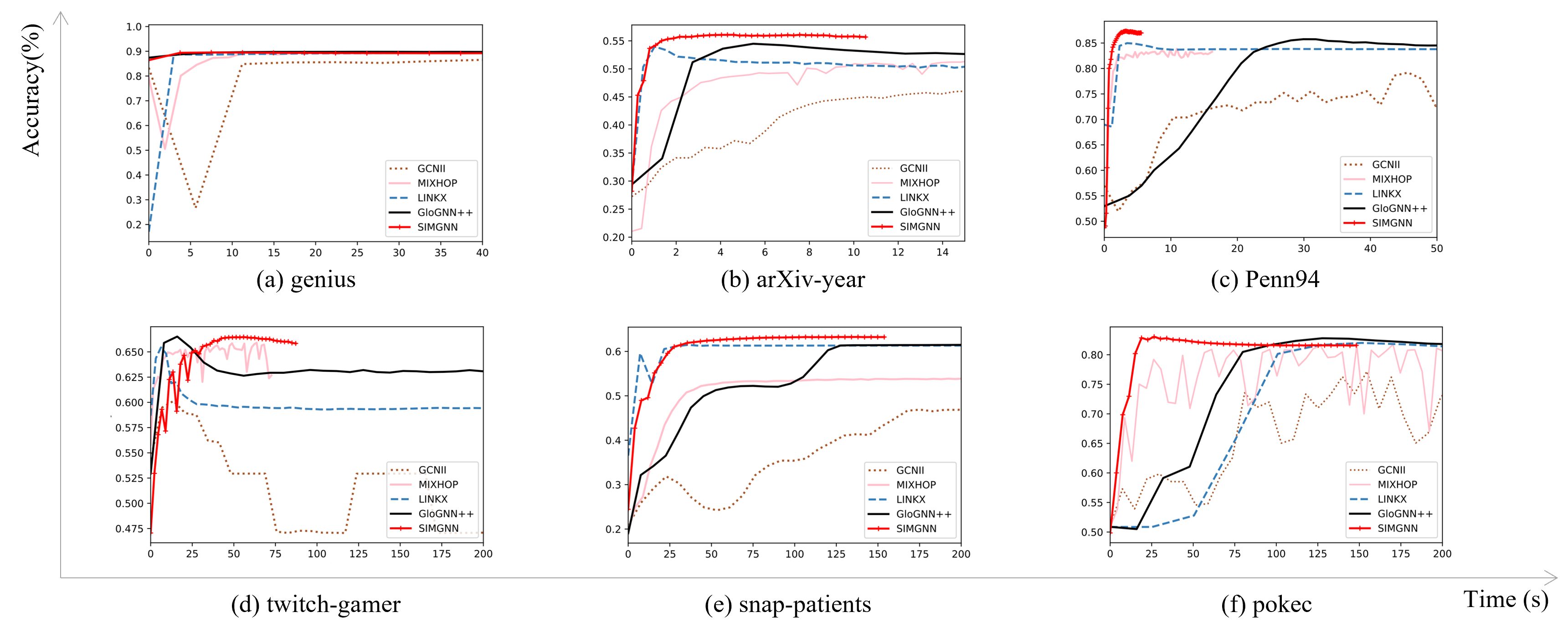
Figure 3: Convergence efficiency of SIMGA and selected baselines. X-time (s) and Y-accuracy.

5.4 Ablation Study

Parameter $\boldsymbol{\delta}$ and $\mathbf{S}$. In the initial embedding formation of SIMGA, the node attribute matrix and adjacency matrix are transformed into vectors using two MLPs. These vectors are then combined using the parameter $\delta$ in Eq.(6). To investigate the importance of these two sources of information, we consider two variants: SIMGA-NA and SIMGA-NF. SIMGA-NA removes the adjacency matrix ($\delta=0$), while SIMGA-NF removes the node attributes ($\delta=1$). After obtaining the initial embeddings $H$, SIMGA aggregates each node’s features using $S$ in Eq.(7) to capture distant intra-class nodes. We denote the variant that excludes the aggregation matrix $S$ as SIMGA-NS. The results on large-scale datasets, as shown in Figure 4(a), indicate that removing either matrix leads to a performance drop. This demonstrates the effectiveness of the aggregation process $S$ and highlights the benefits of incorporating both node attributes and the adjacency matrix in forming initial node embeddings.

(a) Parameter $\boldsymbol{\delta}$ and $\mathbf{S}$ over six large datasets. X-axis den
-otes dataset and Y-axis the accuracy.

(b) Parameter $\mathbf{k}$ and $\boldsymbol{\epsilon}$ on pokec, Citeseer and cora. Higher accuracy shows deeper color (blue).

Figure 4: Parameter effect of $\delta$, $S$, $k$ and $\epsilon$. $\delta$ denotes the balancing factor in Eq.(6), $k$ denotes number of selected nodes, $S$ the aggregation matrix and $\epsilon$ the absolute error tolerance for $S$.

Parameter $\mathbf{k}$ and $\boldsymbol{\epsilon}$. Choosing larger values for $k$ and smaller values for $\epsilon$ in the calculation of $S$ introduces increased computational complexity (Proposition 3.7). In our empirical evaluation (Figure 4(b)), we observed that setting $\epsilon=0.1$ provides satisfactory classification scores for the largest dataset, pokec. More stringent accuracy requirements by setting $\epsilon=0.01$ only yield minimal performance improvements while significantly inflating pre-computation time by approximately 100 times. Similarly, we found that larger values of $k$ lead to better results. Notably, setting $k=1024$ already achieves excellent performance, and the amount of information filtered in $S$ becomes negligible (refer to Appendix E for a more detailed discussion).

6 Conclusion

In this paper, we propose SIMGA, a simple and effective heterophilous graph neural network with near-linear time efficiency. We first derive a new interpretation of SimRank as global GNN aggregation, highlighting its capability of discovering structural similarity among nodes which are distant and have same label in the whole graph. Based on this connection, we employ a decoupling GNN architecture and utilize SimRank as aggregation without iterative calculation, where efficient approximation calculation can be applied and realize a time complexity near-linear to $n$.

Appendix A Artifact Availability

Our code is available in the anonymized URL: https://github.com/ConferencesCode/SIMGA/tree/master.

Appendix B Proof

B.1 Lemma 3.2

Proof.

We here prove Lemma 3.2 by mathematical induction. At the initial part, when $l=0$, input of the whole network is $H^{(0)}=I$ [39].

When $l=1$, based on the update scheme there is $H^{(1)}=D^{-1}A$. Note that the element for node $u$ in the diagonal degree matrix is $D_{u}=|N(u)|$. Thence, $h_{u}^{(1)}[v]$, being the entry in $H^{(1)}$ of location $(u,v)$, equals to the probability of directly walking from node $u$ to $v$ as:

$$h_{u}^{(1)}[v]=A_{u}[v]\cdot\frac{1}{|N(u)|}=p(v|u,t_{u:v}^{(1)}).$$ (9)

In the inductive case where $l>1$, assume $h_{u}^{(l-1)}[v]=p(v|u,t_{u:v}^{(l-1)})$ holds for $l-1$. Then for layer $l$ we have:

$$\begin{split}h_{u}^{(l)}[v]=&\sum_{x\in N(v)}\frac{1}{|N(x)|}\cdot h_{u}^{(l-1)}[x]\\ =&\sum_{x\in N(v)}p(v|x,t_{x:v}^{(1)})\cdot p(x|u,t_{u:x}^{(l-1)})\\ =&\quad p(v|u,t_{u:v}^{(l)}),\end{split}$$ (10)

where the first equality follows graph aggregation, and the second line is from Eq. (9). Lemma 3.2 thus holds by combining Eq. (9) and Eq. (10). ∎

B.2 Theorem 3.3

Proof.

We consider the right term of Eq. (4) by substituting Definition 3.1 and Lemma 3.2:

$$\small\begin{split}\sum_{l=1}^{\infty}c^{l}\cdot\langle h_{u}^{(l)},h_{v}^{(l)}\rangle&=\sum_{l=1}^{\infty}c^{l}\cdot\sum_{x\in V}p(x|u,t_{u:x}^{(l)})\cdot p(x|v,t_{v:x}^{(l)})\\ &=\sum_{l=1}^{\infty}c^{l}\cdot\sum_{t^{(2l)}}p(x|u,t^{(l)}_{u:x})\cdot p(x|v,t^{(l)}_{v:x})\\ &=\sum_{l=1}^{\infty}c^{l}\cdot P_{pair}(u,v|t^{(2l)})\end{split}$$

Denoted $S^{\prime}(u,v)=\sum_{l=1}^{\infty}c^{2l}\cdot P_{pair}(u,v|t^{(2l)})$, it can be easily verified that $S^{\prime}(u,v)=1$ if $u=v$, and $S^{\prime}(u,v)=0$ if there is no tour $t$ consisting of two separate random walk paths starting from $u$ and $v$ and ends in any same node $x$. Thus in general, $S^{\prime}(u,v)\in[0,1]$ holds for all node pair $(u,v)$. Then, by performing one step random walk for node $u$ and $v$, we split the sum above as follow:

$$\begin{split}S^{\prime}(u,v)=&\sum_{l^{\prime}\geq 0}\;\sum_{u^{\prime}\in N(u),v^{\prime}\in N(v)}P(u|u^{\prime},t^{(1)})\cdot P(v|v^{\prime},t^{(1)})\cdot P_{pair}^{(u^{\prime},v^{\prime}|t^{l^{\prime}})}\cdot c^{(l^{\prime}+1)}\\ =&\sum_{l^{\prime}\geq 0}\;\sum_{u^{\prime}\in N(u),v^{\prime}\in N(v)}\frac{1}{|N(u)||N(v)|}\cdot P_{pair}^{(u^{\prime},v^{\prime}|t^{l^{\prime}})}\cdot c^{(l^{\prime}+1)}\\ =&\frac{c}{|N(u)||N(v)|}\sum_{u^{\prime}\in N(u),v^{\prime}\in N(v)}\sum_{l^{\prime}\geq 0}\cdot P_{pair}^{(u^{\prime},v^{\prime}|t^{l^{\prime}})}\cdot c^{l^{\prime}},\end{split}$$ (11)

Since for $u^{\prime}\neq v^{\prime}$, $P_{pair}(u^{\prime},v^{\prime}|t^{0})=0$, we have:

$$\begin{split}S^{\prime}(u,v)&=\frac{c}{|N(u)||N(v)|}\sum_{u^{\prime}\in N(u),v^{\prime}\in N(v)}\sum_{l^{\prime}\geq 1}\cdot P_{pair}^{(u^{\prime},v^{\prime}|t^{l^{\prime}})}\cdot c^{l^{\prime}}\\ &=\frac{c}{|N(u)||N(v)|}\sum_{u^{\prime}\in N(u),v^{\prime}\in N(v)}S^{\prime}(u^{\prime},v^{\prime}).\end{split}$$ (12)

Here, Eq. (12) is exactly identical to the original SimRank equation Eq. (2) with the decay factor $c$ in SimRank. With the uniqueness of the solution to Eq. (2), we conclude that $S^{\prime}(u,v)=S(u,v)$. Thus, the proof completes. ∎

B.3 Theorem 3.5

Recall that the overall formulation for SIMGA is :

$$\begin{split}&H=\delta\cdot f_{mlp}(F)+(1-\delta)\cdot f_{mlp}(A),\\ &Z=(\alpha\cdot S+(1-\alpha)\cdot I)\cdot H.\end{split}$$ (13)

Our proof consists of three main steps by (1) Matrix $H$ holds the grouping effect; (2) By a slight diagonal adjust, matrix $\hat{S}$ holds the grouping effect and (3) Matrix Z holds the grouping effect.

Proof.

For node $u,v$ meets the condition defined by grouping effect (Definition 3.4), we have:

$$||f_{u}-f_{v}||_{2}\rightarrow 0,$$

and

$$||a_{u}^{k}-a_{v}^{k}||_{2}\rightarrow 0,\forall k\in[1,K].$$

For $\forall p\in V$,

$$\begin{split}H(u,p)-H(v,p)&=\delta\cdot\left[f_{mlp}(F)_{u,p}-f_{mlp}(F)_{v,p}\right]+(1-\delta)\cdot\left[f_{mlp}(A)_{u,p}-f_{mlp}(A)_{v,p}\right]\\ &\leq\delta\cdot\left[\sum_{k\in V}{|F_{u,k}-F_{v,k}|\cdot W_{k,p}}\right]+(1-\delta)\cdot\left[\sum_{k\in V}{|A_{u,k}-A_{v,k}|\cdot W_{k,p}}\right]\\ \end{split}$$ (14)

Thus,

$$||H(u,p)-H(v,p)||_{2}\leq\delta^{2}\cdot||W_{:,p}||_{2}\cdot||f_{u}-f_{v}||_{2}+(1-\delta)^{2}\cdot||W_{:,p}||_{2}\cdot||a_{u}^{1}-a^{1}_{v}||_{2}\rightarrow 0.$$ (15)

Hence, matrix $H$ has grouping effect.

Next we consider matrix $S$. Its T-iteration approximation matrix $S^{T}$ is computed based on the formula from [28], with $\epsilon$ absolute error bound as follow:

$$\begin{split}\forall u,v,|S_{u,v}-S^{T}_{u,v}|<\epsilon\rightarrow S^{T}=\sum_{k=0}^{T=\lceil\log_{c}\epsilon\rceil}\;c^{k}\cdot(P)^{k}D(P^{t})^{k},\quad\text{where}\;D=(1-c)\cdot I.\end{split}$$ (16)

Since $\forall k\in[1,K],P^{k}=(D^{-1}A)^{k}.$ We have the $u$-th row of $P^{k}$ as:

$$p_{u}^{k}=d_{u}^{k}\cdot a_{u}^{k},\;\text{where}\quad d_{u}=\sum_{p\in V}a_{u}^{1}[p].$$ (17)

With $||a_{u}^{k}-a_{v}^{k}||_{2}\rightarrow 0$, we have $||d_{u}^{k}-d_{v}^{k}||_{2}\rightarrow 0$, hence $||p_{u}^{k}-p_{v}^{k}||_{2}\rightarrow 0$.

Next, we show that matrix $S^{*}=S-(1-c)\cdot I$ has grouping effect:

$$\begin{split}S^{*}_{u,p}-S^{*}_{v,p}&=\sum_{k=1}^{\lceil\log_{c}\epsilon\rceil}c^{k}\cdot(1-c)\cdot\left[p_{u}^{k}\cdot(p_{p}^{k})^{t}-p_{v}^{k}\cdot(p_{p}^{k})^{t}\right]\\ &=\sum_{k=1}^{\lceil\log_{c}\epsilon\rceil}\left[p_{u}^{k}-p_{v}^{k}\right]\cdot\left[c^{k}\cdot(1-c)\cdot(p_{p}^{k})^{t}\right]\\ \xRightarrow{(K>\log_{c}\epsilon)}||S^{*}_{u,p}-S^{*}_{v,p}||_{2}&\leq\sum_{k=1}^{\lceil\log_{c}\epsilon\rceil}||p_{u}^{k}-p_{v}^{k}||_{2}\cdot||c^{k}\cdot(1-c)\cdot(p_{p}^{k})^{t}||_{2}\\ &\leq\lceil\log_{c}\epsilon\rceil\cdot||c\cdot(1-c)\cdot p_{p}^{1}||_{2}\cdot||p_{u}^{k}-p_{v}^{k}||_{2}\rightarrow 0.\end{split}$$ (18)

Thus, the matrix $S^{*}$ hold the expected grouping effect. Based on this, we transform Eq.(LABEL:eq13) into:

$$\centering\begin{split}Z=(\alpha\cdot S^{*}&+(1-\alpha\cdot c)\cdot I)\cdot H=\alpha\cdot S^{*}\cdot H+(1-\alpha\cdot c)\cdot H,\\ \Rightarrow Z_{u,p}-Z_{v,p}&=\alpha\cdot(S^{*}_{u,:}-S^{*}_{v,:})\cdot H_{:,p}+(1-\alpha\cdot c)\cdot(H_{u,p}-H_{v,p}),\\ \Rightarrow||Z_{u,p}-Z_{v,p}||_{2}&\leq 2\cdot\alpha\cdot||H_{:,p}||_{2}\cdot||S^{*}_{u,:}-S^{*}_{v,:}||_{2}+2\cdot(1-\alpha\cdot c)^{2}\cdot||H_{u,p}-H_{v,p}||_{2}\\ \end{split}\@add@centering$$ (19)

Since both matrices $S*$ and $H$ have grouping effect:

$$||S^{*}_{u,:}-S^{*}_{v,:}||_{2}\rightarrow 0,||H_{u,p}-H_{v,p}||_{2}\rightarrow 0,$$ (20)

Based on Eq.(19) we have:

$$||Z_{u,p}-Z_{v,p}||_{2}\rightarrow 0.$$ (21)

Therefore, matrices $H$, $Z$ and $S^{*}$ all have desired grouping effect, the proof completes. ∎

Appendix C Architecture of SIMGA

The architecture of SIMGA can be summarized as depicted in Figure 5. The SIMGA framework follows a step-by-step process to transform the input data and perform classification. Initially, SIMGA takes the node features and adjacency matrix as separate inputs. These inputs are individually processed through a linear combination of two Multilayer Perceptrons (MLPs) denoted as $MLP_{F}$ and $MLP_{A}$. It is important to note that in this study, both $MLP_{F}$ and $MLP_{A}$ are set to have a single layer. Following the embedding of node features and the adjacency matrix, the embeddings are then aggregated using the SimRank measurement. SimRank captures the similarity between nodes in a graph based on their structural relationships, and this aggregation step helps to incorporate global structural information into the embeddings. Finally, the aggregated embeddings, along with a skip connection, are passed into a SoftMax classifier.

Figure 5: Architecture of SIMGA.

By employing this architecture, SIMGA effectively combines the information from node features and graph structure, leveraging SimRank-based aggregation to enhance the learned embeddings. The subsequent SoftMax classifier utilizes these enriched embeddings to perform classification tasks. Figure 5 visually presents an overview of this architecture within the SIMGA framework.

Appendix D Ablation Study

In this section, we conduct an abalation study on the 6 large-scale datasets to study the effect of $\delta$, the hyper-parameter balancing the feature and adjacency matrix shown on Eq.(6). We denote SIMGA-NA as $\delta=0$, where the initial node embeddings are all from the feature matrix $H_{F}$ and SIMGA-NF as $\delta=1$, where the initial node embeddings are all from the adjacency matrix $H_{A}$. The results are displayed on Figure 6.

Figure 6: Abalation study.

Based on the figure, we can see that SIMGA shows significant performance dominance over SIMGA-NA over all the datasets. Meanwhile, though SIMGA-NF is comparable with SIMGA on several datasets, SIMGA outweighs SIMGA-NF greatly on the others. This shows the importance of SIMGA to incorporate both feature and adjancy matrix to generater the initial node embeddings, since SIMGA’s aggregation mechanism considers both structure and feature similarities.

Appendix E Effect of Model Parameters

As mentioned in Section 3.4, the error bound $\epsilon$ for approximate Simrank matrix and the number of top-$k$ prunings are set to $0.1$ and $1024$, which is sufficient to achieve great performance. Here, we study the influence of different error bounds and top-$k$ purning numbers. We choose different value combinations $\epsilon$ in $[0.1,0.05,0.01]$ and $k$ in $[1,8,16,32,64,128,256,512,1024]$ and show the final accuracy performance on dataset pokec on Figure 7.

Figure 7: Parameter study.

Based on the analysis of the Figure, several observations can be made. Firstly, it is apparent that the accuracy generally improves as the number of top-$k$ accumulates. However, the improvement becomes insignificant when $k$ reaches a relatively large value, such as 128. This suggests that there is a diminishing return in accuracy gains beyond a certain threshold. Moreover, SIMGA’s performance appears to be relatively insensitive to the tightness of the error bound. Even when the error bound $\epsilon$ is tightened from 0.1 to 0.01, there is no substantial improvement in performance. The increase in accuracy is only 0.03, which is negligible. However, it is important to note that the costs associated with pre-calculating the SimRank matrix $S$ significantly escalate when aiming for a tighter error bound. Therefore, to strike a balance between efficiency and performance, a general setting with $\epsilon=0.1$ and $k=1024$ is chosen.

Figure 8: Accumulated SimRank scores.

Furthermore, Figure 8 illustrates the summation of SimRank scores for different top-$k$ numbers. The black horizontal line represents the total SimRank score without top-$k$ pruning. It can be observed that with $k=1024$, the significant coefficients are sufficiently covered, making larger $k$ scales unnecessary. These findings collectively support the decision to opt for the specific settings of $\epsilon=0.1$ and $k=1024$ to ensure both efficiency and satisfactory performance. The analysis also emphasizes the importance of striking a balance between accuracy gains, computational costs, and the practicality of larger $k$ values.

Appendix F t-SNE Visualization

To intuitively demonstrate the effectiveness of our proposed model, we employ t-SNE (t-Distributed Stochastic Neighbor Embedding) [40] to visualize the output embeddings. Figure 9 showcases the t-SNE visualizations of the embeddings generated by our model across six small datasets. The visual representations reveal a coherent and compact structure, characterized by a tight clustering within individual classes and well-defined boundaries between different classes. These observations strongly support the validation of our novel concept of SimRank-based aggregation in SIMGA (SimRank-based Graph Aggregation). The compelling results obtained through t-SNE provide tangible evidence of the improved performance and discriminative power of our proposed model.

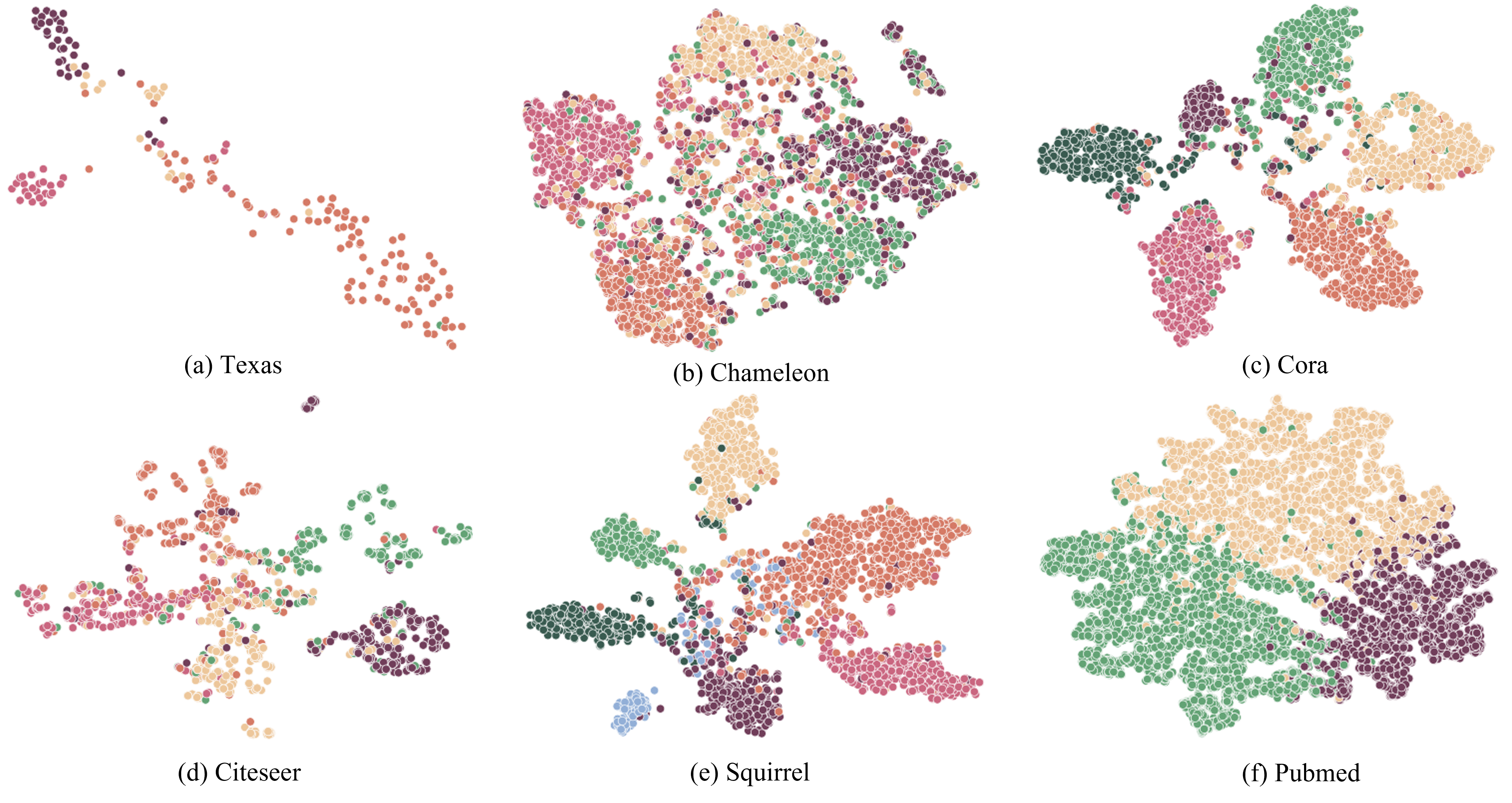
Figure 9: T-sne visualization of SIMGA over six small datasets. Different colors correspond to different ground truth classes.

Appendix G Grouping Effect

To effectively demonstrate the prowess of our proposed model, we present the output embedding $Z$ as defined in Eq. (7), showcasing its application on six small-scale graphs in Figure 10. In accordance with Theorem 3.4, the $Z$ matrix exhibits the desired grouping effect, aligning perfectly with the visual representation. Upon close examination, we can distinctly observe that nodes belonging to the same category labels exhibit strikingly similar embedding vector patterns generated by SIMGA. Conversely, nodes from different labels manifest clear distinctions from one another.

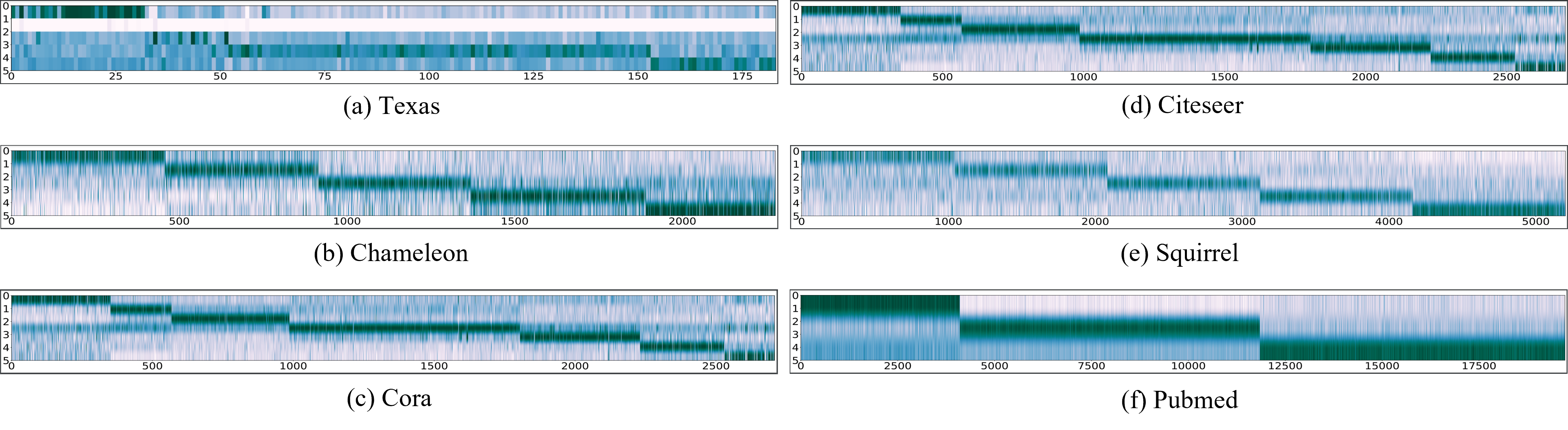
Figure 10: Homophily in node embeddings $Z$. X-axis corresponds to node index reordered by category labels, color along Y-axis represents values in the node embedding vector.

For instance, in Figure 10, the Pubmed dataset, encompassing three distinct node types, displays separate rectangular patterns for each category. This phenomenon vividly illustrates a high degree of inter-group homophily and intra-group heterophily. Notably, the number of observed patterns aligns precisely with the category count within each dataset, thereby further reinforcing SIMGA’s capacity to capture global node homophily while effectively distinguishing heterophily. These findings serve as compelling evidence of SIMGA’s effectiveness in capturing nuanced structural characteristics and validating its ability to discern between different node categories.

Appendix H Dataset-specific Settings

We conduct experiments on 12 real-world datasets, including 6 small-scale and 6 large-scale datasets spanning various domains, features, and graph homophiles. Among them, Texas, Chameleon, and Squirrel [41] are three webpage datasets collected from Wikipedia or Cornell University with low homophily ratios. Cora, Citeseer, Pubmed, Arxiv-year and Snap-patents [42, 43, 44, 45, 46] are citation graphs where the first three have high and the last two have low homophily ratios. Penn94, pokec, Genius, and twitch-gamers [38] are all social networks extracted from online websites such as Facebook, having moderate homophily ratios. The statistics containing number of nodes, edges, categories, and features, as well as homophily ratios are summarized in Table 2.

Table 4: Grid search range on small-scale datasets

	Range
Parameter	Small Datasets	Large Datasets
feature factor $\delta$	{0, 0.1, 0.2, …, 1}	{0, 0.5, 1}
dropout $p$	{0, 0.1, 0.2, …, 0.9}	{0, 0.1, 0.2, …, 0.9}
learning rate $r$	[$1e-6,1e-2$]	{1e-2, 1e-4, 1e-5}
weight decay	[0, $1e-2$]	{0, 1e-3, 1e-5}
hidden layer dim	{32, 64, 128, 256}	{32, 64, 128, 256, 512}
early stopping	{40, 100, 150, 200, 300}	{100, 300}

We apply grid searches to tune the hyper-parameters. In each dataset, we conduct tuning based on the validation results in each repeated experiments, for example every split among the 10 splits in total for small-scale datasets. We display the range of these hyper-parameter in the following Table 4 and LABEL:hyper_large. Note that the learning rate and weight decay are uniformly sampled from range $[1e-6,1e-2]$ and $[0,1e-2]$, respectively, in the small-scale datasets. All the experiments are conduct on a machine with a single Tesla V100 GPU and 40GB memory.

References

- Welling and Kipf [2016] Max Welling and Thomas N Kipf. Semi-supervised classification with graph convolutional networks. In J. International Conference on Learning Representations (ICLR 2017), 2016.
- Hamilton et al. [2017] Will Hamilton, Zhitao Ying, and Jure Leskovec. Inductive representation learning on large graphs. Advances in neural information processing systems, 30, 2017.
- Yow and Luo [2022] Kai Siong Yow and Siqiang Luo. Learning-based approaches for graph problems: a survey. arXiv preprint arXiv:2204.01057, 2022.
- Zhu et al. [2022] Zulun Zhu, Jiaying Peng, Jintang Li, Liang Chen, Qi Yu, and Siqiang Luo. Spiking graph convolutional networks. arXiv preprint arXiv:2205.02767, 2022.
- Fan et al. [2020] Mengzhen Fan, Dawei Cheng, Fangzhou Yang, Siqiang Luo, Yifeng Luo, Weining Qian, and Aoying Zhou. Fusing global domain information and local semantic information to classify financial documents. In Proceedings of the 29th ACM International Conference on Information & Knowledge Management, pages 2413–2420, 2020.
- Wang et al. [2021a] Hanzhi Wang, Mingguo He, Zhewei Wei, Sibo Wang, Ye Yuan, Xiaoyong Du, and Ji-Rong Wen. Approximate graph propagation. In Proceedings of the 27th ACM SIGKDD Conference on Knowledge Discovery & Data Mining, pages 1686–1696, 2021a.
- Chen et al. [2020a] Ming Chen, Zhewei Wei, Bolin Ding, Yaliang Li, Ye Yuan, Xiaoyong Du, and Ji-Rong Wen. Scalable graph neural networks via bidirectional propagation. Advances in neural information processing systems, 33:14556–14566, 2020a.
- Kipf and Welling [2016] Thomas N Kipf and Max Welling. Semi-supervised classification with graph convolutional networks. arXiv preprint arXiv:1609.02907, 2016.
- Veličković et al. [2017] Petar Veličković, Guillem Cucurull, Arantxa Casanova, Adriana Romero, Pietro Lio, and Yoshua Bengio. Graph attention networks. arXiv preprint arXiv:1710.10903, 2017.
- Klicpera et al. [2018] Johannes Klicpera, Aleksandar Bojchevski, and Stephan Günnemann. Predict then propagate: Graph neural networks meet personalized pagerank. International Conference on Learning Representations, 2018.
- Zhu et al. [2020] Jiong Zhu, Yujun Yan, Lingxiao Zhao, Mark Heimann, Leman Akoglu, and Danai Koutra. Beyond homophily in graph neural networks: Current limitations and effective designs. Advances in Neural Information Processing Systems, 33:7793–7804, 2020.
- Zheng et al. [2022] Xin Zheng, Yixin Liu, Shirui Pan, Miao Zhang, Di Jin, and Philip S. Yu. Graph neural networks for graphs with heterophily: A survey. 2022.
- Abu-El-Haija et al. [2019] Sami Abu-El-Haija, Bryan Perozzi, Amol Kapoor, Nazanin Alipourfard, Kristina Lerman, Hrayr Harutyunyan, Greg Ver Steeg, and Aram Galstyan. Mixhop: Higher-order graph convolutional architectures via sparsified neighborhood mixing. In international conference on machine learning, pages 21–29. PMLR, 2019.
- Pei et al. [2020] Hongbin Pei, Bingzhe Wei, Kevin Chen-Chuan Chang, Yu Lei, and Bo Yang. Geom-gcn: Geometric graph convolutional networks. International Conference on Learning Representations, 2020.
- Yang et al. [2022a] Tianmeng Yang, Yujing Wang, Zhihan Yue, Yaming Yang, Yunhai Tong, and Jing Bai. Graph pointer neural networks. Proceedings of the … AAAI Conference on Artificial Intelligence, 2022a.
- Liu et al. [2021] Meng Liu, Zhengyang Wang, and Shuiwang Ji. Non-local graph neural networks. IEEE Transactions on Pattern Analysis and Machine Intelligence, 2021.
- Jin et al. [2021] Di Jin, Zhizhi Yu, Cuiying Huo, Rui Wang, Xiao Wang, Dongxiao He, and Jiawei Han. Universal graph convolutional networks. Advances in Neural Information Processing Systems, 34:10654–10664, 2021.
- Li et al. [2022] Xiang Li, Renyu Zhu, Yao Cheng, Caihua Shan, Siqiang Luo, Dongsheng Li, and Weining Qian. Finding global homophily in graph neural networks when meeting heterophily. International Conference on Machine Learning, 2022.
- Suresh et al. [2021] Susheel Suresh, Vinith Budde, Jennifer Neville, Pan Li, and Jianzhu Ma. Breaking the limit of graph neural networks by improving the assortativity of graphs with local mixing patterns. Proceedings of the 27th ACM SIGKDD Conference on Knowledge Discovery & Data Mining, 2021.
- Jeh and Widom [2002] Glen Jeh and Jennifer Widom. Simrank: a measure of structural-context similarity. In Proceedings of the eighth ACM SIGKDD international conference on Knowledge discovery and data mining, pages 538–543, 2002.
- Yan et al. [2021a] Yujun Yan, Milad Hashemi, Kevin Swersky, Yaoqing Yang, and Danai Koutra. Two sides of the same coin: Heterophily and oversmoothing in graph convolutional neural networks. arXiv preprint arXiv:2102.06462, 2021a.
- Yang et al. [2022b] Liang Yang, Wenmiao Zhou, Weihang Peng, Bingxin Niu, Junhua Gu, Chuan Wang, Xiaochun Cao, and Dongxiao He. Graph Neural Networks Beyond Compromise Between Attribute and Topology. In Proceedings of the ACM Web Conference 2022, pages 1127–1135, Virtual Event, Lyon France, April 2022b. ACM.
- Xu et al. [2018] Keyulu Xu, Chengtao Li, Yonglong Tian, Tomohiro Sonobe, Ken-ichi Kawarabayashi, and Stefanie Jegelka. Representation learning on graphs with jumping knowledge networks. In Jennifer Dy and Andreas Krause, editors, Proceedings of the 35th International Conference on Machine Learning, volume 80 of Proceedings of Machine Learning Research, pages 5453–5462. PMLR, 10–15 Jul 2018.
- Wu et al. [2019] Felix Wu, Amauri Souza, Tianyi Zhang, Christopher Fifty, Tao Yu, and Kilian Weinberger. Simplifying graph convolutional networks. In Kamalika Chaudhuri and Ruslan Salakhutdinov, editors, Proceedings of the 36th International Conference on Machine Learning, volume 97, pages 6861–6871, 6 2019.
- Li et al. [2020] Xiang Li, Ben Kao, Caihua Shan, Dawei Yin, and Martin Ester. Cast: a correlation-based adaptive spectral clustering algorithm on multi-scale data. In Proceedings of the 26th ACM SIGKDD International Conference on Knowledge Discovery & Data Mining, pages 439–449, 2020.
- Luo and Zhu [2023] Siqiang Luo and Zulun Zhu. Massively parallel single-source simranks in rounds. arXiv preprint arXiv:2304.04015, 2023.
- Wang et al. [2018] Yue Wang, Xiang Lian, and Lei Chen. Efficient simrank tracking in dynamic graphs. In 2018 IEEE 34th international conference on data engineering (ICDE), pages 545–556. IEEE, 2018.
- Tao and Li [2014] Wenbo Tao and Guoliang Li. Efficient top-k simrank-based similarity join. In Proceedings of the 2014 ACM SIGMOD International Conference on Management of Data, pages 1603–1604, 2014.
- Maron et al. [2019] Haggai Maron, Heli Ben-Hamu, Nadav Shamir, and Yaron Lipman. Invariant and equivariant graph networks. In International Conference on Learning Representations, 2019.
- Zhu et al. [2021] Meiqi Zhu, Xiao Wang, Chuan Shi, Houye Ji, and Peng Cui. Interpreting and Unifying Graph Neural Networks with An Optimization Framework. In Proceedings of the Web Conference 2021, pages 1215–1226, Ljubljana Slovenia, April 2021. ACM.
- Chen et al. [2020b] Ming Chen, Zhewei Wei, Zengfeng Huang, Bolin Ding, and Yaliang Li. Simple and deep graph convolutional networks. In International Conference on Machine Learning, pages 1725–1735. PMLR, 2020b.
- Gasteiger et al. [2019] Johannes Gasteiger, Stefan Weißenberger, and Stephan Günnemann. Diffusion Improves Graph Learning. In 32nd Advances in Neural Information Processing Systems, 2019.
- Bojchevski et al. [2020] Aleksandar Bojchevski, Johannes Klicpera, Bryan Perozzi, Amol Kapoor, Martin Blais, Benedek Rózemberczki, Michal Lukasik, and Stephan Günnemann. Scaling graph neural networks with approximate pagerank. Proceedings of the ACM SIGKDD International Conference on Knowledge Discovery and Data Mining, pages 2464–2473, 2020.
- Wang et al. [2021b] Hanzhi Wang, Mingguo He, Zhewei Wei, Sibo Wang, Ye Yuan, Xiaoyong Du, and Ji Rong Wen. Approximate Graph Propagation. In Proceedings of the ACM SIGKDD International Conference on Knowledge Discovery and Data Mining, volume 1, pages 1686–1696. Association for Computing Machinery, 2021b.
- Liao et al. [2022] Ningyi Liao, Dingheng Mo, Siqiang Luo, Xiang Li, and Pengcheng Yin. Scara: Scalable graph neural networks with feature-oriented optimization. Proceedings of the VLDB Endowment, 15(11):3240–3248, 2022.
- Yan et al. [2021b] Yujun Yan, Milad Hashemi, Kevin Swersky, Yaoqing Yang, and Danai Koutra. Two sides of the same coin: Heterophily and oversmoothing in graph convolutional neural networks. IEEE International Conference on Data Mining (ICDM 2022), 2021b.
- Chien et al. [2021] Eli Chien, Jianhao Peng, Pan Li, and Olgica Milenkovic. Adaptive universal generalized pagerank graph neural network. In International Conference on Learning Representations, 2021. URL https://openreview.net/forum?id=n6jl7fLxrP.
- Lim et al. [2021] Derek Lim, Felix Hohne, Xiuyu Li, Sijia Linda Huang, Vaishnavi Gupta, Omkar Bhalerao, and Ser Nam Lim. Large scale learning on non-homophilous graphs: New benchmarks and strong simple methods. Advances in Neural Information Processing Systems, 34:20887–20902, 2021.
- Luo et al. [2022] Linhao Luo, Yixiang Fang, Moli Lu, Xin Cao, Xiaofeng Zhang, and Wenjie Zhang. Gsim: A graph neural network based relevance measure for heterogeneous graphs. arXiv preprint arXiv:2208.06144, 2022.
- Van der Maaten and Hinton [2008] Laurens Van der Maaten and Geoffrey Hinton. Visualizing data using t-sne. Journal of machine learning research, 9(11), 2008.
- Rozemberczki et al. [2021] Benedek Rozemberczki, Carl Allen, and Rik Sarkar. Multi-scale attributed node embedding. Journal of Complex Networks, 9(2):cnab014, 2021.
- Bojchevski and Günnemann [2018] Aleksandar Bojchevski and Stephan Günnemann. Deep gaussian embedding of graphs: Unsupervised inductive learning via ranking. In International Conference on Learning Representations, 2018. URL https://openreview.net/forum?id=r1ZdKJ-0W.
- Sen et al. [2008] Prithviraj Sen, Galileo Namata, Mustafa Bilgic, Lise Getoor, Brian Galligher, and Tina Eliassi-Rad. Collective classification in network data. AI magazine, 29(3):93–93, 2008.
- Namata et al. [2012] Galileo Namata, Ben London, Lise Getoor, Bert Huang, and U Edu. Query-driven active surveying for collective classification. In 10th International Workshop on Mining and Learning with Graphs, volume 8, page 1, 2012.
- Clement et al. [2019] Colin B. Clement, Matthew Bierbaum, Kevin P. O’Keeffe, and Alexander A. Alemi. On the use of arxiv as a dataset, 2019.
- Jure Leskovec and Andrej Krevl [2014] Jure Leskovec and Andrej Krevl. Snap datasets: Stanford large network dataset collection. http://snap.stanford.edu/data, 2014.