Jump-starting relativistic flows, and the M87 jet

Abstract

We point out the dominant importance of plasma injection effects for relativistic winds from pulsars and black holes. We demonstrate that outside the light cylinder the magnetically dominated outflows while sliding along the helical magnetic field  move in fact nearly radially with very large Lorentz factors $\gamma_{0}\gg 1$, imprinted into the flow during pair production within the gaps. Only at larger distances, $r\geq\gamma_{0}(c/\Omega)$, the MHD acceleration $\Gamma\propto r$ takes over. As a result, Blandford-Znajek (BZ) driven outflows would produce spine-brightened images. The best-resolved case of the jet in M87 shows both bright edge-brightened features, as well as weaker spine-brightened feature. Only the spine-brightened component can be BZ-driven/originate from the BH’s magnetosphere.

1 Introduction

Acceleration of relativistic winds and jets is a classical problem in high energy astrophysics (e.g. Michel, 1969; Goldreich & Julian, 1970; Blandford & Znajek, 1977; Blandford & Königl, 1979; Camenzind, 1986; Krolik, 1999; McKinney, 2006; Barkov & Komissarov, 2008; Blandford et al., 2019). A standard approach involves solution of the MHD equation (analytical or numerical) starting with a slowly moving plasma. Plasma is then accelerated by the corresponding pressure gradient, and collimated by magnetic hoop stresses (Blandford & Payne, 1982).

Observations of the inner part of the jet in M87, down to just 7 Schwarzschild radii, shows complicated structure. First, one observes limb-brightened collimated jet - the jet accelerating smoothly, with a parabolic profile Nakamura & Asada (2013); Kim et al. (2018); Blandford et al. (2019), Fig. 1.

In addition to limb-brightened structures, Lu et al. (2023) recently detected a new feature - spine-brightened jet.

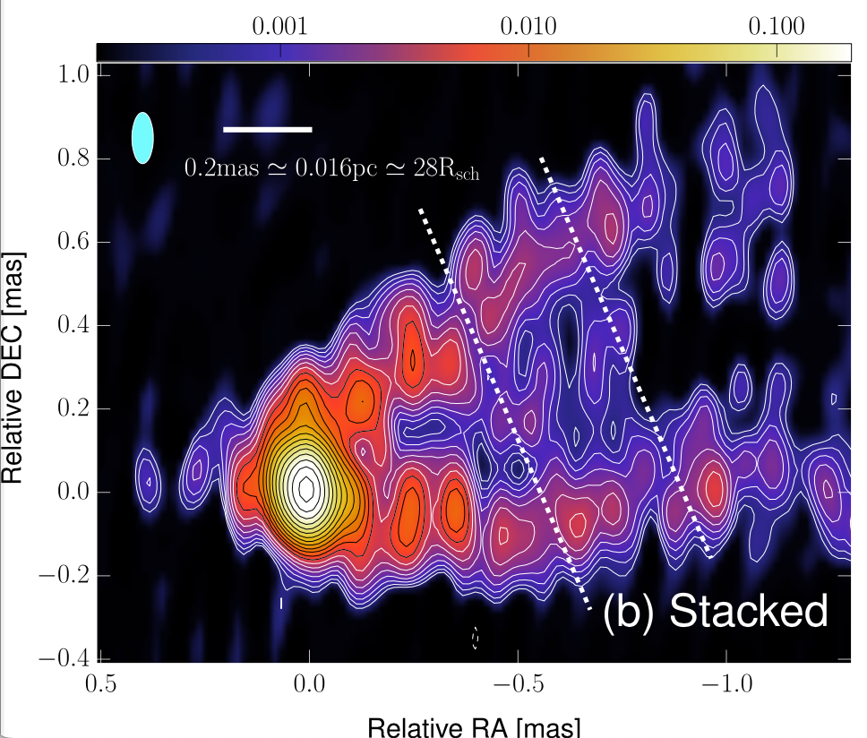
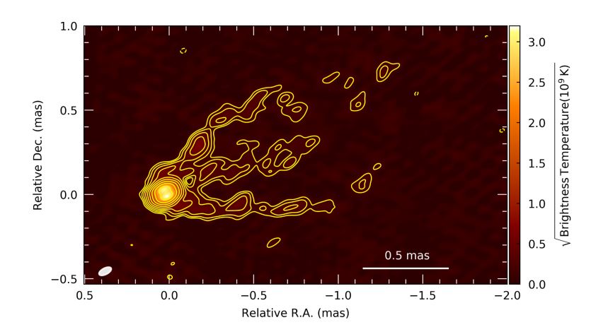
Figure 1: Top: Central part of jet in M87 at 86 GHz showing limb-brightened jet (Kim et al., 2018). Bottom: spine-brightened structure (Lu et al., 2023)

.

In this work we aim to model the emission pattern expected in the Blandford & Znajek (1977) model of jet acceleration and compare with the observation. The key new ingredient in our work is taking into account large initial (injection) velocities parallel to the local magnetic field.

MHD models of acceleration (Beskin, 2009; Komissarov et al., 2009; Nokhrina & Beskin, 2017) take full account of plasma velocity: both along and across magnetic field. The corresponding analytical treatment, based on the relativistic Grad-Shafranov equation (Grad, 1967; Shafranov, 1966; Scharlemann & Wagoner, 1973; Beskin, 2009) is completed, as it requires finding the initially unknown current distribution together with the solution for the magnetic field.

In the limit of highly magnetized plasma - the force-free limit - the parallel velocity is not defined in principle. But that does not mean it can be neglected. Plasma may be/is streaming with large Lorentz factors along magnetic fields. It seems this particular aspect was/is not considered previously. But it is highly important as we argue here.

Models of gaps in black hole magnetospheres (Hirotani & Okamoto, 1998; Blandford & Znajek, 1977; Levinson, 2000; Levinson & Rieger, 2011; Ptitsyna & Neronov, 2016) generally predict that magnetospheric gaps, with thickness much smaller than the size of the magnetosphere (the light cylinder) accelerate particles with Lorentz factors $\sim 10^{3}-10^{4}$; accelerated particles first IC scatter soft disk photons, this is followed by two-photon pair production, and the electromagnetic cascade. Resulting Lorentz factors are of similar values, $\sim 10^{3}-10^{4}$. Lorentz factors up to $\sim 10^{6}$ are also possible (Ptitsyna & Neronov, 2016).

In MHD simulations, first, high magnetization is hard to achieve and, second, plasma is typically injected at rest (e.g. Tomimatsu, 1994). In the corresponding PIC simulations particles are typically injected at rest (e.g. Chen & Beloborodov, 2014; Philippov et al., 2015; Crinquand et al., 2020; Hakobyan et al., 2022).

Perhaps the closest approach to the current one is Beskin & Kuznetsova (2000), where the importance of injection for the structure of the magnetosphere and the corresponding energy relations were discussed, quote ”it is the pair creation region that plays the role of the energy source” (Beskin et al., 1992, is also relevant).

2 The approach and the conclusion

We start with a force-free solution and add particle dynamics along the field kinematically, in the bead-on-wire approximation, neglecting its back reaction on the structure of the magnetic field. The bead-on-wire approach has a clear advantage: for a given structure of the magnetic field the particle dynamics is easily calculated in algebraic form (see also Section 7.2.6 of Gralla & Jacobson, 2014). No integration of the equations of motion is needed and no special conditions (e.g. at Alfvén or fast surfaces) appear. The drawback is that it does not provide the full picture of what the magnetic field structure is: the structured the magnetosphere  should be prescribed. Thus, our approach can be seen as the next term in expansion in magnetization parameter $1/\sigma\ll 1$: force-free solution in the limit $1/\sigma\to 0$ provide the structure of the magnetic field, the next term takes in the account particle dynamics in the prescribed magnetic field.

As a start, we assume that flow lines and magnetic flux surfaces are conical. (More complicated collimated flux surfaces behave similarly, see §6.1). In flat metrics, there is then analytical solution for the monopolar magnetic field due to Michel (1973) (it can be generalized to Schwarzschild case). We use it as a starting point:

$$B_{r}=\frac{r_{0}^{2}}{r^{2}}B_{0}\mbox{}$$

$$B_{\phi}=-\frac{r_{0}^{2}\sin\theta\Omega}{r}B_{0}=E_{\theta}\mbox{}$$

$$\vec{\beta}_{EM}=\left\{\frac{r^{2}\sin^{2}\theta\Omega^{2}}{1+r^{2}\sin^{2}\theta\Omega^{2}},0,\frac{r\Omega\sin(\theta)}{1+r^{2}\sin^{2}\theta\Omega^{2}}\right\}\mbox{}$$

$$\Gamma_{EM}=\sqrt{1+r^{2}\Omega^{2}\sin^{2}(\theta)}$$ (1)

This analytical force-free solution of the pulsar equation (Scharlemann & Wagoner, 1973; Beskin, 2009) passes smoothly through the light cylinder  (Alfvén surface) $R_{LC}=c/(\sin\theta\Omega)$. Numerical models of the inner wind indicate that the structure of the electromagnetic fields quickly approaches Michel’s solution Prokofev et al. (2018). Komissarov (2004) showed that monopolar geometry of magnetic field lines is also a good approximation in case of a black hole in external magnetic field.

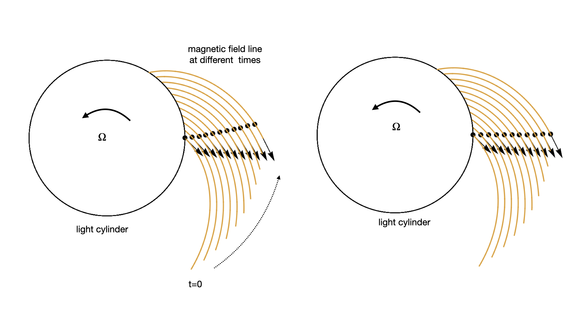
Figure 2: Particles’ trajectories calculated in Michel’s field outside the light cylinder for Lorentz factors  $\gamma_{0}=2,\,10$, Eq, (A7). The circle is the light cylinder, orange curves indicate the same magnetic field line at consecutive movements, arrows are directions of particle velocity at each point, and black dots are the location of the particle. These calculations illustrate that for $\gamma_{0}\gg 1$ the trajectory is nearly radial.

As long as the force-free condition is satisfied (negligible inertial effects) arbitrary initial motion of (charge neutral) plasma can be added along the field. Conditions at the light cylinder remain unchanged. The total velocity is then the (relativistic) sum of the electromagnetic velocity (1) and the motion along the rotating magnetic field.

It turns out that a particle launched with large Lorentz factor along the rotating magnetic spiral (in a bead-on-wire approximation) moves nearly radially, Fig. 2. This has been a known effect from numerical analysis (Contopoulos et al., 2020), and was recently analytically discussed by Lyutikov (2022). The key point is that the azimuthal motion along the spiral is nearly compensated by the motion of the spiral itself. In this paper we generalize the results of Lyutikov (2022) for particle dynamics in rotating winds to the curved space of Schwarzschild and Kerr black holes.

The observed emission pattern from relativistically moving particles is dominated by the Doppler factor $\delta$. For axisymmetric jet the largest Doppler factor is along the flow lines that project to the spine of the image, Fig. 3.

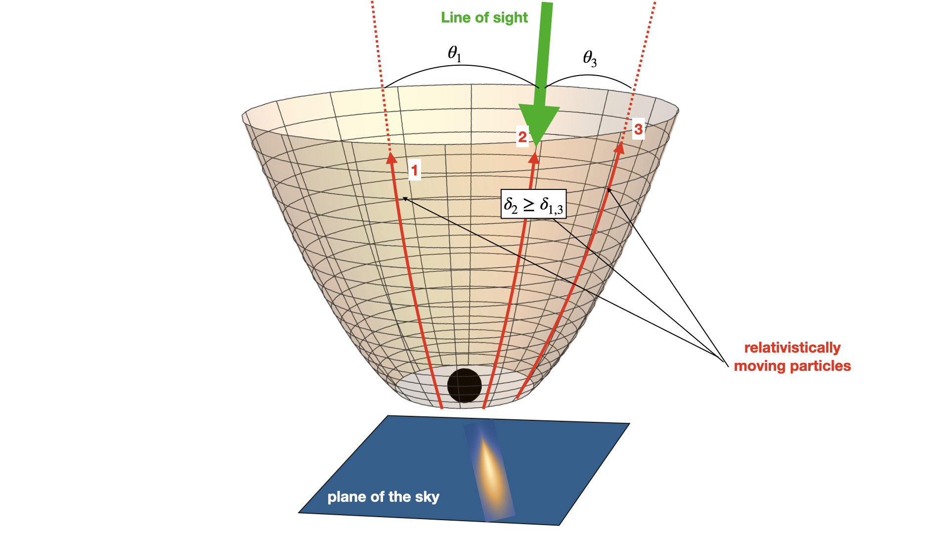
Figure 3: Graphic explanation why BZ-produced jets are expected to be spine-brightened. Shown are flux surfaces and three different particles’ trajectories. Emission produced by particle 2 has the smallest angle with respect to the line of sight, largest Doppler factor, and would result in brightest emission pattern.

Thus, relativistic flows emanating from within the magnetosphere, driven by the BZ process, are expected to produce spine-brightened image. This is consistent with observations of a weak central spine in M87 jet, Fig. 1 bottom panel. On the other hand, the edge-brightened emission observed by Kim et al. (2018) is inconsistent with the BZ process. The edge-brightened part is not centered on the black hole. This implies that a flow is only mildly relativistic. For example, estimates of the viewing angle $15^{\circ}-30^{\circ}$ degrees (Bicknell & Begelman, 1996) imply bulk Lorentz factors $\sim 3-2$ (otherwise the emission would have been beamed away).

We then conclude that the limb-brightened and spine-brightened parts of the M87 jet have different origin: the spine-brightened part originates within the BH magnetosphere driven by the Blandford-Znajek mechanism (Blandford & Znajek, 1977). The edge-brightened component should have a different origin. For example, it can be produced by the Blandford & Payne (1982) mechanism, starting as a slow accelerating flow from the accretion disk.

3 Particle motion along rotating spiral

3.1 General relations

.

The motion of a particle in bead-on-wire approximation can be derived algebraically for a given structure of magnetosphere in the case of flat, Schwarzschild and Kerr metrics. As a basic case, we start with particles moving in the equatorial plane in case of Kerr metric. We start with a particular case of Archimedian spiral with radial step equal $1/\Omega$.

We use the machinery of General Relativity to treat particle motion in the rotating frame, in curved space-time. We start at the equatorial plane $\theta=\pi/2$ of Kerr metric. For flat and Schwarzschild  cases, where monopolar magnetic field is an exact solution, the generalization to motion with fixed arbitrary polar angle is recovered later.

The results of this section are further re-derived/extended in the Appendices. In Appendix A we re-derive the corresponding relations using Lagrangian and Hamiltonian approaches for relativistic particle moving along a constrained path in flat space-time. In Appendix B we use alternative formulation of the Lagrangian. In section 3.5 we allow for arbitrary radial step (effective, taking into account non-force-free effects of plasma loading). Finally, in the most mathematically advanced approach, in Appendix E we discuss the most general case of field structure in Kerr metric.

Kerr metric in the equatorial plane is defined by the metric tensor

$$g_{00}=1-\frac{2M}{r}=\alpha^{2}\mbox{}$$

$$g_{rr}=\frac{r^{2}}{\Delta}\mbox{}$$

$$g_{\phi\phi}=a^{2}M^{2}+r^{2}+\frac{2a^{2}M^{3}}{r}\equiv\Delta_{1}\mbox{}$$

$$g_{0\phi}=-\frac{2aM^{2}}{r}\mbox{}$$

$$\Delta=a^{2}M^{2}-2Mr+r^{2}\mbox{}$$

$$\Delta_{1}=a^{2}M^{2}+r^{2}+\frac{2a^{2}M^{3}}{r}\$$ (2)

where $a$ is the dimensionless Kerr parameter.

Consider rotating black hole magnetosphere. Since we use bead-on-wire approximation, we first need to find a structure of a given magnetic field line. The rotating spiral is defined by two parameters: the angular velocity of rotation $\Omega$ and radial step $c/\Omega_{1}$. In the force-free approximation, $\Omega=\Omega_{1}$ (see Appendix 3.5 for a generalization $\Omega_{1}\neq\Omega$), the fast electromagnetic mode propagates radially with (setting $ds=0$ for null trajectory and $d\phi=0$ for radial propagation)

$$\beta_{F}=\sqrt{\frac{\Delta(r-2M)}{r^{3}}}=\frac{\alpha\sqrt{\Delta}}{r}\to\alpha^{2}$$ (3)

(the latter limit is for Schwarzschild case).

Angular velocity of the Lense-Thirring precession

$$\omega_{LT}=a\frac{2M^{2}}{r^{3}+a^{2}M^{2}(2M+r)}=\frac{2aM^{2}}{r\Delta_{1}}=-\frac{g_{0\phi}}{g_{\phi\phi}}$$ (4)

Thus, the radial step of the spiral is given by

$$d\phi^{\prime}=\omega_{sp}dr\mbox{}$$

$$\omega_{sp}=\frac{\omega_{LT}-\Omega}{\beta_{F}}=-\sqrt{\frac{g_{rr}}{g_{00}}}\left(\frac{g_{0\phi}}{g_{\phi\phi}}+\Omega\right)$$ (5)

(For propagation with sub-luminal velocity, see Appendix 3.5. In this case the radial step is smaller than $1/\Omega$. This can be due to back-reaction of plasma on magnetic field lines.)

Next, in the Kerr metric, transferring to the frame rotating with the magnetic field (see Appendix D for corresponding limitations)

$$d\phi\to d\phi^{\prime}+\Omega dt$$ (6)

and imposing the spiral constraint (5), we find metric coefficients in the rotating frame

$$G_{00}=g_{00}{-}\left(g_{\phi\phi}\Omega-\frac{4aM^{2}}{r}\right)\Omega\mbox{}$$

$$G_{rr}=\frac{r^{2}}{\Delta}+g_{\phi\phi}\omega_{sp}^{2}\mbox{}$$

$$G_{0r}=\left(-\frac{2aM^{2}}{r}+{\Omega}\>g_{\phi\phi}\right)\omega_{sp}$$ (7)

The contra-variant metric is

$$G^{00}=-\frac{G_{rr}}{\Delta_{G}}\mbox{}$$

$$G^{rr}=\frac{G_{00}}{\Delta_{G}}\mbox{}$$

$$G^{0r}=\frac{G_{0r}}{\Delta_{G}}\mbox{}$$

$$\Delta_{G}=G_{0r}^{2}+G_{00}G_{rr}$$ (8)

Using the Hamilton-Jacobi equation

$${G^{00}}(\partial_{t}S)^{2}+2{G^{0r}}(\partial_{t}S)(\partial_{r}S)+{G^{rr}}(\partial_{r}S)^{2}=1$$ (9)

with a separation

$$S=-\gamma_{0}t+S_{1}(r),$$ (10)

we find

$${G^{00}}\gamma_{0}^{2}-2{G^{0r}}\gamma_{0}(\partial_{r}S)+{G^{rr}}(\partial_{r}S)^{2}=1$$ (11)

Thus,

$$(\partial_{r}S)=\frac{G_{0r}}{G_{00}}\gamma_{0}\pm\frac{\sqrt{\Delta_{G}(\gamma_{0}^{2}-G_{00})}}{G_{00}}$$ (12)

This equation can be analytically integrated in flat space, giving the trajectory $r(t)$ (Lyutikov, 2022); see also alternative derivation in Appendix A, Eq. (A7). But deriving $r(t)$ is an unnecessary yet complicated step, since we are not interested in the time dependence of the particle velocity, only in its coordinate dependence.

Differentiating with respect to $\gamma_{0}$

$$\partial_{\gamma_{0}}(\partial_{r}S)=\frac{G_{0r}}{G_{00}}\pm\frac{\gamma_{0}}{G_{00}}\sqrt{\frac{\Delta_{G}}{\gamma_{0}^{2}-G_{00}}}$$ (13)

Finally,

$$\beta_{r}=\left(\partial_{\gamma_{0}}(\partial_{r}S)\right)^{-1}=\frac{G_{00}}{\gamma_{0}\sqrt{(G_{00}G_{rr}+G_{0r}^{2})/(\gamma_{0}^{2}-G_{00})}+G_{0r}}$$ (14)

In equation (14), we ignored the negative solution because it represents going in a not interesting direction. We explain this more while re-deriving equation (14) by various Lagrangian approaches in Appendices A and B. This solves the problem of particle dynamics in rotating magnetosphere in the bead-on-wire approximation.

One of the mathematical complications involves changing the sign of $G_{00}$ while crossing the light cylinder. However, the speed $\beta_{r}$ stays positive. Explicit forms are given below, e.g. Eq. (17), passes smoothly through the light cylinder.

We point out that the Hamilton-Jacobi approach allows one to find trajectory purely algebraically - no integration of the equation of motion is involved.

Next, we give explicit relations for particular examples of flat, Schwarzschild, and Kerr spaces.

3.2 Flat space $M=0$

In the frame rotating with the spiral the metric tensor is (See also Lyutikov, 2022)

$$G_{00}=1-\sin^{2}\theta r^{2}\Omega^{2}\mbox{}$$

$$G_{0r}=-\sin^{2}\theta{r^{2}\Omega^{2}}\mbox{}$$

$$G_{rr}=1+\sin^{2}\theta{r^{2}\Omega^{2}}$$ (15)

Gives Christoffel coefficients

$$\Gamma^{0}_{00}=r^{3}\sin^{4}\theta\Omega^{4}\mbox{}$$

$$\Gamma^{0}_{0r}=-r\sin^{2}\theta\Omega^{2}(1+\sin^{2}\theta r^{2}\Omega^{2})\mbox{}$$

$$\Gamma^{0}_{rr}=r\sin^{2}\theta\Omega^{2}(2+\sin^{2}\theta r^{2}\Omega^{2})\mbox{}$$

$$\Gamma^{r}_{rr}=r\sin^{2}\theta\Omega^{2}(1+\sin^{2}\theta r^{2}\Omega^{2})\mbox{}$$

$$\Gamma^{r}_{0r}=-r^{3}\sin^{4}\theta\Omega^{4}\mbox{}$$

$$\Gamma^{r}_{00}=-r\sin^{2}\theta\Omega^{2}(1-\sin^{2}\theta r^{2}\Omega^{2})$$ (16)

$$\beta_{r}=\frac{1-\sin^{2}\theta r^{2}\Omega^{2}}{\frac{\gamma_{0}}{\sqrt{\gamma_{0}^{2}+\sin^{2}\theta r^{2}\Omega^{2}-1}}-\sin^{2}\theta r^{2}\Omega^{2}}=\left\{\begin{array}[]{cc}1-\frac{1}{2\gamma_{0}^{2}},&\gamma_{0}\gg r\Omega\sin\theta\\ 1-\frac{1}{\sin^{2}\theta r^{2}\Omega^{2}}+\frac{\gamma_{0}}{\sin^{3}\theta r^{3}\Omega^{3}},&r\to\infty\\ \frac{2\gamma_{0}^{2}}{1+2\gamma_{0}^{2}}\approx 1-\frac{1}{2\gamma_{0}^{2}},&r=1/\Omega\end{array}\right.$$ (17)

The corresponding Lorentz factor $\gamma=1/\sqrt{1-\beta_{r}^{2}-\left(\sin\theta r\Omega(1-\beta_{r})\right)^{2}}$ is

$$\gamma=\frac{\gamma_{0}-\sin^{2}\theta r^{2}\Omega^{2}\sqrt{\gamma_{0}^{2}+\sin^{2}\theta r^{2}\Omega^{2}-1}}{1-\sin^{2}\theta r^{2}\Omega^{2}}=\left\{\begin{array}[]{cc}\gamma_{0}+\frac{\sin^{2}\theta r^{2}\Omega^{2}}{2\gamma_{0}},&\gamma_{0}\gg r\Omega\sin\theta\\ \sin\theta r\Omega+\frac{1+\gamma_{0}^{2}}{2r\sin\theta\Omega},&r\to\infty\\ \gamma_{0}+\frac{1}{2\gamma_{0}}+\frac{\sin\theta\Omega}{\gamma_{0}}\left(r-\frac{1}{\sin\theta\Omega}\right),&r\to 1/(\sin\theta\Omega)\end{array}\right.$$ (18)

see Fig. 4.

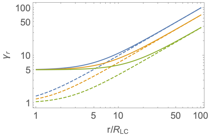
Figure 4: Lorentz factors corresponding to (18) compared with Michels’ solution $\gamma=\sqrt{1+r^{2}\Omega^{2}\sin^{2}\theta}$ for $\gamma_{0}=5$ and $\theta=\pi/8,\,\pi/4,\,\pi/2$ (bottom to top). Only at large distances $r\geq\gamma_{0}R_{LC}$ MHD acceleration picks up.

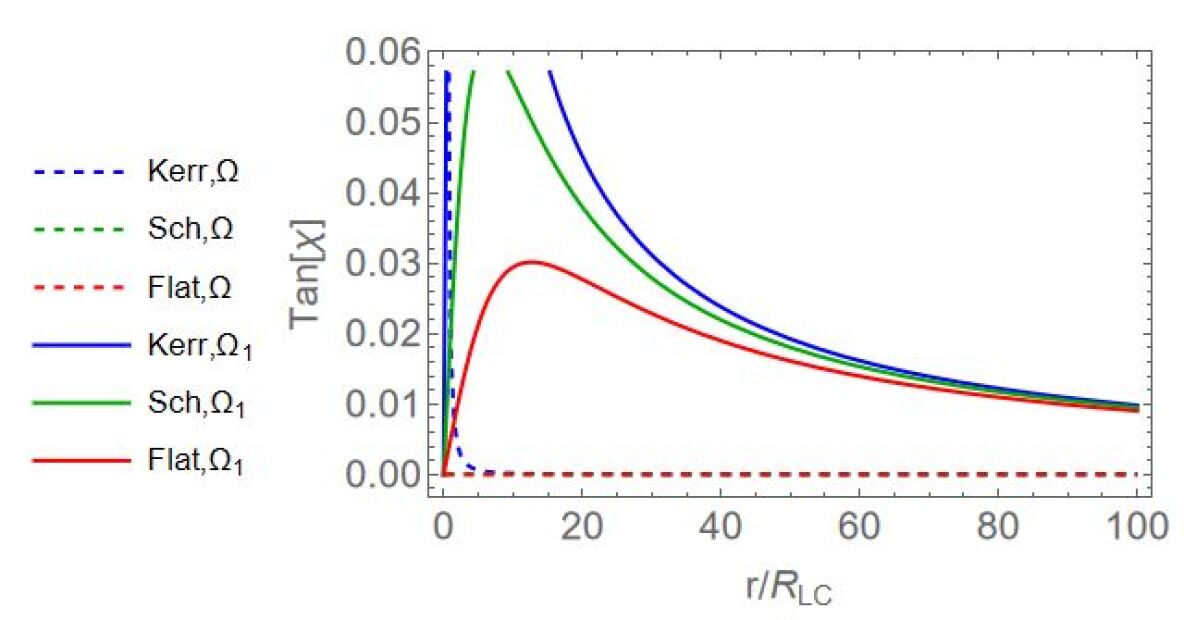
Figure 5: MODIFIED We see that they all coincide to zero by the LC; the Kerr case joins them to be zero too in some light cylinder radii.

It may be verified using Lorentz transformations that the electric field in the frame of the particle is zero.

The integration constant $\gamma_{0}$ physically corresponds to some value of the energy at some location. With a change of parameter $\gamma_{0}$, so that $\gamma_{0}+1/({2\gamma_{0}})\to\gamma_{LC}$, the solution would correspond to initial condition $\gamma_{LC}$ on the light cylinder:

$$\beta_{r}=\frac{1-\sin^{2}\theta r^{2}\Omega^{2}}{\frac{\gamma_{LC}+\sqrt{\gamma_{LC}^{2}-2}}{2\sqrt{\frac{1}{4}\left(\gamma_{LC}+\sqrt{\gamma_{LC}^{2}-2}\right){}^{2}+\sin^{2}\theta r^{2}\Omega^{2}-1}}-\sin^{2}\theta r^{2}\Omega^{2}}$$ (19)

In what follows we skip this unnecessary redefinition. Numerically $\gamma_{0}$ is typically very close to the energy of the particle crossing the outer light cylinder, see e.g. (17). Also, in appendix (E) we discuss the range of the allowed values for this constant of motion and we show that this constant behaves the same as the initial Lorentz factor of a particle at the outer light cylinder when $\gamma_{0}\gg 1$; hence, we give this constant the symbol $\gamma_{0}$.

ML: do we need this?

Relations (26) can also be derived from the geodesic equation for four-momenta $u_{0}$ and $u_{r}$ with Christoffel symbols (16). We find

$$\partial_{\tau}u_{0}=r\Omega^{2}\left(u_{r}+u_{0}\right)\left(r^{2}\Omega^{2}\left(u_{r}+u_{0}\right)+2u_{r}\right)\mbox{}$$

$$\partial_{\tau}u_{r}=-r\Omega^{2}\left(u_{r}+u_{0}\right)\left(r^{2}\Omega^{2}\left(u_{r}+u_{0}\right)+u_{r}-u_{0}\right)$$ (20)

Given Lagrangian (A1), with correctly chosen fixed value of the Lagrangian ${\cal{L}}=−1/2$ in affine parameterization (see 2018AmJPh..86..678P, for a brief related discussion), we find

$$\partial_{\tau}u_{r}=r\Omega^{2}$$ (21)

consistent with (26)

$$u_{0}=\partial_{\tau}t=\gamma\mbox{}$$

$$u_{r}=\gamma\partial_{t}r$$ (22)

$$r^{\prime\prime}(t)=\Omega^{2}r\left(1-r^{\prime}\right)\left(1+\left(\Omega^{2}r^{2}+2\right)r^{\prime 2}+r^{\prime}-\Omega^{2}r^{2}\right)\mbox{}$$

$$\gamma^{\prime}(t)=r\Omega^{2}\gamma(t)\left(1-r^{\prime}\right)\left(r^{2}\Omega^{2}-\left(r^{2}\Omega^{2}+2\right)r^{\prime}\right)$$ (23)

(First Integral?)

Importantly, toroidal component of the velocity always remains small

$$\beta_{\phi}=\sin\theta r\Omega(1-\beta_{r})=\frac{\gamma_{0}-\sqrt{\gamma_{0}^{2}+r^{2}\Omega^{2}\sin^{2}(\theta)-1}}{\gamma_{0}-r^{2}\Omega^{2}\sin^{2}(\theta)\sqrt{\gamma_{0}^{2}+r^{2}\Omega^{2}\sin^{2}(\theta)-1}}r\Omega\sin(\theta)$$ (24)

its maximal value is reached at $r\approx 1.27\gamma_{0}/\Omega$ and equals

$$\beta_{\phi,max}\approx 0.3/\gamma_{0}$$ (25)

The angle of motion with respect to the radial direction, $\tan\chi=\beta_{\phi}/\beta_{r}$ always remains small, Fig. 6

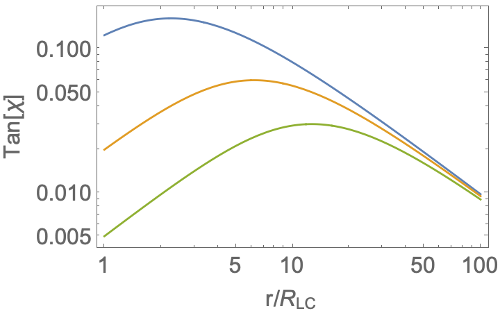
Figure 6: Angle of motion with respect to the radial direction, $\tan\chi=\beta_{\phi}/\beta_{r}$ for $\gamma_{0}=2,5,10$ (top to bottom); flat space $M=0$. The motion is nearly radial.

We also note simple relations in terms of proper time $\tau$ (for $\theta=\pi/2$).

$$\frac{dr}{d\tau}=\gamma\frac{dr}{dt}=\sqrt{\gamma_{0}^{2}+r^{2}\Omega^{2}-1}\mbox{}$$

$$\frac{d^{2}r}{d\tau^{2}}=r\Omega^{2}$$ (26)

Eq. (26) has a solution

$$\Omega r(\tau)=\gamma_{0}\sinh(\tau\Omega)+\cosh(\tau\Omega)\mbox{}$$

$$r^{\prime}(\tau)=\gamma_{0}\cosh(\tau\Omega)+\sinh(\tau\Omega)$$ (27)

(using $r(0)=1/\Omega$ and $r^{\prime}(0)=\gamma_{0}$). In proper time the Lorentz factor doubles approximately in $\tau\sim 1/\Omega$. This result is consistent with doubling in observer time in $t\sim\gamma_{0}/\Omega$, at distance $r\sim\gamma_{0}R_{LC}$

3.3 Schwarzschild black hole, $a=0$

Metric tensor is now

$$G_{00}=\alpha^{2}-\sin^{2}\theta r^{2}\Omega^{2}=G^{rr}\mbox{}$$

$$G_{0r}=-\sin^{2}\theta\frac{r^{2}\Omega^{2}}{\alpha^{2}}=G^{0r}\mbox{}$$

$$G_{rr}=\alpha^{-2}+\sin^{2}\theta\frac{r^{2}\Omega^{2}}{\alpha^{4}}=G^{00}\mbox{}$$

$$||G||=-1$$ (28)

(a factor of minus one is explicitly included in the definition of the 0-0 component of the metric).

The Christoffel symbols evaluate to

$$\Gamma^{0}_{00}=-\frac{\Omega^{2}\sin^{2}(\theta)\left(M-r^{3}\Omega^{2}\sin^{2}(\theta)\right)}{\alpha^{2}}\mbox{}$$

$$\Gamma^{0}_{0r}=-\frac{\left(r^{3}\Omega^{2}\sin^{2}(\theta)-M\right)\left(\alpha^{2}+r^{2}\Omega^{2}\sin^{2}(\theta)\right)}{\alpha^{4}r^{2}}\mbox{}$$

$$\Gamma^{0}_{rr}=\frac{\Omega^{2}\sin^{2}(\theta)\left(-5M+r^{3}\Omega^{2}\sin^{2}(\theta)+2r\right)}{\alpha^{6}}\mbox{}$$

$$\Gamma^{r}_{rr}=\frac{\Omega^{2}\sin^{2}(\theta)\left(-3M+r^{3}\Omega^{2}\sin^{2}(\theta)+r\right)}{\alpha^{4}}+\frac{2M^{2}}{r^{3}\alpha^{4}}-\frac{M}{\alpha^{4}r^{2}}\mbox{}$$

$$\Gamma^{r}_{0r}=\frac{\Omega^{2}\sin^{2}(\theta)\left(M-r^{3}\Omega^{2}\sin^{2}(\theta)\right)}{\alpha^{2}}\mbox{}$$

$$\Gamma^{r}_{00}=\frac{\left(r^{3}\Omega^{2}\sin^{2}(\theta)-M\right)\left(r^{3}\Omega^{2}\sin^{2}(\theta)-\alpha^{2}r\right)}{r^{3}}$$ (29)

COMMENT: INCORRECT: minus sign as well .. SEE EQUATION F44. Should be

$$\left(\beta_{r}=\alpha^{2}\frac{\alpha^{2}-\sin^{2}\theta r^{2}\Omega^{2}}{\pm\frac{\alpha^{2}\gamma_{0}}{\sqrt{\gamma_{0}^{2}+\sin^{2}\theta r^{2}\Omega^{2}-\alpha^{2}}}+\sin^{2}\theta r^{2}\Omega^{2}}\right)$$ (30)

The radial velocity now is

$$\beta_{r}=\alpha^{2}\frac{\alpha^{2}-\sin^{2}\theta r^{2}\Omega^{2}}{\frac{\alpha^{2}\gamma_{0}}{\sqrt{\gamma_{0}^{2}+\sin^{2}\theta r^{2}\Omega^{2}-\alpha^{2}}}-\sin^{2}\theta r^{2}\Omega^{2}}=\left\{\begin{array}[]{cc}\alpha^{2}\left(1-\frac{\alpha^{2}}{2\gamma_{0}^{2}}\right),&\gamma_{0}\gg r\Omega\sin\theta\\ \alpha^{2}\left(1-\frac{1}{\sin^{2}\theta r^{2}\Omega^{2}}+\frac{\gamma_{0}}{\alpha^{2}\sin^{3}\theta r^{3}\Omega^{3}}\right),&r\to\infty\end{array}\right.$$ (31)

Factors of $\alpha^{2}$ in front are just relativistic coordinate time dilation for a particle moving in gravitational field.

3.4 Kerr black hole

In the equatorial plane we find

$$\beta_{r}=\frac{\alpha\sqrt{\Delta}\Delta_{1}\left(r\left(\alpha^{2}-\Delta_{1}\Omega^{2}\right)-4aM^{2}\Omega\right)}{\gamma_{0}\sqrt{\frac{r\left(4a^{2}\Delta_{1}M^{4}r^{2}\left(\alpha^{2}+\Delta_{1}\Omega^{2}\right)-16a^{3}\Delta_{1}M^{6}r\Omega+16a^{4}M^{8}-8a\alpha^{2}\Delta_{1}^{2}M^{2}r^{3}\Omega+\alpha^{4}\Delta_{1}^{2}r^{4}\right)}{4aM^{2}\Omega+r\left(-\alpha^{2}+\gamma_{0}^{2}+\Delta_{1}\Omega^{2}\right)}}+4a^{2}M^{4}-\Delta_{1}^{2}r^{2}\Omega^{2}}$$ (32)

For $r\to\infty$ we find

$$\beta_{r}=\alpha^{2}-\frac{1-a^{2}M^{2}\Omega^{2}/2}{r^{2}\Omega^{2}}+\frac{\gamma_{0}+4M\Omega(1-aM\Omega/2)}{r^{3}\Omega^{3}}$$ (33)

It is understood that the solutions above involve both the kinematic effects of time-dilation (e.g. factor of $\alpha$ in front for the Schwarzschild case), as well as effects of centrifugal acceleration.

In conclusion, in all cases a particle moves radially with $\gamma\approx\gamma_{0}$ until $r\Omega\sim\gamma_{0}$. After that the wind acceleration takes over with $\gamma\sim r\Omega$.

3.5 Spiral with arbitrary radial step

The radial step of a magnetic spiral (denoted below $\equiv c/\Omega_{1}$) may be different from $c/\Omega$, e.g., the field may be affected by plasma inertia. For example, it is expected that inertial effects will make the spiral more tightly bound, larger $d\phi^{\prime}$ for a given $dr$, hence $\Omega_{1}\geq\Omega$. Equivalently, if the fast mode propagates with $\beta_{s}\leq 1$, in (3),

$$\beta_{F}\to\beta_{s}\beta_{F}\mbox{}$$

$$\Omega_{1}=\frac{\Omega}{\beta_{s}}\geq\Omega$$ (34)

Most importantly, the radial velocity of fast mode’s propagation may change with radius depending on local plasma parameters. In this case the shape of the spiral is non-Archimedean. In our notations this implies radial dependence of the radial step: $\Omega_{1}(r)$.

Corresponding relations are fairly compact in Schwarzschild metric. Using

$$d\phi\to d\phi^{\prime}-\Omega dt\mbox{}$$

$$d\phi^{\prime}\to-\frac{\Omega_{1}}{\alpha^{2}}dr$$ (35)

(instead of corresponding relations (5) with $\Omega_{1}=\Omega$), we find

$$\beta_{r}=\frac{\alpha^{2}\left(\alpha^{2}-r^{2}\Omega^{2}\right)}{\frac{\alpha\gamma_{0}\sqrt{\alpha^{2}+r^{2}\left(\Omega_{1}^{2}-\Omega^{2}\right)}}{\sqrt{-\alpha^{2}+\gamma_{0}^{2}+r^{2}\Omega^{2}}}-r^{2}\Omega\Omega_{1}}=\left\{\begin{array}[]{cc}\alpha^{2}\left(\frac{\alpha^{2}-r^{2}\Omega^{2}}{\alpha\sqrt{\alpha^{2}+r^{2}\left(\Omega_{1}^{2}-\Omega^{2}\right)}-r^{2}\Omega\Omega_{1}}\right),&\gamma_{0}\gg r\Omega\\ \alpha^{2}\left(\frac{\Omega}{\Omega_{1}}-\frac{\left(\Omega_{1}-\gamma_{0}\sqrt{\Omega_{1}^{2}-\Omega^{2}}\right)}{\alpha^{2}r^{2}\Omega_{1}^{2}\Omega}\right),&r\to\infty\end{array}\right.$$ (38)

For flat space

$$\beta_{r}=\frac{1-r^{2}\Omega^{2}}{\frac{\gamma_{0}\sqrt{1+r^{2}\left(\Omega_{1}^{2}-\Omega^{2}\right)}}{\sqrt{\gamma_{0}^{2}+r^{2}\Omega^{2}-1}}-r^{2}\Omega\Omega_{1}}=\left\{\begin{array}[]{cc}\frac{1-r^{2}\Omega^{2}}{\sqrt{1+r^{2}\left(\Omega_{1}^{2}-\Omega^{2}\right)}-r^{2}\Omega\Omega_{1}}\left(1-\frac{\left(1-r^{2}\Omega^{2}\right)\sqrt{r^{2}\left(\Omega_{1}^{2}-\Omega^{2}\right)+1}}{2\gamma_{0}^{2}\left(\sqrt{r^{2}\left(\Omega_{1}^{2}-\Omega^{2}\right)+1}-r^{2}\Omega\Omega_{1}\right)}\right),&\gamma_{0}\gg\Omega r\par\\ \frac{\Omega}{\Omega_{1}}-\frac{\left(\Omega_{1}-\gamma_{0}\sqrt{\Omega_{1}^{2}-\Omega^{2}}\right)}{r^{2}\Omega_{1}^{2}\Omega},&r\to\infty\end{array}\right.$$ (39)

Importantly, in the above relations the function $\Omega_{1}(r)$ is arbitrary, limited only by the condition $\Omega_{1}\geq\Omega$. (So that a radial step per rotation can be smaller or equal to the light cylinder.

For given $\Omega$ and $\Omega_{1}$ the toroidal velocity is

$$\beta_{\phi}=r\Omega\left(1-\frac{\Omega_{1}}{\Omega}\beta_{r}\right)$$ (40)

Note that here $\Omega_{1}$ may depend on radius $r$.

On physical grounds we expect $\Omega_{1}\approx\Omega$. In other words, fast mode is nearly relativistic and plasma is nearly force-free. This is the intrisic assumption of the model. For example, if $\Omega_{1}=(1+\delta_{\Omega})\Omega$, $\delta_{\Omega}\ll 1$, then

$$\beta_{\phi}=r\Omega(1-\beta_{r}+\delta_{\Omega})$$ (41)

Thus, for Archemedian spiral with the radial step $1/\Omega$, a particle slightly overtakes the rotation pattern with the rate $\sim r\Omega(1-\beta_{r})\ll r\Omega$, while for $1-\beta_{r}\ll\delta_{\Omega}$ a particle lags behind.

Thus, azimuthal velocity is small right from the light cylinder. Maximal toroidal velocity is $\sim 1/\gamma_{0}$, or $\sim\delta_{\Omega}$.

4 Numerical test

We have developed a Boris-based pusher (Boris & Roberts, 1969; Birdsall & Langdon, 1991). We verify the analytical results with direct integration, as we discuss below.

For Michel (1973) solution, consider a particle that in the wind frame (boosted by $\beta_{EM}$ from the lab frame) moves with Lorentz factor $\gamma_{0}^{\prime}$ (prime indicates Lorentz factor measured in the flow frame). Using electromagnetic velocity (1) and Lorentz transformations, we find the momentum in the lab frame $p_{\parallel}$

$$p_{\parallel}=\left\{\frac{\beta_{0}^{\prime}\gamma_{0}^{\prime}+\left(\gamma_{0}^{\prime}-1\right)r^{2}\sin^{2}\theta\Omega^{2}}{\sqrt{1+r^{2}\sin^{2}\theta\Omega^{2}}},0,\frac{\left(\sqrt{1-\beta_{0}^{\prime}}-\sqrt{\beta_{0}^{\prime}+1}\right)r\Omega\sin(\theta)}{\sqrt{\beta_{0}^{\prime}+1}\sqrt{1+r^{2}\Omega^{2}\sin^{2}(\theta)}}\right\}$$ (42)

The momentum $p_{\parallel}$ is that of a particle that is sliding along the local magnetic field with Lorentz factor $\gamma_{0}^{\prime}$ as measured in the frame associated with $\beta_{EM}$ (where electric field is zero). This is not a radial dependence, only a transformation at a given radius.

The total Lorentz factor is

$$\gamma=\gamma_{0}^{\prime}\sqrt{1+\sin^{2}\theta r^{2}\Omega^{2}}=\sqrt{2}\gamma_{0}^{\prime}$$ (43)

a combination of parallel motion and orthogonal E-cross-B drift. The final relation in (43) applies to the light cylinder.

In Fig.4 we compare analytical results (18), and numerical integration - they are in excellent agreement.

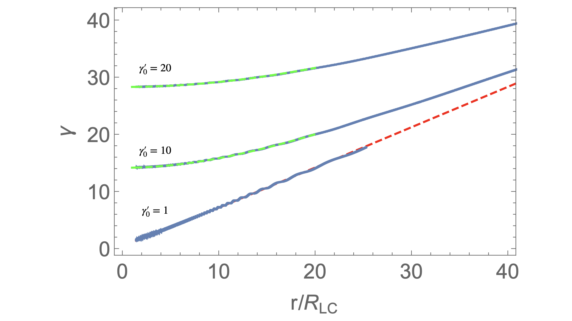
Figure 7: Direct integration of particle trajectories for the Lorentz factor of parallel motion $\gamma_{0}^{\prime}=1,\,10,\,20$, $\theta=\pi/4$ (solid lines). The $\gamma_{0}^{\prime}=1$ reproduces Michel’s solution $\gamma=\sqrt{1+r^{2}/2}$ (red dashed line). Green dashed lines: analytical solutions (18). In the simulations the magnetic field at the light cylinder satisfies $\omega_{B}=10^{4}\Omega$.

5 Wind acceleration by rotating magnetospheres

5.1 General comments

Our results have important implications for launching of winds and jets from pulsars and black holes (via Blandford & Znajek, 1977, mechanism in the latter case).

Three important ingredients of astrophysical relativistic jets are: (i) large bulk Lorentz factors; (ii) large total power; (iii) collimation. In the classical picture of jets, acceleration, total power and collimation are intrinsically connected (a single acronym ACZ: Acceleration and Collimation Zone, is often used, Blandford et al., 2019). For relativistic jets this creates a problem: the confining hoop stresses are nearly compensated by the electric force; so that the acceleration occurs on exceedingly long range of scales (1989ApJ...347.1055H; 2009ApJ...698.1570L).

We argue that acceleration-collimation-power of astrophysical jets are not as coupled as advocated, e.g., by the ACZ approach. Let us discuss the three ingredients separately.

5.2 Jet/wind acceleration

Both in pulsars (GJ) and black holes  (in the case of Blandford & Znajek, 1977, mechanism) the wind/jets are composed of pair plasma produced within the magnetosphere. It is expected that the newly born pairs are moving relativistically. This is especially true for the pairs produced by the curvature photons near pulsar polar caps (RS75; 1977ApJ...217..227F; 1982ApJ...252..337D), where the resulting pairs move with $\gamma_{0}\sim 10^{4}-10^{5}$ (2010MNRAS.408.2092T; 2013MNRAS.429...20T). High injection Lorentz factors are also expected in the case of two-photon pair production in pulsar outer gaps/ current sheet (e.g. 2000ApJ...537..964C; 2002ApJ...581..451A), since the collision typically involves photons or highly different energies. Qualitatively, the pair is produced with $\gamma_{e^{\pm}}\sim\sqrt{\epsilon_{high}/\epsilon_{low}}$, expected to be in the thousands. Though pairs are expected to be produced with arbitrary angles with respect to the local magnetic field, synchrotron decay will reduce perpendicular component, leaving large parallel momentum.

Our results demonstrate that initial acceleration of the magnetosphere-produced winds and jets (pair-dominated, loaded by the vacuum break-down within the magnetospheres) is independent of the global flow collimation: until large distances the initial Lorentz factor of the particles is the initial injection Lorentz factor $\gamma_{0}$.

Thus, both in pulsars and in black holes the initial Lorentz factor of flows originating from within the magnetosphere is $\gamma_{0}\gg 1$. This changes the acceleration/collimation paradigm: there is actually no need to accelerate the flow: it is moving relativistically fast from the start. In fact, in case of AGNe jets with typical Lorentz factors $\sim$ tens, the flow needs to be slowed down.

5.3 Jet/wind power

The power injected in the wind in the form of relativistic particles depends on (i) overall angular extent of the pair production region; (ii) a voltage drop along the magnetic field  within the pair production region.

Let us first discuss the geometry of the pair production region. Both in neutron stars and black holes the pair production is expected to occur: (i) on the majority of open fields lines, either at null points, or regions where Goldreich-Julian density $\rho_{GJ}$ vanishes; (ii) at the equatorial reconnection current sheet, Fig 8.

Pair production at $\rho_{GJ}=0$ is somewhat similar to the case of pulsar magnetospheres, (RS75; 1977ApJ...217..227F; 2010MNRAS.408.2092T; Chen & Beloborodov, 2014; 2018ApJ...855...94P; 2022ApJ...939...42H), also applied to BHs, e.g., by Ptitsyna & Neronov (2016). An advantage of dissipation/pair production at the null point or the surface $\rho_{GJ}=0$ is that it occurs on most of the magnetic field lines.

A number of authors discussed dissipation, and powering of the jet from the reconnection current sheet (Comisso & Asenjo, 2021; 2022ApJ...937L..34K; Ripperda et al., 2022). Though a possibility of reconnection-driven jets and flares looks appealing, it is expected that only a small fraction of field lines participate in the reconnection within the light cylinders - this reduces the total dissipated power.

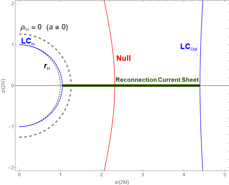
Figure 8: Semi-qualitative structure of BH magnetosphere. Inner and outer light cylinders are plotted for magnetic monopole field (i.e., radial flux surfaces) with angular velocity of field lines $\Omega=0.1$ for Schwarzschild black hole. Dashed black curve $r_{H}$ is the Schwarzschild horizon; blue curves are the inner $LC_{\rm in}$ and outer $LC_{\rm out}$ light cylinders; red curve is the null surface, Eq. (47). Dashed gray curve is $\rho_{GJ}=0$ surface in non-Schwarzschild case (i.e, $a\neq 0$, for the particular optimal choice of parameter (Beskin et al., 1992)). The horizontal green line that lies between the two light cylinders represents the surface of the reconnection current sheet.

In the case of black hole a self-consistent analysis can be done for rotating magnetospheres in Schwarzschild geometry and for Kerr metric in the equatorial plane. Generally there are two light cylinders - inner and outer ones, located at $G_{00}=0$.

For Schwarzschild geometry the light cylinders are at

$$\frac{2M}{r}+r^{2}\Omega^{2}\sin^{2}\theta=1$$ (44)

Plasma must be produced within the magnetosphere, somewhere between the light cylinders. Possible locations include the null points, which separate particles that, if initially stationary, will escape through the outer or inner light cylinder. In other words, a particle in radial magnetic field left along the null line is in (unstable) equilibrium. Therefore, the null line is where both the first and second derivatives of the radial coordinate of the particle vanish (classically speaking, we are looking for the points where the gravitational attraction balances the centrifugal repulsion; so, the radial acceleration and the radial speed must vanish there). From equation (B17), provided that the null line exists between the two light cylinders at $r=r_{0}$, we get

$$\ddot{r}(r_{0})=0\hskip 28.45274pt\xrightarrow[G_{00}(r_{0})=E^{2}]{\dot{r}(r_{0})=0}\hskip 28.45274pt\partial_{r}G_{00}(r_{0})=0\hskip 28.45274pt$$ (45)

Interestingly, both the locations of the light cylinders and the null line depend only on the metric component $G_{00}$. Thus, since $G_{00}$ has no information about the shape of the wire where the particle moves along (here, a spiral), the three locations we obtained are independent of that too. For Schwarzschild case, see Fig. 8,

$$r_{0}={M^{1/3}{\Omega^{-2/3}}\sin^{-{2}/{3}}\theta},$$ (47)

The null line for Kerr metric in the equatorial plane is

$$r_{0}=M\eta^{-\frac{2}{3}}(1-a\eta)^{\frac{2}{3}}\mbox{}$$

$$\eta=\Omega M$$ (48)

Alternatively, pairs within the black hole magnetosphere can be produced in gap regions, where the equivalent of the GJ vanishes. Pair production at the black hole analogues of pulsar outer gaps has been considered by Beskin et al. (1992); Beskin & Kuznetsova (2000). They found that for slowly rotating Kerr black hole, the condition $\rho_{GJ}=0$ is satisfied at $r=2^{1/3}\times 2M$.

Additional pair production will occur at the equatorial current sheet (Comisso & Asenjo, 2021). But since only a small number of corresponding flux tubes will cross the outer light cylinder, we expect that the contribution of the current sheet will be small if compared with more extended regions of pair production.

In conclusion, regardless of whether pairs are produced at the null surface, or the analogue of the outer gaps, pair production occurs on most (or even on all) magnetic field lines.

COMMENT: (REMOVE LATER IF IT IS CORRECT)

(SURFACE) GJ DENSITY [$\rho_{GJ}=0$] FOR MONOPOLAR FIELD

From Beskin (2009) and (Beskin et al., 1992), and for the case of Schwarzschild ($\omega=0$ and $\alpha=\sqrt{1-2M/r}$),

$$\rho_{GJ}=0\iff\vec{\nabla}\cdot\left(\frac{\Omega-\omega}{2\pi\alpha}\vec{\nabla}\Psi\right)=0\Rightarrow\vec{\nabla}\cdot\left(\frac{\vec{\nabla}\Psi}{\alpha}\right)=0$$ (49)

The magnetic flux has to be spherically symmetric, i.e., $\Psi:=\Psi(r,\theta)$; so, in the Schwarzschild metric (in normalized basis), we have

$$\vec{\nabla}\Psi(r,\theta)=\left\{\frac{\partial_{r}\Psi}{\sqrt{g_{rr}}},\frac{\partial_{\theta}\Psi}{\sqrt{g_{\theta\theta}}}\right\}=\left\{\frac{\partial_{r}\Psi}{\alpha},\frac{\partial_{\theta}\Psi}{r}\right\}$$ (50)

Define the following vector

$$\vec{V}=\frac{\vec{\nabla}\Psi}{\alpha}\hskip 14.22636pt\Rightarrow\hskip 14.22636pt\vec{V}=\left\{\frac{\partial_{r}\Psi}{\alpha^{2}},\frac{\partial_{\theta}\Psi}{r\alpha}\right\}$$ (51)

We obtain

$$\vec{\nabla}\cdot\vec{V}=\nabla_{\mu}V^{\mu}=\frac{1}{\sqrt{-g}}\partial_{\mu}\left(\sqrt{-g}V^{\mu}\right)=\left(\frac{2}{r}+\partial_{r}\right)V^{r}+\left(\frac{\cot{\theta}+\partial_{\theta}}{r}\right)V^{\theta}$$ (52)

For a monopole magnetic field Beskin (2009), we have (CITE: The structure of black hole magnetospheres ± I. Schwarzschild black holes)

$$\Psi(\theta)\propto(a+b\cos{\theta})\hskip 14.22636pt\Rightarrow\hskip 14.22636pt\vec{\nabla}\Psi(\theta)\propto\sin{\theta}\>e^{\theta}$$ (53)

$$\rho_{GJ}=0\iff\vec{\nabla}\cdot\vec{V}=0\iff$$ (54)

For a different flux,

$$\Psi(r)\propto r^{3}\Rightarrow\rho_{GJ}=0\iff r=\frac{9}{4}M$$ (55)

We note that it is independent of the rotation parameter of the field lines.

COMMENT: END COMMENT

Both in cases of neutron star and black hole magnetospheres pair formation occurs on most open field lines. The pair luminosity then can be estimated as as a parallel potential drop

$$L_{p}\sim\frac{1}{\sigma}L_{EM}\mbox{}$$

$$L_{EM}\sim\left\{\begin{array}[]{cc}B_{NS}^{2}R_{NS}^{2}c\left(\frac{\Omega R_{NS}}{c}\right)^{4},&\mbox{for neutron star}\\ ka^{2}B_{BH}^{2}R_{BH}^{2}c&\mbox{for {black hole}}\end{array}\right.$$ (58)

where $k\leq 1$ is some coefficient (Beskin & Kuznetsova, 2000).

The flow magnetization can be estimated as

$$\sigma\sim\frac{V_{tot}}{\Delta V}\mbox{}$$

$$V_{tot}\sim\left\{\begin{array}[]{cc}B_{NS}R_{NS}\left(\frac{\Omega R_{NS}}{c}\right)^{2},&\mbox{for neutron star}\\ aB_{BH}R_{BH}&\mbox{for {black hole}}\end{array}\right.$$ (61)

($V_{tot}$ is the total available potential, $\Delta V$ is a potential drop within the pair production region.

It is expected that $\sigma\gg 1$, hence the particle flux is small. Still, that small energy flux is carried by particles moving nearly radially with highly relativistic velocities.

6 Jet in M87

6.1 Particle dynamics in parabolic magnetic field

In our model collimation is completely separated from acceleration in the vicinity of the light cylinder. To demonstrate this, let’s choose prescribed collimated flow along parabolic flux surfaces

$$r(1-\cos\theta)={\rm const}$$ (62)

In this case it is more convenient to work in cylindrical coordinates. The flux surface is then given by

$$z=\frac{\varpi^{2}-r^{2}_{0}}{2r_{0}}$$ (63)

($\varpi$ is a cylindrical radial coordinate, $r_{0}$ is a parameter that marks a particular flux surface).

In the metric tensor we first change to the rotating frame, $d\phi\to d\phi^{\prime}-\Omega dt$, add parabolic constraint $dz\to(\varpi/r_{0})d\varpi$, and add a spiral step

$$d\phi^{\prime}=\Omega dl\mbox{}$$

$$dl=\sqrt{1+\varpi^{2}/r_{0}^{2}}d\varpi$$ (64)

At each location the velocity in $\{\varpi,\phi,z\}$ coordinates is

$$\left\{\beta_{\varpi},\Omega\varpi\left(1-\sqrt{1+\frac{\varpi^{2}}{\varpi_{0}^{2}}}\beta_{\varpi}\right),\frac{\varpi\beta_{\varpi}}{\varpi_{0}}\right\}$$ (65)

Metric tensor in this case

$$G_{00}=1-\Omega^{2}\varpi^{2}\mbox{}$$

$$G_{0\varpi}=\Omega^{2}\varpi^{2}\sqrt{1+\frac{\varpi^{2}}{\varpi_{0}^{2}}}\mbox{}$$

$$G_{\varpi\varpi}=\left(1+\frac{\varpi^{2}}{\varpi_{0}^{2}}\right)\Omega^{2}\varpi^{2}$$ (66)

Following our procedure we find

$$\beta_{\varpi}=\frac{1-\left(2\varpi-r_{0}\right)r_{0}\Omega^{2}}{\frac{\gamma_{0}}{\sqrt{\frac{\left(2\varpi-r_{0}\right)\left(\gamma_{0}^{2}+\left(2\varpi-r_{0}\right)r_{0}\Omega^{2}-1\right)}{\left(2\varpi-r_{0}\right)r_{0}^{2}\Omega^{2}-2\varpi}}}-\left(2\varpi-r_{0}\right)r_{0}\Omega^{2}}$$ (67)

The resulting acceleration differs little from the case of conical flux surfaces of the Michel (1973) solution, Fig. 9

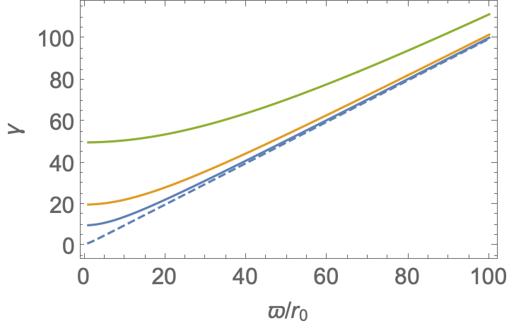
Figure 9: Lorentz factors of particles moving along parabolic spiral for different $\gamma_{0}=10,20,50$ (bottom to top curves). Dashed line is the Michel (1973) solution.

6.2 Emission maps

As we demonstrated above, particles injected from the black hole magnetosphere stream nearly along the magnetic flux surfaces - either conical for monopolar fields, parabolically, or more generally, along any given flux surface. The toroidal velocity remains small.

For a given shape of the magnetic flux surface (and some prescription for emissivity) we can then calculate the expected emission map. For monopolar magnetosphere any emission by relativistic radially moving particles will be centered on the source, the black hole.

Even for curved flux surfaces, particles move with constant Lorentz factor almost purely along the flux surfaces, with minimal $v_{\phi}$. For high injection Lorentz factors the emission will be dominated by the flow points when particle motion is aligned with the line of sight.

For example, for parabolical flux surfaces (Blandford & Znajek, 1977), also Eq. (62), neglecting GR contribution, the line of sight can be parallel to a given flux surface emanating from the magnetosphere only if the lone of sight is $\theta_{ob}\leq\pi/4$. For smaller $\theta_{ob}$, for a given flux surface parameterized by $r_{0}$ the tangent point is

$$\varpi_{t}=r_{0}\cot\theta_{ob}\mbox{}$$

$$z_{t}=(\cot^{2}\theta_{ob}-1)\frac{r_{0}}{2}$$ (68)

Choosing axis $x_{s}$ on the plane of the sky along the projection of the spin of the black hole on the plane of the sky, the tangent point projects to

$$x_{s}=\frac{r_{0}}{2\sin\theta_{ob}}\mbox{}$$

$$y_{s}=0$$ (69)

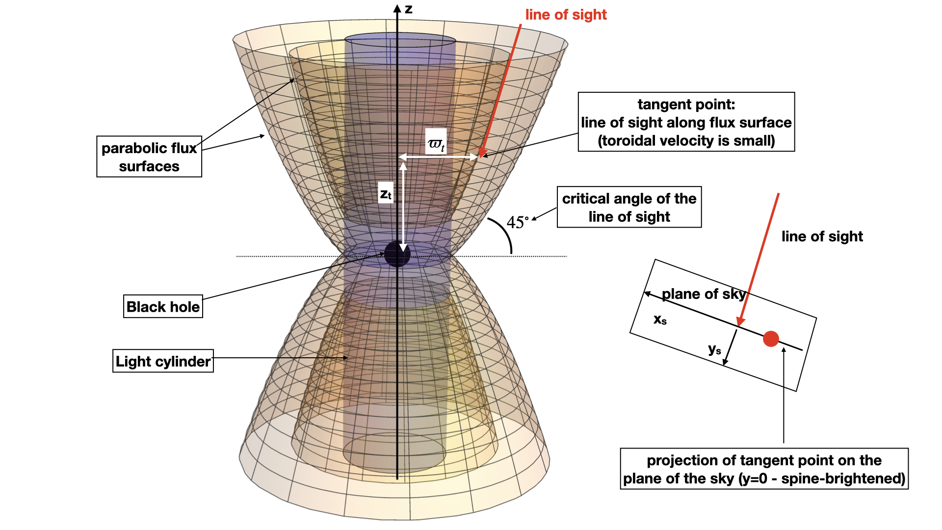
Figure 10: 3D rendering of parabolic magnetosphere. The vertical cylinder is the light cylinder. The insert on the right shows the sky image for a particular chosen line of sight. Due to high Doppler boosting the brightness peaks on the $y$ axis - the spine.

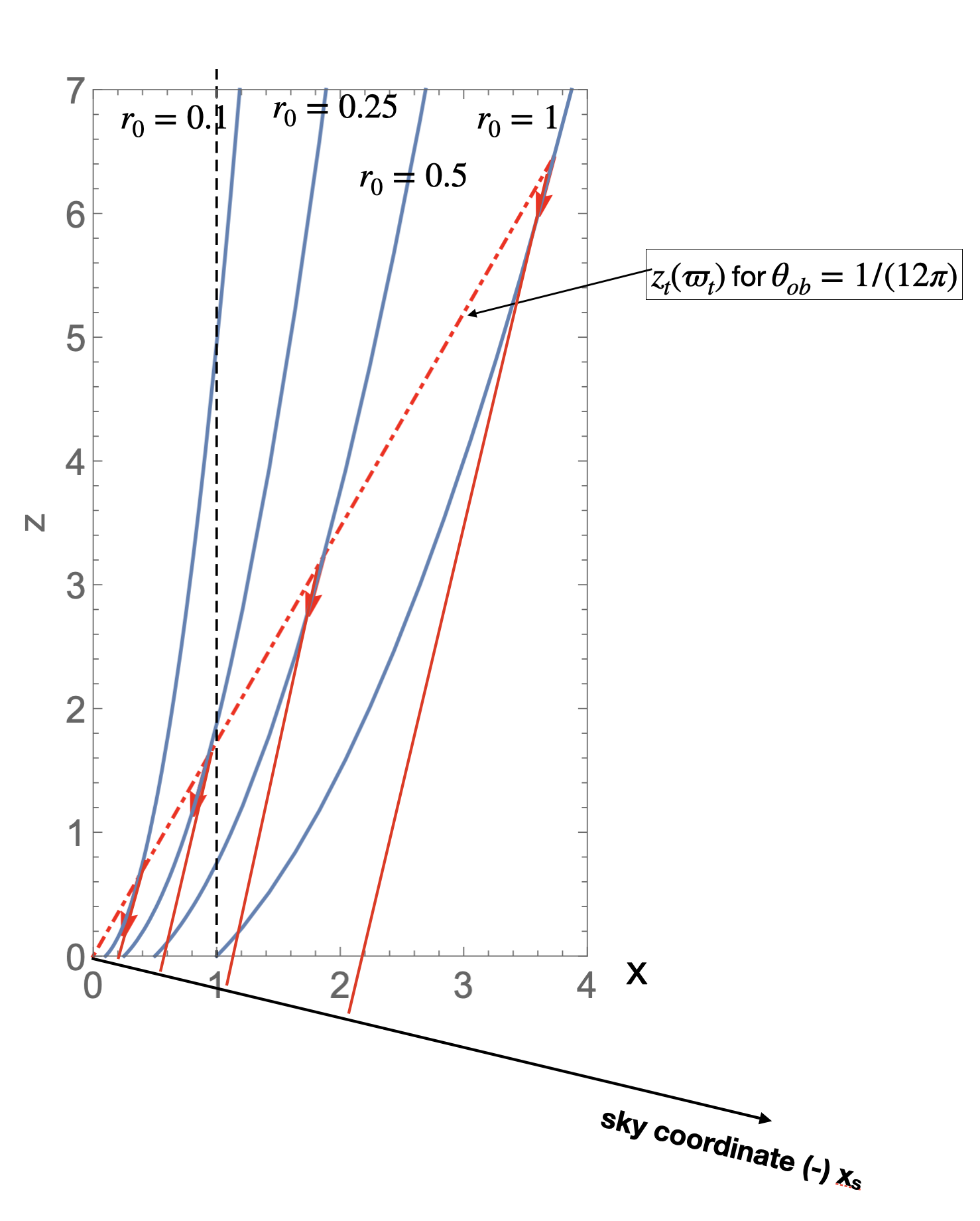
Figure 11: Parabolic magnetosphere and the lines of sight, $x-z$ cut. Solid lines are magnetic flux surface for $r_{0}=0.1,\,0.25,\,0.5,\,1$. Red arrows start at points where the local line of sight is along the flux surface (hence maximal Doppler factor). Red dashed line, Eq. (69) - location of all such points. In this example $\theta_{ob}=\pi/12$. Coordinates are normalized to light cylinder radius.

Since the observed pattern is dominated by Lorentz boost, to calculate the images we employ the following procedure:

• Given the velocity (65-67) we calculate local Doppler factor $\delta$. In fact, since toroidal velocity is small, one can use just the shape of the flux surface to find the local direction of the flow.

• We scale local density (somewhat arbitrary) as $1/r^{2}$, total spherical distance to the black hole.

• local emissivity is parameterized as

  $$j\propto\frac{\delta^{3}}{r^{2}}$$ (70)

• emissivity is integrated along the line of sight.

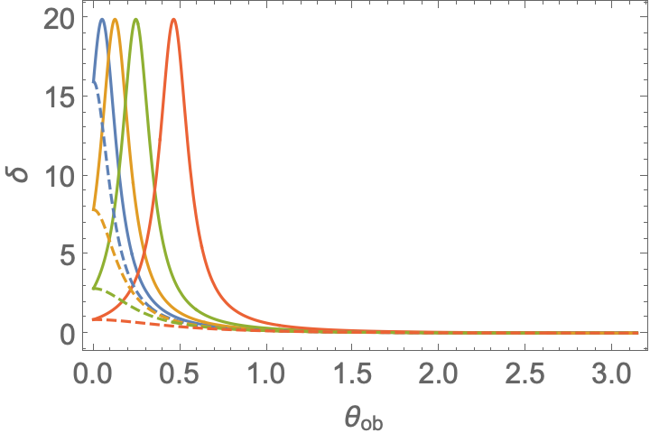
Figure 12: Doppler factor as a function of the observer angle $\theta_{ob}$ at $r=2$. Slices are in the line-of-sight-black hole spin plane (solid lines) and in the orthogonal plane (dashed lines). Peaks in $\delta$ correspond to angles when the line-of-sight is tangential to the flux surface. Here and for the images below $\gamma_{0}=10$.

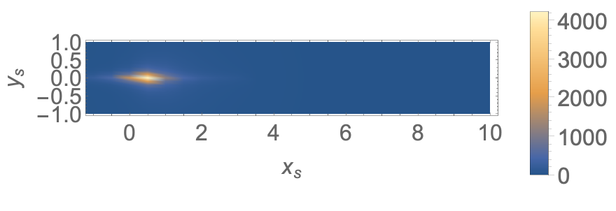
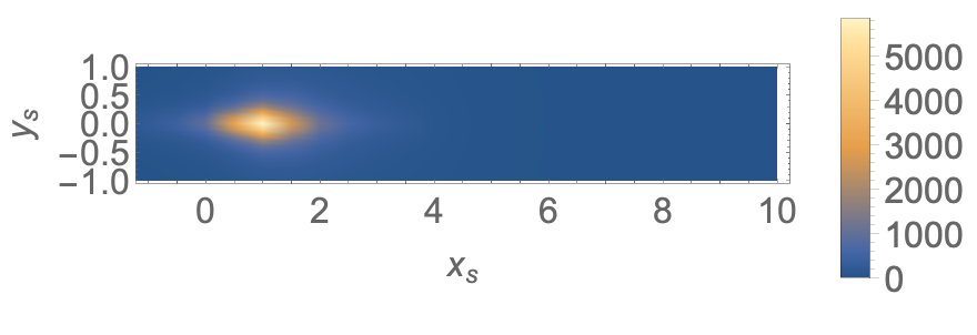
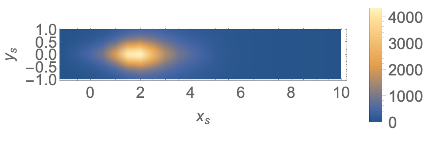
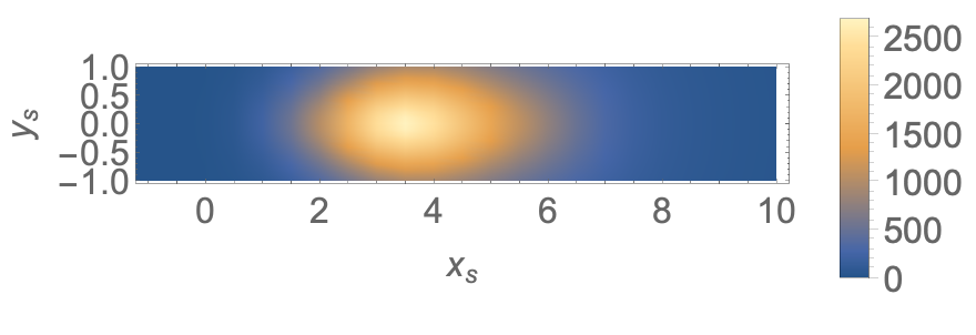
Figure 13: Image maps for $r_{0}=0.1,\,0.25,\,0.5,\,1$, $\theta_{ob}=\pi/12$. The axes correspond to projected distances measured in terms of the light cylinder radius.

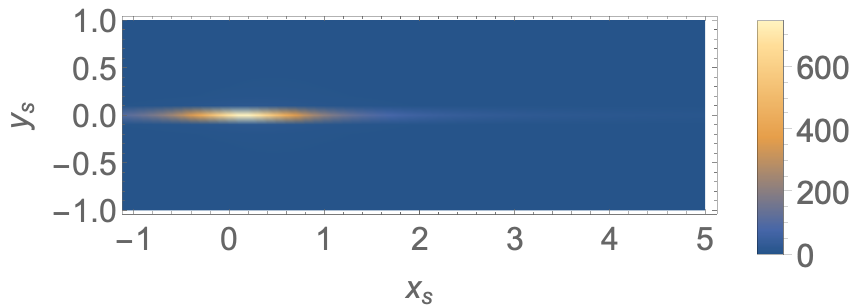
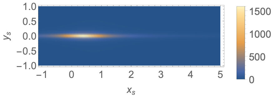
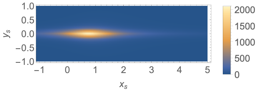
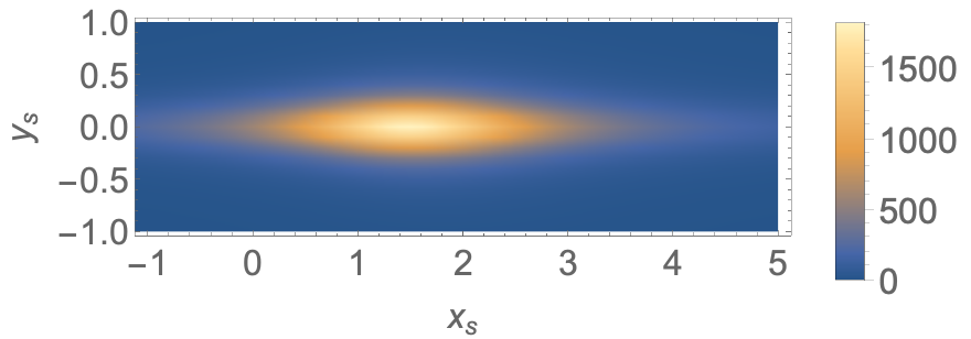
Figure 14: Image maps for $r_{0}=0.1,\,0.25,\,0.5,\,1$, $\theta_{ob}=\pi/6$.

In Fig. 12 we plot slices of the Doppler factor in the two orthogonal planes. Expected brightness maps are plotted in Figs. 13-15. All images, for any surface parameter $r_{0}$, are spine-brightened. Hence any combination will be spine-brightened as well.

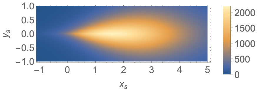
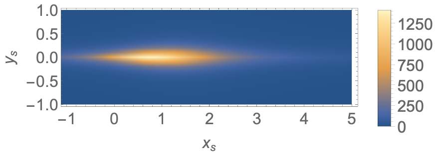
Figure 15: Image maps integrated over $0\leq r_{0}\leq 1$ for $\theta_{ob}=\pi/12$ (top panel) and $\theta_{ob}=\pi/6$ (bottom panel). Larger $r_{0}$ corresponds to flux surfaces not emanating from the magnetosphere.

Finally, we conciliate emission from a possible current sheet outside of the light cylinder (Comisso & Asenjo, 2021), by integrating the flux parameter $r_{0}$ from $1$ to $2$. The resulting structure is more elongated, more extended sideways, but is still spine-brightened, Fig. 16.

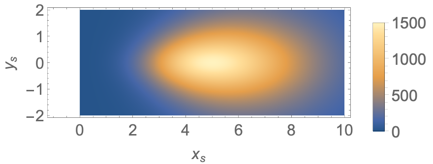
Figure 16: Emission pattern from the outside current sheet, $1\leq r_{0}\leq 2$

6.3 Conclusion: morphology of M87 jet and the BZ mechanism

Our results show a universal property of the resolved Blandford & Znajek (1977) flow with large parallel (to the local magnetic field) momentum of emitting particles: all images are spine-brightened, agreeing with what was observed. No special prescription for emissivity as function of the flux function parameter $r_{0}$ can change that: they are all spine-brightened. The assumption of parabolical flux surfaces is, naturally, an analytic approximation, yet the universality of the result - spine-brightened profile - ensures that it will be applicable to more general cases.

We then conclude that Blandford & Znajek (1977) mechanism is responsible for the M87 jet, at least in its pure form. By BZ mechanism we understand generation of collimated relativistic jet. The relativistic $e^{\pm}$ we describe do extract energy from the spin of the black hole.

The Blandford & Znajek (1977) mechanism can still be operational - and, e.g. responsible for the bright core in the images of M87 in case of purely radial outflow at small $r$, but it does not drive the observed jet. Another possibility is that the sheath is slowed down by the interaction with the disk corona - while the core remains relativistic, with emission beamed away. This would correspond to emission coming only from small $r_{0}$, top rows in Figs. 13 and 14 - it is still spine-brightened, but shows only in the small part of the image.

In contrast disk-produced outflows (Blandford & Payne, 1982) start non-relativistically. The extended structure observed in M87 is thus inconsistent with the magnetosphere-produced jet, but is consistent with the disk-produce jets.

On larger scales, of the order of parsecs, in the grand spiral paradigm of a jet moving with Lorentz factor of $\sim$ few Lyutikov et al. (2005), the edge-brightened jet is actually expected on theoretical grounds (e.g. Fig. 1 of Clausen-Brown et al., 2011). In addition, asymmetries across the jet in intensity, polarization and spectral index maps are expected.

6.4 Variability and very high energy emission from non-blazar AGNe

The observation of rapidly variable very high energy (VHE) gamma-rays from non-aligned active galactic nuclei (AGNs), e.g., from M87 and Cen A, proves challenging for conventional theoretical acceleration and emission models (1996Natur.383..319G; 2006Sci...314.1424A; 2007ApJ...664L..71A; 2008ApJ...679..397A; 2008A&A...479L...5R; 2009ApJ...695L..40A). Even for the jet-aligned Blazers variations down to a few minutes time scale, smaller than the expected size of the black hole (2005A&A...442..895A), are difficult to explain (2009Ap&SS.321...57I).

The present model provides a possible answer, Fig. 8: (i) particles are streaming relativistically, radially and quasi-isotropically right in the vicinity of the black hole. One may expect that the variability is related to the thickness of the acceleration region, either at null points or at the surface $\rho_{GJ}=0$. The corresponding thickness is much smaller that $R_{BH}$.

As the particles propagate further out in an environment changing on scales $\sim 1/\Omega_{BH}$, then the typical time scale of variability $t_{var}$ is

$$t_{var}\sim(c/\Omega_{BH})\times 1/\gamma_{0}^{2}=a_{Kerr}^{-1}\times R_{BH}/c\times 1/\gamma_{0}^{2}$$ (71)

where $a_{Kerr}$ is the Kerr spin parameter and $R_{BH}$ is the horizon size of the black hole. Since the expected Lorentz factor $\gamma_{0}$ can be in the thousands, the variability time scale can be very short.

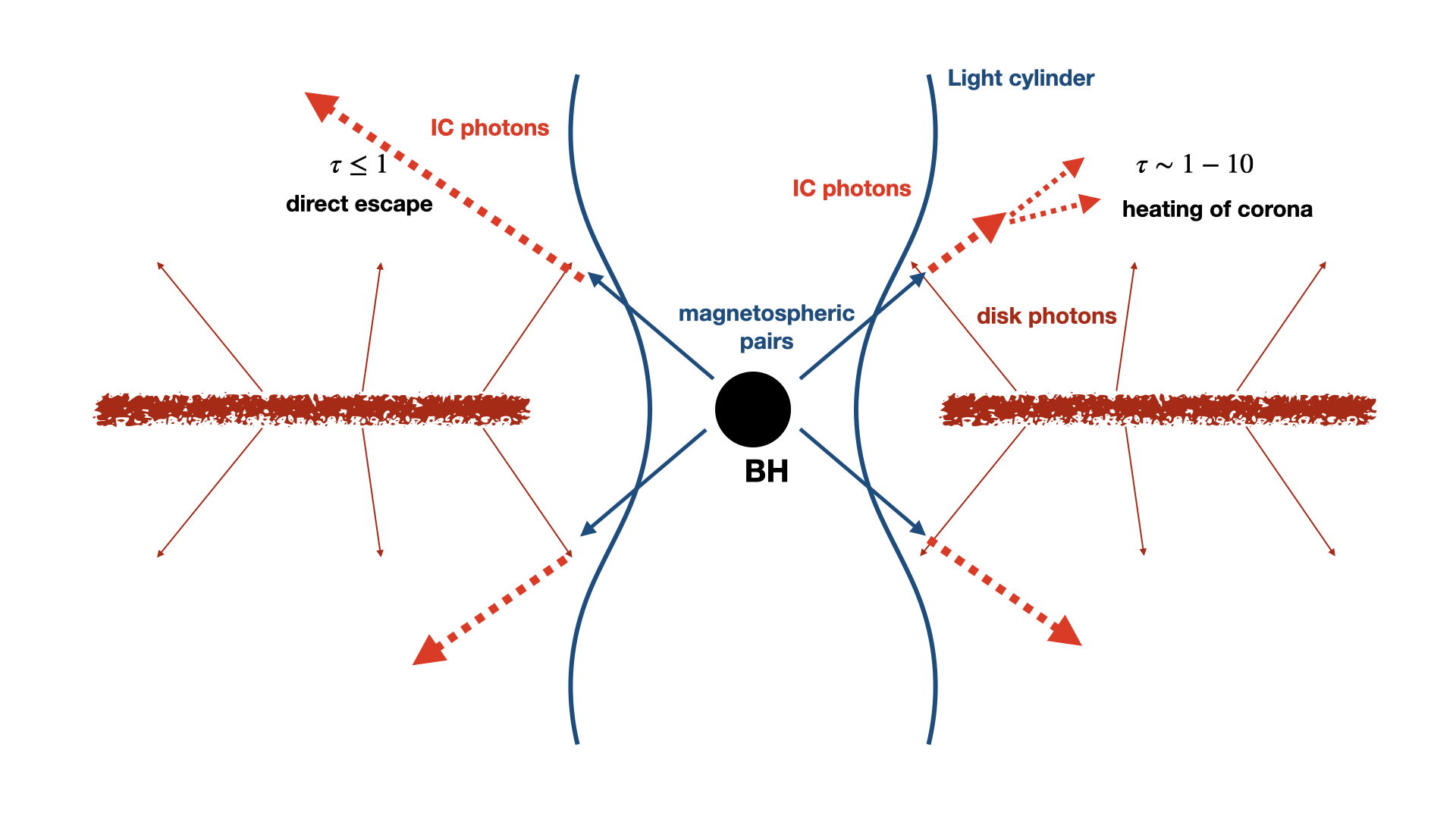
Figure 17: Cartoon of the IC emission by accreting black hole. Particles accelerated with the black hole magnetosphere  to $\gamma_{0}\gg 1$ IC scatter the soft photons from the disk. The resulting signal is (i) quasi-isotropic; (ii) highly variable due to temporal variations of the gap-produced particle flux.

With respect to the high energy emission, as a rough estimate of the IC luminosity by particles accelerated with the black hole magnetosphere on the disk photons, one can assume that the disk luminosity is a fraction $\eta_{ph}$ of Eddington luminosity, $L=\eta_{ph}L_{E}$. The local photon energy density is then

$$u_{ph}=\eta_{ph}u_{Edd}\mbox{}$$

$$u_{Edd}=\frac{L_{E}}{4\pi R_{BH}^{2}c}$$ (72)

The IC power emitted by each particle can be estimated as

$$l_{IC}=\gamma_{0}^{2}\sigma_{T}cu_{ph}$$ (73)

A possible way to estimate the number of emitting particle is to scale particle flux to the total jet flux $L_{j}$ using magnetization parameter $\sigma$

$$4\pi R_{BH}^{2}\gamma_{0}nm_{e}c^{3}\sim\frac{L_{j}}{\sigma}$$ (74)

Combining the above estimates the the IC luminosity evaluates to

$$\frac{L_{IC}}{L_{jet}}\approx\gamma_{0}\frac{m_{p}}{m_{e}}\times\frac{\eta_{ph}}{\sigma}$$ (75)

Though the estimate (75) is sensitive to the assumed parameters, it shows that large, quasi-isotropic IC luminosity may be produced.

In the case of M87, the disk luminosity is highly sub-Eddington, $L_{disk}\sim 10^{42}$ erg s^-1, $L_{Edd}\sim 4\times 10^{47}$ erg s^-1 (e.g. 1996MNRAS.283L.111R), so $\eta_{ph}\sim 2\times 10^{-6}$. Jet luminosity is $L_{jet}\sim 10^{43}$ erg s^-1. For $\gamma_{0}\sim\sigma$ the expected IC luminosity is low, $\sim 10^{40}$ erg s^-1.

We leave investigation of the corresponding radiative properties (e.g. escape of the very high energy photons) to a separate investigation.

6.5 Radio galaxy PBC J2333.9-2343 with a blazar-like core

2023arXiv230308842H discuss an interesting case of a giant radio galaxy, with jets apparently at large angle to the line of sight, yet with blazar-like core, Fig. 18. The core shows many features characteristic of a blazar - high energy emission and short time scale variability across the spectrum.

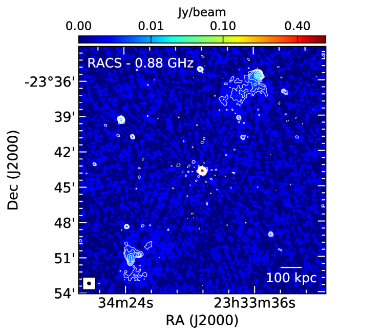
Figure 18: Image of PBC J2333.9-2343 from the RACS survey at 0.88 GHz. Morphology of lobes implies large angle between jet direction and the line of sight. The core shows many features of a blazar (2023arXiv230308842H).

Our interpretation is that in this case we are directly observing inner parts of the flow, left part of the cartoon in Fig. 17, which are relativistic and produce blazar-like phenomena. This, we suggest, became possible due to variations of the disk parameters, e.g. lighter disk with more transparent corona.

6.6 Plasma dynamics and pair production in force-free and PIC simulations

Two approaches are commonly used to study relativistic winds and jets: force-free simulation (Spitkovsky, 2006, e.g.) and PIC simulations (e.g. Chen & Beloborodov, 2014; Philippov et al., 2015; Crinquand et al., 2020; Hakobyan et al., 2022; Ripperda et al., 2022).

In ideal force-free simulation the velocity along the field is not defined in principle. (Inclusion of resistivity in the force-free approach requires some choice of parallel velocity Lyutikov (2003); Gruzinov (2007).) Thus the effects discussed here are completely missed in force-free simulation.

In case of PICs the effects of initial large injection Lorentz factor are missed by choice (see though Crinquand et al., 2020). To simulate pair production in PICs typically some kind of prescription is employed: either a density floor, or a condition on the value of the local electric field. Acceding to a given prescription pairs are added at rest (except in Crinquand et al., 2020). Instead, they should be added with large Lorentz factors. If the number of added pairs is comparable to the initial one, the resulting structure of the magnetosphere will be drastically different.

Our results have implications for PIC simulations (that the newly born $e^{\pm}$ pairs should injected with large initial Lorentz factor), and interpretation of the images of black holes by the Event Horizon Telescope.

This is a qualitatively different set-up from what the conventional black hole acceleration models assume. Jets star fast, with Lorentz factor  $\gg 1$. At first they carry small power. Only later on the magnetic field acceleration takes over.

We also would like to comment on the pair injection in PIC simulations. Many codes employ a procedure when a given constraint is satisfied (usually related to the local electric field), a pair is injected. The pairs are injected with zero momentum - we suggest that they must be injected with large parallel momentum along the magnetic field line (or two oppositely moving sets pairs). Two-photon pair create usually involve a high energy and a low energy photon - they have different momenta in the lab frame, so that the resulting $e^{\pm}$ pair will have large resulting Lorentz factor, typically $\gamma_{0}\sim 10^{2}-10^{3}$. If the number of injected pairs is large, e.g. every second particle originates from the injection, this will considerably change the plasma dynamics with the magnetospheres.

6.7 Cyclotron absorption in the wind of Crab pulsar

Crab pulsar presents an interesting case: using the fact that we do see emission from Crab we can constraint magnetospheric Lorentz factor $\gamma_{0}$. Detection of Crab pulses at highest frequencies of $\sim$ 50 GHz (2016ApJ...833...47H) imposes constraints on the properties of particles accelerating in the magnetosphere, and the wind properties.

In the conventional pictures, where the wind velocity is identified with the electromagnetic  velocity, the resonance condition is

$$\omega^{\prime}=\frac{\omega}{2\Gamma_{EM}}=\omega_{B}^{\prime}\mbox{}$$

$$B^{\prime}=\frac{\sqrt{L_{w}}}{\Gamma_{EM}\sqrt{c}r}\mbox{}$$

$$\Gamma_{EM}=\frac{r}{c/\Omega}$$ (76)

(primes denote values measured in the wind frame). The cyclotron resonance then would occur at

$$r_{res}=2\frac{e\sqrt{L_{w}}}{c^{3/2}m,_{e}\omega}=1.5\times 10^{10}\,{\rm cm}\,\nu_{50\,{\rm GHz}}^{-1}$$ (77)

(approximately 100 $R_{LC}$). The corresponding optical depth with resonant cross-section

$$\tau_{res}\approx\sigma_{res}n^{\prime}\frac{r}{\Gamma_{EM}}\mbox{}$$

$$\sigma_{res}\sim\frac{e}{B}$$ (78)

($n^{\prime}$ is plasma density in the wind frame) can be estimated as (1996ASSL..204.....Z; 1994ApJ...422..304T; lg06)

$$\tau_{res}=\frac{1}{\mu}\frac{\omega}{\Omega}=\frac{1}{\mu}\times 10^{9}\,\nu_{50\,{\rm GHz}}\mbox{}$$

$$\mu=\frac{L_{w}}{\dot{N}m_{e}c^{2}}$$ (79)

(parameter $\mu$ is the ratio of Poynting to particle fluxes; it differs from the parameter $\sigma$ by a Lorentz factor of the flow). If density is scaled to GJ density $n=\kappa n_{GJ}$, then

$$\kappa\mu=\frac{e\sqrt{L_{w}}}{m_{e}c^{5/2}}=3\times 10^{10}L_{w,38}$$ (80)

The resonant optical depth is then

$$\tau_{res}=10^{-2}\kappa\nu_{50\,{\rm GHz}}$$ (81)

Observations of Crab Nebula require $\kappa\geq 10^{5}$ for high energy emission (1984ApJ...283..710K; Hibschman; 2020ApJ...896..147L), and even more for radio (1977SvA....21..371S; 1999A&A...346L..49A). Models of pulsar high energy emission arising due to Inverse Compton scattering (2012ApJ...754...33L; 2013MNRAS.431.2580L) also require high multiplicities $\kappa\geq 10^{6}$, though in that case it’s the local/instantaneous multiplicities, while the estimates for the Crab Nebula infer average multiplicity. Thus, if the wind were propagating with the electromagnetic velocity, emission at 50 GHz should have been resonantly absorbed in the pulsar wind.

The resolution of the problem lies in the dynamics of the wind particles: the initial Lorentz factor of the wind is much larger, $\gamma_{0}\gg\Gamma_{EM}$. Since the particle are sliding along the local magnetic field, they “feel” the invariant magnetic field

$$B_{inv}=\sqrt{B^{2}-E^{2}}=\frac{r_{0}^{2}}{r^{2}}B_{0}\mbox{}$$

$$B_{inv}\approx\frac{\sqrt{L_{w}R_{LC}}}{\sqrt{c}r^{2}}$$ (82)

Since the radially propagating photons are deboosted by

$$\delta=\frac{1}{\gamma(1+\beta_{r})}\approx\frac{1}{2\gamma_{0}}-\frac{r^{2}\Omega^{2}}{4\gamma_{0}^{3}}$$ (83)

the resonant condition becomes

$$\omega^{\prime}=\omega_{B,inv}\mbox{}$$

$$r_{res}=\left(\frac{e^{2}}{m_{e}^{2}c^{3}}\gamma_{0}^{2}\frac{L_{w}R_{LC}^{2}}{\omega^{2}}\right)^{1/4}=10^{9}\,\gamma_{0}^{1/2}\nu_{50\,{\rm GHz}}^{-1/2}$$ (84)

The resonant optical depth evaluates to

$$\tau_{res}=\frac{\sqrt{e}\sqrt[4]{{Lsd}}}{c^{3/4}\sqrt{{me}}\sqrt{\omega}\sqrt{R_{{LC}}}}\frac{\kappa}{\gamma_{0}^{3/2}}=10\,\nu_{50\,{\rm GHz}}^{-1/2}\,\frac{\kappa}{\gamma_{0}^{3/2}}$$ (85)

Thus, even for high multiplicities $\kappa\sim 10^{5}$ the required injection Lorentz factor is $\gamma_{0}\geq 10^{3}-10^{4}$ - a very reasonable constraint. (Here actually it’s the lower frequencies that impose the toughest constraints.)

In passing we also note that 2023ApJ...945..115L inferred relativistic motions with $\Gamma\sim 10^{4}$ while observing Giant Pulses from Crab pulsar. This is consistent with our results.

7 Discussion

We demonstrate that outflows produced within magnetospheres of neutron stars and black holes start relativistically right from within the light cylinder. To produce jets the overall magnetic field just needs to collimate the outflow - acceleration is already achieved by injection. For highly magnetized flows with $\sigma\gg 1$ the kinetic luminosity of the jet is $L_{k}\sim L_{P}/\sigma\leq L_{P}$, when $L_{P}$ is the Poynting power, but the jet is already relativistic. It can be further accelerated by the magnetic forces beyond $r\Omega\sim\gamma_{0}$.

AGN jets are observed to have bulk Lorentz factors $\sim 10$ (Lister:2009), while the injection Lorentz factors within the Blandford & Znajek (1977) paradigm are expected to be $\gamma_{0}\sim 10^{3}$ - black hole-produced jets would need to be slowed down. This can be achieved e.g., by mass loading from the disk corona, or by Compton drag through disk photons.

Any signal produced by radially moving particles with $\gamma\gg 1$ will be centered on the source. For parabolic flux surfaces we calculated the expected images - they are all spin-brightened, in agreement to observations of M87 jet. We then conclude that M87 jet can be produced with the black hole magnetosphere by the BZ mechanism.

In case of M87, the jet is seen accelerating at sub-parsec scales (2016A&A...595A..54M). The most natural explanation of M87 jet is that the jet is launched by the accretion disk via the (Blandford & Znajek, 1977) mechanism, and collimated by some kind of external medium. Thus we concur with the conclusion of (2016A&A...595A..54M) that the jet in M87 is launched from the inner part of the disk, not by the BH.

In Crab pulsar the model explains how radio emission escapes from the inner parts of the wind, contrary to simple expectations. Finally, we point out that in PIC simulations pairs must be injected relativistically - this will change the overall structure of both pulsar and black holes magnetospheres.

8 Data availability

The data underlying this article will be shared on reasonable request to the corresponding author.

Appendix A Constrained motion in flat space

Here we aim to re-derive the results for flat metric using Lagrangian and Hamiltonian approaches for constrained motion in flat space.

Consider relativistic particle moving along rotating spiral in cylindrical coordinates in flat space. One possible choice of relativistic Lagrangian is (Landau & Lifshitz, 1975)

$${\cal L}=-\sqrt{1-\beta_{\phi}^{2}-\beta_{r}^{2}}$$ (A1)

(see also Appendix B for an alternative choice).

The field lines of the Michel’s solution are given as a parametric curve in $x-y-z$ coordinates (at any moment $t$)

$${\cal C}:\{r\sin(\theta)\cos(\phi),r\sin(\theta)\sin(\phi),r\cos(\theta)\}\mbox{}$$

$$\phi=(t-r)\Omega$$ (A2)

where spherical $r$ is a parameter along the curve, Fig. 19.

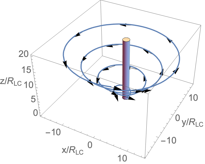
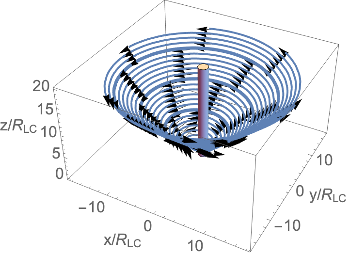
Figure 19: Field lines for Michel’s solution.

Total velocity (differentiating (A2) with respect to time)

$${\bf v}=\beta_{r}{\bf e}_{r}+\sin\theta r\Omega(1-\beta_{r})e_{\phi}$$ (A3)

The Lagrangian then becomes

$${\cal L}=-\sqrt{1-\beta_{r}^{2}-\sin^{2}\theta r^{2}\Omega^{2}(1-\beta_{r})^{2}}$$ (A4)

($\theta=\pi/2$ is assumed below for simplicity).

Lagrange equation for coordinate $r$ with $\beta_{r}=\partial_{t}r$

$$\partial_{r}{\cal L}=\partial_{t}(\partial_{\beta_{r}}{\cal L})$$ (A5)

gives

$$\partial_{t}\beta_{r}=r\Omega^{2}(1-\beta_{r})^{2}(1-r^{2}\Omega^{2}+\beta_{r}(2+r^{2}\Omega^{2}))$$ (A6)

Solution satisfying $r(t=0)=1/\Omega$ is

$$t=r-\frac{1}{\Omega}+\frac{\log\left(\frac{\left(\gamma_{0}^{2}-1\right)(r\Omega-1)\left(\sqrt{\gamma_{0}^{2}+r^{2}\Omega^{2}-1}+\gamma_{0}r\Omega\right)}{\gamma_{0}^{2}(r\Omega+1)\left(\gamma_{0}r\Omega-\sqrt{\gamma_{0}^{2}+r^{2}\Omega^{2}-1}\right)}\right)}{2\Omega}$$ (A7)

where the integration constant $\gamma_{0}$ was chosen to match (17). Differentiating (A7) with respect to time we recover (17).

As a check, let us repeat the above derivation using Hamiltonian approach. Given Lagrangian (A4) we can find canonical momentum $P_{r}$ and Hamiltonian

$$P_{r}=\partial_{\beta_{r}}{\cal L}=\frac{\beta_{r}-r^{2}\Omega^{2}\left(1-\beta_{r}\right)}{\sqrt{1-\beta_{r}^{2}-r^{2}\Omega^{2}(1-\beta_{r})^{2}}}\mbox{}$$

$${\cal H}={\beta_{r}}P_{r}-{\cal L}=\frac{r^{2}\Omega^{2}P_{r}+\sqrt{P_{r}^{2}+r^{2}\Omega^{2}+1}}{r^{2}\Omega^{2}+1}\mbox{}$$

Canonical equations are then

$$\beta_{r}=\partial_{t}r=\partial_{P_{r}}{\cal H}=\frac{r^{2}\Omega^{2}}{1+r^{2}\Omega^{2}}+\frac{P_{r}}{(1+r^{2}\Omega^{2})\sqrt{1+P_{r}^{2}+(r\Omega)^{2}}}\mbox{}$$

$$\partial_{t}P_{r}=-\partial_{r}{\cal H}=\frac{r\Omega^{2}\left(-2P_{r}\sqrt{P_{r}^{2}+r^{2}\Omega^{2}+1}+2P_{r}^{2}+r^{2}\Omega^{2}+1\right)}{\left(r^{2}\Omega^{2}+1\right)^{2}\sqrt{P_{r}^{2}+r^{2}\Omega^{2}+1}}$$ (A9)

Equating ${\cal H}=\gamma_{0}$ we find

$$P_{r}=\frac{\gamma_{0}r^{2}\Omega^{2}+\sqrt{\gamma_{0}^{2}+r^{2}\Omega^{2}-1}}{1-r^{2}\Omega^{2}}$$ (A10)

Using (A10) in expression for velocity (A9) we recover (17).

The Lagrangian approach requires integration of the equations of motion and allows one to find $r(t)$, while the more simple Hamilton-Jacobi approach, which involves only algebraic relations, gives only $\beta_{r}(r)$. This is sufficient for our application.

Appendix B Another Lagrangian approach in Schwarzschild metric

Let us next extend the results of Appendix A to Schwarzschild metric using a somewhat different approach. We are interested in getting the radial speed of the particle along the string (i.e., on the (1+1)-D manifold). The alternative choice of Lagrangian is

$$\mathcal{L}(\dot{t},\dot{r},r)=\frac{1}{2}\left[-G_{00}\,\dot{t}^{2}+G_{rr}\,\dot{r}^{2}+2G_{0r}\,\dot{t}\dot{r}\right],\hskip 56.9055pt\dot{x}=\frac{dx}{d\tau}$$ (B1)

From the symmetry of the Lagrangian in the $t$ coordinate, we use the Euler-Lagrange equation to get

$$\dot{t}=\frac{G_{0r}\,\dot{r}+E}{G_{00}\,},\hskip 56.9055ptG_{00}\,\neq 0$$ (B2)

where $E$ is a constant of motion. It is generally different from $\gamma_{0}$ - different choices of the Lagrangian result in different integration constants; the exact relations between different constants are typically complicated.

Again, using Euler-Lagrange equations for the radial coordinate, we get

$$2\ddot{r}\Gamma(r)+\dot{r}^{2}\frac{d}{dr}\Gamma(r)+E^{2}\frac{d}{dr}\frac{1}{G_{00}\,}=0$$ (B3)

We use the following trick,

$$r=r(\tau)\Rightarrow\ddot{r}=\frac{d\dot{r}}{d\tau}=\dot{r}\frac{d\dot{r}}{dr}=\frac{1}{2}\frac{d}{dr}\dot{r}^{2}\hskip 5.69046pt\Rightarrow\hskip 5.69046pt2\ddot{r}\Gamma(r)+\dot{r}^{2}\frac{d}{dr}\Gamma(r)=\frac{d}{dr}\left(\Gamma(r)\dot{r}^{2}\right)$$ (B4)

Now, the equation of motion becomes

$$\frac{d}{dr}\left(\Gamma(r)\dot{r}^{2}+\frac{E^{2}}{G_{00}\,}\right)=0$$ (B5)

Since all the functions of the radial coordinate in the equation of motion are all positive within the DOC, then we can say that we have a first-order differential equation that is equal to a non-negative constant. In other words, we say

$$\boxed{\Gamma(r)\dot{r}^{2}+\frac{E^{2}}{G_{00}\,}=\alpha^{2}},\hskip 28.45274pt\alpha^{2}=\Gamma(r_{0})\dot{r_{0}}^{2}+\frac{E^{2}}{G_{00}(r_{0})},\hskip 7.11317ptr_{0}:=r(\tau_{0}),\dot{r}_{0}:=\dot{r}(\tau_{0})$$ (B6)

Therefore, we have

$$\boxed{\dot{r}^{2}=\frac{\alpha^{2}G_{00}\,-E^{2}}{G_{00}\,G_{rr}\,+G_{0r}^{2}}}$$ (B7)

We are interested in getting a relationship between the radial and the time coordinates, i.e. $r=r(t)$. To do so, we note that

$$v_{r}=\frac{dr}{dt}=\frac{\dot{r}}{\dot{t}}\Rightarrow G_{00}\,\dot{t}=G_{0r}\,v_{r}\dot{t}+E\iff\dot{t}=\frac{E}{G_{00}\,-G_{0r}\,v_{r}}$$ (B8)

So, we rewrite the equation of velocity as

$$v_{r}(r)=G_{00}\,\left(G_{0r}\,+\sqrt{\frac{G_{00}\,G_{rr}\,+G_{0r}^{2}}{\epsilon^{2}G_{00}\,-1}}\right)^{-1}$$ (B9)

After some calculations, we get

$$\boxed{t=t_{0}+\int_{r_{0}}^{r}\left(\frac{G_{0r}\,}{G_{00}\,}+\frac{1}{G_{00}\,}\sqrt{\frac{G_{00}\,G_{rr}\,+G_{0r}^{2}}{\epsilon^{2}G_{00}\,-1}}\right)dr}\hskip 28.45274pt\epsilon=\frac{\alpha}{E}$$ (B10)

Note that this puts a restriction on the value of $G_{00}\,$, since

$$G_{00}\,>\epsilon^{2},\hskip 28.45274pt\forall r\in\text{DOC}$$ (B11)

Hence, this is also true for $r_{ext}$:

$$G_{00}(r_{ext})>\epsilon^{2}\Rightarrow 0\leq 3m<(1-\epsilon^{2})r_{ext}$$ (B12)

Because the radial coordinate is always non-negative, we conclude that

$$0\leq\epsilon^{2}<1\iff 0\leq\alpha^{2}<E^{2}$$ (B13)

More precisely, we get the following constraint on both constants of motion, $\alpha$ and $E$,

$$0\leq\epsilon^{2}<1-(9m^{2}\Lambda^{\prime})^{\frac{1}{3}}\leq 1\iff\boxed{0\leq\epsilon^{2}<1-(3m^{2}(\Lambda+3\Omega^{2}))^{\frac{1}{3}}\leq 1}$$ (B14)

One last thing, there is a point in the DOC where the gravitational attraction of the black hole equals to the repulsive force of rotation. At that point, the velocity is zero. In other words,

$$\epsilon^{2}G_{00}\,=1$$ (B15)

We have done some analysis for our general problem. Let us consider the physics, i.e. we consider the physical situations by setting a specific function of $r$ for the new angle coordinate, $\phi(r)$.

Let us solve it in another way. We start from

$$\mathcal{L}(\dot{r},r)=\Gamma(r)\dot{r}^{2}-\frac{E^{2}}{G_{00}\,}$$

For timelike trajectories,

$$\mathcal{L}(\dot{r},r)=\frac{1}{2}\left[\left(G_{rr}\,+\frac{G_{0r}^{2}}{G_{00}}\right)\dot{r}^{2}-\frac{E^{2}}{G_{00}\,}\right]=-\frac{1}{2}$$ (B16)

The speed of the coordinate $r$ with respect to the proper time (the time measured by the particle that is constrained to move along the string) is

$$\dot{r}=\pm\sqrt{\frac{E^{2}-G_{00}\,}{G_{0r}^{2}+G_{00}\,G_{rr}\,}}$$ (B17)

The sign here determines the direction of motion: either towards or away from the black hole. The speed of the coordinate $r$ with respect to the coordinate $t$ is

$$\beta_{r}=\frac{dr}{dt}=\frac{\dot{r}}{\dot{t}}\>\overset{(\ref{tDOT})}{=}\>G_{00}\,\left(G_{0r}\,+\frac{E}{\dot{r}}\right)^{-1}=G_{00}\,\left(G_{0r}\,\pm E\sqrt{\frac{G_{0r}^{2}+G_{00}\,G_{rr}\,}{E^{2}-G_{00}\,}}\right)^{-1}$$ (B18)

This recovers equation (14), obtained by the Hamilton-Jacobi approach.

The trajectory is

$$t=t_{0}+\int_{r_{0}}^{r}\frac{1}{G_{00}(r^{\prime})}\left[G_{0r}(r^{\prime})\pm E\sqrt{\frac{G_{0r}^{2}(r^{\prime})+G_{00}(r^{\prime})G_{rr}(r^{\prime})}{E^{2}-G_{00}(r^{\prime})}}\right]dr^{\prime}$$ (B19)

Consider rotating magnetosphere in Schwarzschild metric. We use the following convention

$$G_{00}=\alpha^{2}-r^{2}\Omega^{2},\hskip 14.22636ptG_{rr}=\frac{1}{\alpha^{2}}+\frac{r^{2}\Omega^{2}}{\alpha^{4}},\hskip 14.22636ptG_{0r}=-\frac{r^{2}\Omega^{2}}{\alpha^{2}}$$ (B20)

The Lagrangian is then

$${\cal L}=\frac{1}{2}\left(-\alpha^{2}\left(1-\frac{r^{2}\Omega^{2}}{\alpha^{2}}\right)\,\dot{t}^{2}+\frac{1}{\alpha^{2}}\left(1+\frac{r^{2}\Omega^{2}}{\alpha^{2}}\right)\,\dot{r}^{2}-2\frac{r^{2}\Omega^{2}}{\alpha^{2}}\,\dot{t}\dot{r}\right)$$ (B21)

Between the two light cylinders, the constant of motion

$$E=\left(\alpha^{2}-r^{2}\Omega^{2}\right)\dot{t}+\frac{r^{2}\Omega^{2}}{\alpha^{2}}\dot{r}$$ (B22)

We then get $\dot{r}$ by substituting in (B17) or by solving the quadratic equation (B21) using $G_{00}G_{rr}+G_{0r}^{2}=1$ (in our case):

$$\dot{r}=\frac{-G_{0r}\dot{t}\pm\sqrt{\dot{t}^{2}-G_{rr}}}{G_{rr}}$$ (B23)

Eliminating $\dot{t}$ with (B22),

$$\dot{t}=\frac{\alpha^{2}E-r^{2}\Omega^{2}\dot{r}}{\alpha^{2}\left(\alpha^{2}-r^{2}\Omega^{2}\right)}$$ (B24)

we find Lagrangian and Hamiltonian

$${\cal L}=\frac{\dot{r}^{2}-E^{2}}{2\left(\alpha^{2}-r^{2}\Omega^{2}\right)}\mbox{}$$

$${\cal H}=\dot{r}\partial_{\dot{r}}{\cal L}-{\cal L}=\frac{\dot{r}^{2}+E^{2}}{2\left(\alpha^{2}-r^{2}\Omega^{2}\right)}$$ (B25)

Finally, we obtain

$$(\dot{r}+\gamma_{0}G_{0r})^{2}=(G_{0r}\dot{r}+\gamma_{0})^{2}-G_{00}^{2}G_{rr}\hskip 14.22636pt\xrightarrow{G_{00}G_{rr}+G_{0r}^{2}=1}\hskip 14.22636pt\dot{r}^{2}=\frac{G_{00}G_{rr}(\gamma_{0}^{2}-G_{00})}{1-G_{0r}^{2}}=\gamma_{0}^{2}-G_{00}$$ (B26)

We used ($\sqrt{2}$ times) the proper time to parameterize the Lagrangian in (B21); thus, the Lagrangian has a constant value of $-1/2$ with this parameterization for timelike geodesics. Therefore, $\dot{r}$ is

$$\dot{r}=\pm\sqrt{r^{2}\Omega^{2}+E^{2}-\alpha^{2}},$$ (B27)

consistent with (26).

COMMENT: I COULD NOT WORK WITH THE HAMILTONIAN; I GET TAUTOLOGY($\dot{r}=\dot{r}$) SO, I COMMENTED THE HAMILTONIAN PART AND GOT $\dot{r}$ IN A DIFFERENT, BUT EQUIVALENT WAY Alternatively, we can get $\dot{r}$ from the

$${\cal L}(\dot{r},r)=\frac{\dot{r}^{2}-\gamma_{0}^{2}}{2\left(\alpha^{2}-r^{2}\Omega^{2}\right)}=-\frac{1}{2}\rightarrow\dot{r}^{2}=-\alpha^{2}+\gamma_{0}^{2}+r^{2}\Omega^{2}$$ (B28)

The radial velocity measured by the coordinate time of the observer is then

$$\beta_{r}=\frac{\dot{r}}{\dot{t}}=\frac{\alpha^{2}\left(\alpha^{2}-r^{2}\Omega^{2}\right)}{\frac{\alpha^{2}E}{\sqrt{r^{2}\Omega^{2}+E^{2}-\alpha^{2}}}-r^{2}\Omega^{2}}$$ (B29)

The geodesic equation takes a nice form

$$\ddot{r}=\frac{1}{2}\frac{d}{dr}\left(\dot{r}^{2}\right)=r\Omega^{2}-\frac{M}{r^{2}},$$ (B30)

(derivatives are with respect to proper time) which unites the cases of radial motion in Schwarzschild geometry (e.g. Misner et al., 1973) and (26).

We also note that one can get the same differential equation (for the case between the two light cylinders) by solving the classical mechanical problem of a particle with mass $m$ constrained to move along a straight wire rotating with a constant angular speed $\Omega$ in the flat 2-D plane, with the inclusion of a source of mass $M$ at the center. The Lagrangian is ($\dot{r}=dr/dt$)

$$\mathcal{L}=\frac{1}{2}m\left(\dot{r}^{2}+r^{2}\Omega^{2}\right)-U(r),\hskip 28.45274ptU(r)=-m\frac{MG}{r}$$ (B31)

Appendix C

This relation can also be derived from

$${\cal H}=-P_{0}=\frac{G^{0r}P_{r}}{G^{00}}+\sqrt{\frac{G^{rr}G_{r}^{2}+1}{-G^{00}}+\left(\frac{G^{0r}P_{r}}{G^{00}}\right)^{2}}$$ (C1)

On the other hand

$${\cal L}=\frac{1}{2}G_{\mu\nu}u^{\mu}u^{\nu}=\frac{1}{2}(u_{0}-u_{r})((u_{0}+u_{r})r^{2}\Omega^{2}+u_{r}-u_{0})\hskip 14.22636pt\left[\frac{1}{2}(u_{0}+u_{r})((u_{0}+u_{r})r^{2}\Omega^{2}+u_{r}-u_{0})\right]$$ (C2)

In passing we comment on a bead-on-straight-wire problem. In that case the coordinate acceleration is

$$\partial_{t}\beta_{r}=r\Omega^{2}\left(1-\frac{2\beta_{r}^{2}}{1-r^{2}\Omega^{2}}\right)$$ (C3)

The reversal of the sign on the coordinate acceleration in this case is a purely coordinate effect, not physical, effect (2009arXiv0903.1113L). Similar “reversal” appears for when radial step of the spiral is large, $\Omega_{1}<\Omega$, see §3.5.

Appendix D Limitations on angular velocity of field lines

Transformation to the rotating Kerr metric has limitations (Lyutikov, 2009): it is physical only for angular velocities smaller than $\omega_{ph}$, angular velocity of a photon orbit, defined by the conditions of circular rotation with the speed of light $g_{00}=0,\,\partial_{r}g_{00}=0$. This gives $-4a^{2}M+r(-3M+r)^{2}=0$ (Bardeen et al., 1972). For a given $a$ and $r$, the transformation to the rotating Kerr metric becomes meaningless for $\omega$ higher than the angular velocity of a photon circular orbit,

$$\omega_{\rm ph}={1\over\mp|a|+6M\cos({1\over 3}{\rm arccos}(\mp|a|/M)}$$ (D1)

The upper sign corresponds to prograde rotation. Particular values are $a=0,\,r_{\rm ph}=3M,\,\omega_{\rm ph}=1/(3\sqrt{3}M)$ for Schwarzschild black hole, $a=M,\,r_{\rm ph}=M,\,\omega_{\rm ph}=1/(2M)$ for prograde and $a=-M,\,r_{\rm ph}=4M,\,\omega_{\rm ph}=1/(7M)$ for retrograde photon orbits. For $1/(7M)<\omega<1/(2M)$ this requires sufficiently high $a$, satisfying $\omega<1/\left(a+2\sqrt{2}M\left(1+\cos\left({2\over 3}{\rm arccos}(-{a\over M})\right)\right)\right)^{3/2}$ (for $a=0$ this requires $\omega<1/(3\sqrt{3})$). For $\omega\rightarrow 1/(2M)$ both light cylinders merge on the black hole horizon at $a=M=r$. For higher $\omega$, the transformation to the rotating frame becomes meaningless everywhere (Fig. 20).

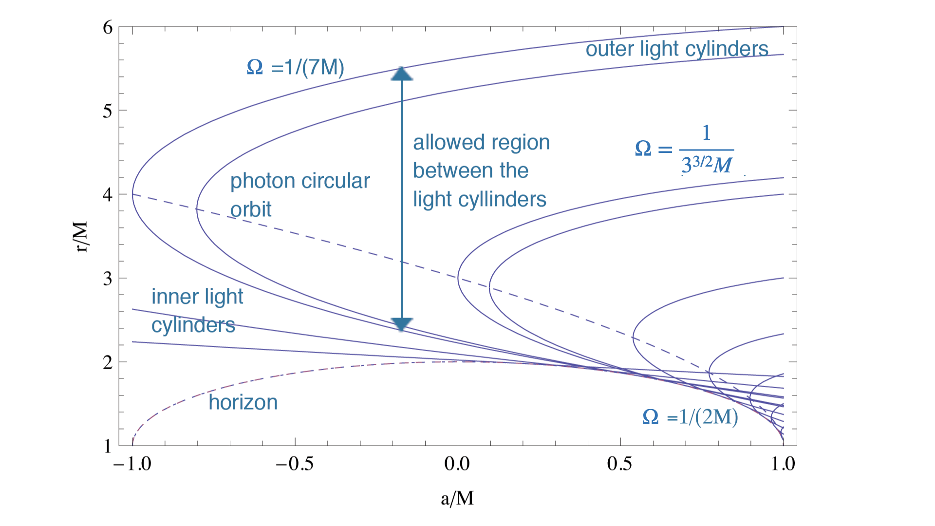
Figure 20: The locations of light cylinders for different $\omega$ as function of $a$. The light cylinders always lie outside the horizon (dotted curve). For a given $\omega$, the inner and outer light cylinders merge at the photon circular orbit (dashed line). The physically meaningful region lies in between the light cylinders, to the right of the light cylinders curve. For $\omega\rightarrow 0$, the inner light cylinder  coincides with the ergosphere $r=2M$. As $\omega$ increases, the outer light cylinder moves to smaller $r$; the radial location of the inner light cylinder  is a complicated function of $\omega$. For $\omega>1/(7M)$ there is a region for sufficiently small $a$, for which the transformation to the rotating frame is unphysical. For high $\omega\rightarrow 1/(2M)$ and high $a>M/\sqrt{2}$, the inner light cylinder moves inside the ergosphere of a Kerr black hole. For $\omega>1/(2M)$, the transformation to rotating frame is unphysical everywhere. Adapted from (Lyutikov, 2009)

D.1 The Invariant Radial Speed Constraints

COMMENT: I SUGGEST REMOVING THIS SUBSECTION, IT HAS INFO BUT I DO NOT KNOW IF IT IS IMPORTANT We obtained the set of values that the time constant $E$ only take; consequently, from (E72), we can obtain the set of allowed values to the (initial) radial speed as observed by the fixed observers along the string. Furthermore, as a check for the result (E86), we are going to show that this initial speed vanishes and remains zero only if the particle is at the null line. From (E90), (E72), and (E73), we get

$$1-\frac{1-a^{2}\eta^{2}-3\eta^{\frac{2}{3}}(1-a\eta)^{\frac{4}{3}}}{G_{00}}\leq v^{2}(r)<1-\frac{1-a^{2}\eta^{2}}{G_{00}}$$ (D2)

$$1-\frac{1-a^{2}\eta^{2}-3\eta^{\frac{2}{3}}(1-a\eta)^{\frac{4}{3}}}{G_{00}(r_{0})}\leq v_{0}^{2}<1-\frac{1-a^{2}\eta^{2}}{G_{00}(r_{0})}$$ (D3)

A zero invariant radial speed is equivalent to the equality case of the inequality (E87)

$$G_{00}=E^{2}\iff\Omega^{2}r^{3}-(1-a^{2}\eta^{2}-E^{2})r+2M(1-a\eta)^{2}=0\hskip 28.45274ptr\in(r_{1},r_{2})$$ (D4)

IS THIS CORRECT?? $v(R_{0})=0\>but\>v_{0}(r_{0})>0\>and\>r_{0}>R_{0}$

This cubic equation is always non-negative from (E87). Nevertheless, we focus now on the special case that it is zero. Therefore, we just modify the constraints in (E89) to be

$$\Omega^{\,2}r^{3}-br+\frac{1}{3\sqrt{3}}\>\frac{2b^{\frac{3}{2}}}{\Omega}=0,\hskip 56.9055ptb>0$$ (D5)

Thus, the only case that this equation is zero is when its minimum is zero. From (E7), the minimum radius is

$$r_{min}=\sqrt{\frac{b}{3\Omega^{2}}}=\sqrt{\frac{1-a^{2}\eta^{2}-E^{2}}{3\Omega^{2}}}\hskip 28.45274pt\xrightarrow[(\ref{NullLine})]{(\ref{AllConstraints})}\hskip 28.45274ptr_{min}\in(0,R_{0}]$$ (D6)

Since the fixed observers along the string are only defined between the two light cylinders as well as the null line, the invariant radial speed is also defined in the same domain. Therefore, we are restricted to only work with the cases where $r_{min}$ is defined between the two light cylinders.

$$v(r_{min})=0\hskip 85.35826ptr_{min}\in(r_{1},R_{0}]$$ (D7)

IGNORE THIS TEXT Let us apply some initial conditions. We place a particle on the null line with the initial Lorentz factor $\gamma_{0}$ along the 1-D path it will follow. Let us calculate the Energy from (LABEL:EnergyConstraintsInGeneral). If we start with zero initial radial speed, we get

$$E=\frac{G_{00}(r_{0})}{\sqrt{A_{1}(r_{0})}-\frac{\Omega G_{1}(r_{0})}{A_{1}(r_{0})}}=\frac{E^{2}}{\sqrt{A_{1}(r_{0})}-\frac{\Omega G_{1}(r_{0})}{A_{1}(r_{0})}}$$ (D8)

THEN WHAT??? This result does not make any sense because $v_{0}$ must be zero always! What is the meaning of having non-zero radial speed everywhere if we start with such initial conditions???

These fixed observers are not fixed relative to the (2+1)-D manifold of an observer with the Kerr metric. So, we have to find out a way to solve this. Here is a suggestion

The fixed observers are also rotating observers (from the prospective of the (2+1)-D Kerr observers) according to the equation

$$\dot{\phi}=\frac{d\phi}{d\tau}=\frac{d\phi/dt}{d\tau/dt}=\Omega\dot{t}$$ (D9)

And they have a four-velocity vector of

$$U^{\mu}_{rot}=\dot{t}\begin{pmatrix}1\\ 0\\ \Omega\end{pmatrix}\xrightarrow[\mathcal{L}=-1,\>\dot{\phi}=\Omega\dot{t}]{\mathcal{L}=g_{00}\,\dot{t}^{2}+g_{\phi\phi}\,\dot{\phi}^{2}+2g_{0\phi}\,\dot{t}\dot{\phi}}U^{\mu}_{rot}=\frac{1}{\sqrt{G_{00}\,}}\begin{pmatrix}1\\ 0\\ \Omega\end{pmatrix}$$ (D10)

These rotating observers see a particle that moves with

$$\gamma_{1}(r)=\gamma(r_{0})\sqrt{\frac{G_{00}(r_{0})}{G_{00}\,}}$$ (D11)

Let us get the relative Lorentz factor of the rotating observers as seen by fixed observers (both in the Kerr metric). For the fixed observers,

$$U_{\mu}^{fixed}=\begin{pmatrix}g_{00}\,&&0&&g_{0\phi}\,\end{pmatrix}$$ (D12)

The fixed observers see the rotating ones (both in the Kerr metric) move with a relative Lorentz factor of

$$\gamma_{2}(r)=-U_{\mu}^{fixed}U^{\mu}_{rot}=\frac{-g_{00}\,-\Omega g_{0\phi}\,}{G_{00}\,}$$ (D13)

We calculate the following when the particle, the rotating observers of the Kerr, and the fixed observers of the Kerr all are at the same point of spacetime. We can get the relative Lorentz factor of the particle as seen by the fixed observers of the Kerr.

I DO NOT THINK THAT THIS IS IMPORTANT Note that

$$v(r_{0})\geq 1\Rightarrow v(r)\geq 1$$ (D14)

SUBTLETY IS HERE: Why do we have a required initial minimum speed?

In case the initial speed is less than unity (the speed of light), we note that the second term is negative, with a minimum negative value occurs when the initial speed is zero. At this point, we have the following constraint (or otherwise the observed velocity will be imaginary)

$$G_{00}\,\leq G_{00}(r_{0})$$ (D15)

We know that at the null point $r_{0}=\eta^{-\frac{2}{3}}$, this condition is always satisfied. So,

Rewriting (LABEL:ObservedVelocityCompleted) in a more standard form

$$\gamma(r)=\gamma_{0}\sqrt{\frac{G_{00}(r_{0})}{G_{00}\,}}$$ (D16)

In the specific case of the metric we have been using, while starting from the null point, we get

$$\gamma(r)=\gamma_{0}\sqrt{\frac{G_{00}(r_{0})}{G_{00}\,}}\hskip 56.9055ptr_{0}=\eta^{-\frac{2}{3}}$$ (D17)

We will set the boundaries we have on the time constant in terms of the spacetime parameters (and others) and get back to this equation to talk about the boundaries on the initial Lorentz factor, if there is any (of course we should get $v(r_{0})<1$ is a must).

DO WE NEED THIS?

Back to equation (LABEL:ObservedVelocityCompleted), we have a constraint on the initial speed as follows: we are sure that it does not exceed the speed of light because $G_{00}(r_{0})>0$; so, it has a minimum of zero that does not attain. Then, we have

$$G_{00}(r_{0})<0\Rightarrow 1+3\eta^{\frac{2}{3}}G_{00}(r_{0})<1$$ (D18)

Moreover, we have an upper bound to that function

$$G_{00}\,\leq 1-3\eta^{\frac{2}{3}}\iff 3\eta^{\frac{2}{3}}\leq 1+G_{00}\,$$ (D19)

Thus,

$$\left\{\begin{array}[]{cc}3\eta^{\frac{2}{3}}\leq 1+G_{00}(r_{0})\leq v^{2}(r_{0})\leq 1-3\eta^{\frac{2}{3}}G_{00}(r_{0})<1,\hskip 14.22636pt\eta<\frac{1}{3\sqrt{3}}&:\eta\neq 0\\ 0\leq 1+G_{00}(r_{0})\leq v^{2}(r_{0})<1&:\eta=0\end{array}\right.$$ (D20)

Generally speaking,

$$\boxed{3\eta^{\frac{2}{3}}\leq v^{2}(r_{0})<1}$$ (D21)

If the initial invariant radial speed at the null line (E86) is zero, the final one there is zero too. From (E72),

$$v_{0}(R_{0})=0\iff E^{2}=G_{00}(R_{0})=1-a^{2}\eta^{2}-3\eta^{\frac{2}{3}}(1-a\eta)^{\frac{4}{3}}\mbox{}$$

$$v(r)=0\iff G_{00}(r)=E^{2}=G_{00}(R_{0})$$ (D22)

Then, we conclude that $r=R_{0}$: the particle remains at the null line.

Appendix E Kerr Black Hole Analysis

In this Appendix, we calculate the velocity components relative to an observer at infinity and show that the radial component dominates in a few light cylinder radii; we also obtain the Lorentz factor of the speed relative to both fixed observers in spacetime and co-rotating observers with the field lines.

We consider a (2+1)-D manifold of the Kerr black hole with a constant $\theta$. Then, we move to a (1+1)-D sub-manifold that is rotating with a constant angular speed $\Omega$ according to

$$d\phi=\Phi^{\prime}(r)\,dr+\Omega\,dt\hskip 56.9055pt\Phi^{\prime}(r)=\frac{d\Phi(r)}{dr}$$ (E1)

This means that a particle in this sub-manifold is constrained to move along a wire with a shape function $\Phi(r)$. Using the formula in (5), we define the wire function as follows:

$${\Phi^{\prime}(r)=\omega_{sp}=-\sqrt{\frac{g_{rr}}{g_{00}}}\left(\frac{g_{0\phi}}{g_{\phi\phi}}+\Omega_{1}(r)\right)}$$ (E2)

where $\Omega(r)$ is a function of the radial coordinate as a generalization of the Archimedean spiral shape (e.g., $\Omega_{1}(r)=\Omega$ is the Archimedean spiral case). We note from (38) that this function has some constraints to have a physically realizable spiral step (like in the Schwarzshild metric, $\Omega_{1}(r)\geq\Omega$). Using the notation in (7), the metric of is

$$ds^{2}=-G_{00}\,dt^{2}+G_{rr}\,dr^{2}+2G_{0r}\,dtdr\mbox{}$$

$$G_{00}\,=g_{00}\,-(\Omega g_{\phi\phi}\,+2g_{0\phi}\,)\Omega\mbox{}$$

$$G_{rr}\,=g_{rr}\,+\Phi^{\prime}(r)^{\,2}\,g_{\phi\phi}\,\mbox{}$$

$$G_{0r}\,=\left(\Omega g_{\phi\phi}\,+g_{0\phi}\,\right)\Phi^{\prime}(r)$$ (E3)

The condition for finding the horizons (here, the light cylinders) is

$$G^{\,rr}=0\hskip 14.22636pt\xrightarrow[]{G\neq 0}\hskip 14.22636ptG_{00}\,=0$$ (E4)

From the definition of $G_{00}$ in (E), we see that the location of the light cylinders is independent of the shape of the wire $\Phi(r)$. The current spacetime is a conic one, with a subtended angle of $\theta$. We go to the equatorial plane ($\theta=\pi/2$); so, we get the light cylinders by solving

$$-\Omega^{2}r^{3}+(1-a^{2}\eta^{2})r-2M(1-a\eta)^{2}=0,\hskip 56.9055pt\eta=M\Omega$$ (E5)

With regarding the dimensions, note that both $\eta$ and the black hole spin parameter $a$ are dimensionless quantities. Let us get some insights about the general cubic equation:

$$\Omega^{\,2}r^{3}-br+d=0,\hskip 56.9055ptd\geq 0$$ (E6)

In order to get the roots, the local minimum (maximum) of such a function of $r$ has to be at most (least) zero. Hence, we have some constraints on the constants

$$r_{ext}=\frac{1}{\Omega}\sqrt{\frac{b}{3}}\hskip 14.22636pt\xrightarrow[]{r_{ext}>0}\hskip 14.22636ptb>0\hskip 14.22636pt\Rightarrow\hskip 14.22636ptd>0$$ (E7)

since $b$ and $d$ are related to one another in (E5). The extreme point is indeed a local minimum point:

$$\frac{d^{2}}{dr^{2}}\left(\Omega^{\,2}r^{3}-br+d\right)_{r_{ext}}=6\,\Omega^{\,2}\,r_{ext}>0$$ (E8)

For finding the roots, we demand that the cubic equation at the minimum radius to be negative (we need to allow for more than one light cylinder to have a non-empty working domain, as we are going to explain later)

$$\Omega^{\,2}r_{ext}^{3}-br_{ext}+d\leq 0\hskip 14.22636pt\Rightarrow\hskip 14.22636ptd<\frac{1}{3\sqrt{3}}\>\frac{2b^{\frac{3}{2}}}{\Omega}$$ (E9)

Then, we have constraints on $b$ and $d$, and the equation becomes

$$\Omega^{\,2}r^{3}-br+d=0,\hskip 56.9055ptb>0,\>0<d<\frac{1}{3\sqrt{3}}\>\frac{2b^{\frac{3}{2}}}{\Omega}$$ (E10)

We conclude the following constraint in our problem

$$\eta\sqrt{\frac{(1-a\eta)}{(1+a\eta)^{3}}}<\frac{1}{3\sqrt{3}}\hskip 28.45274pt\xrightarrow[]{a=0}\hskip 28.45274pt\eta<\frac{1}{3\sqrt{3}}$$ (E11)

which reduces to the known constraint if the black hole is not rotating. Figure (20) plots this inequality for specific cases of the mass-rotation parameter $\eta$.

Using the constraints (E19), we find that there are two real solutions to equation (E5). In other words, there are two light cylinders: the inner light cylinder (with radius $r_{1}$), and the outer light cylinder (with radius $r_{2}>r_{1}$). Notice that $G_{00}\,$ is always positive in the region between the two light cylinders.

In order to know the valid boundaries of the problem inside the rotating FR, we must examine the signature of the metric (LABEL:SchArchMetric). We diagonalized the metric tensor (using Mathematica), and found that the sign of the function $\phi^{\prime}(r)$ does not really matter in determining the metric signature (because the eigenvalues are only functions of $\phi^{\prime}(r)^{2}$). Thus, to determine the location of the DOC, where the light cylinders are and causality still holds, we just have to consider the diagonal functions of the metric (LABEL:SchArchMetric). Therefore, this is sort of the same as what had been done with the Schwarzschild metric; the signature is only determined by the first two diagonal terms, i.e., the functions in front of $dt^{2}$ and $dr^{2}$.

We see that the term in front of $dr^{2}$ of (LABEL:SchArchMetric) is always positive while being within DOC. So, let us check the first term of the same metric. We want to preserve the metric signature of $(-,+,+,+)$, so, we demand

$$G_{00}\,=f(r)-r^{2}\Omega^{2}>0\iff 1-\frac{2m}{r}-\Omega^{2}r^{2}>0$$ (E12)

We can argue that if we increase the angular speed, the two light cylinders go closer to each other until they meet.

1. The range of the radius coordinate is

   $$G_{00}\,<0\iff r\left(\Omega^{2}r^{2}-(1-a^{2}\eta^{2})\right)<-2M(1-a\eta)^{2}<0\hskip 5.69046pt\Rightarrow\hskip 5.69046ptr<\frac{\sqrt{1-a^{2}\eta^{2}}}{|\Omega|}\mbox{}$$

   $$G_{00}\,<0\iff(1-a^{2}\eta^{2})r-2M(1-a\eta)^{2}>\Omega^{2}r^{3}>0\hskip 5.69046pt\Rightarrow\hskip 5.69046ptr>2M\frac{1-a\eta}{1+a\eta}\mbox{}$$

   $$\boxed{2M\frac{1-a\eta}{1+a\eta}<r<\frac{\sqrt{1-a^{2}\eta^{2}}}{|\Omega|}}$$ (E14)

2. The two light cylinders meeting point is

3. From (LABEL:SchArchConclusion1), we see that the radius of this light cylinder is greater than one for the black hole event horizon.

4. $$\frac{d}{dr}G_{00}(r_{ext})=0\iff r_{ext}=\left(\frac{m}{\Omega^{2}}\right)^{\frac{1}{3}}$$ (E15)

5. $$\frac{d^{2}}{dr^{2}}G_{00}(r_{ext})=-\frac{4m}{r_{ext}^{3}}-2\Omega^{2}=-6\Omega^{2}<0$$ (E16)

   So, the function $G_{00}\,$ has a maximum at the radius $r_{ext}$.

6. when the extreme value of $G_{00}\,$ is just zero.

   $$G_{00}(r_{ext})=0\iff r_{ext}=3M\frac{1-a\eta}{1+a\eta}\hskip 28.45274pt\left(\iff\eta\sqrt{\frac{(1-a\eta)}{(1+a\eta)^{3}}}=\frac{1}{3\sqrt{3}}\right)$$ (E17)

We can see that the two light cylinders exist at radii in the following intervals

$$2M\frac{1-a\eta}{1+a\eta}<r_{1}<3M\frac{1-a\eta}{1+a\eta}\hskip 56.9055pt3M\frac{1-a\eta}{1+a\eta}<r_{2}<\frac{\sqrt{1-a^{2}\eta^{2}}}{|\Omega|}$$ (E18)

Moreover, while increasing the value of the angular speed, the light cylinder that is close to (far from) the black hole moves outwards (towards) the black hole horizon, respectively; they eventually meet at the radius in (E17).

Note that we have constraints on the values of the mass-rotation parameter $\eta=M\Omega$ and the Kerr parameter $a$:

$$\eta\sqrt{\frac{(1-a\eta)}{(1+a\eta)^{3}}}<\frac{1}{3\sqrt{3}}$$ (E19)

In the Kerr case, we have (by definition) the following coordinate basis vectors

$$(\boldsymbol{e}_{0})^{\mu}=\left(\begin{array}[]{cc}1\\ 0\\ 0\end{array}\right)\hskip 56.9055pt(\boldsymbol{e}_{r})^{\mu}=\left(\begin{array}[]{cc}0\\ 1\\ 0\end{array}\right)\hskip 56.9055pt(\boldsymbol{e}_{\phi})^{\mu}=\left(\begin{array}[]{cc}0\\ 0\\ 1\end{array}\right)$$ (E20)

Of course, these basis vectors satisfy $\boldsymbol{e}_{\mu}\cdot\boldsymbol{e}_{\nu}=g_{\mu\nu}$. The lengths are

$$|\boldsymbol{e}_{\mu}|=\sqrt{g_{\mu\mu}}\hskip 28.45274pt\Rightarrow\hskip 28.45274pt|\boldsymbol{e}_{0}|=\sqrt{-g_{00}}\hskip 28.45274pt|\boldsymbol{e}_{r}|=\sqrt{g_{rr}}\hskip 28.45274pt|\boldsymbol{e}_{\phi}|=\sqrt{g_{\phi\phi}}$$ (E21)

To get the velocity components, we need to take the total (intrinsic) derivative of the normalized position vector components $\hat{V}^{\mu}$ (note $v^{\mu}:=dx^{\mu}/dt$)

$$\frac{D}{Dt}\hat{V}^{\mu}=|\boldsymbol{e}{{}_{\mu}}{}|\left[\frac{d}{dt}\left(\frac{\hat{V}^{\mu}}{|\boldsymbol{e}{{}_{\mu}}{}|}\right)+\left(\Gamma^{\mu}_{\alpha\beta}v^{\beta}\right)\left(\frac{\hat{V}^{\alpha}}{|\boldsymbol{e}{{}_{\alpha}}{}|}\right)\right]$$ (E22)

We obtain the velocity components as follows

1. The radial component $\beta_{r}$

   $$\beta_{r}=\frac{D}{Dt}\hat{V}^{r}=\frac{D}{Dt}r=v^{r}\left(1+r\left(\frac{1}{2}\frac{d}{dr}\ln(g_{rr})-\frac{1}{2}\frac{d}{dr}\ln(g_{rr})\right)\right)=v^{r}$$ (E23)

   Thus, we are right about our calculations that

   $$\beta_{r}=\frac{Dr}{Dt}=\frac{dr}{dt}$$ (E24)

2. The azimuthal component

   $$\beta_{\phi}=\frac{D}{Dt}\hat{V}^{\phi}=\frac{\sqrt{g_{rr}g_{\phi\phi}}}{2r\sin^{2}{\theta}}\left[g_{00}^{2}\frac{d}{dr}\left(\frac{g_{0\phi}}{g_{00}}\right)+\left[\beta_{r}\Phi^{\prime}(r)+\Omega\right]\left(g_{00}\frac{dg_{\phi\phi}}{dr}+g_{0\phi}\frac{dg_{0\phi}}{dr}\right)\right]$$ (E25)

The velocity vector can be written as (still working in the normalized basis)

$$\boldsymbol{v}=\beta_{r}\hat{\boldsymbol{e}}_{r}+\beta_{\phi}\hat{\boldsymbol{e}}_{\phi}$$ (E26)

In the case of the Schwarzshild metric ($a=0$),

$$\Phi^{\prime}(r)=-\frac{\Omega_{1}(r)}{\alpha^{2}}$$ (E27)

The velocity vector is (see how it reduces to the flat spacetime case in (A3) when we have Archimedean spiral, $\Omega_{1}(r)=\Omega$)

$${\boldsymbol{v}=\beta_{r}\boldsymbol{e}_{r}+r\Omega\left(\alpha-\frac{1}{\alpha}\frac{\Omega_{1}(r)}{\Omega}\beta_{r}\right)\boldsymbol{e}_{\phi}}\hskip 28.45274pt\underset{\alpha=1}{\overset{M=0}{\to}}\hskip 28.45274pt\boldsymbol{v}=\beta_{r}\boldsymbol{e}_{r}+r\Omega\left(1-\frac{\Omega_{1}(r)}{\Omega}\beta_{r}\right)\boldsymbol{e}_{\phi}$$ (E28)

Let us calculate the ratio generally in figure (6) in the equatorial plane

$$\tan(\chi)=\frac{\beta_{\phi}}{\beta_{r}}=\frac{\sqrt{g_{rr}g_{\phi\phi}}}{2r}\left[\frac{g_{00}^{2}}{\beta_{r}}\frac{d}{dr}\left(\frac{g_{0\phi}}{g_{00}}\right)+\left[\Phi^{\prime}(r)+\frac{\Omega}{\beta_{r}}\right]\left(g_{00}\frac{dg_{\phi\phi}}{dr}+g_{0\phi}\frac{dg_{0\phi}}{dr}\right)\right]$$ (E29)

Defining a decreasing (dimensionless) function $\delta(r)$ that is the change between the actual shape of the wire and the approximate form (the Archimedean spiral) relative to the latter:

$$\Omega_{1}(r)=\Omega(1+\delta(r))\hskip 85.35826pt\delta(r)\ll 1\>\>\forall r\gtrapprox r_{2}\hskip 56.9055pt\lim_{r\to\infty}\delta(r)=0$$ (E30)

At very high energy ($E\to\infty$),

$$\beta_{r}\hskip 14.22636pt\overset{E\to\infty}{\to}\hskip 14.22636pt\frac{G_{00}}{G_{0r}+\sqrt{G_{00}G_{rr}+G_{0r}^{2}}}$$ (E31)

Let us get the value of the ratio at the flat light cylinder position $r_{2;flat}=1/\Omega$ (which is close to the Kerr one, but $r_{2;flat}>r_{2}$) for the Schwarzshild black hole and expand in small $\delta$

$$\lim_{E\to\infty}\tan(\chi(r=1/\Omega))_{a=0}=\frac{1}{2\eta}\left[(1+\delta)\sqrt{1-2\eta}-\sqrt{(1+\delta)^{2}-2\eta}\right]\approx\frac{-\delta}{\sqrt{1-2\eta}}\hskip 56.9055pt\eta<\frac{1}{2}$$ (E32)

In the case of the flat spacetime ($\eta\to 0)$, the ratio does not depend on the rotation at all:

$$\lim_{E\to\infty}\tan(\chi(r=1/\Omega))_{M=0}=-\frac{1}{2}\frac{\delta(\delta+2)}{\delta+1}\approx-\delta$$ (E33)

In the case of a perfect Archimedean spiral, we have a zero ratio exactly in both Schwarzschild and flat spacetimes. Generally speaking, both results are close to zero for small $\delta$. The same analysis can be done in the Kerr case, but we will not include the exact solution. Instead, we show graphically that even in the case of a maximally spinning black hole (which results in a greater value of the azimuthal speed, $\beta_{\phi}$), the ratio is still close to zero, and can be exactly zero for some variation.

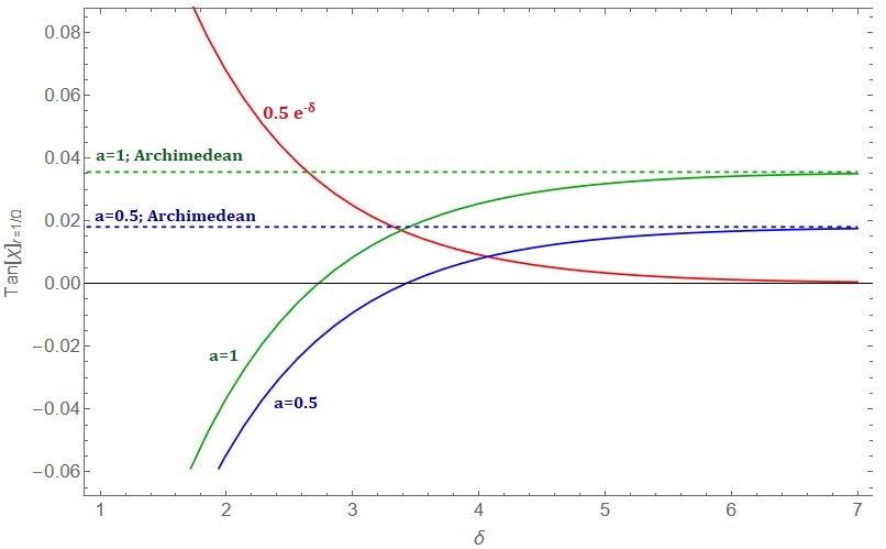
Figure 21: The ratio $\tan(\chi)=\beta_{\phi}/\beta_{r}$ (for high energy) at the outer light cylinder (in the flat case; i.e., $r=1/\Omega$) versus a free parameter $\delta$ to control the variation in the wire shape from the Archimedean case, for mass-rotation parameter $\eta=0.1$. The variation allowed range here is $\left(0,\frac{1}{2}\right]$, and presented as an exponentially decaying function of the parameter $\delta$, and is plotted in red. We have two sets of curves corresponding to two different wire shapes: the dashed lines correspond to the Archimedean spiral case, and the solid ones correspond to a spiral that is slightly different from the Archimedean one. The colors of the curves correspond to the values of the Kerr parameter: blue curves are for $a=0.5$ and green curves are for maximally spinning black hole case ($a=1$). For some variations, the curves meet the horizontal axis, meaning that the ratio is zero.

For plotting purposes, we consider the following possible values of the variation: $\delta(r=1/\Omega)\in\left(0,\frac{1}{2}\right]$. Moreover, we present these possible values in a form of an exponentially decaying function $e^{-\delta}/2$, where $\delta$ here is just a free parameter, not the variation. We choose the allowed values of $\{\eta,a\}$ based on the following constraints:

$$\eta<\frac{1}{a+2\sqrt{2}}<\frac{1}{2\sqrt{2}}<\frac{1}{2}\hskip 28.45274pt\eta\sqrt{\frac{(1-a\eta)}{(1+a\eta)^{3}}}<\frac{1}{3\sqrt{3}}$$ (E34)

We show in figure (21) that the small variation can cause the ratio in the Kerr case to approach zero at the flat-case light cylinder position. However, this might not be the case for bigger values of $\eta$; in that case, we expect the ratio to approach zero further a bit from the light cylinder (i.e., at some finite $r>1/\Omega$) because of the decaying nature of the ratio as a function of the radial coordinate $r$ in general.

Moreover, far away from the light cylinder, the ratio in the Kerr case becomes

$$\lim_{E\to\infty}\tan(\chi(r\gg 1/\Omega))\approx-\sqrt{\delta(\delta+2)}+\frac{1+\delta}{r\Omega}$$ (E35)

Thus,

$$\lim_{E\to\infty}\lim_{r\to\infty}\tan(\chi)=-\sqrt{\delta(\delta+2)}\approx-\sqrt{2\delta}$$ (E36)

Also, the Lorenta factor (relative to the observer at infinity) far away from the light cylinder for large energy is

$$\gamma_{\beta}\approx\frac{1+\delta}{\sqrt{\delta(\delta+2)}}\approx\frac{1}{\sqrt{2\delta}}\to\infty$$ (E37)

In spherical coordinates the position vector is

$$\vec{r}=r\hat{r}\hskip 28.45274pt\Rightarrow\hskip 28.45274pt\hat{V}^{0}=0,\>\hat{V}^{r}=r,\>\hat{V}^{\phi}=0\hskip 28.45274pt\Rightarrow\hskip 28.45274pt\hat{V}^{\mu}=r\delta^{\mu}_{r}$$ (E38)

$$(\boldsymbol{e}_{0})_{\mu}=\begin{pmatrix}-g_{00}&0&g_{0\phi}\end{pmatrix}\hskip 56.9055pt(\boldsymbol{e}_{0})_{\mu}=\begin{pmatrix}0&g_{rr}&0\end{pmatrix}\hskip 56.9055pt(\boldsymbol{e}_{0})_{\mu}=\begin{pmatrix}g_{0\phi}&0&g_{\phi\phi}\end{pmatrix}$$ (E39)

To get the coordinate components (i.e., $\mu=\{t,r,\phi\}$) of the orthonormal basis vectors, we first diagonalize the metric tensor and obtain (note $g_{0\phi}=\sqrt{\Delta-g_{00}g_{\phi\phi}}=\sqrt{\frac{r^{2}}{g_{rr}}-g_{00}g_{\phi\phi}}$ )

$$g_{\mu\nu}=\begin{pmatrix}-g_{00}&g_{0\phi}\\ g_{0\phi}&g_{\phi\phi}\end{pmatrix}\to g^{\prime}_{\mu\nu}=\begin{pmatrix}-g^{\prime}_{00}&0\\ 0&g^{\prime}_{\phi\phi}\end{pmatrix},$$ (E40)

Let us work it out first without diagonalization: The 1-form basis is (I don’t know how to cite this)(bernagozzi2013mathematical)

REVIEW THE BASIS VECTORS BEFORE NORMALIZATION: THE r-VECTOR IS PROBABLY WRONG!

$$\boldsymbol{e}^{r}=\frac{r}{\sqrt{\Delta}}d\boldsymbol{r}\iff\left(\boldsymbol{e}^{r}\right)_{\mu}=\frac{r}{\sqrt{\Delta}}\begin{pmatrix}0&1&0\end{pmatrix}\overset{\boldsymbol{e}^{r}\cdot\boldsymbol{e}_{r}=1}{\hskip 14.22636pt\Rightarrow\hskip 14.22636pt}\left(\boldsymbol{e}_{r}\right)^{\mu}=\frac{\sqrt{\Delta}}{r}\begin{pmatrix}0\\ 1\\ 0\end{pmatrix}$$ (E41)

$$\boldsymbol{e}^{1}=\frac{1}{r}\left(-ad\boldsymbol{t}+(r^{2}+a^{2})d\boldsymbol{\phi}\right)\iff\left(\boldsymbol{e}^{1}\right)_{\mu}=\frac{1}{r}\begin{pmatrix}-a&0&r^{2}+a^{2}\end{pmatrix}$$ (E42)

$$\boldsymbol{e}^{2}=\frac{\sqrt{\Delta}}{r}\left(d\boldsymbol{t}-ad\boldsymbol{\phi}\right)\iff\left(\boldsymbol{e}^{2}\right)_{\mu}=\frac{\sqrt{\Delta}}{r}\begin{pmatrix}1&0&-a\end{pmatrix}$$ (E43)

Define the corresponding vector basis to be

$$\left(\boldsymbol{e}_{1}\right)^{\mu}=\begin{pmatrix}x\\ 0\\ y\end{pmatrix}\hskip 28.45274pt\left(\boldsymbol{e}_{2}\right)^{\mu}=\begin{pmatrix}z\\ 0\\ w\end{pmatrix}$$ (E44)

From the relation ($\left(\boldsymbol{e}_{\mu}\right)\cdot\left(\boldsymbol{e}^{\nu}\right)=g_{\mu}^{\>\>\>\nu}=\delta_{\mu}^{\nu}$), we obtain

$$\left(\boldsymbol{e}_{r}\right)^{\mu}=\frac{\sqrt{\Delta}}{r}\begin{pmatrix}0\\ 1\\ 0\end{pmatrix}\hskip 28.45274pt\left(\boldsymbol{e}_{1}\right)^{\mu}=\frac{1}{r}\begin{pmatrix}a\\ 0\\ 1\end{pmatrix}\hskip 28.45274pt\left(\boldsymbol{e}_{2}\right)^{\mu}=\frac{1}{r\sqrt{\Delta}}\begin{pmatrix}r^{2}+a^{2}\\ 0\\ a\end{pmatrix}$$ (E45)

Using the relation $\hat{e}_{\mu}=\boldsymbol{e}_{\mu}/\sqrt{\left(\boldsymbol{e}_{\mu}\right)^{\nu}\left(\boldsymbol{e}_{\mu}\right)_{\nu}}\>$, we can normalize the orthogonal basis we have

$$\left(\hat{e}_{r}\right)^{\mu}=\left(\boldsymbol{e}_{r}\right)^{\mu}=\frac{\sqrt{\Delta}}{r}\begin{pmatrix}0\\ 1\\ 0\end{pmatrix}\hskip 28.45274pt\left(\hat{e}_{1}\right)^{\mu}=\left[1-\frac{2M^{2}}{r^{3}}a+\left(M^{2}+2M\frac{M^{2}-2M+2}{r}-1\right)\frac{a^{2}}{r^{2}}\right]^{-\frac{1}{2}}\frac{1}{r}\begin{pmatrix}a\\ 0\\ 1\end{pmatrix}$$ (E46)

$$\left(\hat{e}_{2}\right)^{\mu}=\left[-\alpha^{2}-\left(\alpha^{2}+4\frac{M^{2}}{r}-M^{2}\left(1+\frac{2M}{r}\right)\right)\frac{a^{4}}{r^{4}}+\left(r^{2}-4Mr-2r^{2}\alpha^{2}\right)\frac{a^{2}}{r^{4}}\right]^{-\frac{1}{2}}\frac{1}{r^{2}}\begin{pmatrix}r^{2}+a^{2}\\ 0\\ a\end{pmatrix}$$ (E47)

To make sure what we got is the correct basis, we just try to set $a=0$ and see if they reduce to the Schwarzshild case ($\Delta\overset{a=0}{\to}r^{2}\alpha^{2}$):

$$\left(\hat{e}_{r}\right)^{\mu}\to\alpha\begin{pmatrix}0\\ 1\\ 0\end{pmatrix}\hskip 28.45274pt\left(\hat{e}_{1}\right)^{\mu}\to\frac{1}{r}\begin{pmatrix}0\\ 0\\ 1\end{pmatrix}=\left(\hat{e}_{\phi}\right)^{\mu}\hskip 28.45274pt\left(\hat{e}_{2}\right)^{\mu}\to\frac{1}{\sqrt{-\alpha^{2}}}\begin{pmatrix}1\\ 0\\ 0\end{pmatrix}=\left(\hat{e}_{0}\right)^{\mu}$$ (E48)

$$\frac{D}{Dt}\hat{V}^{\mu}=\left(1-r\frac{d}{dr}\ln(|\boldsymbol{e}_{\mu}|)\right)v^{r}\delta^{\mu}_{r}+r\left(\Gamma^{\mu}_{r0}+\Gamma^{\mu}_{rr}v^{r}+\Gamma^{\mu}_{r\phi}v^{\phi}\right)$$ (E49)

$$\frac{D}{Dt}\hat{V}^{\mu}=v^{r}\left(\delta_{r}^{\mu}+r\left(\Gamma^{\mu}_{rr}-\delta_{r}^{\mu}\frac{1}{2}\frac{d}{dr}\ln(g_{\mu\mu})\right)\right)+r\left(\Gamma^{\mu}_{r0}+\Gamma^{\mu}_{r\phi}v^{\phi}\right)$$ (E50)

At the same limits, we have

$$\beta_{\phi}\hskip 7.11317pt\overset{a=0}{=}\hskip 7.11317ptr\Omega\alpha\left(1-\frac{2r^{2}\Omega_{1}(r)^{2}}{\alpha^{2}+r^{2}\Omega_{1}(r)^{2}}\right)$$ (E51)

We also expand in small $\delta$ at the actual light cylinder in the Schwarzshild case $(r=r_{2})_{a=0}$.

$$\tan(\chi;{E\to\infty})_{r=r_{2}}=\frac{1}{2}\left(\frac{\alpha}{r\Omega_{1}(r)}-\frac{r\Omega_{1}(r)}{\alpha}\right)\approx-\frac{r_{2}\Omega}{2\alpha}\left(\left(1-\frac{\alpha^{2}}{r_{2}^{2}\Omega^{2}}\right)+\left(1+\frac{\alpha^{2}}{r_{2}^{2}\Omega^{2}}\right)\delta\right)$$ (E52)

We obtain in the case of Schwarzshild metric (expanding in small $\delta$) around the flat-case light cylinder ($r\approx 1/\Omega$)

$$\tan(\chi)\approx\frac{1}{2}\left(\alpha-\frac{1}{\alpha}\right)\overset{r\gg 1/\Omega}{\approx}-\frac{M}{r}$$ (E53)

So, it approaches zero quickly after the light cylinder, as we see this graphically.

$$\delta\to\frac{1}{2}e^{-\delta}\hskip 28.45274pt\Rightarrow\hskip 28.45274pt\Omega_{1}(1/\Omega)\approx\Omega\left(1+\frac{1}{2}e^{-\delta}\right)$$ (E54)

we can find a small change $\delta\Omega$ to the shape so that it reaches zero. Moreover, in a few light-cylinder radii, we can see that the ratio goes to zero.

$$\tan(\chi)\approx\frac{\Omega_{1}(r)-E\sqrt{\Omega_{1}(r)^{2}-\Omega^{2}}}{r\Omega^{2}}+\frac{M\Omega_{1}(r)\left(3aM\Omega-1\right)}{r^{2}\Omega^{2}}\hskip 5.69046pt\overset{\Omega_{1}(r)\approx\Omega}{\approx}\hskip 5.69046pt\frac{1}{r\Omega}+\frac{3aM}{r^{2}}-\frac{1}{r^{2}\Omega}\hskip 5.69046pt\overset{r\to\infty}{\to}\hskip 5.69046pt0$$ (E55)

Thus, the dominant component of the velocity is the radial one:

$$\beta_{r}\approx\frac{\Omega}{\Omega_{1}(r)}\alpha^{2}\hskip 5.69046pt\overset{\Omega_{1}(r)\approx\Omega}{\approx}\hskip 5.69046pt\alpha^{2}\hskip 5.69046pt\overset{r\to\infty}{\to}\hskip 5.69046pt1$$ (E56)

For infinite energy, we have

$$tan(\chi)\overset{r\to\infty}{\approx}-\sqrt{\left(\frac{\Omega_{1}(r)}{\Omega}\right)^{2}-1}\overset{\Omega_{1}\approx\Omega}{\approx}0$$ (E57)

Next, we calculate the Lorentz factors relative to fixed observers in spacetime and co-rotating observers with the wire. The Lorentz factor can be used to get the speed of the particle as a function of the distance from the black hole singularity. This speed will never exceed the speed of light, unlike the proper speed in (B17), see figure (22). We construct the Lorentz factor in curved spacetimes by imagining filling the (2+1)-D Kerr spacetime with momentarily fixed observers everywhere (only between the ergosphere and the outer light cylinder, as we will show why later). The particle anywhere between the light cylinders is at the same location as exactly one of these observers. At this point, we can obtain a dot product between the four-velocity of the fixed observer and that of the particle, and get an invariant quantity, which is the Lorentz factor of the particle as seen by the fixed observer where the particle is. The four-velocity of a fixed observer is ($\dot{t}\geq 0,\dot{r}=0,\dot{\phi}=0$)

$$U^{\mu}_{fixed}=\begin{pmatrix}\dot{t}\\ 0\\ 0\end{pmatrix}\xrightarrow[\mathcal{L}=-1]{\mathcal{L}=-g_{00}\,\dot{t}^{2}}U^{\mu}_{fixed}=\frac{1}{\sqrt{g_{00}\,}}\begin{pmatrix}1\\ 0\\ 0\end{pmatrix}\Rightarrow U_{\mu}^{fixed}=\begin{pmatrix}-\sqrt{g_{00}\,}&&0&&\frac{g_{0\phi}\,}{\sqrt{g_{00}\,}}\end{pmatrix}$$ (E58)

The four-velocity of the particle is

$$U^{\mu}_{particle}=\begin{pmatrix}\dot{t}\\ \dot{r}\\ \dot{\phi}\end{pmatrix}=\begin{pmatrix}\dot{t}\\ \dot{r}\\ \Phi^{\prime}(r)\dot{r}+\Omega\dot{t}\end{pmatrix}$$ (E59)

The relative Lorentz factor observed by such fixed observes for the particle is

$$\gamma=-U_{\mu}^{fixed}U^{\mu}_{particle}=\left(\sqrt{g_{00}\,}-\frac{\Omega g_{0\phi}\,}{\sqrt{g_{00}\,}}\right)\dot{t}-\frac{\Phi^{\prime}(r)g_{0\phi}\,}{\sqrt{g_{00}\,}}\dot{r}$$ (E60)

From both (B2) and (B17), the Lorentz factor becomes

$$\gamma=\left(\sqrt{g_{00}\,}-\frac{\Omega g_{0\phi}\,}{\sqrt{g_{00}\,}}\right)\frac{E}{G_{00}\,}\pm\\ \left(\left(\sqrt{g_{00}\,}-\frac{\Omega g_{0\phi}\,}{\sqrt{g_{00}\,}}\right)\frac{G_{0r}\,}{G_{00}\,}-\frac{\Phi^{\prime}(r)g_{0\phi}\,}{\sqrt{g_{00}\,}}\right)\sqrt{\frac{E^{2}-G_{00}\,}{G_{0r}^{2}+G_{00}\,G_{rr}\,}}$$ (E61)

The negative (positive) sign means that the particle is moving towards (away from) the black hole. This Lorentz factor is only defined whenever $g_{00}$ is positive; i.e., outside the ergosphere

$$\mathcal{R}=M\left(1+\sqrt{1-a^{2}\cos^{2}{\theta}}\right)$$ (E62)

See Fig. 22 for a plot of the speed of the particle observed by the fixed observers, which can be obtained from the relation

$$\gamma=\frac{1}{\sqrt{1-v^{2}}}$$ (E63)

We have a range of allowed values for the constant of motion $E$. Let $r_{1}$ and $r_{2}$ be the locations of the light cylinders. From (B17), we get

$$0<G_{00}\,\leq E^{2},\hskip 85.35826ptr\in(r_{1},r_{2})$$ (E64)

$$\Omega^{2}r^{3}-(1-a^{2}\eta^{2}-E^{2})r+2M(1-a\eta)^{2}\geq 0$$ (E65)

This is a cubic equation on the form $\Omega^{\,2}r^{3}-br+d=0$ that has to be always non-negative, for all the positive values of $r$. Therefore, we need to guarantee that the minimum (i.e., extreme) value of the cubic function is also non-negative. We obtain

$$\Omega^{\,2}r^{3}-br+d\geq 0,\hskip 56.9055ptb>0,\>d\geq\frac{1}{3\sqrt{3}}\>\frac{2b^{\frac{3}{2}}}{\Omega}$$ (E66)

$$\left\{\begin{array}[]{cc}\sqrt{1-a^{2}\eta^{2}-3\eta^{\frac{2}{3}}(1-a\eta)^{\frac{4}{3}}}\leq E&r\in(r_{1},r_{2})\\ 0\leq E<\infty&r>r_{2}\end{array}\right.$$ (E67)

The time constant $E$ that appears in (E61) can be related to the initial conditions as observed by a set of fixed observers along the rotating wire. We imagine a set of fixed observers along the rotating wire, only defined between the two light cylinders, and they observe the particle radial speed only. We obtain the relative Lorentz factor as seen by the observers along the wire by applying the same procedure we used to get (E61), but now on the (1+1)-D sub-manifold. The four-velocity of a fixed observer is ($\dot{t}\geq 0,\dot{r}=0$)

$$U^{\mu}_{fixed}=\begin{pmatrix}\dot{t}\\ 0\end{pmatrix}\xrightarrow[\mathcal{L}=-1]{\mathcal{L}=-G_{00}\,\dot{t}^{2}}U^{\mu}_{fixed}=\frac{1}{\sqrt{G_{00}\,}}\begin{pmatrix}1\\ 0\end{pmatrix}\Rightarrow U_{\mu}^{fixed}=\begin{pmatrix}-\sqrt{G_{00}\,}&&\frac{G_{0r}\,}{\sqrt{G_{00}\,}}\end{pmatrix}$$ (E68)

The four-velocity of the particle is

$$U^{\mu}_{particle}=\begin{pmatrix}\dot{t}\\ \dot{r}\end{pmatrix}\hskip 28.45274pt\xrightarrow[]{(\ref{tDOT})}\hskip 28.45274ptU^{\mu}_{particle}=\begin{pmatrix}\frac{G_{0r}\,\dot{r}+E}{G_{00}\,}\\ \dot{r}\end{pmatrix}$$ (E69)

The radial Lorentz factor of the radially moving particle relative to the fixed observers (on the wire) is the invariant quantity

$$\gamma_{r}=-U_{\mu}^{fixed}U^{\mu}_{radial}=\frac{E}{\sqrt{G_{00}\,}}=\frac{1}{\sqrt{1-v_{r}^{2}}}$$ (E70)

As expected, the radial Lorentz factor coincides with the total one in (E61) in the case of a non-rotating wire:

$$\gamma=\gamma_{r}=\frac{E}{\sqrt{G_{00}}}=\frac{E}{\sqrt{g_{00}}}\hskip 113.81102pt(\Omega=0)$$ (E71)

Since the Lorentz factor is always positive, the constant $E$ is always positive too. We can get $E$ easily from the initial conditions as seen by a fixed observer along the wire. If such an observer is at $r_{0}$ observes the particle moving along the wire a radial Lorentz factor $\gamma_{r0}$, we obtain

$$E=\gamma_{r}\sqrt{G_{00}}=\gamma_{r0}\sqrt{G_{00}(r_{0})}$$ (E72)

Hence, the invariant radial speed becomes

$$v_{r}(r)=\pm\sqrt{1-\frac{G_{00}\,}{E^{2}}}=\pm\sqrt{1-\left(\frac{1-v_{r\,0}^{2}}{G_{00}(r_{0})}\right)G_{00}}\hskip 28.45274ptr,r_{0}\in(r_{1},r_{2})$$ (E73)

Again, the sign determines the radial direction of motion of the particle (towards/outwards the black hole). We can easily see that this speed does not exceed the speed of light, see Fig. (22). Since the metric function $G_{00}$ does not depend on the shape of the wire (the function $\Phi$), this interesting result means that the radial speed of the particle does not depend on the shape of the wire (but it depends on its angular speed). The Lorentz factor in (E61) becomes

$$\gamma=\frac{E}{G_{00}}\left[\left(\sqrt{g_{00}}-\frac{\Omega g_{0\phi}}{\sqrt{g_{00}}}\right)\pm\frac{v_{r}}{\sqrt{G_{0r}^{2}+G_{00}\,G_{rr}}}\left(\left(\sqrt{g_{00}}-\frac{\Omega g_{0\phi}}{\sqrt{g_{00}}}\right)G_{0r}-\frac{\Phi^{\prime}(r)g_{0\phi}}{\sqrt{g_{00}}}G_{00}\right)\right]\\ =\frac{\gamma_{r}}{\sqrt{G_{00}}}\left[\left(\sqrt{g_{00}}-\frac{\Omega g_{0\phi}}{\sqrt{g_{00}}}\right)\pm\frac{v_{r}}{\sqrt{G_{0r}^{2}+G_{00}\,G_{rr}}}\left(\left(\sqrt{g_{00}}-\frac{\Omega g_{0\phi}}{\sqrt{g_{00}}}\right)G_{0r}-\frac{\Phi^{\prime}(r)g_{0\phi}}{\sqrt{g_{00}}}G_{00}\right)\right]$$ (E74)

$$\gamma=\gamma_{r0}\>\frac{\sqrt{G_{00}(r_{0})}}{G_{00}\,}\left(\sqrt{g_{00}\,}-\frac{\Omega g_{0\phi}\,}{\sqrt{g_{00}\,}}\right)\pm\\ \left(\left(\sqrt{g_{00}\,}-\frac{\Omega g_{0\phi}\,}{\sqrt{g_{00}\,}}\right)\frac{G_{0r}\,}{G_{00}\,}-\frac{\Phi^{\prime}(r)g_{0\phi}\,}{\sqrt{g_{00}\,}}\right)\sqrt{\frac{\gamma_{r0}^{2}G_{00}(r_{0})-G_{00}\,}{G_{0r}^{2}+G_{00}\,G_{rr}\,}}$$ (E75)

We imagine ejecting the particles on the outer light cylinder ($r=r_{2}$) with an initial Lorentz factor $\gamma_{0}$ as the initial conditions. Then, we solve for the energy $E$:

$$\gamma_{0}=\lim_{r\to r_{2}}\gamma=\frac{1}{2E}\left(\sqrt{g_{00}\,}-\frac{\Omega g_{0\phi}\,}{\sqrt{g_{00}\,}}\right)_{r_{2}}\left(1+G_{rr}\left(\frac{E}{G_{0r}}\right)^{2}\right)_{r_{2}}-\left(\frac{\Phi^{\prime}(r)g_{0\phi}}{\sqrt{g_{00}}}\frac{E}{|G_{0r}|}\right)_{r_{2}}$$ (E76)

$$E=\left\{\frac{\gamma_{0}\pm\sqrt{\gamma_{0}^{2}-\left(\sqrt{g_{00}\,}-\frac{\Omega g_{0\phi}\,}{\sqrt{g_{00}\,}}\right)\left[\left(\sqrt{g_{00}\,}-\frac{\Omega g_{0\phi}\,}{\sqrt{g_{00}\,}}\right)\frac{G_{rr}}{G_{0r}^{2}}-\frac{2}{|G_{0r}|}\frac{\Phi^{\prime}(r)g_{0\phi}}{\sqrt{g_{00}}}\right]}}{\left(\sqrt{g_{00}\,}-\frac{\Omega g_{0\phi}\,}{\sqrt{g_{00}\,}}\right)\frac{G_{rr}}{G_{0r}^{2}}-\frac{2}{|G_{0r}|}\frac{\Phi^{\prime}(r)g_{0\phi}}{\sqrt{g_{00}}}}\right\}_{r_{2}}$$ (E77)

Therefore, we see that there has to be a minimum initial Lorentz factor for the constant $E$ to have real values. Moreover, we only need the larger energy of the two solutions to guarantee that we have a solution between the light cylinders as well, by being consistent with the constraints (E90). Usually, we have a large Lorentz factor when the particle reaches the outer light cylinder; thus, giving the particle an initial push at the outer light cylinder with a relatively large $\gamma_{0}$ will result in a large amount of the energy:

$$E\approx\gamma_{0}\left(\frac{2G_{0r}^{2}}{\left(\sqrt{g_{00}\,}-\frac{\Omega g_{0\phi}\,}{\sqrt{g_{00}\,}}\right)G_{rr}-2|G_{0r}|\frac{\Phi^{\prime}(r)g_{0\phi}}{\sqrt{g_{00}}}}\right)_{r_{2}}\sim\gamma_{0}$$ (E78)

For large values of the Lorentz factor of the particle at the outer light cylinder, the energy of the particle behaves the same way as the Lorentz factor of the particle at the outer light cylinder. For the sake of plotting the speeds we got so far, which are merely functions of the radial coordinate $r$, it is better to make the radial coordinate dimensionless. We divide the radial coordinate by an arbitrary length $l$, which we set later to be the Kerr black hole horizon. The following transformation leads to only the changes

$$r\to\frac{r}{l}\hskip 28.45274pt\Rightarrow\hskip 28.45274pt\begin{array}[]{cc}g_{rr}(r)\to g_{rr}\left(r/l\right)/l^{2}\\ \Phi^{\prime}(r)\to\Phi^{\prime}(r/l)/l\end{array}\hskip 28.45274pt\Rightarrow\hskip 28.45274pt\begin{array}[]{cc}G_{rr}(r)\to G_{rr}\left(r/l\right)/l^{2}\\ G_{0r}(r)\to G_{0r}\left(r/l\right)/l\end{array}$$ (E79)

TRY

$$r\to\frac{r}{l}\hskip 28.45274pt\Rightarrow\hskip 28.45274pt\begin{array}[]{cc}g_{rr}(r)\to l^{2}\>g_{rr}\left(r/l\right)\\ \Phi^{\prime}(r)\to l\>\Phi^{\prime}(r/l)\end{array}\hskip 28.45274pt\Rightarrow\hskip 28.45274pt\begin{array}[]{cc}G_{rr}(r)\to l^{2}\>G_{rr}\left(r/l\right)\\ G_{0r}(r)\to l\>G_{0r}\left(r/l\right)\end{array}$$ (E80)

The speeds we obtained before become the following. Again, we suppress the notation of function in an argument: all the metrics components are evaluated at the dimensionless quantity $r/l$ unless otherwise specified.

$$\dot{r}=\pm\;l\;\sqrt{\frac{E^{2}-G_{00}\,}{G_{0r}^{2}+G_{00}\,G_{rr}\,}}$$ (E81)

$$\beta_{r}=l\>G_{00}\,\left(G_{0r}\,\pm E\sqrt{\frac{G_{0r}^{2}+G_{00}\,G_{rr}\,}{E^{2}-G_{00}\,}}\right)^{-1}$$ (E82)

The Lorentz factors standstill in this change.

$$\gamma=\gamma_{0}\>\frac{\sqrt{G_{00}(r_{0})}}{G_{00}\,}\left(\sqrt{g_{00}\,}-\frac{\Omega g_{0\phi}\,}{\sqrt{g_{00}\,}}\right)\pm\\ l\>\left(\left(\sqrt{g_{00}\,}-\frac{\Omega g_{0\phi}\,}{\sqrt{g_{00}\,}}\right)\frac{G_{0r}\,}{l\>G_{00}\,}-\frac{\Phi^{\prime}(r)g_{0\phi}\,}{l\>\sqrt{g_{00}\,}}\right)\sqrt{\frac{\gamma_{0}^{2}G_{00}(r_{0})-G_{00}\,}{G_{0r}^{2}+G_{00}\,G_{rr}\,}}$$ (E83)

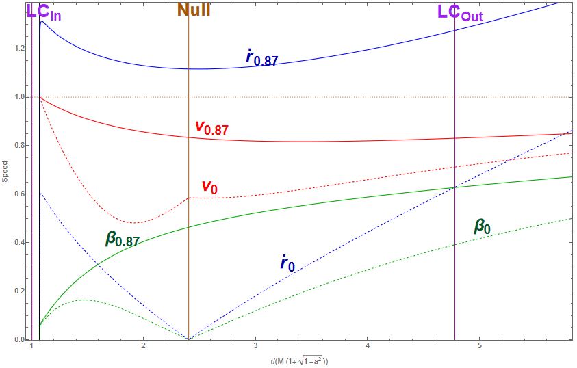
Figure 22: Various velocities for a particle moving in Kerr black hole, in the equatorial plane for Kerr parameter $a=0.5$ and mass-rotation parameter $\eta=0.1$. The coordinate $r$ here is taken relative to the Kerr horizon $M(1+\sqrt{1-a^{2}})$. We have two sets of curves corresponding to two different initial Lorentz factors $\gamma_{r0}$ in (E73) at the null line: the dashed curves correspond to a zero initial speed ($\gamma_{r0}=1$), and the solid ones correspond to an initial speed of 0.87 of the speed of light ($\gamma_{r0}\approx 2.03)$. The colors of the curves correspond to the different kinds of speeds: (i) blue curves are the proper speed, $\dot{r}$ in (B17); (ii) green curves are speed $\beta_{r}$, the speed measured by an observer at infinity (iii) red curves are the speed correspond to the Lorentz factor in (E75). The dotted (brown) horizontal line at $1$ is plotted to indicate the speed of light (we see that $dr/d\tau$ exceeds the speed of light between the two light cylinders, while the other two speeds do not). The vertical lines are colored as follows: purple for both light cylinders (the inner one is so close to the Kerr horizon at 1); brown for the null line, which lies between the light cylinders; and, black for the ergosphere (E62). The ergosphere lies before the null line due to a condition on both $\eta,\>a$, in addition to the condition (E19): $|a-\eta^{-1}|>2\sqrt{2}$. Finally, we only plotted the speeds outside the ergosphere ($\mathcal{R}=2M$ here) because the Lorentz factor in (E75) is only defined after such radius.

From (E87), we see that $E$ is strictly positive. We can also verify that from the constraints in (E19):

$$\eta^{\frac{2}{3}}\frac{(1-a\eta)^{\frac{1}{3}}}{1+a\eta}<\frac{1}{3}\iff 3\eta^{\frac{2}{3}}\frac{(1-a\eta)^{\frac{4}{3}}}{1-a^{2}\eta^{2}}<1\iff 0<1-a^{2}\eta^{2}-3\eta^{\frac{2}{3}}(1-a\eta)^{\frac{4}{3}}$$ (E84)

E.1 The Null Line

We are looking for the position where both the gravitational pulling of the rotating spacetime (i.e., curvature) balances the repulsion from the rotation of the wire. We call this location the null line. As we are going to show, it is also the location where $G_{00}$ has its extremum. Let the null line be located at $R_{0}$ distance from the black hole, and between the two light cylinders. For a stationary particle at $r=R_{0}$ to remain in place, we demand the speed and acceleration of the coordinate $r$ to vanish. Notice that the metric functions are always non-zero in the region between the two light cylinders; so, we get

$$\ddot{r}(R_{0})=0\hskip 28.45274pt\xrightarrow[G_{00}(R_{0})=E^{2}]{\dot{r}(R_{0})=0}\hskip 28.45274pt\partial_{r}G_{00}(R_{0})=0\hskip 28.45274ptR_{0}\in(r_{1},r_{2})$$ (E85)

$$R_{0}=M\eta^{-\frac{2}{3}}(1-a\eta)^{\frac{2}{3}}=$$ (E86)

The result makes sense because the null radius is expected to increase when either the mass of the black hole (i.e., the gravitational pulling) increases or the rotation parameter of either the black hole or the sub-manifold decreases.

E.2 Constraints

E.2.1 The Time Constant Constraints

The constant of motion $E$ has a constrained range of values. From either (B17) or (E73), we get

$$0<G_{00}\,\leq E^{2},\hskip 85.35826ptr\in(r_{1},r_{2})$$ (E87)

$$\Omega^{2}r^{3}-(1-a^{2}\eta^{2}-E^{2})r+2M(1-a\eta)^{2}\geq 0$$ (E88)

This is a cubic equation on the form we had in (E6), but this time it has to be always non-negative, for all the positive values of $r$. Therefore, we need to guarantee that the minimum value of the cubic function is also non-negative. Similar to the constraints in (E10), we proceed as we did before with the cubic equation (E6) and get constraints on the time constant:

$$\Omega^{\,2}r^{3}-br+d\geq 0,\hskip 56.9055ptb>0,\>d\geq\frac{1}{3\sqrt{3}}\>\frac{2b^{\frac{3}{2}}}{\Omega}$$ (E89)

$$\left\{\begin{array}[]{cc}0<\sqrt{1-a^{2}\eta^{2}-3\eta^{\frac{2}{3}}(1-a\eta)^{\frac{4}{3}}}\leq E<\sqrt{1-a^{2}\eta^{2}}&:\eta\neq 0\\ 1\leq E&:\eta=0\end{array}\right.$$ (E90)

From (E87), we see that $E$ is strictly positive. We can also verify that from the constraints in (E19):

$$\eta^{\frac{2}{3}}\frac{(1-a\eta)^{\frac{1}{3}}}{1+a\eta}<\frac{1}{3}\iff 3\eta^{\frac{2}{3}}\frac{(1-a\eta)^{\frac{4}{3}}}{1-a^{2}\eta^{2}}<1\iff 0<1-a^{2}\eta^{2}-3\eta^{\frac{2}{3}}(1-a\eta)^{\frac{4}{3}}$$ (E91)

E.2.2 The Invariant Radial Speed Constraints

We obtained the set of values that the time constant $E$ only take; consequently, from (E72), we can obtain the set of allowed values to the (initial) radial speed as observed by the fixed observers along the string. Furthermore, as a check for the result (E86), we are going to show that this initial speed vanishes and remains zero only if the particle is at the null line. From (E90), (E72), and (E73), we get

$$1-\frac{1-a^{2}\eta^{2}-3\eta^{\frac{2}{3}}(1-a\eta)^{\frac{4}{3}}}{G_{00}}\leq v^{2}(r)<1-\frac{1-a^{2}\eta^{2}}{G_{00}}$$ (E92)

$$1-\frac{1-a^{2}\eta^{2}-3\eta^{\frac{2}{3}}(1-a\eta)^{\frac{4}{3}}}{G_{00}(r_{0})}\leq v_{0}^{2}<1-\frac{1-a^{2}\eta^{2}}{G_{00}(r_{0})}$$ (E93)

A zero invariant radial speed is equivalent to the equality case of the inequality (E87)

$$G_{00}=E^{2}\iff\Omega^{2}r^{3}-(1-a^{2}\eta^{2}-E^{2})r+2M(1-a\eta)^{2}=0\hskip 28.45274ptr\in(r_{1},r_{2})$$ (E94)

IS THIS CORRECT?? $v(R_{0})=0\>but\>v_{0}(r_{0})>0\>and\>r_{0}>R_{0}$

This cubic equation is always non-negative from (E87). Nevertheless, we focus now on the special case that it is zero. Therefore, we just modify the constraints in (E89) to be

$$\Omega^{\,2}r^{3}-br+\frac{1}{3\sqrt{3}}\>\frac{2b^{\frac{3}{2}}}{\Omega}=0,\hskip 56.9055ptb>0$$ (E95)

Thus, the only case that this equation is zero is when its minimum is zero. From (E7), the minimum radius is

$$r_{min}=\sqrt{\frac{b}{3\Omega^{2}}}=\sqrt{\frac{1-a^{2}\eta^{2}-E^{2}}{3\Omega^{2}}}\hskip 28.45274pt\xrightarrow[(\ref{NullLine})]{(\ref{AllConstraints})}\hskip 28.45274ptr_{min}\in(0,R_{0}]$$ (E96)

Since the fixed observers along the string are only defined between the two light cylinders as well as the null line, the invariant radial speed is also defined in the same domain. Therefore, we are restricted to only work with the cases where $r_{min}$ is defined between the two light cylinders.

$$v(r_{min})=0\hskip 85.35826ptr_{min}\in(r_{1},R_{0}]$$ (E97)

IGNORE THIS TEXT Let us apply some initial conditions. We place a particle on the null line with the initial Lorentz factor $\gamma_{0}$ along the 1-D path it will follow. Let us calculate the Energy from (LABEL:EnergyConstraintsInGeneral). If we start with zero initial radial speed, we get

$$E=\frac{G_{00}(r_{0})}{\sqrt{A_{1}(r_{0})}-\frac{\Omega G_{1}(r_{0})}{A_{1}(r_{0})}}=\frac{E^{2}}{\sqrt{A_{1}(r_{0})}-\frac{\Omega G_{1}(r_{0})}{A_{1}(r_{0})}}$$ (E98)

THEN WHAT??? This result does not make any sense because $v_{0}$ must be zero always! What is the meaning of having non-zero radial speed everywhere if we start with such initial conditions???

These fixed observers are not fixed relative to the (2+1)-D manifold of an observer with the Kerr metric. So, we have to find out a way to solve this. Here is a suggestion

The fixed observers are also rotating observers (from the prospective of the (2+1)-D Kerr observers) according to the equation

$$\dot{\phi}=\frac{d\phi}{d\tau}=\frac{d\phi/dt}{d\tau/dt}=\Omega\dot{t}$$ (E99)

And they have a four-velocity vector of

$$U^{\mu}_{rot}=\dot{t}\begin{pmatrix}1\\ 0\\ \Omega\end{pmatrix}\xrightarrow[\mathcal{L}=-1,\>\dot{\phi}=\Omega\dot{t}]{\mathcal{L}=g_{00}\,\dot{t}^{2}+g_{\phi\phi}\,\dot{\phi}^{2}+2g_{0\phi}\,\dot{t}\dot{\phi}}U^{\mu}_{rot}=\frac{1}{\sqrt{G_{00}\,}}\begin{pmatrix}1\\ 0\\ \Omega\end{pmatrix}$$ (E100)

These rotating observers see a particle that moves with

$$\gamma_{1}(r)=\gamma(r_{0})\sqrt{\frac{G_{00}(r_{0})}{G_{00}\,}}$$ (E101)

Let us get the relative Lorentz factor of the rotating observers as seen by fixed observers (both in the Kerr metric). For the fixed observers,

$$U_{\mu}^{fixed}=\begin{pmatrix}g_{00}\,&&0&&g_{0\phi}\,\end{pmatrix}$$ (E102)

The fixed observers see the rotating ones (both in the Kerr metric) move with a relative Lorentz factor of

$$\gamma_{2}(r)=-U_{\mu}^{fixed}U^{\mu}_{rot}=\frac{-g_{00}\,-\Omega g_{0\phi}\,}{G_{00}\,}$$ (E103)

We calculate the following when the particle, the rotating observers of the Kerr, and the fixed observers of the Kerr all are at the same point of spacetime. We can get the relative Lorentz factor of the particle as seen by the fixed observers of the Kerr.

I DO NOT THINK THAT THIS IS IMPORTANT Note that

$$v(r_{0})\geq 1\Rightarrow v(r)\geq 1$$ (E104)

SUBTLETY IS HERE: Why do we have a required initial minimum speed?

In case the initial speed is less than unity (the speed of light), we note that the second term is negative, with a minimum negative value occurs when the initial speed is zero. At this point, we have the following constraint (or otherwise the observed velocity will be imaginary)

$$G_{00}\,\leq G_{00}(r_{0})$$ (E105)

We know that at the null point $r_{0}=\eta^{-\frac{2}{3}}$, this condition is always satisfied. So,

Rewriting (LABEL:ObservedVelocityCompleted) in a more standard form

$$\gamma(r)=\gamma_{0}\sqrt{\frac{G_{00}(r_{0})}{G_{00}\,}}$$ (E106)

In the specific case of the metric we have been using, while starting from the null point, we get

$$\gamma(r)=\gamma_{0}\sqrt{\frac{G_{00}(r_{0})}{G_{00}\,}}\hskip 56.9055ptr_{0}=\eta^{-\frac{2}{3}}$$ (E107)

We will set the boundaries we have on the time constant in terms of the spacetime parameters (and others) and get back to this equation to talk about the boundaries on the initial Lorentz factor, if there is any (of course we should get $v(r_{0})<1$ is a must).

DO WE NEED THIS?

Back to equation (LABEL:ObservedVelocityCompleted), we have a constraint on the initial speed as follows: we are sure that it does not exceed the speed of light because $G_{00}(r_{0})>0$; so, it has a minimum of zero that does not attain. Then, we have

$$G_{00}(r_{0})<0\Rightarrow 1+3\eta^{\frac{2}{3}}G_{00}(r_{0})<1$$ (E108)

Moreover, we have an upper bound to that function

$$G_{00}\,\leq 1-3\eta^{\frac{2}{3}}\iff 3\eta^{\frac{2}{3}}\leq 1+G_{00}\,$$ (E109)

Thus,

$$\left\{\begin{array}[]{cc}3\eta^{\frac{2}{3}}\leq 1+G_{00}(r_{0})\leq v^{2}(r_{0})\leq 1-3\eta^{\frac{2}{3}}G_{00}(r_{0})<1,\hskip 14.22636pt\eta<\frac{1}{3\sqrt{3}}&:\eta\neq 0\\ 0\leq 1+G_{00}(r_{0})\leq v^{2}(r_{0})<1&:\eta=0\end{array}\right.$$ (E110)

Generally speaking,

$$\boxed{3\eta^{\frac{2}{3}}\leq v^{2}(r_{0})<1}$$ (E111)

If the initial invariant radial speed at the null line (E86) is zero, the final one there is zero too. From (E72),

$$v_{0}(R_{0})=0\iff E^{2}=G_{00}(R_{0})=1-a^{2}\eta^{2}-3\eta^{\frac{2}{3}}(1-a\eta)^{\frac{4}{3}}\mbox{}$$

$$v(r)=0\iff G_{00}(r)=E^{2}=G_{00}(R_{0})$$ (E112)

Then, we conclude that $r=R_{0}$: the particle remains at the null line.

E.3 Plots

Figure 23: Different velocities for a particle moving in Schwarzschild black hole, in equatorial plane, Kerr parameter $a=0$, mass-rotation parameter $\eta=0.1$. Two sets of curves (blue, green, and brown) correspond to different invariant radial Lorentz speeds at the null line: a zero speed for dashed curves and a speed of 0.7 of the speed of light ($\gamma_{0}\sim 1.4)$ for solid curves. Different curves correspond to: (i) blue curves are the proper speed, $dr/d\tau$, speed of the coordinate $r$ w.r.t. to the proper time of the particle; (ii) brown curves are the invariant (total) speed $v=\sqrt{1-\frac{1}{\gamma^{2}}}$, Eq. (E75); (iii) green curves are the invariant radial speed, Eq. (E73), which is only defined between the two light cylinders. The dotted horizontal line at $1$ is plotted to indicate the speed of light ($dr/d\tau$ can exceed the speed of light between the two light cylinders). The inner and outer light cylinders are the two purple vertical lines, and the null line is the red one, all at different locations compared to Fig. (22).

E.4

Rotating Kerr

$$\Sigma=\sqrt{\left(a^{2}M^{2}+r^{2}\right)^{2}-a^{2}M^{2}\sin^{2}(\theta)\left(a^{2}M^{2}-2Mr+r^{2}\right)}\mbox{}$$

$$\Delta=a^{2}M^{2}-2Mr+r^{2}\mbox{}$$

$$g_{00}=-1+\frac{\Omega^{2}\sin^{2}(\theta)\left(\left(a^{2}M^{2}+r^{2}\right)^{2}-a^{2}\Delta M^{2}\sin^{2}(\theta)\right)}{\Sigma}+\frac{4aM^{2}r\Omega\sin^{2}(\theta)}{\Sigma}+\frac{2Mr}{\Sigma}$$ (E113)

Figure 24: Inner and outer light cylinder and null surface for Kerr black hole in the equatorial plane, with angular velocity of field lines $\Omega=0.3$.

References

- Bardeen et al. (1972) Bardeen, J. M., Press, W. H., & Teukolsky, S. A. 1972, ApJ, 178, 347
- Barkov & Komissarov (2008) Barkov, M. V., & Komissarov, S. S. 2008, MNRAS, 385, L28
- Beskin (2009) Beskin, V. S. 2009, MHD Flows in Compact Astrophysical Objects: Accretion, Winds and Jets
- Beskin et al. (1992) Beskin, V. S., Istomin, Y. N., & Parev, V. I. 1992, Soviet Ast., 36, 642
- Beskin & Kuznetsova (2000) Beskin, V. S., & Kuznetsova, I. V. 2000, Nuovo Cimento B Serie, 115, 795
- Bicknell & Begelman (1996) Bicknell, G. V., & Begelman, M. C. 1996, ApJ, 467, 597
- Birdsall & Langdon (1991) Birdsall, C. K., & Langdon, A. B. 1991, Plasma Physics via Computer Simulation
- Blandford et al. (2019) Blandford, R., Meier, D., & Readhead, A. 2019, ARA&A, 57, 467
- Blandford & Königl (1979) Blandford, R. D., & Königl, A. 1979, ApJ, 232, 34
- Blandford & Payne (1982) Blandford, R. D., & Payne, D. G. 1982, MNRAS, 199, 883
- Blandford & Znajek (1977) Blandford, R. D., & Znajek, R. L. 1977, MNRAS, 179, 433
- Boris & Roberts (1969) Boris, J. P., & Roberts, K. V. 1969, Journal of Computational Physics, 4, 552
- Camenzind (1986) Camenzind, M. 1986, A&A, 162, 32
- Chen & Beloborodov (2014) Chen, A. Y., & Beloborodov, A. M. 2014, ApJ, 795, L22
- Clausen-Brown et al. (2011) Clausen-Brown, E., Lyutikov, M., & Kharb, P. 2011, MNRAS, 415, 2081
- Comisso & Asenjo (2021) Comisso, L., & Asenjo, F. A. 2021, Phys. Rev. D, 103, 023014
- Contopoulos et al. (2020) Contopoulos, I., Pétri, J., & Stefanou, P. 2020, MNRAS, 491, 5579
- Crinquand et al. (2020) Crinquand, B., Cerutti, B., Philippov, A., Parfrey, K., & Dubus, G. 2020, Phys. Rev. Lett., 124, 145101
- Goldreich & Julian (1970) Goldreich, P., & Julian, W. H. 1970, ApJ, 160, 971
- Grad (1967) Grad, H. 1967, Physics of Fluids, 10, 137
- Gralla & Jacobson (2014) Gralla, S. E., & Jacobson, T. 2014, MNRAS, 445, 2500
- Gruzinov (2007) Gruzinov, A. 2007, arXiv e-prints, arXiv:0710.1875
- Hakobyan et al. (2022) Hakobyan, H., Philippov, A., & Spitkovsky, Anatoly, et al. 2022, arXiv e-prints, arXiv:2209.02121
- Hirotani & Okamoto (1998) Hirotani, K., & Okamoto, I. 1998, ApJ, 497, 563
- Kim et al. (2018) Kim, J. Y., Krichbaum, T. P., & Lu, R. S., et al. 2018, A&A, 616, A188
- Komissarov (2004) Komissarov, S. S. 2004, MNRAS, 350, 427
- Komissarov et al. (2009) Komissarov, S. S., Vlahakis, N., Königl, A., & Barkov, M. V. 2009, MNRAS, 394, 1182
- Krolik (1999) Krolik, J. H. 1999, Active galactic nuclei : from the central black hole to the galactic environment
- Landau & Lifshitz (1975) Landau, L. D., & Lifshitz, E. M. 1975, The classical theory of fields
- Levinson (2000) Levinson, A. 2000, Phys. Rev. Lett., 85, 912
- Levinson & Rieger (2011) Levinson, A., & Rieger, F. 2011, ApJ, 730, 123
- Lu et al. (2023) Lu, R.-S., Asada, K., & Krichbaum, Thomas P, et al. 2023, Nature, 616, 686
- Lyutikov (2003) Lyutikov, M. 2003, MNRAS, 346, 540
- Lyutikov (2009) —. 2009, MNRAS, 396, 1545
- Lyutikov (2022) —. 2022, ApJ, 933, L6
- Lyutikov et al. (2005) Lyutikov, M., Pariev, V. I., & Gabuzda, D. C. 2005, MNRAS, 360, 869
- McKinney (2006) McKinney, J. C. 2006, MNRAS, 368, 1561
- Michel (1969) Michel, F. C. 1969, ApJ, 158, 727
- Michel (1973) —. 1973, ApJ, 180, L133
- Misner et al. (1973) Misner, C. W., Thorne, K. S., & Wheeler, J. A. 1973, Gravitation (San Francisco: W.H. Freeman and Co., 1973)
- Nakamura & Asada (2013) Nakamura, M., & Asada, K. 2013, ApJ, 775, 118
- Nokhrina & Beskin (2017) Nokhrina, E. E., & Beskin, V. S. 2017, MNRAS, 469, 3840
- Philippov et al. (2015) Philippov, A. A., Spitkovsky, A., & Cerutti, B. 2015, ApJ, 801, L19
- Prokofev et al. (2018) Prokofev, V. V., Arzamasskiy, L. I., & Beskin, V. S. 2018, MNRAS, 474, 1526
- Ptitsyna & Neronov (2016) Ptitsyna, K., & Neronov, A. 2016, A&A, 593, A8
- Ripperda et al. (2022) Ripperda, B., Liska, M., & Chatterjee, K., et al. 2022, ApJ, 924, L32
- Scharlemann & Wagoner (1973) Scharlemann, E. T., & Wagoner, R. V. 1973, ApJ, 182, 951
- Shafranov (1966) Shafranov, V. D. 1966, Reviews of Plasma Physics, 2, 103
- Spitkovsky (2006) Spitkovsky, A. 2006, ApJ, 648, L51
- Tomimatsu (1994) Tomimatsu, A. 1994, PASJ, 46, 123