1.4pt

The Principle of Uncertain Maximum Entropy

The principle of maximum entropy, as introduced by Jaynes in information theory,${}^{\hbox{{\immediate{?}}}}$ has contributed to advancements in various domains such as Statistical Mechanics,${}^{\hbox{{\immediate{?}}}}$ Machine Learning,${}^{\hbox{{\immediate{?}}}}$ and Ecology.${}^{\hbox{{\immediate{?}}}}$ Its resultant solutions have served as a catalyst, facilitating researchers in mapping their empirical observations to the acquisition of unbiased models, whilst deepening the understanding of complex systems and phenomena. However, when we consider situations in which the model elements are not directly observable, such as when noise or ocular occlusion is present, possibilities arise for which standard maximum entropy approaches may fail, as they are unable to match feature constraints. Here we show the Principle of Uncertain Maximum Entropy as a method that both encodes all available information in spite of arbitrarily noisy observations while surpassing the accuracy of some ad-hoc methods. Additionally, we utilize the output of a black-box machine learning model as input into an uncertain maximum entropy model, resulting in a novel approach for scenarios where the observation function is unavailable. Previous remedies either relaxed feature constraints when accounting for observation error, given well-characterized errors such as zero-mean Gaussian, or chose to simply select the most likely model element given an observation. We anticipate our principle finding broad applications in diverse fields due to generalizing the traditional maximum entropy method with the ability to utilize uncertain observations.

Keywords: Maximum Entropy Principle, Information Theory, Uncertain Maximum Entropy, Computer Vision, Black box machine learning, Uncertain Observations

1 Main Text

Throughout the sciences, we often desire to estimate some distribution given a number of samples taken from it. This distribution may represent the outcome of a process in the real world whose parameters we are interested in learning. The principle of maximum entropy, as shown in equation 3, offers an attractive solution to this task as it has several valuable attributes, both theoretical and practical. (see methods section 4.1). The principle states that, given a set of constraints, one should select the distribution with the highest entropy. Subsequently, this ensures that the chosen posterior distribution contains the least amount of information, thus only encoding the information present in the constraints. Assuming all relevant information about the underlying distribution is incorporated, predictions derived from this distribution are expected to be the least erroneous most frequently, provided all other factors remain constant.

Note, for clarity and simplicity, we assume in this work that the sets for the model, $X\in\mathbb{X}$, and observations $\omega\in\Omega$ are discrete and non-infinite unless otherwise noted. Moreover, we relate these two sets using a stochastic observation function, $Pr(\omega|X)$, which completely models any concerns regarding observing an $\omega$ given that an $X$ exists or has occurred. Notice $\omega$ and the resultant observation function completely encapsulate the role of an observer. Therefore $\mathbb{X}$ should instead be interpreted as the ground truth states of whatever is being observed, independent of observation. Lastly, for a specified $\mathbb{X}$, $\Omega$ is typically selected as a subset from a considerably more extensive (possibly infinite) set containing all potential observations that include any information about $\mathbb{X}$.

With this in mind, we bring our attention to the numerous real-world scenarios that contain elements that are not directly observable due to various noise sources. As discussed in the introduction, if we compensate for the observational error, we may no longer interpret $Pr(X)$ as encoding only the information in the feature expectations. Instead, we may say that the posterior is the distribution with the maximum entropy found within the error bounds, making the interpretation ad-hoc. As an alternative, suppose we select the most likely $X$ given observations from $Pr(X|\omega)\propto Pr(\omega|X)Pr(X)$, what should we choose $Pr(X)$ to be? More importantly, if $Pr(\omega|X)$ is unknown, the amount of error introduced into the posterior is also unknown. Nonetheless, we see that the error tends to be tolerable for low entropy observations, those in which the most likely $X$ has the majority of the probability mass. Hence the popularity of this method, particularly in discrete $\mathbb{X}$ domains. Regardless, we cannot expect this approach to accurately encode the information available in observations, even with large amounts of observations.

1.1 Uncertain Maximum Entropy

To address these issues, we seek a posterior distribution over $\mathbb{X}$, which accurately encodes all available information, even when the model elements are only partially observable. Assume a ground truth observation distribution over $\Omega$ generated by the distribution over $\mathbb{X}$ of interest, $Pr_{0}(X)$. In particular, we are interested in estimating $Pr_{0}(\omega)$ given by $Pr_{0}(\omega)=\sum\limits_{X\in\mathbb{X}}Pr(\omega|X)Pr_{0}(X)$. To do so, we take $N$ samples from $Pr_{0}(\omega)$ and label the $i^{th}$ sample $\omega_{i}$. We therefore obtain the empirical distribution over $\Omega$ via the computation $\tilde{Pr}(\omega)\triangleq{1\over N}\sum\limits_{i=1}^{N}\delta(\omega,\omega_{i})~{}\forall~{}\omega\in\Omega$, where $\delta$ is the Kronecker delta.

Our strategy will utilize $\tilde{Pr}(\omega)$ and the observation function $Pr(\omega|X)$ to modify the feature expectation constraints of the maximum entropy principle. In doing so, it will be constrained to match its feature expectations calculated from the expected empirical distribution over $\mathbb{X}$. This results in our new non-linear program:

$$\begin{array}[]{l}\max\left(-\sum\nolimits_{X\in\mathbb{X}}Pr(X)~{}log~{}Pr(X)\right)\\ \mbox{{\bf subject to}}\\ \sum\nolimits_{X\in\mathbb{X}}Pr(X)=1\\ \sum\nolimits_{X\in\mathbb{X}}Pr(X)\phi_{k}(X)=\sum\nolimits_{\omega\in\Omega}\tilde{Pr}(\omega)\sum\nolimits_{X\in\mathbb{X}}Pr(X|\omega)~{}\phi_{k}(X)~{}~{}~{}~{}~{}~{}\forall k\\ \end{array}$$ (1)

Notably, we point out $\overline{Pr(X)}$ as shown in $Pr(X|\omega)={{Pr(\omega|X)}\overline{Pr(X)}/\overline{Pr(\omega)}}$ where the bar over $\overline{Pr(X)}$ indicates our confusion as to the identity of this distribution over $\mathbb{X}$. Additionally, when viewing $\overline{Pr(\omega)}=\sum\limits_{X\in\mathbb{X}}Pr(\omega|X)\overline{Pr(X)}$ at first glance, we may interpret the unknown distribution over $\mathbb{X}$ as a prior, but this is a mistake. As we show in the methods section 4.2.1, the only possible value for $\overline{Pr(X)}$ that satisfies the constraint in the limit of infinite data is the unknown $Pr_{0}(X)$. Indeed, it is more accurate to interpret this term as the posterior distribution over $\mathbb{X}$. We demonstrate this in figure 2, noticing that the error of True Bar rapidly goes to zero. In contrast, Uniform Bar, which assigns $\overline{Pr(X)}$ to a uniform distribution, converges just as rapidly to a high error.

In practice, however, we will not have infinite samples and must satisfy the constraints given some $\tilde{Pr}(\omega)$ and $Pr(\omega|X)$ by choosing $\overline{Pr(X)}$. Our solution is to set $\overline{Pr(X)}=Pr(X)$, the posterior distribution being learned by our program. By doing so, the constraints are now satisfied whenever $\tilde{Pr}(\omega)=Pr(\omega)$; hence, we have found a $Pr(X)$ which reproduces the empirical observations given $Pr(\omega|X)$. Assuming at least one $Pr(X)$ reproduces $\tilde{Pr}(\omega)$, our new program selects the one with the maximum entropy among them. We call this the principle of uncertain maximum entropy.

Because precisely one $Pr(X)$ is found by the principle of uncertain maximum entropy (see section 4.2.2), this distribution contains no more information than is needed to satisfy the constraints. It is similar to the traditional principle of maximum entropy, which our new technique generalizes (see section 4.2.3). This property allows interpreting the chosen distribution as encoding all available information in the constraints and no more.

Yet, due to the presence of $Pr(X)$ on the right side of the constraint, the program in equation 1 is not convex, and no closed-form solution for $Pr(X)$ has been found. To progress, we approximate $Pr(X)$ as log-linear but do not arrive at a minimizable Lagrangian dual function. However, using Expectation-Maximization,${}^{\hbox{{\immediate{?}}}}$ we may iteratively alternate between computing the right side of the feature expectation constraint using $Pr(X)$ computed from a given $\lambda$. Whereby finding a new $\lambda$ using the classic maximum entropy principle. At EM convergence, a solution will be found satisfying the constraints of equation 1.

Under those circumstances, we arrive at the following algorithm to solve our approximation to the principle of uncertain maximum entropy.

Algorithm 1 uMaxEnt

1:Start: Initialize $\lambda^{\prime}$ randomly

2:E Step: Using $\lambda^{\prime}$, compute all: $\hat{\Phi}_{k}~{}=~{}\sum\nolimits_{\omega\in\Omega}\tilde{Pr}(\omega)\sum\nolimits_{X\in\mathbb{X}}Pr_{\lambda^{\prime}}(X|\omega)~{}\phi_{k}(X)$

3:M Step: Solve Equation 3’s program to arrive at a new $\lambda$.

4:Set $\lambda^{\prime}=\lambda$

5:Repeat at step 1: Until convergence

6:Record $\lambda_{out}=\lambda$ if $Pr(X)$ has the highest entropy found so far

7:Restart until satisfied

8:Output: $\lambda_{out}$

Seeing that Expectation-Maximization is known to converge to local optima,${}^{\hbox{{\immediate{?}}}}$ multiple restarts of uMaxEnt are recommended to increase the chances of finding the global optima; the solution with the maximum entropy is then chosen as the final answer.

1.2 Large Sparse Observation spaces

The aforementioned solution was derived by providing a satisfying estimate of the observation function given by $Pr(\omega|X)$ through sampling techniques. However, what if $Pr(\omega|X)$ is unknown and cannot be produced with any satisfying estimate? For example, one potential cause may be that $|\Omega|$ is extremely large, and $Pr(\omega|X)$ is sparse. In other words, the probability of observing most $\omega$ for any specific $X$ is zero. This makes the number of samples needed to estimate $Pr(\omega|X)$ prohibitively high, and corresponding non-zero probability samples are potentially costly to generate. To illustrate, consider digital photographs taken of wild animals. Therein lies a set with an enormous, but non-infinite, number of possible images of a specific size. Undoubtedly, most of the images in this set cannot be produced with animals as their subject!

To make progress, we learn an approximate $Pr(X|\omega)$ by performing supervised learning with a machine learning model, hereafter referred to as a black box model. As with the sampling method, we first label several $\omega$ samples obtained from the $X$ that produced them. We may then train our black box model to output a distribution $Pr_{BB}(X|\omega)$ while attempting to produce the lowest training error possible.

Once training is complete, we wish to utilize the black box model with new, perhaps previously unseen, $\omega$ samples from an unknown $Pr_{0}(\omega)$ to predict the $Pr_{0}(X)$. Unfortunately, we cannot use $Pr_{BB}(X|\omega)$ directly in place of $Pr(X|\omega)$ in uMaxEnt as its black box nature does not permit us to use Baye’s theorem to make use of $Pr(X)$ in the E step.

Owing to this, we will instead perform an intermediate step that uses the black box model to transform the large, sparse observation space $\Omega$ into the same space as the model, $\mathbb{X}$. Note we will mark all predictions made by the black box as a separate variable $\hat{X}$ to avoid confusion with the uMaxEnt model.

Therefore, let $\tilde{Pr}(\hat{X})\triangleq{1\over N}\sum\limits_{i=1}^{N}Pr_{BB}(\hat{X}|\omega_{i})$, where $\omega_{i}$ is the $i^{th}$ observation. Consequently, we now treat $\tilde{Pr}(\hat{X})$ as empirical observations, which, to emphasize, happens to be a distribution over the same set as our model $\mathbb{X}$. We update the feature expectation constraint in equation 1 as follows:

$$\begin{array}[]{l}\sum\nolimits_{X\in\mathbb{X}}Pr(X)\phi_{k}(X)=\sum\nolimits_{\hat{X}\in\mathbb{X}}\tilde{Pr}(\hat{X})\sum\nolimits_{X\in\mathbb{X}}Pr(X|\hat{X})~{}\phi_{k}(X)~{}~{}~{}~{}~{}~{}\forall k\end{array}$$ (2)

Consequently, we now estimate the new observation function, $Pr(\hat{X}|X)$, as the probability that the black box outputs $\hat{X}$ given observations generated from $X$. To clarify, if given a set of $N$ labeled observations $[(\omega_{1},X_{1}),(\omega_{2},X_{2}),\dots(\omega_{N},X_{N})]$, we can compute $Pr(\hat{X}|X)$ as: $Pr(\hat{X}|X)\propto\sum\limits_{i=1}^{N}Pr_{BB}(\hat{X}|\omega_{i})\delta(X_{i},X)~{}~{}\forall~{}\hat{X},X$ where $\delta$ is the Kronecker delta. Once estimated, we may simply utilize uMaxEnt as before.

Notice that we place no requirements on the black box model in use, only that we are able to estimate this observation function. This allows us to use any source of predictions for our black box model, including large deep learning systems, a human’s most likely guess, or high-noise indirect observations specific to a given environment.${}^{\hbox{{\immediate{?},\penalty 1000\hskip 0.91003pt plus 0.70004pt minus 0.70004pt{?},\penalty 1000\hskip 0.91003pt plus 0.70004pt minus 0.70004pt{?}}}}$

1.2.1 Comparative Performance on Random Models

To empirically validate our uMaxEnt algorithm, we compare it to existing approaches in various small problems (randomly chosen $Pr_{0}(X)$ and $Pr(\omega|X)$). The results can be seen in figure 2 as the average Jensen-Shannon Divergence achieved by each method as the number of observation samples increases. All approaches other than uMaxEnt use standard maximum entropy solutions. Importantly, notice True X where the true $X$ for each sample $\omega$ is provided to traditional maximum entropy and subsequently achieves a low error that quickly approaches zero. Conversely, ML X, which chooses the most likely $X$ for each sample $\omega$ (assuming uninformative prior), converges at a high error. Additionally, note the contrast between the two uncertain maximum entropy solutions True Bar and Uniform Bar. Each of which simply set $\overline{Pr(X)}$ to $Pr_{0}(X)$ and $U(X)$ respectively. As can be seen, uMaxEnt is the only technique shown which does not assume perfect knowledge of or error-free samples from $Pr_{0}(X)$ and yet approaches zero average error.

1.2.2 Image Recognition Domain

In light of the previous results, we sought to evaluate the performance of uMaxEnt in a large sparse observation domain via a simple image recognition model. For this domain, we defined $X$ as a vector of size 5, where each vector element can take values ranging from 1 to 5. For a given $X$, Each value corresponds to the radius sizes of circles drawn on a white 512x512 pixel image, each of a different color. We then place each circle by providing coordinates for their center points in the image with values determined by sampling from a binomial distribution with parameters (p=0.25, n=100) and multiplying by 10 for both x and y. Thus, given a $X$, the probability of generating any specific image $\omega$ is known. For most of the generated dataset given by $\Omega$, the $Pr(\omega|X)$ is zero. Owing to the fact that there are $16,777,216^{512x512}$ possible images! As such, for any particular $X$, at most $(51x51)^{5}$ images are non-zero, providing an upper bound. An essential feature of this domain is that circles may be drawn over previously drawn circles, thus impeding them from view (drawing proceeds from the first element in X in order through the last). Another critical point is that in an image where a circle is sufficiently occluded, its size is ambiguous, multiple $X$ have a non-zero $Pr(\omega|X)$. Obviously, due to the structure of the binomial distribution, circles are much more likely to cluster together near the center of the image, making occlusion likely. This presents a considerable challenge in determining any $X$ given only one $\omega$.

1.3 Results

As can be seen in Figure 2, the Control Pr(X) is that of which the true $X$, those parameters which generated each specific image sample, is given to standard MaxEnt as a baseline, is a best-case control. Compare our technique to another control, Just NN, which averages the black-box output over all samples. Notice uMaxEnt achieves significantly lower error even though the black-box average output, $\tilde{Pr}(\hat{X})$, is the input into uMaxEnt! We attribute the performance increase to the use of $Pr(\hat{X}|X)$, which encodes the accuracy of the black-box, allowing the uMaxEnt solution to filter out errors selectively. Notably, it is difficult to estimate the most-occluded middle circle in the right image to arrive at a better estimate than simply averaging the output alone. However, the error of uMaxEnt does not approach zero in this case, indicating that there still exists some amount of error in $Pr_{BB}(X|\omega)$ and $Pr(\hat{X}|X)$. Conversely, we note this when compared to uMaxEnt Known Obs, in which the true observation function is used with uMaxEnt as in the random model’s domain, which approaches zero error with enough observations. Notice it exhibits more error with fewer observations than the approaches using the black box, giving a good indication of the difficulty of this domain.

1.4 Discussion

When employing the principle of maximum entropy in the real world, the selection of the model elements $X$ is often influenced by the quality of available observations. Without zero-mean error or other assumptions about the pervasive noise present in observations, the traditional principle could produce unreliable results. In comparison, we have demonstrated the principle of uncertain maximum entropy as a method to use arbitrary observations, with the resulting accuracy limited only by the estimation quality of $\tilde{Pr}(\omega)$ and $Pr(\omega|X)$.

Therefore, this frees the model to incorporate poorly observed elements, allows a significant increase in the range of usable observations, and supports incorporating multiple types of observations. For instance, negative observations - those that indicate which $X$ is not present, are easy to integrate with more traditional observations (see section 6.3). Modern techniques, such as using trained black-box models to process large, sparse observation spaces, greatly expand the range of applications in which maximum entropy solutions may be employed.

Additionally, many existing techniques may be obsoleted by uMaxEnt (see section 6.2). For instance, ad-hoc techniques that relax the constraints in the presence of noise and limited observations may be improved by instead viewing this problem as estimating $\tilde{Pr}(\omega)$ and utilizing the common tactic of regularization to prevent overfitting when the number of samples is small. We show a small example in figure 4 in which we add a simple regularization term ${\lambda^{2}\over N^{2}}$ to equation 15 and apply it to the color circles domain. Notice that the error of uMaxEnt is now bounded from above by Uniform Bar and uMaxEnt Known Obs performs almost identically to Control Pr(X) and True Bar, indicating that overfitting is controlled when the number of samples is low, and the error is smoothly reduced as $N$ increases.

2 Main References

3 Figures

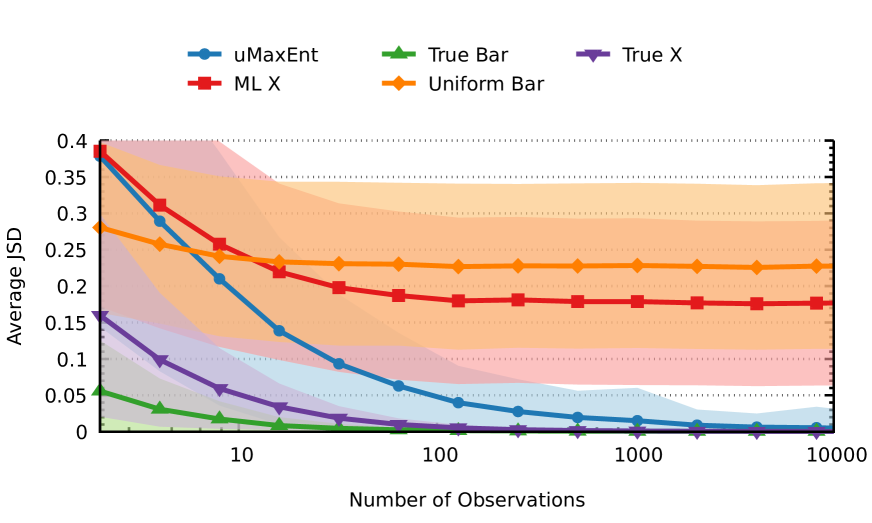
Figure 1: Average JSD achieved by various approaches in randomly generated programs. The colored area represents one standard deviation.

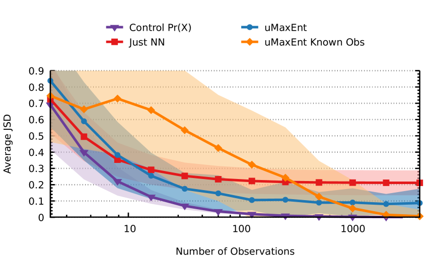
Figure 2: Average Total JSD achieved by various approaches in the color circles domain. The colored area represents one standard deviation.

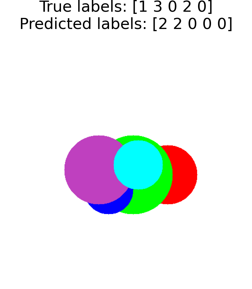
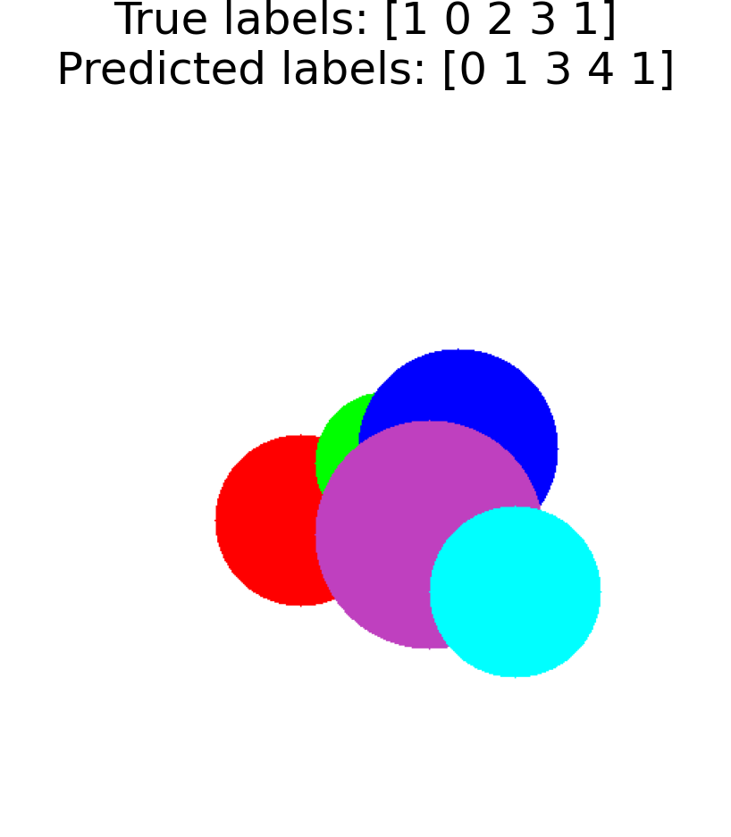
Figure 3: Two examples of images produced in the colored circles experiment. Left: True labels: [1 3 0 2 0] Predicted labels [2 2 0 0 0], Right: True labels [1 0 2 3 1], Predicted labels [0 1 3 4 1]

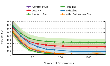
Figure 4: Average Total JSD achieved by various approaches in the color circles domain with regularization. Colored area represents one standard deviation.

4 Methods

4.1 Principle of Maximum Entropy Derivation

Suppose that we produce $N$ samples of $X\in\mathbb{X}$ from $Pr_{0}(X)$ and label the $i^{th}$ sample $X_{i}$. We may compute the resulting empirical distribution over $\mathbb{X}$ as $\tilde{Pr}(X)\triangleq{1\over N}\sum\limits_{i=0}^{N}\delta(X,X_{i})~{}\forall~{}X\in\mathbb{X}$, where $\delta$ is the Kronecker delta. In most cases, $N$ will be finite and therefore $\tilde{Pr}(X)$ is only expected to approximate $Pr_{0}(X)$ with the error approaching zero as $N\rightarrow\infty$ by the law of large numbers.

Besides $\tilde{Pr}(X)$ we may have extra information about the structure of $Pr_{0}(X)$ that we wish to incorporate into the posterior distribution $Pr(X)$. To this end, we define $K$ feature functions $\phi_{k}:X\Rightarrow\mathbb{R}$ that represent the relevant information we have about each $X$. We now require that our chosen distribution is constrained to match the expected features of the empirical distribution. Prior information may also be incorporated if available (See section 6.1).

The principle of maximum entropy with feature expectation constraints is expressed as the following convex non-linear program:

$$\max\left(-\sum\nolimits_{X\in\mathbb{X}}Pr(X)~{}log~{}Pr(X)\right)$$

subject to

$$\sum\nolimits_{X\in\mathbb{X}}Pr(X)=1$$

$$\sum\nolimits_{X\in\mathbb{X}}Pr(X)\phi_{k}(X)=\sum\nolimits_{X\in\mathbb{X}}\tilde{Pr}(X)\phi_{k}(X)~{}~{}~{}~{}~{}~{}\forall k$$ (3)

The feature expectation constraint may be written as $\Phi=\tilde{\Phi}$ for short.

The principle of maximum entropy as formulated in equation 3 has a number of well-known desirable properties. It is convex,${}^{\hbox{{\immediate{?}}}}$ ensuring that only one solution exists and improving the speed at which it can be solved. As entropy is the inverse of information${}^{\hbox{{\immediate{?}}}}$ choosing the one distribution with the maximum entropy ensures that the minimum amount of information is present in the solution: only that which is needed to satisfy the constraints. In other words, the information present in the feature expectations is encoded into $Pr(X)$ and no more, as any other information would necessarily reduce the entropy of $Pr(X)$ and a better solution to the program could be found. Importantly, we may therefore view the program as exactly encoding the feature expectations into one distribution over $\mathbb{X}$. Notice also that $Pr(X)$ could differ significantly from but will never have less entropy than $\tilde{Pr}(X)$.

To solve equation 3 and arrive at a closed form definition for $Pr(X)$, we begin by finding the Lagrangian relaxation of the program.

$$\mathcal{L}(Pr(X),\lambda,\eta)~{}=~{} -\sum\nolimits_{X\in\mathbb{X}}Pr(X)~{}log~{}Pr(X)+\eta\left(\sum\nolimits_{X\in\mathbb{X}}Pr(X)-1\right)+$$

$$\sum\limits_{k=1}^{K}\lambda_{k}\left(\sum\limits_{X\in\mathbb{X}}Pr(X)\phi_{k}(X)-\sum\limits_{X\in\mathbb{X}}\tilde{Pr}(X)~{}\phi_{k}(X)\right)$$ (4)

Since the program is convex, the Lagrangian function must be as well .${}^{\hbox{{\immediate{?}}}}$ Therefore, when the Lagrangian’s gradient is 0 we have found the global maximum. We now can find the definition of $Pr(X)$:

$${\partial\mathcal{L}(Pr(X),\lambda,\eta)\over\partial Pr(X)} ~{}=~{}-logPr(X)-1+\eta+\sum\limits_{k=1}^{K}\lambda_{k}\phi_{k}(X)$$

$$0 ~{}=~{}-logPr(X)-1+\eta+\sum\limits_{k=1}^{K}\lambda_{k}\phi_{k}(X)$$

$$Pr(X) ~{}=~{}{e^{\sum\limits_{k=1}^{K}\lambda_{k}\phi_{k}(X)}\over Z(\lambda)}$$ (5)

Where $Z(\lambda)~{}=~{}{(e^{-1}e^{\eta})}^{-1}~{}=~{}\sum\limits_{X^{\prime}\in\mathbb{X}}e^{\sum\limits_{k=1}^{K}\lambda_{k}\phi_{k}(X^{\prime})}$. Plugging our definition of $Pr(X)$ back into the Lagrangian, we arrive at the dual.

$$\mathcal{L}_{dual}(\lambda)~{}=~{}log~{}Z(\lambda)-\sum\limits_{k=1}^{K}\lambda_{k}\sum\limits_{X\in\mathbb{X}}\tilde{Pr}(X)\phi_{k}(X)$$ (6)

The dual may now be minimized by any convex optimization technique with gradient descent used in our work.

4.1.1 Noisy data

In the event that $X$ may only be partially observed, for instance if observations of $X$ are corrupted by noise, it is possible for standard maximum entropy approaches to fail as the empirical feature expectations could be unmatched with any distribution over $X$. However, in many problem domains noise is pervasive and not extreme and so we still wish to make use of the principle of maximum entropy to some degree.

In specific cases, it is possible to relax the feature expectation constraint to account for the observation error provided that the error is well characterized. Suppose for instance that the error is zero mean Gaussian. In this case, as the number of samples increases the error in the empirical features reduces to zero due to the law of large numbers. Then we may therefore relax the feature expectation constraint to account for the error as $\chi^{2}={{|\Phi-\tilde{\Phi}|^{2}}/\sigma^{2}}$, where $\sigma$ is the standard deviation and $\chi^{2}$ is the chi-squared distribution. Unfortunately, while possibly producing reasonable solutions, due to the constraint relaxation we may no longer interpret $Pr(X)$ as encoding only the information in the feature expectations. Instead we may say that the solution is the distribution with the maximum entropy found within the error bounds, making interpretation ad-hoc.

In more general situations where the error is not exactly known or not zero-mean it is common to simply select the most likely $X$ given an observation $\omega$, ie. $ML_{X}=\mathop{\mathrm{argmax}}\limits_{X}Pr(X|\omega)$. Knowing this method will be used, it is common practice to limit $\Omega$ to only those observations that exhibit this quality. However, there are serious concerns with this approach. As $Pr(X|\omega)\propto Pr(\omega|X)Pr(X)$, what should we choose $Pr(X)$ to be? Furthermore, if $Pr(\omega|X)$ is unknown the amount of error introduced into the posterior is also unknown. That said, for low entropy observations in which the most likely $X$ has a significant portion of the probability mass of $Pr(X|\omega)$, the error tends to be tolerable which explains the popularity of this method particularly in discrete $\mathbb{X}$ domains. Regardless, we cannot expect this approach to accurately encode the information available in the observations, even as the number of samples becomes very large.

Another limitation of this most-likely-$X$ approach is more subtle; all of the elements of $\mathbb{X}$ may not have observations of equal quality, leading to one or more $X$ that contribute much more error to the posterior than others. Faced with this situation, we have a number of unsatisfactory options. This error could be ignored, potentially throwing off results for other well observed elements, the problem observations could be removed and ad-hoc extrapolation techniques used to extend the learned distribution to those un-observed elements, or the problem elements could be removed entirely from the model. These solutions interfere with interpretation and reproducibility, as they introduce potentially significant effects on the model or posterior based upon the particular observation methods in use.

4.2 Principle of Uncertain Maximum Entropy Derivation

4.2.1 Unknown $\overline{Pr(X)}$

Given $N=\infty$ samples, $\tilde{Pr}(\omega)=Pr_{0}(\omega)$ and:

$$Pr_{0}(X) ~{}=~{}\sum\limits_{\omega\in\Omega}Pr_{0}(\omega)Pr(X|\omega)~{}~{}\forall~{}X$$

$$Pr_{0}(X) ~{}=~{}\sum\limits_{\omega\in\Omega}Pr_{0}(\omega){{Pr(\omega|X)}\overline{Pr(X)}\over\overline{Pr(\omega)}}~{}~{}\forall~{}X$$ (7)

But if we choose a uniform distribution for $\overline{Pr(X)}$ then:

$$Pr_{0}(X) ~{}\neq~{}\sum\limits_{\omega\in\Omega}Pr_{0}(\omega){1\over|\mathbb{X}|}{{Pr(\omega|X)}\over{\sum\limits_{X^{\prime}\in\mathbb{X}}{1\over|\mathbb{X}|}Pr(\omega|X^{\prime})}}$$

$$~{}=~{}\sum\limits_{\omega\in\Omega}\sum\limits_{X^{\prime\prime}\in\mathbb{X}}Pr(\omega|X^{\prime\prime})Pr_{0}(X^{\prime\prime}){{Pr(\omega|X)}\over{\sum\limits_{X^{\prime}\in\mathbb{X}}Pr(\omega|X^{\prime})}}$$ (8)

In fact, it is straightforward to see that there is only one possible value for $\overline{Pr(X)}$ that satisfies equation 7, $Pr_{0}(X)$. Of course, in the event the true distribution is uniform equation 8 is in fact correct.

4.2.2 Proof of uniqueness

To show that the principle of uncertain maximum entropy specifies a unique solution we must show that for any observation function used, which may not provide a way of distinguishing between different $X$ in certain cases, any local maxima solution found must be the global one. Our proof is based upon one found in .${}^{\hbox{{\immediate{?}}}}$

Theorem 1.

There exists only one distribution in the set of all $Pr(X)$ which can exactly satisfy the constraints in equation 1 and have the maximum entropy.

Proof.

Suppose that we are given $\tilde{Pr}(\omega)$ and $Pr(\omega|X)$. Assume that two $Pr(X)$ labeled $Pr_{b}(X)$ and $Pr_{c}(X)$ satisfy the constraints in equation 1 and have the maximum entropy. Let $Pr_{\alpha}(X)$ be an interpolation of $Pr_{b}(X)$ and $Pr_{c}(X)$ so that $Pr_{\alpha}(X)=(1-\alpha)Pr_{b}(X)+\alpha Pr_{c}(X)$, where $0\leq\alpha\leq 1$.

Since they are satisfying solutions, $\tilde{Pr}(\omega)=\sum\limits_{X\in\mathbb{X}}Pr(\omega|X)Pr_{b}(X)=\sum\limits_{X\in\mathbb{X}}Pr(\omega|X)Pr_{c}(X)$ for all $\omega$. Then $Pr_{\alpha}(X)$ also satisfies the constraints:

$$\sum\limits_{X\in\mathbb{X}}Pr(\omega|X)Pr_{\alpha}(X) =\sum\limits_{X\in\mathbb{X}}Pr(\omega|X)((1-\alpha)Pr_{b}(X)+\alpha Pr_{c}(X))$$

$$=(1-\alpha)\sum\limits_{X\in\mathbb{X}}Pr(\omega|X)Pr_{b}(X)+\alpha\sum\limits_{X\in\mathbb{X}}Pr(\omega|X)Pr_{c}(X)$$

$$=(1-\alpha)\tilde{Pr}(\omega)+\alpha\tilde{Pr}(\omega)$$

$$=\tilde{Pr}(\omega)$$

Now define the entropy of $Pr_{\alpha}(X)$ as a function of $\alpha$, $H(\alpha)$, where $H(0)=H(Pr_{b}(X))$ and $H(1)=H(Pr_{c}(X))$.

$$H(\alpha) =H((1-\alpha)Pr_{b}(X)+\alpha Pr_{c}(X))$$

$${d^{2}\over d\alpha^{2}}H(\alpha) ={d^{2}\over d\alpha^{2}}H((1-\alpha)Pr_{b}(X)+\alpha Pr_{c}(X))(-Pr_{b}(X)+Pr_{c}(X))^{2}$$

$$={d^{2}\over d\alpha^{2}}H(Pr_{\alpha}(X))(-Pr_{b}(X)+Pr_{c}(X))^{2}$$

As entropy is a convex function, ${d^{2}\over d\alpha^{2}}H(Pr_{\alpha}(X))<0$. So if $Pr_{b}(X)\neq Pr_{c}(X)$ then $H(\alpha)$ is a convex function in $\alpha$ as ${d^{2}\over d\alpha^{2}}H(\alpha)<0$. But then at least one of $Pr_{b}(X)$ and $Pr_{c}(X)$ cannot be the maximal point. Therefore we conclude that $Pr_{b}(X)=Pr_{c}(X)$. ∎

In other words, if the observations do not uniquely distinguish between different $X$, the principle of uncertain maximum entropy chooses the most uniform solution possible that matches the empirical observations. In the extreme, the observation function could provide no information about $Pr_{0}(X)$ at all.

Corollary 1.1.

If, for each $\omega$, $Pr(\omega|X)$ is equal for all $X$ the distribution over $\mathbb{X}$ chosen by the principle of uncertain maximum entropy is uniform.

4.2.3 Generalization of the Principle of Maximum Entropy

By contrast, if each observation could only be sampled given exactly one $X$, the principle of uncertain maximum entropy reduces to the standard principle of maximum entropy.

Theorem 2.

The principle of maximum entropy is a special case of the principle of uncertain maximum entropy in which for each $\omega$, $Pr(\omega|X)$ is non-zero for exactly one $X$ and for all $X$ at least one $Pr(\omega|X)$ is non-zero.

Proof.

Assume that for each $\omega$ the observation function $Pr(\omega|X)$ is non-zero for exactly one $X$. Then for any $Pr(X)$, $~{}Pr(X|\omega)=1~{}$if$~{}Pr(\omega|X)>0$; otherwise it must be 0. Thus $\sum\limits_{\omega\in\Omega}\tilde{Pr}(\omega)Pr(X|\omega)=\tilde{Pr}(X)$ for a given $X$. Therefore, for the constraint in equation 1 we have:

$$\sum\limits_{X\in\mathbb{X}}Pr(X)\phi_{k}(X) =\sum\limits_{\omega\in\Omega}\tilde{Pr}(\omega)\sum\limits_{X\in\mathbb{X}}Pr(X|\omega)~{}\phi_{k}(X)~{}~{}~{}\forall k$$

$$=\sum\limits_{X\in\mathbb{X}}~{}\phi_{k}(X)\sum\limits_{\omega\in\Omega}\tilde{Pr}(\omega)Pr(X|\omega)~{}~{}~{}\forall k$$

$$=\sum\limits_{X\in\mathbb{X}}\phi_{k}(X)~{}\tilde{Pr}(X)~{}~{}~{}\forall k$$

which is identical to that of equation 3 provided that for every $X$ at least one $Pr(\omega|X)$ is non-zero. ∎

4.2.4 Approximation and Expectation Maximization Solution

Because equation 1 is non-convex, we can not arrive at a closed-form definition for $Pr(X)$ using the zero point of its Lagrangian’s gradient. We will therefore approximate $Pr(X)$ to be log-linear and employ expectation-maximization to find solutions to the resulting Lagrangian function.

To start we take the Lagrangian.

$$\mathcal{L}^{U}(Pr(X),\lambda,\eta)~{}=~{} -\sum\limits_{X\in\mathbb{X}}Pr(X)~{}log~{}Pr(X)+\eta\left(\sum\nolimits_{X\in\mathbb{X}}Pr(X)-1\right)+$$

$$\sum\limits_{k=1}^{K}\lambda_{k}\left(\sum\limits_{X\in\mathbb{X}}Pr(X)\phi_{k}(X)-\sum\limits_{\omega\in\Omega}\tilde{Pr}(\omega)\sum\limits_{X}Pr(X|\omega)~{}\phi_{k}(X)\right)$$ (9)

And the Lagrangian’s gradient.

$${\partial\mathcal{L}^{U}(Pr(X),\lambda,\eta)}\over{\partial Pr(X)} ~{}=~{}-logPr(X)-1+\eta~{}+$$

$$\sum\limits_{k=1}^{K}\lambda_{k}\left(\phi_{k}(X)-\sum\limits_{\omega\in\Omega}\tilde{Pr}(\omega)\left(\phi_{k}(X){{Pr(\omega|X)Pr(\omega)-Pr(\omega|X)^{2}Pr(X)}\over{Pr(\omega)^{2}}}\right)\right)$$

$$~{}=~{}-logPr(X)-1+\eta+\sum\limits_{k=1}^{K}\lambda_{k}\phi_{k}(X)$$

$$-\sum\limits_{k=1}^{K}\lambda_{k}\sum\limits_{\omega\in\Omega}\tilde{Pr}(\omega)\left(\phi_{k}(X){{Pr(\omega|X)Pr(\omega)-Pr(\omega|X)^{2}Pr(X)}\over{Pr(\omega)^{2}}}\right)$$ (10)

Unfortunately, the existence of $Pr(X|\omega)$ on the right side of the constraints causes the derivative to be non-linear in $Pr(X)$. This is caused by equation 1 no longer being convex when $\overline{Pr(X)}=Pr(X)$.

To make further progress, we require a reasonable closed form approximation for $Pr(X)$. To arrive at one, we must make an assumption about the relationship between the model and observations, as we desire a definition of $Pr(X)$ that is independent of the methods used to observe it. In other words, every $X$ exists independently of the methods used to observe them and $\Omega$ is chosen such that $Pr_{0}(X)$ is not significantly altered by any of the observations in use. Given this, we drop the last term of equation 10 in order to approximate $Pr(X)$ to be log-linear in its features alone:

$${\partial\mathcal{L}^{U}(Pr(X),\lambda,\eta)}\over{\partial Pr(X)} ~{}\approx~{}-logPr(X)-1+\eta+\sum\limits_{k=1}^{K}\lambda_{k}\phi_{k}(X)$$

$$0 ~{}\approx~{}-logPr(X)-1+\eta+\sum\limits_{k=1}^{K}\lambda_{k}\phi_{k}(X)$$

$$Pr(X) ~{}\approx~{}{e^{\sum\limits_{k=1}^{K}\lambda_{k}\phi_{k}(X)}\over{Z(\lambda)}}$$ (11)

Now if we plug our approximation back into the Lagrangian we arrive at a function that appears similar to a Lagrangian dual:

$$\mathcal{L}_{psuedo-dual}^{U}(\lambda)~{}=~{}log~{}Z(\lambda)-\sum\limits_{k=1}^{K}\lambda_{k}\sum\limits_{\omega\in\Omega}\tilde{Pr}(\omega)\sum\limits_{X\in\mathbb{X}}Pr(X|\omega)\phi_{k}(X)$$ (12)

However, this function’s maxima is not located at a $\lambda$ that produces the correct $Pr(X)$ (this may be seen by noting its gradient is not zero when the constraints of equation 1 are satisfied). Therefore, unable to simply minimize this function directly, we take a different approach.

We will instead maximize the likelihood of the data using the well known expectation-maximization algorithm. In the below derivation we use subscripts to indicate that a distribution is parameterized with the respective variable. Particularly $\lambda^{\prime}$ is used to indicate the previous EM iteration’s $\lambda$ during expectation-maximization. The log likelihood of the observations is:

$$L(\lambda)~{}=~{} \sum\limits_{\omega\in\Omega}\tilde{Pr}(\omega)~{}\log~{}Pr(\omega)$$

$$~{}=~{} \sum\limits_{\omega\in\Omega}\tilde{Pr}(\omega)~{}\log~{}\sum\limits_{X\in\mathbb{X}}Pr_{\lambda}(\omega,X)$$

$$~{}=~{} \sum\limits_{\omega\in\Omega}\tilde{Pr}(\omega)~{}\log~{}\sum\limits_{X\in\mathbb{X}}\frac{Pr_{\lambda}(\omega,X)}{Pr_{\lambda^{\prime}}(X|\omega)}Pr_{\lambda^{\prime}}(X|\omega)$$

$$~{}\geq~{} \sum\limits_{\omega\in\Omega}\tilde{Pr}(\omega)\sum\limits_{X\in\mathbb{X}}Pr_{\lambda^{\prime}}(X|\omega)\log\frac{Pr_{\lambda}(\omega,X)}{Pr_{\lambda^{\prime}}(X|\omega)}$$

$$~{}=~{} \sum\limits_{\omega\in\Omega}\tilde{Pr}(\omega)\sum\limits_{X\in\mathbb{X}}Pr_{\lambda^{\prime}}(X|\omega)\log Pr_{\lambda}(\omega,X)-\sum\limits_{\omega\in\Omega}\tilde{Pr}(\omega)\sum\limits_{X\in\mathbb{X}}Pr_{\lambda^{\prime}}(X|\omega)\log Pr_{\lambda^{\prime}}(X|\omega)$$

$$~{}=~{} \sum\limits_{\omega\in\Omega}\tilde{Pr}(\omega)\sum\limits_{X\in\mathbb{X}}Pr_{\lambda^{\prime}}(X|\omega)\log\left(Pr_{\lambda}(\omega|X)Pr_{\lambda}(X)\right)+H^{X}(\lambda^{\prime})$$

$$~{}=~{} \sum\limits_{\omega\in\Omega}\tilde{Pr}(\omega)\sum\limits_{X\in\mathbb{X}}Pr_{\lambda^{\prime}}(X|\omega)\log Pr_{\lambda}(X)+\sum\limits_{\omega\in\Omega}\tilde{Pr}(\omega)\sum\limits_{X\in\mathbb{X}}Pr_{\lambda^{\prime}}(X|\omega)\log Pr_{\lambda}(\omega|X)$$

$$+H^{X}(\lambda^{\prime})$$

$$~{}=~{} Q(\lambda,\lambda^{\prime})+\sum\limits_{\omega\in\Omega}\tilde{Pr}(\omega)\sum\limits_{X\in\mathbb{X}}Pr_{\lambda^{\prime}}(X|\omega)\log Pr_{\lambda}(\omega|X)+H^{X}(\lambda^{\prime})$$

$$~{}=~{} Q(\lambda,\lambda^{\prime})+\sum\limits_{\omega\in\Omega}\tilde{Pr}(\omega)\sum\limits_{X\in\mathbb{X}}Pr_{\lambda^{\prime}}(X|\omega)\log Pr(\omega|X)+H^{X}(\lambda^{\prime})$$ (13)

$$~{}=~{} Q(\lambda,\lambda^{\prime})+H^{\omega}(\lambda^{\prime})+H^{X}(\lambda^{\prime}).$$ (14)

Equation 13 follows because we assume the observation function $Pr(\omega|X)$ is known and does not depend on $\lambda$. This leaves $Q(\lambda,\lambda^{\prime})$ as the only function which depends on $\lambda$. For the sake of completeness, we note that $H^{X}(\lambda^{\prime})$ the empirical conditional entropy of the model and $H^{\omega}(\lambda^{\prime})$ is the conditional entropy of the observation function if $\tilde{Pr}(\omega)=Pr_{\lambda^{\prime}}(\omega)$. While these impact the data likelihood they do not alter the solution as they do not depend upon $\lambda$.

We now substitute the log-linear model of $Pr(X)$ (Eq. 11) into $Q(\lambda,\lambda^{\prime})$:

$$Q(\lambda,\lambda^{\prime}) ~{}=~{}\sum\limits_{\omega\in\Omega}\tilde{Pr}(\omega)\sum\limits_{X\in\mathbb{X}}Pr_{\lambda^{\prime}}(X|\omega)~{}\log Pr_{\lambda}(X)$$

$$~{}=~{}\sum\limits_{\omega\in\Omega}\tilde{Pr}(\omega)\sum\limits_{X\in\mathbb{X}}Pr_{\lambda^{\prime}}(X|\omega)\left(\sum\limits_{k=1}^{K}\lambda_{k}\phi_{k}(X)-~{}\log Z(\lambda)\right)$$

$$~{}=~{}-\log Z(\lambda)+\sum\limits_{k=1}^{K}\lambda_{k}\sum\limits_{\omega\in\Omega}\tilde{Pr}(\omega)\sum\limits_{X\in\mathbb{X}}Pr_{\lambda^{\prime}}(X|\omega)\phi_{k}(X).$$ (15)

The expectation-maximization algorithm proceeds by iteratively maximizing $Q$, and upon convergence $\lambda=\lambda^{\prime}$, at which point the likelihood of the data is at a stationary point (first derivative is zero). EM is guaranteed to converge to such points as the likelihood monotonically increases each iteration .${}^{\hbox{{\immediate{?}}}}$

Notice that at convergence, when $\lambda=\lambda^{\prime}$, equation 15 is the exact negative of equation 12. It remains to be shown, however, that all stationary points that equation 15 may converge to satisfy the constraints of equation 1.

Theorem 3.

If expectation-maximization has converged on a point where $\lambda=\lambda^{\prime}$, then $Pr(X)$ computed using equation 11 satisfies the feature expectation constraints of equation 1.

Proof.

As EM converges on zero-points of the gradient of $L(\lambda)$, we first find the gradient of the data likelihood with respect to each element of $\lambda$ assuming a log-linear $Pr(X)$.

$${d\over d\lambda_{i}} L(\lambda)=\sum\limits_{\omega\in\Omega}{\tilde{Pr}(\omega)\over Pr_{\lambda}(\omega)}{d\over d\lambda_{i}}Pr_{\lambda}(\omega)$$

$$=\sum\limits_{\omega\in\Omega}{\tilde{Pr}(\omega)\over Pr_{\lambda}(\omega)}\sum\limits_{X\in\mathbb{X}}Pr(\omega|X)\left(-({\sum\limits_{X^{\prime}\in X}\phi_{i}(X^{\prime})e^{\sum\limits_{k}\lambda_{k}\phi_{k}(X^{\prime})}\over Z(\lambda)^{2}}e^{\sum\limits_{k}\lambda_{k}\phi_{k}(X)})+{\phi_{i}(X)e^{\sum\limits_{k}\lambda_{k}\phi_{k}(X)}\over Z(\lambda)}\right)$$

$$=\sum\limits_{\omega\in\Omega}{\tilde{Pr}(\omega)\over Pr_{\lambda}(\omega)}\sum\limits_{X\in\mathbb{X}}Pr(\omega|X)\left(-(Pr_{\lambda}(X)\sum\limits_{X^{\prime}\in X}\phi_{i}(X^{\prime})Pr_{\lambda}(X^{\prime}))+\phi_{i}(X)Pr_{\lambda}(X)\right)$$

$$=-\sum\limits_{\omega\in\Omega}\tilde{Pr}(\omega)\sum\limits_{X\in\mathbb{X}}Pr(X|\omega)\sum\limits_{X^{\prime}\in X}Pr_{\lambda}(X^{\prime})\phi_{i}(X^{\prime})+\sum\limits_{\omega\in\Omega}\tilde{Pr}(\omega)\sum\limits_{X\in\mathbb{X}}Pr_{\lambda}(X|\omega)\phi_{i}(X)$$

$$=-\sum\limits_{X^{\prime}\in X}Pr_{\lambda}(X^{\prime})\phi_{i}(X^{\prime})\sum\limits_{\omega\in\Omega}\tilde{Pr}(\omega)\sum\limits_{X\in\mathbb{X}}Pr(X|\omega)+\sum\limits_{\omega\in\Omega}\tilde{Pr}(\omega)\sum\limits_{X\in\mathbb{X}}Pr_{\lambda}(X|\omega)\phi_{i}(X)$$

$$=-\sum\limits_{X\in X}Pr_{\lambda}(X)\phi_{i}(X)+\sum\limits_{\omega\in\Omega}\tilde{Pr}(\omega)\sum\limits_{X\in\mathbb{X}}Pr_{\lambda}(X|\omega)\phi_{i}(X)$$

As can be seen, the gradient of the observation data’s log likelihood is identical to the feature expectation constraints of equation 1. All stationary points, where ${d\over d\lambda_{i}}L(\lambda)=0$, therefore occur whenever the constraints of equation 1 are satisfied. ∎

Therefore, a stationary point arrived at by EM will provide one potential solution to the principle of uncertain maximum entropy with log-linear approximation. Working backwards, the process of maximizing $Q(\lambda,\lambda^{\prime})$ is equivalent to solving the following convex program by minimizing its Lagrangian dual, where we abuse notation slightly to mark the respective parameterization of $Pr(X)$:

$$\max~{}\left(-\sum\nolimits_{X\in\mathbb{X}}Pr_{\lambda}(X)~{}\log~{}Pr_{\lambda}(X)\right)$$

subject to

$$\sum\nolimits_{X\in\mathbb{X}}Pr_{\lambda}(X)=1$$

$$\sum\limits_{X\in\mathbb{X}}Pr_{\lambda}(X)\phi_{k}(X)=\sum\limits_{\omega\in\Omega}\tilde{Pr}(\omega)\sum\limits_{X\in\mathbb{X}}Pr_{\lambda^{\prime}}(X|\omega)~{}\phi_{k}(X)~{}~{}~{}\forall k$$ (16)

which exactly equals Eq. 1 at EM convergence. Therefore, we have found a convex approximation to the principle of uncertain maximum entropy.

However, as EM is well known to become trapped in local maxima, restarts with different initial $\lambda^{\prime}$ are recommended. The solution found with the maximum entropy can then be chosen. Thus, we arrive at algorithm 1.

4.3 Experimental Details

4.3.1 Comparative Performance on Random Models

Program Generation

This experiment was run in a block structure, with an equal number of data points for each configuration (barring errors). $|\mathbb{X}|$ is fixed at 10, while $|\Omega|$ may vary between 10, 20, 50, 100, 150, 200, 300. $Pr_{0}(X)\propto e^{\alpha*U(-1,1)}$, where $\alpha$ varies between 1, 2, 3, 4, 5 and $U$ is the uniform distribution.

To generate $Pr(\omega|X)$, we must choose only those distributions that are compatible with the most-likely-X control. Specifically, each $X$ must have at least one $\omega$ such that $X=arg~{}maxPr(X|\omega)$, otherwise, one or more $X$ could never be observed. We achieve this in two steps:

1. Generate all $Pr(\omega|X)\propto e^{\beta*U(0,1)}$ where $\beta$ varies between 1, 2, 3, 4, 5

2. For each $X$, choose one $\omega$ and add $1.0/|\Omega|$ to $Pr(\omega|X)$, then re-normalize.

This process was repeated until a usable observation function was generated.

The feature functions $\phi_{k}(X)$ were chosen to be uninformative, for each experiment $K=|X|$ and the $i^{th}$ feature returned 1.0 for $X_{i}$ and 0 for all others.

Solvers

To solve the M step of uMaxEnt, we make use of gradient descent to minimize equation 12’s gradient. Specifically, we use unconstrained adaptive exponentiated gradient descent ${}^{\hbox{{\immediate{?}}}}$ with path length bounds. We additionally split the weights into positive and negative components to allow $\lambda$ to range from $[-\infty,\infty]$ as in .${}^{\hbox{{\immediate{?}}}}$

There are 3 conditions under which gradient descent stops:

1. The maximum number of iterations could be reached, here set to 5000

2. The L2 norm of $\lambda$ could exceed a limit, here set to 50

3. The standard deviation of the error of the last 5 iterations could fall below a tolerance, indicating convergence. Here the tolerance is set to 0.0000001, and error is calculated as the L1 norm of gradient $+i$ for the $i^{th}$ term to avoid a corner case where components could swap error values on subsequent iterations yet appear to have 0 standard deviation.

At solving start the learning rate for gradient descent is set to 1, each iteration we add 0.00001 to the learning rate to increase the rate of convergence. If the learning rate is too high, oscillation may occur due to over-shooting. Oscillation is detected by comparing the weights of the last five iterations component-wise and marking increases and decreases. If more than 3 switches between a weight increasing and decreasing are found then an oscillation is declared, and the learning rate is multiplied by 0.99.

Expectation-Maximization is continued for a maximum of 5000 iterations, and was stopped early if the L2 Norm of the difference between subsequent $\lambda$ is less than 0.001 or the L2 Norm of the latest $\lambda$ is greater than 50. Each iteration, the last learning rate for gradient descent is multiplied by 1.1 and the next M step uses the increased rate, this is capped at 1000. Initial $\lambda^{\prime}$ were chosen uniformly from $[-0.01,0.01]$ component-wise.

Procedure

Each configuration of parameters was repeated over 1000 times, with each repeat proceeding as follows:

1. Generate $Pr_{0}(X)$ and $Pr(\omega|X)$ as above

2. Sample from $Pr_{0}(X)$, $2^{18}$ times

3. For each $X$ sample, sample once from $Pr(\omega|X)$

4. Repeat for observations $[1,2^{[0,18]}]$:

   1. Generate initial $\lambda^{\prime}$

   2. Use the initial $\lambda^{\prime}$ to compute $Pr(X)$. This provides an uninformative prior or initial E Step $Pr(X)$, depending upon the algorithm in use.

   3. Solve each algorithm variant

   4. Record metrics

4.3.2 Image Recognition Domain

4.3.3 Neural Networks and Deep Learning

The following background provides an overview of Neural networks, their development into deep neural network models, and a focus on training a variant of deep neural networks, namely a convolutional neural network, for use as a discriminative model in our experiments with supervised learning.

Neural networks consist of connections between individual computational units called Artificial neurons $a$, or simply neurons. in which a specific neuron $a_{i}$ processes input $\omega$ and gives a prediction $\hat{X}$. An individual neuron $a_{i}^{j}$ maintains its connections through a directed link consisting of weights $\bm{w}$ and biases $\bm{b}$ known as parameters $\theta$. These $a_{\theta}$ in conjunction with nonlinear operations, known as their activation functions, produce a neurons output $a_{i}^{J}=\hat{X}$ which forwardly propagates information throughout the network. Groups of similar neurons $\sum_{j=1}^{N-1}a^{j}$ are stacked into layers, where $N$ represents the total amount of layers in a network. It is by repeatedly stacking layers between the input and output layers, we obtain a deep learning network and as such are able to model more intricate functions from increasingly complex data, as can be seen in fig. LABEL:fig:deepnet.

In our experiments we train a popular variant of Deep Neural Network (DNN) known as a Convolutional Neural Network through the supervised learning method of feedback as follows. Let us take observations $\omega\in\Omega$ such that our discriminative a model learns a function over similar a similar space $X\in\mathbb{X}$. Therefore, we obtain dataset $\Omega$ as generated from the ground truth set $\mathbb{X}$. Our dataset contains images of dimension $RxC$ to obtain $N$ number of samples $\omega$ with corresponding labels $X$. The task given to our model is provided there exists some unknown function we wish to learn $\mathcal{F}(\omega)=X$ approximate such function with $\mathcal{F}^{*}(\omega)=\hat{X}$ such that $X=\hat{X}$. Similarly, we may look at this model as learning parameters $\theta$ taken from total features $\bm{{\phi}}\in\phi(\omega)$ such that it learns the distribution $y=\mathcal{F}(\omega;\bm{\theta},\bm{w})=\phi(\omega;\bm{\theta})^{\top}\bm{w}$.

In order to learn such a distribution our CNN extracts such $\phi$ through a series of sequential Convolutional-Pooling operations. For a Convolution layer, it does so through the use of multiple kernels. Whereby it creates a feature map from input vector $\omega=RxC$ to produce output size $(R-r+1)\times(C-c+1)$ fig. LABEL:fig:featuremap.

Note this is done per RGB dimension, each Conv2D output is passed through our non-linear activation function ReLU, $Relu(z)=max(0,z)$, which has become standard. $z$ arrives at a Pooling layer which gives the max value for a specified neighborhood in each matrix grid $Z_{pool}(k,i,j)=\max_{l\in[i,i+s],m\in[j,j+s]}Z(k,l,m)$.

After such Convolutional-Pooling operations the output is then flattened to be classified by densely connected layers as depicted in the aforementioned figure. Given an input $\omega$, the neurons at dense layer $a^{i}$ compute output $z$, such that

$$\sigma(\bm{z})=\bm{w}^{\top}\omega+b=b+\sum_{i=1}^{m}\alpha_{ij}\omega^{\top}$$

Where $\bm{\theta}=\bm{w},b$. This output completes the forward feed which will be used with Stochastic Gradient Descent with Adam optimizer, to give our per-example objective function to minimize during backpropagation.

$$J(\bm{\theta})=\mathbb{E}_{\omega,X\sim\hat{p}_{\mathrm{data}}}L_{CE}(\omega,X,\bm{\theta})=\frac{1}{m}\sum_{i=1}^{m}L_{CE}\left(\omega^{(i)},X^{(i)},\bm{\theta}\right)$$ (17)

$$\nabla_{\theta}J(\bm{\theta})=\frac{1}{m}\sum_{i=1}^{m}\nabla_{\theta}L_{CE}\left(\omega^{(i)},X^{(i)},\bm{\theta}\right)$$ (18)

The gradients computed from the resultant equation will be used to update our parameters $\theta$ for the Network in order to achieve best fitting $\mathcal{F^{*}}$. We now iterate over the training data set in batches in order to attempt to increase the accuracy of the model.

Given that we only need to produce some prediction accuracy our Convolution Neural Network (CNN) will extract relevant features $\phi$ but also, provide adequate dimensionality reduction while attempting to minimize the inherent information loss. To produce $Pr(\hat{X}|X)$ where X is an observation in similar space $\Omega$, our CNN computes and outputs the probability given the Softmax function:

$$\sigma(z_{i})=\frac{e^{z_{i}}}{\sum_{j=1}^{K}e^{z_{j}}}\ \ \ for\ i=1,2,\dots,\mathcal{C}$$

Where we take $\mathcal{C}$ to be the number of class labels. This output will be fed into a chosen loss function dependent on the label’s encoding i.e categorical, numeric, etc. Discriminitive supervised learning models use the encoded ground truth labels, contrasted against that of cross-entropy, to generate their specific loss function $L_{CE}=-\sum_{i=1}^{n}t_{i}\log\left(p_{i}\right)$. where $p_{i}$ is the probability output from Softmax. Such that the resultant accuracy is given by accuracy $Accuracy=\frac{TP+TN}{TP+TN+FP+FN}$ Where $TP$ is our True positive, $TN$ True negative, $FP$ False positive, $FN$ False negative respectively. This metric will allow us to view how effective current decision boundary is while updating model parameters $\theta$.

4.3.4 Experimental Setup

We use Tensorflow 2.11.0-gpu to implement our CNN model architecture. Additionally, The computer hardware used for training was Intel(R) Xeon(R) CPU @ 2.20GHz, 52G RAM, and 16G Tesla V100.

For our dataset we draw 5 colored circles on a 512x512 pixel image, one after another, the circles drawn earlier may be drawn over by the later ones. In our configuration, the color of the circles is unique, allowing identification of each one provided that it is visible.

The Colored Circles dataset was randomly generated using the PyOpenCV library where the (x,y) for each center of the five circles was drawn from a binomial distribution. We used this to produce images of size 512x512x3 RGB , using them 70-20-10 split for training, validation, and test size respectively. The architecture of our model is shown in table LABEL:tab:model_architecture.

Furthermore, to simplify implementation and neural network training, we exploit the independence between the individual circles in $X$ and transform the problem into estimating 5 distributions, one for each circle’s size, from a given image. Due to the independence we may calculate the probability of an image given one specific circle’s size as $Pr(\omega|X_{1})=\sum\limits_{X_{2},X_{3},X_{4},X_{5}}Pr(\omega|X_{1},X_{2},X_{3},X_{4},X_{5})=\sum\limits_{X_{2},X_{3},X_{4},X_{5}}Pr(\omega|X)$.

In our experiments we used categorical cross entropy to produce inference when given inputs $\omega$. Our CNN model will output a matrix 5x5 where each row is corresponding to a circle of a distinct color and each index will be according to one of five sizes. For example, the table LABEL:tab:output corresponds to an image in which the first vector of five is a blue circle, the next green, the next red,etc.

To generate $Pr(X^{\prime}|X)$, we produce 10,000 samples of $X$ from a uniform distribution and produce an image for each of them, then obtain the predictions of $X$ for each by the Neural Network. It is straightforward to then compute $Pr(X^{\prime}|X)$ as $X$ is known for each sample.

The feature functions $\phi_{k}(X)$ were chosen to be uninformative, for each experiment $K=5*|X_{i}|$ and the $j^{th}$ feature returned 1.0 for $X_{i,j}$ and 0 for all others.

Solvers

The M step is solved as with the smaller domain, with the only difference being the learning rate was initialized to 0.01. Expectation-Maximization is identical as well.

Procedure

This procedure was repeated 100 times for all configurations except uMaxEnt Known Obs.

1. Generate $Pr_{0}(X_{i})\propto e^{8*U(0,1)}$

2. Generate 65535 samples of $Pr_{0}(X)\propto\prod\limits_{i}^{5}Pr_{0}(X_{i})$

3. Generate one image for each sampled $X$

4. Provide image as input into the trained neural network, record its output

5. Repeat for image $[1,2^{[0,16]}]$:

   1. Generate initial $\lambda^{\prime}$

   2. Use the initial $\lambda^{\prime}$ to compute $Pr(X)$. This provides an uninformative prior or initial E Step $Pr(X)$, depending upon the algorithm in use.

   3. Solve each algorithm variant

   4. Record metrics, specifically we sum the JSD of the posterior distribution over each element of $X$ compared to the true distribution.

For uMaxEnt Known Obs, the large amount of time to generate $Pr(\omega|X)$ for all $X$ and each image meant that only 20 unique $Pr_{0}(X)$ were considered. We then extend this to 100 repeats by reusing each set of samples 5 times and randomizing the samples chosen within each repeat. Otherwise, the procedure continued as above.

$Pr(\omega|X)$ was computed by considering all possible positions that each circle could be in for a given image and $X$, then summing up the binomial distribution’s probability of each center position, for each possible $X$.

5 Data and Code Availability

The code for implementing uMaxEnt and corresponding image domain is publicly available via gitlab at: https://www.gitlab.cs.unca.edu/kbogert/umaxent

All code provided is listed under the MIT license which allows for free use, modification, and distribution.

Furthermore, the generated dataset with corresponding labels may be downloaded${}^{\hbox{{\immediate{?}}}}$

6 Supplementary Text

6.1 Use of Priors with the Principle of Maximum Entropy

The Principle of Maximum Entropy may be thought of as a special case of the Principle of Minimum Cross Entropy .${}^{\hbox{{\immediate{?},\penalty 1000\hskip 0.91003pt plus 0.70004pt minus 0.70004pt{?},\penalty 1000\hskip 0.91003pt plus 0.70004pt minus 0.70004pt{?}}}}$ Suppose that we have a prior distribution $q(X)$ whose information we wish to incorporate into $Pr(X)$ in addition to $\tilde{Pr}(X)$. The Principle of Minimum Cross Entropy specifies that we should choose the distribution that requires the least additional information from $q(X)$ while satisfying the constraints. In other words, in the set of all $Pr(X)$ that satisfy the constraints we should choose the one that is most similar to $q(X)$ as measured by the Kullback–Leibler divergence. Replace the objective in equation 3 with:

$$min~{}D_{KL}(Pr(X)~{}||~{}q(X)) ~{}=~{}\sum\limits_{X\in\mathbb{X}}Pr(X)~{}log~{}{Pr(X)\over q(X)}$$

$$~{}=~{}\sum\limits_{X\in\mathbb{X}}Pr(X)~{}log~{}Pr(X)-Pr(X)~{}log~{}q(X)$$

$$~{}=~{}I(Pr(X),~{}q(X))$$

Solving, we find the definition of $Pr(X)~{}=~{}q(X)e^{\sum\limits_{k=1}^{K}\lambda_{k}\phi_{k}(X)}/Z(\lambda)$, where
$Z(\lambda)~{}=~{}{(e^{-1}e^{\eta})}^{-1}~{}=~{}\sum\limits_{X^{\prime}\in\mathbb{X}}q(X)e^{\sum\limits_{k=1}^{K}\lambda_{k}\phi_{k}(X^{\prime})}$

In the event that $q(X)$ is the uniform distribution the Principle of Minimum Cross Entropy is equivalent to the Principle of Maximum Entropy.

6.2 Missing data

In some scenarios that we would wish to utilize the principle of maximum entropy some portion of $X$ is hidden from observation due to occlusion,${}^{\hbox{{\immediate{?}}}}$ underlying hidden structure, or missing data. Wang et al.${}^{\hbox{{\immediate{?}}}}$ model this as $X$ containing a latent variable and describe the principle of latent maximum entropy which generalizes standard MaxEnt to these scenarios.

Divide every $X$ into $Y$ and $Z$ such that $X=Y\cup Z$ and $Pr(X)~{}=~{}Pr(Y,Z)$. $Y$ is the portion of $X$ that is perfectly observed while $Z$ is perfectly hidden, and let $Z_{Y}$ be the set of every $Z$ which when combined with $Y$ forms a $X\in\mathbb{X}$ . Instead of empirically observing samples of $X$, we instead receive $N$ samples of $Y$ to compute an empirical distribution $\tilde{Pr}(Y)$. Latent maximum entropy is now defined as:

$$\max\left(-\sum\nolimits_{X\in\mathbb{X}}Pr(X)~{}log~{}Pr(X)\right)$$

subject to

$$\sum\nolimits_{X\in\mathbb{X}}Pr(X)=1$$

$$\sum\nolimits_{X\in\mathbb{X}}Pr(X)\phi_{k}(X)=\sum\limits_{Y\in\mathbb{Y}}\tilde{Pr}(Y)\sum\limits_{Z\in Z_{Y}}Pr(Z|Y)\phi_{k}(X)~{}~{}~{}~{}~{}~{}\forall k$$ (19)

Intuitively, this program corrects for the missing portion of $X$ in the empirical data by constraining the distribution over $X$ to match the feature expectations of the observed components $Y$ while taking into account any known structure in the hidden portion $Z$. Notice that $Pr(Z|Y)={Pr(X)\over\sum\nolimits_{X^{\prime}\in\mathbb{X}}Pr(X^{\prime})}$, therefore the right side of the constraint which computes the empirical feature expectations has a dependency on the program solution. In fact, the principle of latent maximum entropy is a special case of the principle of uncertain maximum entropy.

To see this, we first need to define $Pr(\omega|Y)$. If we assume that all $Z$ are perfectly hidden, they must have no effect on the observation function. In other words, $Pr(\omega|X)=Pr(\omega|Y,Z)=Pr(\omega|Y)$ for any $Z\in Z_{Y}$ and each $\omega$.

Theorem 4.

The principle of latent maximum entropy is a special case of the principle of uncertain maximum entropy in which for each $\omega$, $Pr(\omega|Y)$ is non-zero for exactly one $Y$ and for all $Y$ at least one $Pr(\omega|Y)$ is non-zero.

Proof.

Assume that $Z$ is perfectly hidden and the observation function $Pr(\omega|Y)$ is non-zero for exactly one $Y$. Then for any $Y$ and $\omega$ such that $Pr(\omega|Y)$ is non-zero,

$$Pr(X|\omega) ={Pr(\omega|X)Pr(X)\over Pr(\omega)}$$

$$={Pr(\omega|Y,Z)Pr(Y,Z)\over Pr(\omega)}$$

$$={Pr(\omega|Y)Pr(Z|Y)Pr(Y)\over\sum\limits_{Y^{\prime}\in Y}Pr(\omega|Y^{\prime})Pr(Y^{\prime})}$$

$$={Pr(\omega|Y)Pr(Z|Y)Pr(Y)\over Pr(\omega|Y)Pr(Y)}$$

$$=Pr(Z|Y)$$

otherwise $Pr(X|\omega)$ must be 0. Now define an indicator function $\delta(\omega,Y)$ which is 0 if $Pr(\omega|Y)=0$ and otherwise is 1. Thus $Pr(X|\omega)=Pr(Z|Y)\delta(\omega,Y)$ and $\sum\limits_{\omega\in\Omega}\tilde{Pr}(\omega)\delta(\omega,Y)=\tilde{Pr}(Y)={1\over N}\sum\limits_{i=0}^{N}\delta(Y,Y_{i})~{}\forall~{}Y$, where $\delta(Y,Y_{i})$ is the Kronecker delta.

For the constraint in equation 1 we now have:

$$\sum\limits_{X\in\mathbb{X}}Pr(X)\phi_{k}(X) =\sum\limits_{\omega\in\Omega}\tilde{Pr}(\omega)\sum\limits_{X\in\mathbb{X}}Pr(X|\omega)~{}\phi_{k}(X)~{}~{}~{}\forall k$$

$$=\sum\limits_{\omega\in\Omega}\tilde{Pr}(\omega)\sum\limits_{Y,Z\in\mathbb{X}}Pr(X|\omega)~{}\phi_{k}(X)~{}~{}~{}\forall k$$

$$=\sum\limits_{\omega\in\Omega}\tilde{Pr}(\omega)\sum\limits_{Y\in Y}\sum\limits_{Z\in Z_{Y}}Pr(Z|Y)\delta(\omega,Y)~{}\phi_{k}(X)~{}~{}~{}\forall k$$

$$=\sum\limits_{Y\in Y}\sum\limits_{Z\in Z_{Y}}~{}Pr(Z|Y)\phi_{k}(X)\sum\limits_{\omega\in\Omega}\tilde{Pr}(\omega)\delta(\omega,Y)~{}~{}~{}\forall k$$

$$=\sum\limits_{Y\in Y}\sum\limits_{Z\in Z_{Y}}~{}Pr(Z|Y)\phi_{k}(X)\tilde{Pr}(Y)~{}~{}~{}\forall k$$

$$=\sum\limits_{Y\in Y}\tilde{Pr}(Y)\sum\limits_{Z\in Z_{Y}}~{}Pr(Z|Y)\phi_{k}(X)~{}~{}~{}\forall k$$

which is identical to that of equation 19 provided that for every $Y$ at least one $Pr(\omega|Y)$ is non-zero. ∎

6.3 Most-Likely-$X$ Incompatible Observations

Due to the difficulty in obtaining $Pr(\omega|X)$ in many domains it has become common place to engineer $\Omega$ (and sometimes $\mathbb{X}$) to only consider observations that place a high probability mass on a single $X$, ie they have a low amount of error. Often, however, many more types of observations are available and, provided $Pr(\omega|X)$ may be adequately known, uMaxEnt may utilize them in addition to low error observations.

For example, suppose we have a set of negative observations, those that tell us with certainty which $X$ has not occurred. We may say that $Pr(\omega|X)$ is uniform except for $Pr(\omega_{i}|X_{i})$, which is zero. Clearly, these observations provide very little information as $|X|$ grows, and are not usable with the practice of selecting the most likely $X$ given $\omega$. However, as can be seen in figure 5, uMaxEnt still converges towards zero as the number of observations increases.

Interestingly, for larger $|X|$ the error, as measured by Jensen-Shannon divergence, increases until the number of observations reaches approximately $|X|$. We explain this by noting that, when these observations are in such low quantity, the $Pr(X)$ found is likely to be very incorrect. Consider the $Pr(X)$ for $N=1$ observation; whichever $X$ is contra-indicated by the observation received will be given lower probability and, due to the observations providing no other information, all other $X$ are given the same, higher probability. As more observations are received, $Pr(X)$ begins to become a (still incorrect) low-entropy distribution as these types of observations are well mixed, meaning most $X$ will likely have a negative observation. As $N$ becomes greater than $|X|$, this effect reduces and the error improves. Notice that the most likely $X$ approach converges on an extremely high error, which is approximately the error achieved by uMaxEnt at $N=2$, indicating that this method is converging on an approximately uniform $Pr(X)$. This is expected, as choosing the most likely $X$ given a negative observation is only slightly better than choosing $X$ at random.

Figure 5: Average JSD achieved using negative observations for uMaxEnt and a most-likely-$X$ approach. Size of $|X|$ as marked, with $|\Omega|$ matching.

7 Corresponding Author

Correspondence and requests for materials should be addressed to Kenneth Bogert (kbogert@unca.edu) .

8 Author Contributions

.

Kenneth Bogert was responsible for the overall concept, proofs, experiment design, software design and implementation of all components except those black-box related, data gathering and analysis, initial paper draft except black-box related sections, and review and editing of the paper.

Matthew Kothe provided the software design of black box and subsequent training, review and editing of paper, original writing of introduction and neural network sections.

All authors have read and agreed to the published version of the manuscript.”, please turn to the for the term explanation. Authorship must be limited to those who have contributed substantially to the work reported.

9 Competing Interests Declaration

The authors declare no conflict of interest.

References

- 1. E. T. Jaynes, Information theory and statistical mechanics. Physical Review, 106(4), 620 (1957).
- 2. M. Marsili, I. Mastromatteo, On the criticality of inferred models, Journal of Statistical Mechanics: Theory and Experiment, 10, P10012 (2011).
- 3. S. Singh, T. Joachims, A maximum entropy model for part-of-speech tagging, in Proceedings of the 2018 Conference on Empirical Methods in Natural Language Processing, (2018), pp. 390–399.
- 4. J. Elith, S. J. Phillips, T. Hastie, M. Dudík, Y. E. Chee, C. J. Yates, A statistical explanation of MaxEnt for ecologists, Diversity and Distributions, vol. 17, no. 1, 43–57 (2011).
- 5. S. Boyd, L. Vandenberghe, Convex Optimization. (Cambridge University press, 2004).
- 6. N. Wu, The maximum entropy method. (Springer Science & Business Media, 2012).
- 7. G. J. McLachlan, T. Krishnan, The EM algorithm and extensions. (John Wiley & Sons, 2007).
- 8. K. Bogert, and P. Doshi, A Hierarchical Bayesian Process for Inverse RL in Partially-Controlled Environments. in Proceedings of the 21st International Conference on Autonomous Agents and Multiagent Systems, (2022), pp. 145–153.
- 9. M. Baradad, V. Ye, A. B. Yedidia, F. Durand, W. T. Freeman, G. W. Wornell, A. Torralba, Inferring light fields from shadows. in Proceedings of the IEEE conference on computer vision and pattern recognition, (2018), pp. 6267-06275.
- 10. A. Torralba, W. T. Freeman, Accidental pinhole and pinspeck cameras: Revealing the scene outside the picture. in Proceedings of the IEEE conference on computer vision and pattern recognition, (2012), pp. 374–381.
- 11. G. J. McLachlan, T. Krishnan, The EM algorithm and extensions. (John Wiley & Sons, 2007).
- 12. J. Steinhardt, P. Liang, Adaptivity and Optimism : An Improved Exponentiated Gradient Algorithm. in International Conference on Machine Learning, (2014).
- 13. J. Kivinen, M. K. Warmuth, Exponentiated gradient versus gradient descent for linear predictors. Information and Computation 132(1), 1-63, (1997).
- 14. K. Bogert, M. Kothe, Principle of Uncertain Maximum Entropy Data Sets. https://doi.org/10.17605/OSF.IO/NR59D (2023)
- 15. K. Bogert, J. F.-S. Lin, P. Doshi, D. Kulic, Expectation-maximization for inverse reinforcement learning with hidden data. in Proceedings of the 2016 International Conference on Autonomous Agents & Multiagent Systems, (2016) pp. 1034–1042.
- 16. S. Wang, D. Schuurmans, Y. Zhao, The latent maximum entropy principle. ACM Transactions on Knowledge Discovery from Data, 6(2), (2012).
- 17. J. Shore, R. Johnson, Axiomatic derivation of the principle of maximum entropy and the principle of minimum cross-entropy IEEE Transactions on Information Theory, 26(1), 26-37 (1980).
- 18. M. Kárnỳ Minimum expected relative entropy principle in 2020 European Control Conference, (2020) pp. 35–40.