A Deep RL Approach on Task Placement and Scaling of Edge Resources for Cellular Vehicle-to-Network Service Provisioning

Abstract

Cellular-Vehicle-to-Everything (C-V2X) is currently at the forefront of the digital transformation of our society. By enabling vehicles to communicate with each other and with the traffic environment using cellular networks, we redefine transportation, improving road safety and transportation services, increasing efficiency of traffic flows, and reducing environmental impact. This paper proposes a decentralized approach for provisioning Cellular Vehicular-to-Network (C-V2N) services, addressing the coupled problems of service task placement and scaling of edge resources. We formalize the joint problem and prove its complexity. We propose an approach to tackle it, linking the two problems, employing decentralized decision-making using (i) a greedy approach for task placement and (ii) a Deep Deterministic Policy Gradient (DDPG) based approach for scaling. We benchmark the performance of our approach, focusing on the scaling agent, against several State-of-the-Art (SoA) scaling approaches via simulations using a real C-V2N traffic data set. The results show that DDPG-based solutions outperform SoA solutions, keeping the latency experienced by the C-V2N service below the target delay while optimizing the use of computing resources. By conducting a complexity analysis, we prove that DDPG-based solutions achieve runtimes in the range of sub-milliseconds, meeting the strict latency requirements of C-V2N services.

1 Introduction

Deploying an edge cloud infrastructure closer to mobile users, has been introduced in the 4^th generation (4G) of mobile communication systems as an enabler of low-latency services. With an increasing number of services with diverse performance requirements (industrial automation, intelligent transportation etc.) sharing the network infrastructure, 5G systems have been designed and are further evolving (i.e., towards 6G) to automatically manage the lifecycle of such sevices. Service elasticity, as part of service lifecycle management, is required to adapt the system and allocation of resources dynamically to the workload changes, in order to avoid any degradation in service performance and violation of Service Level Agreements (SLAs), while maximizing the utilization of the shared physical resources.

Looking into intelligent transportation and improved mobility, 5G systems are designed to support Cellular Vehicle-to-Everything (C-V2X) communications, ensuring ultra-low latency and ultra-high reliability communications (URLLC) under high-density and -mobility conditions. The C-V2X technology, introduced by 3GPP [1], refers to the low-latency communication system between vehicles and vehicles (V2V), pedestrians (V2P), roadside infrastructure (V2I), and cloud/edge servers (network, V2N) [2, 3]. Focusing on the latter, Cellular Vehicle-to-Network (C-V2N) services include advanced driver-assistance and collision avoidance; tele-operated driving; platooning (on highways); infotainment (e.g., video streaming to passengers in the vehicles); etc. These services do not only rely on a reliable cellular communication system, but also require edge computing support to execute various tasks associated with each C-V2N service[4].

In this paper, we consider a C-V2N application supported by mobile edge computing resources located across multiple Points of Presence (PoPs) distributed throughout the metropolitan area of a city. We assume that application tasks per vehicle can be processed at any PoP, taking into consideration respective network and performance overheads. The corresponding resource allocation problem consists of two intertwined decisions, namely:

1. Task Placement: decide where (i.e., in which PoP) to process the application tasks (e.g., decoding, sensor data processing, etc.) for each vehicle, given the availability of computing resources in each PoP;

2. Scaling: decide upon vertically scaling the resources at each PoP, to support all respective tasks allocated per PoP.

The state-of-the-art in this area so far addresses these problems separately. However, these decisions are deeply coupled and dependent on each other. On one hand task placement determines the processing load and in turn resource demands for each PoP that drive scaling decisions, while on the other hand scaling decides the available computing resources per PoP that is further used as input for taking task placement decisions. Furthermore, in such a system the vehicle arrival process is dynamic. As a result the C-V2N application load changes dynamically and hence the processing load as well as the resource demand per PoP varies over time. Moreover, task placement decisions may not only depend on the proximity of a car to a PoP. Assuming that performance requirements are met, it might be more cost efficient to process a vehicle’s application tasks not in the PoP in its vicinity, if that particular PoP is currently overloaded and would need to scale its resources as a result of such placement.

Furthermore, it is almost impossible to the meet real time requirements of C-V2N applications using traditional optimization solutions based on centralized approaches. This is mainly due to the fact that (i) the information regarding the workload and resource dynamics of the PoPs can not be (centrally) updated in a timely and synchronized manner, especially considering a city-wide application scenario with heavy (road) traffic where the PoPs are fully dispersed throughout the city; (ii) centralized-computed decisions may not be communicated and enforced at each PoP on time, depending on the status of signalling channels, and (iii) traditional optimization techniques fail to address such problems at large scale especially considering a finer granularity of the time scales in seconds or even milliseconds.

To tackle the aforementioned challenges, we propose a decentralized approach linking the task placement and scaling problems, employing Machine Learning (ML) methods. The goal is to support timely decision making and adapt fast to the dynamics of the system (i.e., car arrivals). Specifically, in our solution we propose a set of two agents running in each PoP:

• a placement agent; the one at the vicinity of a vehicle determines where its application tasks will be processed. Placement agents maintain a global view on resources availability, based on the most recent system monitoring information and information exchange among the PoPs.

• a scaling agent that decides upon scaling up/down computing resources to efficiently support incoming application tasks.

We employ a greedy approach to address the placement problem, while for scaling computing resources we expand on a Deep Deterministic Policy Gradient (DDPG) based solution. We compare the performance of the scaling approach in the joint problem, against methods that were introduced in [5].

To assess the performance of our approach in realistic scenarios, we developed a simulator using real traffic data. These are based on actual measurements obtained by a set of stations spread throughout the city of Turin (Italy). We simulate the system at the time-scale of arriving vehicles (in seconds), capturing task arrivals at finer timescales (in milliseconds) employing queuing model approximations. Running the simulation at the granularity of arriving vehicles enables us to simulate the system over long time spans (hours and even days) and assess the performance difference between busy and off-peak hours.

The remainder of this paper is organized as follows. In Section 2 we describe the problem in mathematical terms, i.e., we define the relevant variables and formulate the optimization problem to solve. Section 3 details our proposed greedy placement and DDPG-based scaling algorithm. Section 4 summarizes the solutions that we compare our approach against. Section 5 describes our simulation environment and the supported C-V2N application. The results of the simulations are analysed in Section 6. We discuss related work in Section 7. Finally, Section 8 further discusses the main findings of this paper and points out future research directions.

2 System model and Problem formulation

TABLE I: Notation Table

Symbol	Definition
$P$	number of PoPs
$V$	number of vehicles
$p$	PoP number
$v$	vehicle number
$t_{v}$	arrival instant of vehicle $v$
$T_{v}$	departure instant of vehicle $v$
$p_{v}$	PoP at which vehicle $v$ arrives ($\in\{1,2,\ldots,P\}$)
$p^{\prime}_{v}$	PoP processing vehicle $v$ tasks
$N_{p}(t)$	number of vehicles processed at PoP $p$ at time $t$
$\lambda$	avg. task arrival rate generated by the C-V2N application
$C_{p,v}$	CPUs used by the C-V2N application at PoP $p$ right after $t_{v}$
$C_{p}^{max}$	maximum processing capacity at PoP $p$
$\mu(C)$	service rate at PoP employing $C$ CPUs
$\rho_{p,v}$	load in PoP $p$ at time $t_{v}$
$\mathbb{E}[d_{p,v}]$	(average) processing delay in PoP $p$ at time $t_{v}$
$\mathbb{E}[l_{p,p^{\prime}}]$	(average) transmission latency between PoP $p$ and $p^{\prime}$
$d_{v}$	total delay experienced by vehicle $v$
$d_{tgt}$	target delay
$R(\cdot)$	reward function to be optimized

In this section we provide the system model and provide the associated problem formulation. Specifically, in Section 2.1 we model the multi-PoP environment, the C-V2N application, task placement and scaling actions, as well as average task processing delay at each PoP in the context of the C-V2N application. In Section 2.2 we formulate the corresponding joint optimization problem for efficient C-V2N service provisioning under the (unrealistic) assumption that all future vehicle arrivals are known. Moreover, we prove that the problem is $\mathcal{NP}$-hard. Finally, in Section 2.3 we formulate the problem as an  Markov Decision Process (MDP), which does not use future information on vehicle arrivals.

2.1 System Model

Figure 1: Vehicles $v$ send C-V2N tasks to ICT infrastructure (PoP) where these tasks are processed, employing cellular communications. During non-rush-hour (2 am) C-V2N tasks are processed locally at the PoP co-located with the base station. During rush-hour (8.30 am) selected C-V2N tasks may be processed by another edge computing node introducing additional network transmission latency $l_{1,2}$. To accommodate the peak demand for the particular C-V2N application in rush hour the PoP scales up the active CPUs (e.g., PoP 2 scales from $C_{2,\cdot}=1$ to $C_{2,\cdot}=2$ CPUs).

Infrastructure. We consider a set of $P$ PoPs distributed throughout a city. Each PoP $p\in\{1,\ldots,P\}$ has a maximum processing capacity of $C_{p}^{max}$. Vehicle $v\in\{1,\ldots,V\}$ arrives at time instance $t_{v}$ at the vicinity of a PoP that we denote as $p_{v}$. A Base Station (BS) provides network connectivity to a vehicle $v$ in the vicinity of the PoP $p_{v}$. The application tasks stemming from the C-V2N application running on vehicle $v$ are either processed locally at the PoP $p_{v}$, or redirected to be processed at another PoP $p\neq p_{v}$. The vehicle $v$ leaves the vicinity of PoP $p_{v}$ at time $T_{v}>t_{v}$. At that time, vehicle $v$ either leaves the system altogether or enters the vicinity of another PoP (where it is identified with another sequence number).

Application. We consider a C-V2N application scenario, where each task is defined as a basic unit of work to be executed towards the accomplishment of an application service [6]. For example, in this study we employ a C-V2N application where each vehicle $v$ produces a video sequence to be processed at the edge; each frame is decoded and analysed at a PoP $p_{v}\in P$, constituting the application task, as described in detail in Section 5. We assume that every vehicle $v$ sends $\lambda$ tasks/s to its associated PoP during the interval $[t_{v},T_{v}]$. We denote as $d_{p,v}$ the processing delay experienced by tasks in PoP $p_{v}$ right after the arrival of vehicle $v$ at time $t_{v}$. As we focus on task offloading from the vehicle to edge computing resources, the task execution delay, including transmission and processing delay is bounded by $d_{tgt}$.

Task Placement. When vehicle $v$ enters the vicinity of PoP $p_{v}$ at time $t_{v}$, the placement agent in that PoP needs to decide where to process the tasks stemming from that vehicle. The placement decision is captured in the decision variable $p^{\prime}_{v}$ ; the C-V2N tasks of that vehicle $v$ will be processed at the PoP near the vehicle if $p^{\prime}_{v}=p_{v}$, or at another PoP if $p^{\prime}_{v}\neq p_{v}$. Note that when the placement decision $p_{v}^{\prime}$ is made at time $t_{v}$ and it remains in force until the vehicle $v$ leaves the vicinity of PoP $p_{v}$ at time $T_{v}$.

Redirecting the tasks of vehicle $v$ from PoP $p_{v}$ to PoP $p^{\prime}_{v}$ where $p^{\prime}_{v}\neq p_{v}$, introduces an additional transmission latency $l_{p_{v},p^{\prime}_{v}}$, but allows to tap into resources that could be potentially underutilised at PoP $p^{\prime}_{v}$. Note that $p^{\prime}_{v}$ is a decision variable that is only defined in the interval $[t_{v},T_{v}]$. To make that local decision, the placement agent in PoP $p_{v}$ relies on information that it exchanges with all other PoPs. In particular, it relies on the task processing delay that other PoP s experience when the vehicle $v$ arrived, which we denote as $d_{p,v},\ p\in P$. Since it takes some time for that information to propagate between PoPs, this processing delay value may be slightly outdated.

Resource Scaling. Scaling agents need to determine the computing resources $C_{p}(t)$ required in each PoP $p\in P$ at regular instants $t$, with $C_{p}(t)\leq C_{p}^{max},\ \forall t$. These instants $t$ could be different from the vehicle arrival instants, e.g., they could occur periodically (e.g., every 5 minutes), but in this study we assume that they are aligned with vehicle arrival instants $t_{v}$, following the placement decisions. Consequently, between consecutive scaling instants the decision variables $C_{p}(t)$ remain constant, i.e.:

$$C_{p}(t)=C_{p}(t^{\prime}),\quad\forall p,\ \forall t,t^{\prime}\in[t_{v},t_{v+1})$$ (1)

Therefore, the scaling agent at PoP $p$ needs to determine the decision variable $C_{p,v}$ upon arrival of vehicle $v$ (at time $t_{v}$) and keep it fixed until the arrival of the next vehicle $v+1$ at time $t_{v+1}$. Consequently, from now on we will use $C_{p,v}$ to denote $C_{p}(t_{v})$. Remark also that in the set of all possible scaling decisions always the “no scaling” option is also valid.

Task Processing Delay. The average task processing delay $\mathbb{E}[d_{p,v}]$ in PoP $p$ at time $t_{v}$ can be estimated based on an analytical queuing model, given the task arrival and service processes. As each vehicle $v$ sends $\lambda$ tasks/s to its associated PoP during the interval $[t_{v},T_{v}]$, the task arrival process has an arrival rate $\lambda N_{p,v}$, where $N_{p,v}$ denotes the number of vehicles assigned to PoP $p$ at $t_{v}$

$$N_{p,v}=\sum_{v^{\prime}\in V:\ p^{\prime}_{v^{\prime}}=p}\mathds{1}_{[t_{v^{\prime}},T_{v^{\prime}}]}(t_{v})$$ (2)

with $\mathds{1}_{A}(x)$ the indicator function, which is 1 when $x\in A$, and 0 otherwise. In line with the state of the art [7, 8, 9], we model the task serving process at each PoP with an M/G/1-PS queue, where PS stands for Processor Sharing, with a serving rate $\mu(C_{p,v})$. By modeling a PoP with an M/G/1-PS queue we assume that the arrival rate of vehicles’ tasks follow a Poisson distribution, and such assumption holds for sufficiently large task arrival rates according to the Palm-Kintchine theorem [10]. Regarding the service rate $\mu(C_{p,v})$, we do not make any assumption about its distribution. In line with the state-of-the-art [7, 8, 9] we only consider that $\mu(C_{p,v})$ increases as the number of Central Processing Units (CPUs) $C_{p,v}$ increases. We will further discuss and justify its precise form in Section 6.

Under the assumptions above, a good approximation for the average processing delay $\mathbb{E}[d_{p,v}]$ at time $t_{v}$ in PoP $p$ is:

$$\mathbb{E}[d_{p,v}]=\begin{cases}\frac{1}{\mu(C_{p,v})-\lambda N_{p,v}}&\mbox{if $\mu(C_{p,v})>\lambda N_{p,v}$}\\ \infty&\mbox{otherwise}\end{cases}$$ (3)

Therefore, the total average delay $d_{v}$ experienced by the tasks of vehicle $v$ is the sum of the average transmission latency and the average processing delay:

$$d_{v}=\mathbb{E}[l_{p_{v},p^{\prime}_{v}}]+\mathbb{E}[d_{p_{v}^{\prime},v}]$$ (4)

In Fig. 1 we illustrate (i) the placement of vehicles’ C-V2N tasks to PoP s $p_{v}^{\prime}$ and (ii) scaling decisions in each PoP during non-rush- and rush-hours.Note that we assume that a base station provides cellular connectivity to vehicles using the C-V2N service.

2.2 Optimization problem

In this section we assume that all vehicle arrival instants $t_{v}$ and the PoPs $p_{v}$ the vehicle arrive at are known. We formulate the task placement and scaling actions as an optimisation problem aiming to maximize an objective function $R(\cdot)$ while taking the appropriate task placement and scaling decisions, i.e.: (i) which PoP $p^{\prime}_{v}$ has to process the C-V2N tasks produced by vehicle $v$; and (ii) how many CPUs $C_{p,v}$ are required by PoP $p$ to process the vehicles’ C-V2N tasks (just after the placement decision for vehicle $v$ has been made until the arrival of the next vehicle).

Problem 1 (Task placement and scaling).

$$\max_{C_{p,v},\ p_{v}^{\prime}} \ \sum_{v}\sum_{p}R(C_{p,v},p^{\prime}_{v})$$ (5)

s.t.: $$\quad C_{p,v}\leq C_{p}^{\max},\quad\forall p,v$$ (6)

$$\quad p^{\prime}_{v}\in P,\quad\forall v$$ (7)

$$\quad C_{p,v}\in\mathbb{N},\quad\forall p,v$$ (8)

with $R(C_{p,v},p_{v}^{\prime})$ being the reward function that we obtain based on the scaling and placement decisions taken for vehicle $v$ at the time $t_{v}$ it arrives. Constraint (7) imposes that the C-V2N tasks of each vehicle are placed on a single PoP while (6) describes the processing capacity constraints (number of CPUs) at a PoP.

Since we aim to meet the delay constraint $d_{tgt}$ of the C-V2N service, and minimize the number of CPUs that we employ at the PoPs; we resort to the following reward function:

$$R(C_{p,v},p^{\prime}_{v})=\frac{d_{v}}{d_{tgt}}\cdot\ \exp\left(-\frac{1}{2}\left[\left(\frac{d_{v}}{d_{tgt}}\right)^{2}-1\right]\right)$$ (9)

with $d_{v}$ dependent on both the placement $p^{\prime}_{v}$ and scaling $C_{p,v}$ decisions, as they both impact transmission and processing delay – see (4).

Fig. 2 illustrates how the reward function (9) aims at meeting the target delay $d_{tgt}$ without leading to over- or under-provisioning. Namely, over-provisioning computing resources (CPUs) $C_{p,v}$ will result in a delay lower than the target one $d_{tgt}$ as we use more CPUs than necessary. Conversely, under-provisioning computing resources at the PoP where the vehicle is assigned results in exceeding the target delay, thus the reward decreases. Moreover, the placement decision $p^{\prime}_{v}$ also impacts the reward, for processing the vehicle $v$ tasks at a PoP $p^{\prime}_{v}\neq p_{v}$ results in a high transmission latency $l_{p_{v},p^{\prime}_{v}}$. As a result, the total delay may increase beyond the target $d_{tgt}$ thus reduce the reward. Ideally, placement and scaling decisions should lead to a total delay as close as possible to the target one $d_{tgt}$.

Notice that the reward function of (9) is nonlinear in the decision variables $C_{p,v}$ and $p^{\prime}_{v}$ (via equation (4)). Taking logarithms on (9) would not suffice, for still we would have the processing delay term in the power of two. Moreover, even if we unroll the processing delay with its average (28), it appears a non-linear dependency with the number of CPUs $C_{p,v}$ and the number of vehicles that a PoP processes – see the denominator of (28). Hence, we cannot linearize the reward function (9). Additionally, the reward function (9) is not convex/concave in the decision variables, for the second derivative with respect to the delay (see formula 10) with $d=d_{v}/d_{tgt}$, does not have the same sign for all $d$.

$$\frac{\partial^{2}}{\partial d^{2}}R(\cdot)=d(d^{2}-3)\exp\left(-\frac{d^{2}-1}{2}\right)$$ (10)

Therefore, we cannot drive the search of the optimal solution using the chain rule on the task placement $p_{v}^{\prime}$ and scaling $C_{p,v}$ variables – note both variables determine the total delay $d_{v}$ – for the search may be trapped in local optima. Achieving an global optimal solution for Problem 1 requires exhaustive search. However, in the following lemma we show that the problem is $\mathcal{NP}$-hard thus computationally intractable. The proof is in Appendix A.

Figure 2: Reward as function of the service delay $d$.

Lemma 1.

Problem 1 is $\mathcal{NP}$-hard.

Despite the $\mathcal{NP}$-hardness of Problem 1 we use an “oracle” to get the optimal solution. The oracle knows in advance the arrival time $\{t_{1},t_{2},\ldots,t_{V}\}$ of every vehicle $\{1,2,\ldots,V\}$; and plugs such values in the optimization Problem 1 to obtain the best placement $p^{\prime}_{v}$ and scaling $C_{p,v}$ decisions. Due to the problem’s complexity, computing the oracle solution is only feasible for small instances of the problem e.g., up to five vehicle arrivals. However we use it to derive optimality gaps to our proposed approach (Section 3) and other solutions we adapt from the state of the art (Section 4). To get the oracle solution we model Problem 1 using AMPL [11].

2.3 MDP problem

In reality, at the time placement and potentially scaling decisions are taken for vehicle $v$, the arrival times of future vehicles are not known. Therefore we reformulate Problem 1 (which assumes this knowledge) as an  MDP. In particular, we define what the state and action spaces, as well as the transition probabilities and reward of the considered MDP $(\mathcal{S},\mathcal{A},\mathbb{P},R)$. With such tuple, our MDP is completely defined.

The state at the arrival time $t_{v}$ of vehicle $v$ is represented by the number of vehicles and CPUs at each PoP:

$$s_{v}=(N_{1,v},C_{1,v},\ldots,N_{P,v},C_{P,v})$$ (11)

and we define $s_{v,p}=(N_{p,v},C_{p,v})$ as the state of PoP $p$ upon the arrival of a vehicle $v$. Note that the state space is formally defined as $\mathcal{S}=\mathbb{N}^{2P}$.

An action is then defined as:

$$a_{v}=(p_{v}^{\prime},C^{+}_{1,v},\ldots,C^{+}_{P,v})$$ (12)

Therefore, the action space of our MDP is $\mathcal{A}=\mathbb{N}\times\mathbb{Z}^{P}$. The goal is to find a policy $\pi:\mathcal{S}\mapsto\mathcal{A}$ that draws an action $a_{v}\in\mathcal{A}$ when the system is in state $s_{v}$. This action for vehicle $v$ consists of deciding in which PoP its C-V2N tasks will be processed $p_{v}^{\prime}$, and determining the number of CPUs to scale to at each PoP $C_{1,v}^{+},\ldots,C_{P,v}^{+}$. For example $C^{+}_{p,v}=1$ means that CPU at PoP $p$ is scaled up by one (vehicle $v$ is placed to PoP $p^{\prime}_{v}$ simultaneously). Negative values are associated with scaling down the number of CPU s.

The transition probabilities $\mathbb{P}(s_{v+1}|s_{v},a_{v})$ express how likely it is to end in a new state $s_{v+1}$ based on the action $a_{v}$ taken in the prior state $s_{v}$. Note that the scaling decisions $C^{+}_{p,v}$ within the action (12) fully determine the number of CPUs in the future state, namely $C_{p,v+1}=C_{p,v}+C^{+}_{p,v}$. As a result, the only uncertainty in the future state $s_{v+1}$ will be the number of vehicles that each PoP $p\in P$ will be processing, i.e., $N_{p,v+1}$. The latter depends on ($i$) how many vehicles $v$ have their C-V2N tasks processed at PoP $p$, i.e., $p^{\prime}_{v}=p$; and ($ii$) how many of such vehicles will leave in the interval $[t_{v},t_{v+1})$. For example, the longer it takes for vehicle $v+1$ to arrive, the more vehicles may leave, thus, $N_{p,v+1}$ will be smaller in the new state $s_{v+1}$. Hence, the transition probabilities $\mathbb{P}(s_{v+1}|s_{v},a_{v})$ depend on the arrival process.

The last element to define in the MDP tuple is the reward function $R(s_{v,p},a_{v})$, which we define per PoP. That is, what will be the reward that PoP $p$ foresees if action $a_{v}$ is taken at its current state $s_{v,p}$. In particular, the reward function matches the objective function (9) that we used in the optimization Problem 1, i.e., $R(C_{p,v},p_{v}^{\prime})$. Hence, the reward function of our MDP $R(s_{v,p},a_{v})$ is precisely the objective function used in the optimization Problem 1.

Given the definition of the state space, action space, transition probabilities, and the reward function; we formulate the MDP.

Problem 2 (Task placement and scaling).

Given the $(\mathcal{S},\mathcal{A},\mathbb{P},R)$ tuple, find a policy $\pi$ that maximizes

$$\mathbb{E}_{a_{v}\sim\pi,\mathbb{P}(s_{v},a_{v})}\frac{1}{P}\sum_{v}\gamma^{v}\sum_{p}R(s_{v,p},a_{v})$$ (13)

with the discount factor $\gamma\in[0,1]$ .

The goal of the MDP is to maximize the expected discounted reward, averaging over the reward experienced by each PoP over time. However, we do not make any assumption of how vehicles arrive to different roads where PoPs are located, nor the volume of road traffic over the day. Making such assumptions becomes hard when it comes to model unpredictable events as accidents, traffic jams, etc. Rather, we resort to a model-free approach to solve Problem 2.

3 Proposed method

Figure 3: DDPG-2 Actor and its discretized scaling actions $a_{t}$ at the bottom. On top we illustrate how the Critic network and target Actor/Critic networks interact during the training to update the weights with increments $\delta\theta^{\pi},\delta\theta^{Q}$ related to the gradient descend.

In this section we explain the proposed solution that addresses the V2N service provisioning problem. The proposed solution solves Problem 2 in two independent yet simultaneous steps: ($i$) it greedily places vehicle $v$ tasks to the PoP $p^{\prime}_{v}$ that minimizes the average experienced delay, i.e., the transmission and processing latency:

$$p^{\prime}_{v}=\operatorname*{argmin}_{p\in P}\left(\mathbb{E}[l_{p_{v},p}]+\mathbb{E}[d_{p}]\right)$$ (14)

and ($ii$) scales the number of CPU s in each PoP using a DDPG-based agent. Algorithm 1 demonstrates the placement and scaling process at time $t_{v}$ given the arrival of vehicle $v$ at the vicinity of PoP $p_{v}$ and its state $s_{v}$. Since the ML agent is no longer in charge of placement decisions, the action defined in (12) can be simplified as:

$$a_{v}=(C^{+}_{1,v},\ldots,C^{+}_{P,v})$$ (15)

Algorithm 1 Placement and Scaling

function PlaceAndScale($p_{v},s_{v}$)

     do in parallel

         $p^{\prime}_{v}\leftarrow\operatorname*{argmin}_{p\in P}\left(l_{p_{v},p}+d_{p}\right)$ $\triangleright$ placement

         $a_{v}\leftarrow\pi(s_{v})$ $\triangleright$ scaling

     return $p^{\prime}_{v},a_{v}$

end function

DDPG [12] is a Reinforcement Learning (RL) algorithm that learns a Q-function and a policy simultaneously. Particularly, we extend the DDPG-based scaling approach proposed in [13] from a single-PoP to a multi-PoP environment using single or multiple scaling agents. Fig. 3 illustrates the key components of the DDPG-based scaling agent: ($i$) its actor-critic architecture $\theta^{\pi},\theta^{Q}$; ($ii$) the use of experience replay; ($iii$) the use of target networks $\theta^{\pi^{\prime}},\theta^{Q^{\prime}}$; and ($iv$) a discretization step denoted as Deterministic Ordered Discretization (DOD).

The actor network $\theta^{\pi}$ estimates a policy to follow upon the arrival of vehicles, i.e., it estimates $\pi(s_{v}|\theta^{\pi})$ with $\theta^{\pi}$ denoting the weights of the actor network. When it receives the state of all PoP s $s_{v}=\left(N_{1,v},C_{1,v},\ldots,N_{P,v},C_{P,v}\right)$, the actor network yields a real-valued action $\hat{a}_{v}=\pi(s_{v}|\theta^{\pi})\in\mathbb{R}^{P}$ to scale the CPU s of each PoP, namely, it yields $\hat{a}_{v}=(\hat{C}_{1,v}^{+},\ldots,\hat{C}_{P,v}^{+})$. The real-valued action $\hat{a}_{v}\in[l,u]$ is then converted into the discrete scaling action $a_{v}\in[-C_{max},C_{max}]$ in (12) using the DOD step [13] – see Fig. 3. The $l$ and $u$ represent respectively the lower and upper bounds of $\hat{a}_{v}$, i.e., $l=-1$ and $u=1$ given the output layer of the preceding actor is a hyperbolic tangent $\tanh$. Then, the discretized action $a_{v}$ is fed into the environment to obtain the associated reward $r_{v}$ and next state $s_{v+1}$. Such state-action-reward-state transition is stored in the replay memory for later use in the training phase.

Right after the actor network decides to take the scaling action $a_{v}$ at a given state $s_{v}$, the critic network $\theta^{Q}$ judges the quality of the decision. Namely, it estimates the Q-value function $Q(s_{v},a_{v}|\theta^{Q})$ [14].

Both, the actor $\theta^{\pi}$ and critic $\theta^{Q}$ networks have target networks $\theta^{\pi^{\prime}},\theta^{Q^{\prime}}$ to assist them in the learning phase – see Fig. 3. The logic is that both target networks mimic the original networks to tell how they will behave in the next state $s_{v+1}$. For example, if the actor network $\theta^{\pi}$ decides to scale the resources of the first PoP $p_{1}\in P$ by taking the action $a_{v}=(1,0,\ldots,0)$; the target actor network $\theta^{\pi^{\prime}}$ will receive the new state $s_{v+1}=(N_{1,v}+1,\ldots)$ and take a new action following its policy $\pi^{\prime}(s_{v+1}|\theta^{\pi^{\prime}})=a_{v+1}$ (see Fig. 3). Then, the critic target network $\theta^{Q^{\prime}}$ will decide how good was the new action of the actor target network $\theta^{\pi^{\prime}}$, i.e., it will estimate $Q^{\prime}(s_{v+1},a_{v+1}|\theta^{Q^{\prime}})$.

In the training stage we sample batches of transitions $\{(s_{v},a_{v},r_{v},s_{v+1})\}_{v}^{N}$ from the replay memory, and update the network weights. For the critic network $\theta^{Q}$ we do a gradient descend to minimize the difference between its Q-value, and the Q-values estimated by the mirroring target network $\theta^{Q^{\prime}}$:

$$\delta\theta^{Q}=\nabla_{\theta^{Q}}\frac{1}{N}\sum_{v}^{N}\big{[}r_{v}+\gamma Q^{\prime}(s_{v+1},\pi^{\prime}(s_{v+1}))-Q(s_{v},a_{v})\big{]}^{2}$$ (16)

with $\gamma\in[0,1]$ being the discounted reward function, and $\delta\theta^{Q}$ the gradient direction taken to update the critic network parameters $\theta^{Q}$. Note that (16) omits the weights dependency $(\cdot|\theta)$ on the policy and Q-value functions for the sake of simplicity. The gradient computation in (16) is illustrated in the computational graph within Fig. 3.

In the case of the actor network $\theta^{\pi}$, its weights are updated to maximize the Q-value that the critic network will report $Q\left(s_{v},\pi(s_{v}|\theta^{\pi})|\theta^{Q}\right)$. Therefore, the chain rule is applied to derive the gradient direction $\delta\theta^{\pi}$ taken to update the actor weights:

$$\delta\theta^{\pi}=\nabla_{\theta^{\pi}}Q(s_{v},\pi(s_{v}))=\nabla_{a}Q(s_{v},a)\nabla_{\theta^{\pi}}\pi(s_{v})$$ (17)

Again, the weights dependency on the Q-value and policy functions is omitted for simplicity and Fig. 3 illustrates the operations above.

To update the critic target network we do a Polyak average with the critic network weights $\theta^{\pi^{\prime}}=\tau\theta^{\pi}+(1-\tau)\theta^{\pi^{\prime}}$and $\tau\in[0,1]$. Similarly, the actor network weights are updated as $\theta^{Q^{\prime}}=\tau\theta^{Q}+(1-\tau)\theta^{Q^{\prime}}$; and in both cases $\tau\to 0$ to stabilize the learning.

Overall, our solution comprises a placement approach that determines the assignment decision $p^{\prime}_{v}$ such that the average experienced delay is minimized employing a greedy strategy, and a DDPG-based scaling agent that receives as input the state of each PoP $s_{v}=(N_{1,v},C_{1,v},\ldots,N_{1,v},C_{1,v})$, and outputs a scaling action $a_{v}$ that specifies the CPU increment at each PoP $a_{v}=(C_{1,v}^{+},\ldots,C_{P,v}^{+})$. In Section 6 we evaluate the performance of the fully decentralized approach where the DDPG architecture is replicated at each scaling agent and takes decisions about the resources at the local PoP, denoted as DDPG-1. DDPG-1 is compared against a centralized version of the proposed approach where the scaling agent make a decision for all the PoP s in the area denoted as DDPG-n (e.g., DDPG-5 for 5 PoP s in Fig. 4).

Figure 4: On the left, the DDPG-1 agent, which we distribute at each PoP to take scaling decisions. On the right, the DDPG-5 agent, which takes scaling decisions of all PoP s in a centralized fashion.

4 Existing scaling approaches

We investigate additional scaling approaches for C-V2N, to benchmark the performance of DDPG-based one. Specifically, we have adapted existing solutions to solve the Problem 1. We use the proposed greedy placement approach for all employed solutions .

4.1 Constant (CNST) scaling

First, we determine the minimum number of CPUs that are needed to support the aforementioned greedy placement (14). Therefore, in principle, we perform exhaustive search and determine the number of CPUs per PoP that brings the highest reward on the training set $V^{\prime}$:

$$\operatorname*{argmax}_{(C_{1},\ldots C_{P})}\sum_{v\in V^{\prime}}R(C_{p},p_{v}^{\prime},t_{v})$$ (18)

Note that $C_{p,v}=C_{p},\ \forall v\in V^{\prime}$ with $C_{p}$ a constant.

4.2 Proportional Integral (PI) scaling

In control theory, a PI controller observes the system parameter under control and adapts the control variable based on (i) how far it deviates from a target value and (ii) how that parameter evolves in time. Here, we observe the CPU load and try to keep this load around a given threshold, by increasing/decreasing the number of CPUs:

$$\Delta_{p,v}=\alpha\left(\rho_{p,v}-\rho_{tgt}\right)+\beta\left(\rho_{p,v}-\rho_{p,v-1}\right)$$ (19)

where $\rho_{tgt}$ is the target load per processor, e.g., 0.7, on each CPU. If $\Delta_{p,v}>1$, then a CPU is added: $C_{p,v}=C_{p,v-1}+1$; if $\Delta_{p,v}<-1$, then a CPU is removed, i.e., $C_{p,v}=C_{p,v-1}-1$; otherwise no scaling is performed, i.e., $C_{p,v}=C_{p,v-1}$.

The target load $\rho_{tgt}$ should not be too high or small, for both situations lead to little reward due to under/over-provisioning, respectively – see Fig. 2. Hence, the target load must be set accordingly to maximize the reward. In Section 6.2 we detail how we select the target load $\rho_{tgt}$ for our experiments.

4.3 Triple Exponential Smoothing (TES) scaling

The TES scaling algorithm is an adaptation of the n-max solution in [15], that creates an equally spaced time series $f_{p,t},f_{p,t-1},\ldots$ corresponding to the flow (i.e., the number of vehicles) that each PoP $p$ has received in the last $m$ minutes. Based on this flow time series, the algorithm uses TES [16] to predict the maximum traffic flow in a window of $W\cdot m$ minutes, and scales accordingly the number of CPUs at each PoP $p$. The following steps describe the operations of the adapted n-max solution. Upon arrival of vehicle $v$ at time $t_{v}$:

1. if $m$ minutes have elapsed count the number of vehicles that were placed to PoP $p$ in this period: $f_{p,t}=|\{v:\ t-m\leq t_{v}\leq t\land p=p_{v}^{\prime}\}|,\forall p$. Note that placement decisions $p_{v}^{\prime}$ are obtained using the greedy approach in (14);

2. if $W\cdot m$ minutes have passed (where $W$ is a parameter) since the last forecast, use TES [15] to predict the traffic flow for the next $W$ intervals of $m$ minutes, i.e., predict $f_{p,t+1},\ldots,f_{p,t+W}$ and,

3. after the TES forecast we scale resources on PoP $p$ to meet the target latency. That is, taking $N_{p,v}=\max\{f_{p,t+i}\}_{i=1}^{W}$ we set $C_{p,v}$ such that $d_{v}\leq d_{tgt}$ in (4). In case the vehicle is placed in another PoP, we also consider the network latency in between PoPs $l_{p_{v},p^{\prime}_{v}}$.

It is worth mentioning that we used a seasonality of 1 day in our TES predictions, as road traffic pattern repeats on a daily basis – see [15] for further details.

5 V2N Application Service Simulation

Following, we describe the simulation environment that we implemented to evaluate the performance of our approach in Section 4, and describe the data-set used to drive the simulations.

5.1 Simulation Environment

Figure 5: The environment class reads from the dataset that vehicle 5 arrived to PoP 1 at time $t_{5}$, and informs the agents that PoP 1 already has $C_{1,4}=1$ CPUs processing the C-V2N tasks of $N_{1,4}=3$ vehicles. The agents place vehicle 5 tasks to PoP 1 and scale up $C_{1,5}^{+}=1$ CPU to get the corresponding reward $R(\cdot)$.

The simulation environment [17] implements the State–Action–Reward–State–Action (SARSA) [14] logic inherent to a MDP, i.e., it implements the functions required to perform actions $a_{v}$, to monitor the state $s_{v}$, and to report the rewards $R(s_{v},a_{v})$ as the simulation progress. It is implemented in Python and consists of two main classes: ($i$) a class simulating the operations within the MEC node at each PoP, named PoP queue; and ($ii$) a class simulating and monitoring the metro environment, named environment. For the sake of simplicity in our implementation the placement and scaling agents are not part of the PoP classes and are called independently by the environment. However they are considered part of each PoP.

Furthermore we simulate the selected C-V2N application, in order to be able to derive the corresponding processing delay and workload at each PoP. As mentioned in Section 2 we employ an Advanced Driving Vehicle-to-Network (V2N) application [2, 18] where each vehicle $v\in V$ produces a video sequence to be processed at the edge. Specifically, each frame (task) is decoded and analysed at a PoP $p_{v}\in P$ and the result of the analysis is sent back to the vehicle – e.g., pressing the break pedal. According to [2, 18] Advanced Driving services have latency requirements between 10 ms and 100 ms, hence, in our simulation environment we consider a target delay of $d_{tgt}=50$ms. Appendix B provides further details on the election of the target latency.

In the following, we explain in detail the classes of the simulation environment and their interactions – see Fig. 5 and Algorithm 2.

TABLE II: Time to decode $\tau_{d}$ [19] and analyze $\tau_{a}$ [20] a frame (f) using H.265/HEVC streams [21], and $C_{p}$ Intel Xeon CPUs. Both contributions yield the V2N frame processing rate $\mu$.

	$\bm{C_{p}=1}$	$\bm{C_{p}=2}$	$\bm{C_{p}=3}$	$\bm{C_{p}=4}$	$\bm{C_{p}=5}$
$\tau_{d}$	8.47 ms/f	4.41 ms/f	3.05 ms/f	2.37 ms/f	2.03 ms/f
$\tau_{a}$	37 ms/f	18.50 ms/f	12.33 ms/f	9.25 ms/f	7.40 ms/f
$\mu$	0.02 f/ms	0.04 f/ms	0.06 f/ms	0.09 f/ms	0.11 f/ms

Algorithm 2 Simulation Environment

Initialize environment $env$

Initialize total reward $r_{t}\leftarrow 0$

$p_{v},s_{v},r_{v},stop\leftarrow env.step()$

while $stop\neq true$ do

     $r_{t}\leftarrow r_{t}+r_{v}$

     $p_{v}^{\prime},a_{v}\leftarrow PlaceAndScale(p_{v},s_{v})$ $\triangleright$ Algorithm 1

     $env\leftarrow env.update(p_{v}^{\prime},a_{v})$

     $p_{v},s_{v},r_{v},stop\leftarrow env.step()$

end while

return $r_{t}$

PoP queue class. The PoP queue class simulates the operations at PoP $p$ level. Upon the arrival of vehicles $v\in V$ it keeps track of the number of active CPUs $C_{p,v}$, how many vehicles $N_{p,v}$ are attended by the PoP, what is its current load $\rho_{p,v}$, and what is the resulting processing latency $d_{p,v}$. The PoP queue class derives the processing delay and load as follows:

• Processing delay: to compute $d_{p,v}$ using formula (28), we have to obtain the processing rate of the PoP $\mu(C_{p,v})$. This rate is derived considering the video decoding $\tau_{d}$ and analysis contributions $\tau_{a}$. Specifically, we estimate the processing rate as $\mu(C_{p,v})=\tfrac{1}{\tau_{d}(C_{p,v})+\tau_{a}(C_{p,v})}$, with $\tau_{d}$ set using the empirical evidence presented in [19], and $\tau_{a}$ as presented in [20]. Table II summarizes the processing rates $\mu$, as well as the decoding and analysis contributions.

• Load: the current load per PoP is estimated using the number of served vehicles $N_{p,v}$ and active CPUs $C_{p,v}$. In particular, the load for PoP $p$ is set to $\rho_{p,v}=\lambda N_{p,v}/\mu(C_{p,v})$, where $\lambda=29.5$ fps per H.265/HEVC stream (ETSI [21] V2N services).

Environment class. The environment class keeps track of the set $P$ of PoP queue class instances and interacts with them to monitor the system state $s_{v}$, take actions $a_{v}$, and report the obtained rewards $R(s_{v},a_{v})$. All such interactions are driven by the instants at which vehicles arrive $\{t_{1},t_{2},\ldots,t_{V}\}$ according to the used data-set – see Section 5.2. In the following we enumerate the environment interactions:

1. Upon the arrival of a vehicle $t_{v}$, the environment class iterates over PoP classes and removes those vehicles $v^{\prime}$ that already left each PoP $p$, i.e., those with $T_{v^{\prime}}<t_{v}$.

2. The environment reports the system state $s_{v}$ in (11) by retrieving from each PoP queue the number of vehicles it is serving $N_{p,v}$, and the number of active CPUs $C_{p,v}$ – see Fig. 5 continuous-line arrow.

3. The placement and scaling agents per PoP take the state $s_{v}$ and send the environment class an action $a_{v}$ that contains the placement $p_{v}^{\prime}$ and scaling decisions $C_{p,v}^{+},\forall p\in P$ – see (12) and Fig. 5 dashed-line arrow;

4. The environment class assigns the vehicle $v$ and places its corresponding tasks to the PoP queue $p_{v}^{\prime}$ and sets its departure time as $T_{v}=t_{v}+30k$, with $k\sim exp(\lambda)$ drawn from a exponential distribution with rate $\lambda=1$, i.e., on average vehicles linger for 30 sec in the road. Then, the environment iterates over each PoP queue to scale its CPUs according to the received action $C_{p,v}^{+}$. In case the vehicle $v$ is processed by another PoP (i.e., $p_{v}^{\prime}\neq p_{v}$) the environment accounts for the transmission delay that vehicle $v$ will experience; the delay overhead is set to $l_{p_{v},p_{v}^{\prime}}=20$ ms, which equals to two times of the one-way E2E latency (i.e., UL+DL) across the 5G networks  [2] [22], as defined in (4).

5. The environment iterates over each PoP queue and computes the reward per PoP $R(s_{v,p},a_{v})$ using (9) and vehicles’ experienced delay (4). Then, the average reward by all PoPs is sent to the agents $\tfrac{1}{P}\sum_{p\in P}R(s_{v,p},a_{v})$ – denoted as $r_{v}$ for simplicity over the dotted-line arrow in Fig. 5. Maximizing this average reward is the goal of the MDP described in Problem 2.

The steps above are sketched in Fig. 5 and Algorithm 2, where we see that the environment is fed with the arrival times of the vehicles in the area covered by the PoPs. In the next section we provide details on the data-set used to obtain the arrival time of vehicles $t_{v}$, as well as each vehicle’s associated PoP $p_{v}$.

5.2 Vehicular Mobility Data-set

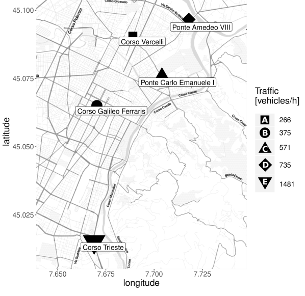
Figure 6: Considered PoPs in the environment data-set (Turin city).

In order to feed the environment with realistic traffic we collected a data-set spanning from January to October 2020 of vehicle traffic gathered in Turin (Italy). There are over 100 measuring locations distributed throughout Turin where the number of vehicles that pass each particular measuring point is counted over 5 minute intervals. At the end of every 5 minute interval, the traffic intensity (i.e., the number of vehicles arriving in that 5 minute interval divided by 5 minutes) is expressed as a number of vehicles per hour. Not all measuring points report traffic intensities for each 5 minute interval. We selected the $P=5$ stations with the maximum amount of measurements and interpolated the missing measurements (via expectation maximization). Fig. 6 shows how the measuring points (which we consider to be as PoPs in this paper) are distributed across the city.

This data-set provides us the traffic intensity $\Lambda_{p}(t)$ [vehicles/hour] at each PoP $p\in\{1,\ldots,P\}$ every 5 minutes. We use these time-varying $\Lambda_{p}(t)$ values as the arrival rates of $P$ independent Poisson processes that model vehicle arrivals on instants $t_{v}$ at the $P$ PoPs. Namely, at each time window $[t,t+5\text{min}]$ we iterate over each PoP $p$ and randomly generate its car arrivals as

$$\{t_{1},t_{2},\ldots\}=\{t_{i}\}_{i}=\left\{t+\sum_{j=0}^{i}k_{j}\right\}_{i},\quad k_{j}\sim exp\left(\Lambda_{p}(t)\right)$$ (20)

with $exp\left(\Lambda_{p}(t)\right)$ denotes the exponential distribution with rate $\Lambda_{p}(t)$. By repeating this random generation of arrivals for every PoP $p\in P$, and for every time window of 5 min; we generate a data-set with samples $\{(t_{1},p_{1}),(t_{2},p_{2}),\ldots\}$ (time $t_{v}$ of vehicle arrival at PoP $p_{v}$). This data-set drives the simulation – see $(t_{v},p_{v})$ rows Fig. 5. To gain statistical significance, we repeat 40 times the random generation of arrivals, using formula (20) with different seeds. As a result, we obtain 40 different traces that express how vehicles arrive to each PoPs in Fig. 6 between the 28^th of January, and the 1^st of October 2021.

6 Performance evaluation

TABLE III: Training and testing traces.

trace	start	end	duration	arrivals
training	Jan 28 17:55	Jan 29 07:13	13.3 hrs	28352
testing	Jan 29 07:13	Jan 29 12:43	5.5 hrs	28353

In this section we evaluate the performance of the proposed approach on the V2N service provisioning problem. Specifically, while employing the same greedy placement strategy as defined in formula (14), we study the performance of the fully decentralized approach DDPG-1 as well its centralized version DDPG-N (Fig. 4) and compare them against the scaling approaches described in Section 4. For the sake of simplicity, we denote the solutions using their associate scaling methods hereafter, as they share the same placement strategy. For instance, TES represents the solution comprises greedy placement and the TES scaling approach etc.

6.1 Experimental setup

All solutions are evaluated with the simulation environment presented in Section 5, where we use Python 3.9.12, complemented with the PyTorch 1.11.0 library. We employ the data-set described in Section 5.2 in an area of 5 PoP s. To run the experiments we use a server with Intel Core i7-10700K CPU, 32 GB of RAM.

6.2 Hyperparameters

In this subsection, we give the detailed parameter settings for the scaling agents mentioned in Section 3 and 4.

CNST. We perform a grid search to find the optimal number of CPU s for the selected PoPs (five in total) in formula (18), namely sweeping over $C_{p}$ where $p\in\{1,2,3,4,5\}$, resulting in $6^{5}=7776$ combinations. The best found combination over the training set is $(C_{1},C_{2},C_{3},C_{4},C_{5})=(1,5,5,1,5)$.

PI. We perform a grid search to find the optimal parameters $\alpha$, $\beta$ and $\rho_{tgt}$ within the ranges suggested by the authors in [5]. The best found result over the training set is $(\alpha,\beta,\rho_{tgt})=(4,0,0.7)$.

TES. TES is an adaptive algorithm that does not have a training phase. The only hyper-parameters to define are $W$ and $m$, as mentioned in Section 4.3. We set $W\cdot m=1$ second.

DDPG. DDPG-1 and DDPG-5 have similar hyper-parameter settings: the architectures of actor and critic are both a 3-layer perceptron. Each layer contains 64 neurons for DDPG-1 and 256 neurons for DDPG-5, followed by Exponential Linear Unit (ELU) [23] activation functions. The size of replay buffer consists of $1\text{\times}{10}^{6}$ entries; the discount factor is set to $\gamma=0.99$; the soft update for Polyak averaging is set to $\tau=$1\text{\times}{10}^{-3}$$. Adam optimization [24] is employed with different learning rates $\alpha_{a}=$1\text{\times}{10}^{-4}$$ and $\alpha_{c}=$1\text{\times}{10}^{-3}$$ for the actor and critic, respectively, following the settings in [12]. We notice that setting $\alpha_{c}$ larger than $\alpha_{a}$ is crucial to have the training more robust. Furthermore, a noise perturbation drawn from Gaussian distribution with $\mu=0$ and $\sigma=0.1$ is introduced to the action value during training, to encourage exploration [25]. We train both DDPG-1 and DDPG-5 for 100 episodes.

6.3 Metrics and evaluation scenarios

Our goal is to maximize the long term reward as described in formula (13) that aims at meeting the delay target without over-provisioning of resources, via finding an adequate strategy of scaling and placement over time. We run all scaling agents (coupled with the greedy placement agent described in Section 3) on the complete traces summarized in Table III and compare them on the basis of average number of active CPUs, average reward and delay violations ($>$50ms). Note that we consider a trace that is long enough to cover various traffic patterns, including peak/off-peak hours. To have statistical significance in our results, we use 40 different traces (see Section 5.2) for each experiment that span through the training or testing period. Before the actual comparisons of the approaches, we look into learning curves of DDPG-based approaches. In the following, we look more closely into the behaviour of the DDPG-based approaches at each PoP. Furthermore, we show the optimality gap with regards to the global optimal solution for Problem 1. Finally, we investigate the computation complexity of the propose approaches and compare them in terms of average run time.

6.4 Convergence of DDPG-N

Figure 7: Learning curves of DDPG-1 and DDPG-5 over the training (top) and testing (bottom) sets.

Fig. 7 shows the learning curves of DDPG-1 and DDPG-5 over 100 episodes. We report average rewards and the corresponding $95\%$ confidence intervals by repeating the experiment 10 times. We can see that DDPG-1 converges faster than DDPG-5, while having lower variance. We argue that this difference is mainly caused by their reward signals. Due to the nature of their design, DDPG-1 receives a reward by taking an action, while DDPG-5 receives a reward by taking a set of actions (for multiple PoPs) jointly. The reward for the latter is identical to the average of rewards received from all PoPs, thus the value is averaged out. This fact results in smaller gradients in optimization. Therefore, learning takes longer to converge. Moreover, no overfitting is observed during 10 epochs. We note that the final reward obtained from the testing set is higher than that of the training set due to the Gaussian noise imposed upon the training phase.

6.5 Comparison analysis

We compare the trained DDPG-1 and DDPG-5 agents against the solutions in Section 4, since the placement approach is the same. The comparison is done over the forty randomly generated periods of 5.5h in the testing trace – Formula (20) and Table III, respectively.

Figure 8: Average reward over 40 realizations of a 5.5h interval. Number annotations represent the average value, and error bars represent three times the standard deviations.

Fig. 8 illustrates the reward that each solution attained averaged over the 40 versions of the testing trace, while the error bars show three times the associated standard deviation of the reward. In Fig. 8 we see that DDPG-1 and DDPG-5 increase the average reward by $3$% and $1.5$% compared to the one attained by TES, respectively; while PI and CNST remain below TES with average rewards of $16.4$% and $20.9$%, respectively. Moreover, the behaviour of almost every solution remained fairly stable (see the error bars in Fig. 8 ) thanks to the training approach used; the parameters of every solution are selected to maximize the reward for a training trace with both off-peak and rush hours during the day, and the traffic patterns follow a seasonal trend [15]. Hence, every solution generalizes adequately despite the traffic variations of the different 40 versions of the testing trace.

To understand the rewards reported in Fig. 8 we take a look at the behaviour of every solution during rush hours in the city of Turin. In Fig. 9, we omit the CNST case, which we used as a benchmark in Fig. 8, to render the figure more readable. To further increase its readability, we smooth the traces by using Bezier curves to capture the main trends without being distracted by the small fluctuations inherent to the traces.

We first focus on the PI approach. Primarily, PI obtains a small reward due to its failure to distribute the C-V2N traffic among PoPs, since there is almost always a PoP with active 5 CPUs ($\max_{p}\{C_{p}\}=5$ during long periods in Fig. 9). A second reason is that PI has the highest number of CPUs ($\sum_{p}C_{p}$) across PoPs. And the third reason is that PI leads to the largest increase of CPUs upon traffic peaks. As an example, Fig. 9 shows that as road traffic peaks around 7:30, it leads to the highest number of active CPUs ($\sum_{p}C_{p}>20$). These three reasons hint at the over-provisioning nature of PI, for it is a conservative solution that aims at keeping loads around 0.7. This turns out to be a low value, leading to a delay that tends to be lower than the target one. Hence PI fails to obtain the best possible reward (Fig. 2).

Figure 9: Behaviour of DDPG-1/5 and other solutions as the number of vehicles change over time (bottom). From top to down we show the maximum/minimum CPUs each PoP has ($\max_{p}\{C_{p}\}$ and $\min_{p}\{C_{p}\}$, respectively), and the sum of PoP CPUs ($\sum_{p}^{5}C_{p}$).

Although Fig. 9 conveys the flaws of PI, it is not so easy to infer why DDPG-1 and DDPG-5 outperform TES. Actually, the three solutions use almost the same number of CPUs across PoPs $\sum_{p}C_{P}$. The main difference, although not that pronounced, is that DDPG-5 is more prone to overload certain PoPs. We observe that the number of CPUs for the most loaded PoP ($\max_{p}\{C_{p}\}$) remains higher than for DDPG-1 and TES (see Fig. 9 top). At the same time, DDPG-5 tends to have less CPUs in the least loaded PoP ($\min_{p}\{C_{p}\}$) compared to DDPG-1 and TES. Both facts give insights on why DDPG-5 is slightly worse than DDPG-1, however it is difficult to draw conclusions regarding the reward.

Figure 10: ePDF of experienced total delay $d_{v}$.

Figure 11: eCDF of CPUs used by all PoP s $\sum_{p}C_{p}$.

To gain a deeper understanding on the behaviour of DDPG-1, DDPG-5, and TES, we plot (i) the ePDF of the delay experienced by vehicles $d_{v}$ in Fig. 10 and (ii) the eCDF of the total number of CPUs across the five PoPs $\sum_{p}^{5}C_{p}$ in Fig. 11. For the former we resort to kernel density estimates to derive the ePDF illustration.

Fig. 10 shows that the ePDF peak of DDPG-5 is the closest to the target delay of $d_{tgt}=50$ ms. Hence, vehicles are most likely to experience delays near the target 50 ms, which translates into a higher reward (see Fig. 2). But at the same time, Fig. 10 shows that with DDPG-5 vehicles have higher chance to violate the target delay. Increased delays are due to the fact that DDPG-5 it is more likely to use less CPUs than TES and DDPG-1. Indeed, Fig. 11 shows exactly that. In other words, DDPG-5 uses less CPUs than TES and DDPG-1, thus, vehicles are experiencing higher delays.

Regarding TES and DDPG-1, Fig. 10 shows that their ePDFs are very similar. Namely, both TES and DDPG-1 have narrow ePDFs skewed to the left, i.e., most of the vehicles experience delays $d_{v}$ near the peak between 20 ms and 30 ms. As a result, TES and DDPG-1 are less likely to violate the target delay of $d_{tgt}=50$ ms as they use more CPUs than DDPG-5. Nonetheless, they both use less than 14 CPUs the 50% of the time (Fig. 11).

Overall, Fig. 10 and Fig. 11 show that the DDPG-1 actor $\theta^{\pi}$ learned a policy with a very similar behaviour to the forecast-based solution of TES. This suggests that DDPG-1 has (implicitly) learned to foresee how the traffic patterns will evolve in C-V2N communications (without having to provide it with the seasonality as in the case of TES). However, the DDPG-5 scaling agent learned a more conservative policy that uses less CPUs to support the C-V2N workload. As a result, most vehicles experience delays $d_{v}$ near the target of $d_{tgt}=50~{}ms$ and achieve high rewards, but also have higher risk of experiencing delays larger than that (thus decreasing the reward accordingly). Below we check in more detail DDPG-1 and DDPG-5 to gain a better understanding on the differences between the top two solutions (Fig. 8).

6.6 Behaviour of DDPG-N at each PoP

So far we know that DDPG-1 and DDPG-5 differ by just $0.01$ in the obtained average reward (Fig. 8). We also know that DDPG-5 is more conservative in terms of allocating CPUs than DDPG-1 (Fig. 11), hence risking more delay violations, yet remaining near the target delay (see Fig. 10). In Fig. 12 we compare the behaviour of DDPG-1 and DDPG-5 per PoP by looking at (i) the ePDF of the total delay experienced by vehicles $d_{v}$, (ii) the number of CPUs $C_{p}$, and (iii) the number of assigned vehicles $N_{p}$. As before, we resort to kernel density estimates to derive the ePDF s.

(a)

(b)

(c)

Figure 12: Comparison of DDPG-1 vs. DDPG-5 over all PoPs. We compare the ePDF of the vehicle delays $d_{v}$ (top), number of CPUs $C_{p}$ at each PoP (middle), and number of vehicles assigned to each PoP $N_{p}$ (bottom).

The first evidence we draw from Fig. 12 (bottom) is that DDPG-1 distributes the number of assigned vehicles $N_{p}$ per PoP more evenly than DDPG-5, as the highest ePDF peak is near $N_{p}=8$ for every PoP. DDPG-5 is assigning less vehicles to PoP B and more vehicles to PoP C – see how the former ePDF is skewed to the left, and the latter to the right.

The second evidence is a consequence of the former. When DDPG-5 assigns fewer vehicles to PoP B the ePDF for the number of CPUs also skews to the left in Fig. 12 (middle). In other words, as DDPG-5 assigns less vehicles to PoP B, it also uses less CPUs. Conversely, as DDPG-5 assigns the excess of vehicles to PoP C it also provisions more CPUs, around $C_{p}>4$ to be precise. This explains why on Fig. 9 (top) the maximum loaded PoP (i.e., PoP C) has more active CPUs with DDPG-5 than with DDPG-1.

The third evidence we draw from Fig. 12 (top) is that DDPG-5 is more prone to exceed the target delay of $d_{tgt}=50$ ms, as we discussed in Fig. 10. In particular, although DDPG-5 assigns few vehicles to PoP B the CPU provisioning should not be as low, for that results in a peak on the right side of the target delay $d_{tgt}$ ePDF. That is, DDPG-5 assigned too little CPUs to PoP B and this results in high probability of violating the target delay of 50 ms, as shown in the peak of Fig. 12 (top). Conversely, DDPG-1 keeps similar ePDF for the vehicle total delay $d_{v}$ across PoPs, always having a higher mass of probability below 50 ms.

Overall, the conclusions we draw from Fig. 12 highlight that DDPG-1 achieves a more balanced placement of C-V2N application tasks across the considered PoPs, while DDPG-5 assigns less vehicles to PoP B and assigns the excess to PoP C. The latter behaviour is because DDPG-5 receives as input the information of all PoPs (see Fig. 4) and prefers to send the C-V2N traffic to the PoP that already has more active CPUs.

6.7 Optimality gap

We study how far is DDPG-1 and DDPG-5 with respect to the optimal solution of Problem 1. Note that it is NP-hard (Lemma 1) thus we cannot find an optimal solution in polynomial time. Furthermore, an oracle needs to know in advance the vehicles’ arrival times $\{t_{1},t_{2},\ldots\}$ to derive the optimal solution, a condition that is not applicable in real world settings.

To understand the impact of such optimality gap, we depict how placement and scaling decisions affect the processing delay in Fig. 13. Note that to maximize the reward function $R(\cdot)$ in formula 9, the delay experienced by a vehicle $d_{v}=\mathbb{E}[l_{p_{v},p_{v}^{\prime}}]+\mathbb{E}[d_{p_{v}^{\prime},v}]$ must be as close as possible to the target delay $d_{tgt}=50$ ms. In other words, the placement and scaling solution should avoid under/over-provisioning computing resources. Fig. 13 shows the processing delay $d_{p}$ in a PoP as the number of assigned vehicles $N_{p}$ and CPUs $C_{p}$ increase. Using circles, we highlight the maximum processing delay before exceeding the target of 50 ms. For example, with $C_{p}=3$ the PoP can process on time C-V2N traffic of $N_{p}=10$ vehicles. If the number of vehicles increase, then an additional CPU should be activated. On top of the processing delay illustrated in Fig. 13, one must add also the transmission delay $l_{p_{v},p_{v}^{\prime}}$, whenever a task is assigned to a PoP that is not in the vicinity of the vehicle.

Figure 13: Experienced processing delay $d_{p}$ at a PoP as the number of assigned vehicles $N_{p}$ and CPUs (lines) increase.

To derive the optimal solution for Problem 1, we use AMPL [11] to encode the problem, and KNITRO [26] to solve it. The search space explodes as we increase the time horizon, i.e., as we increase the number of vehicles $V$ considered with their respective arrivals $t_{v},\ v\in V$. Specifically, the search space grows at a pace of $\mathcal{O}(\mathcal{A}^{|V|})$ – with $\mathcal{A}$ the action space detailed in (12). The vast search space makes the problem computationally intractable. As an example, with 4 Intel Xeon CPUs KNITRO does not manage to find an optimal solution within 65h for a problem instance with $|V|=81$ vehicles.

TABLE IV: Small scale evaluation

Algorithm	avg gap (%)	avg $\#$CPUs	% delay violations
Optimal	-	0.3	3%
DDPG-1	25.5%	0.37	10%
TES	35.7%	0.5	10%
PI	44.9%	0.4	27%
DDPG-5	57.1%	0.77	40%
CNST	78.6%	3.4	0%

To find a tractable instance of the problem, we decrease the number of vehicles to the first $|V|=6$ vehicles that arrive in the testing set.

In Table IV we compare the performance of the proposed approaches for the aforementioned small scale evaluation scenario, in terms of the average gap to the optimal solution. Furthermore, for each solution we list the average number of CPUs activated over the simulation period and the corresponding percentage of delay violations. DDPG-1 exhibits the lowest (25.51%) optimality gap compared to the rest of the approaches under evaluation. Table IV also shows that DDPG-1 is the solution that minimizes the average number of CPUs and delay violations in the considered C-V2N service. We also observe a small percentage of delay violations for the optimal solution due to the soft delay constraint, as defined in the objective function. On the other extreme, the CNST solution keeps V2N service delay below the target value, as it significantly over-provisions edge computing resources (approximately 78% compared to the optimal). Although at this point of time for the system the average gap to the optimal is considerable, we expect that the optimality gap of DDPG-1 and DDPG-5 will shrink with time assuming a large scale evaluation, as these scaling agents are trained to maximize the average reward over time (formula (13)).

6.8 Complexity Analysis

TABLE V: Algorithms run-time complexity.

	DDPG-N	PI	TES
run time	$\mathcal{O}(\eta^{2}H)$	$\mathcal{O}(P)$	$\mathcal{O}(P)$

In this section we provide the complexity analysis of each algorithm evaluated in this paper. Specifically, we derive the worst-case run time analysis of the proposed DDPG, PI, and TES.

DDPG-based approach. After completion of the training stage, Algorithm 1 places vehicles’ application tasks using $\operatorname*{argmin}_{p\in P}(l_{p_{v},p}+d_{p})$. Overall, the placement stage has runtime complexity $\mathcal{O}(P)$.

Right after the application task placement, Algorithm 1 uses the trained DDPG Actor $\theta^{\pi}$ for scaling resources – see Fig. 3. Each of the fully-connected layers of the Actor network $\theta^{\pi}$ performs a vector-matrix multiplication $\pi_{i}\cdot h_{i-1}$ to do the forward pass – with $\pi_{i}\in\mathbb{R}^{\eta_{i}\times\eta_{i}}$ being the weights of the $i$^th hidden layer with $h_{i}$ neurons, $\eta_{i}$ the number of neurons at the $i$^th hidden layer, and $h_{i-1}\in\mathbb{R}^{\eta_{i}}$ the output vector of the $i-1$^th hidden layer. If we denote $\eta=\max_{i}\eta_{i}$ as the number of neurons of the largest hidden layer, and $H$ as the number of hidden layers; then a forward pass of the Actor network $\theta^{\pi}$ is $\mathcal{O}(\eta^{2}H)$.

Note that a DDPG-$P$ Actor network receives as input the system status $s_{v}\in\mathbb{N}^{2P}$, with $P$ the number of PoP s considered in the system. Since the number of neurons in the hidden layers is typically larger than the input size $\eta>>P$, the run time of the forward pass in the scaling agent at Algorithm 1 can be expressed as $\mathcal{O}(\eta^{2}H)$. Overall, the run-time complexity of the proposed Algorithm 1 is governed by the Actor $\theta^{\pi}$ forward pass. Consequently, DDPG-based scaling Algorithm 1 has run-time complexity $\mathcal{O}(\eta^{2}H)$.

PI-based approach. The PI solution employs formula (19) so each PoP remains near the target load $\rho_{tgt}$. Prior to that scaling step, the vehicles application tasks are placed in a greedy fashion to the least loaded server – as in Algorithm 1. As the PI step in (19) and the placement operation have run-time complexity $\mathcal{O}(P)$, the PI based service provisioning solution has overall run-time complexity $\mathcal{O}(P)$ as well.

TES-based approach. The analyzed TES-based approach is based on predicting the future traffic flow $f_{p,t+1},\ldots,f_{p,t+W}$ at each PoP $p$ in a window of length $W$. Such prediction is derived using TES with additive seasonality [16]:

$$s_{p,0} =f_{p,0}$$ (21)

$$s_{p,t} =\alpha(f_{p,t}-c_{p,t-L})+(1-\alpha)(s_{p,t-1}+b_{p,t-1})$$ (22)

$$b_{p,t} =\beta(s_{p,t}-s_{p,t-1})+(1-\beta)b_{p,t-1}$$ (23)

$$c_{p,t} =\gamma(f_{p,t}-s_{p,t-1}-b_{p,t-1})+(1-\gamma)c_{p,t-L}$$ (24)

$$f_{p,t+W} =s_{p,t}+Wb_{p,t}+c_{p,t-L+1+(W-1)\bmod L}$$ (25)

with $L$ being the seasonality of the traffic flow (one day), $s_{p,t}$ the TES level, $b_{p,t}$ the trend, and $c_{p,t}$ the additive seasonality – e.g., how much we add to the flow depending on the time of the day we are at. Based on Section 4.3, $f_{p,t+W},\ \forall p$ is computed right after a window of $W$ seconds expire. To derive $f_{p,t+W}$ it takes $\mathcal{O}(1)$ operations, and the prediction is performed on each PoP $p$. Thus we conclude that the run-time complexity of the TES-based approach is $\mathcal{O}(P)$.

Figure 14: Average run time of each algorithm when performing the placement and scaling in the considered 5 PoP s upon the arrival of a vehicle.

Overall, the DDPG solutions have higher run-time complexity, as shown in Fig. 14, which illustrates the average run-time of each algorithm for the experiments conducted in Sub-sections 6.4-6.6. Nevertheless, they still achieve run-times in the sub-msec range. Thus, the proposed DDPG solutions are suitable for C-V2N services with strict latency requirements. Note that taking $\leq 300\mu$s to perform the placement and scaling is fast enough for C-V2N services with down to $d_{tgt}=10$ms latency requirements – not to mention the considered service in Section 6, with $d_{tgt}=50$ms.

6.9 Discussion

Figure 15: Tail of vehicles’ latency $d_{v}$ ePDF. Prominent peaks on DDPG-1 are due to CPU overload $\rho_{p}>1$ on multiple PoP s.

Figure 16: Candidate rewards for future work $R^{*}(d;\sigma,K)$, and the reward $R(d)$ used in our experiments. $R^{*}(d;\sigma,K)$ alike rewards will punish more the under-provisioning, i.e. $d>d_{tgt}$.

We hereby discuss the implications of the evaluation of the proposed approach for task placement and scaling of edge resources.

The fact that we couple task placement and scaling decisions, instead of addressing it as a joint problem, leads to sub-optimal solutions as we observed in Section 6.7. A DRL approach (i.e., DDPG) that would take both placement and scaling decisions – formula (12) – would account for their correlations, hence would avoid under/over-provisioning computational resources, addressing performance requirements. Furthermore, the reward function in formula (9), does not decay fast when the experienced delay exceeds the target – see $d>d_{tgt}$ values in Fig. 2. Although the DDPG-based agents learn to scale so as to meet approximately the target delay $d=d_{tgt}$, we can still observe extreme delay values with very small probability as the prominent peaks indicate in Fig. 15, which is showing the full delay range of Fig. 10 for DDPG-1. We assume that a faster decay in the reward for $d>d_{tgt}$ may reduce the chances of overloading, thus preventing delay violations. In this direction the following reward function is provided as an example, also illustrated in Fig. 16.

$$R^{*}(d;\sigma,K)=\begin{cases}R(d),&d<d_{tgt}\\ \frac{K}{\sigma}\frac{\phi\left(\frac{d-d_{tgt}}{s}\right)}{\Phi\left(\frac{b-d_{tgt}}{\sigma}\right)-\Phi\left(\frac{a-d_{tgt}}{\sigma}\right)},&d\geq d_{tgt}\end{cases}$$ (26)

with $d\geq d_{tgt}$ being a $K$-scaled truncated normal distribution [27] in the interval $[a,b]=\mathbb{R}^{+}$, centered at $d_{tgt}$ with standard deviation $\sigma$; $\phi(x)=1/\sqrt{2\phi}\exp(-\tfrac{1}{2}x^{2})$; and $\Phi(x)=\tfrac{1}{2}(1+\operatorname{erf}(x/\sqrt{2\pi}))$. Note that the $K$ scaling is set to ensure the reward continuity, i.e. $\lim_{\varepsilon\to 0}R^{*}(d+\varepsilon;\sigma,K)=\lim_{\varepsilon\to 0}R^{*}(d-\varepsilon;\sigma,K)$. Moreover, $R^{*}(d;\sigma,K)$ is differentiable at $d=d_{tgt}$ to help learning stability.

Moreover, we expected DDPG-5 to achieve a higher reward than the fully decentralized approach DDPG-1, as it uses global information (states of all considered PoP s) as input, while the DDPG-1, uses only local information. We assume that the inferior performance of DDPG-5 is due to the fact that the considered PoP s in Turin are scattered over the city, far from each other – see Fig. 6. In this case, the traffic pattern of one PoP is not tightly correlated to the traffic patterns of other PoP s. As a result, the information from other PoP s becomes redundant and thus makes learning more challenging. On the contrary, DDPG-1 does not receive uncorrelated traffic as input, hence, it focuses scaling to each PoP characteristics. Nevertheless, we conjecture that DDPG-5 may outperform DDPG-1 when dealing with PoP s that are geographically closer. To verify this idea, we run DDPG-1 and DDPG-5 on a different set of 5 adjacent stations, following the same settings of the simulation environment described in Section 5. The result shows that DDPG-5 outperforms DDPG-1 by 7.69% obtaining a reward of 0.70, which is in line with our hypothesis. Thus, service providers should carefully select the DDPG-based agent based on the geographical dispersion of PoP s.

7 Related work

In line with the development of ML techniques, different standardization bodies also started to consider and include the use of ML methods into their architecture specification and roadmaps. The Third Generation Partnership Project (3GPP) has started exploring Artificial Intelligence (AI) and ML technologies for 5^th generation (5G) systems across the Radio Access Network (RAN) and core domain and in the management plane. In the RAN domain, the O-RAN Alliance defined [28] non-Real-Time (RT) and near-RT Radio Intelligent Controller (RIC) [29, 30] to empower self-driving, leveraging new learning-based technologies to automate operational network functions and reduce operational costs. Similarly, the European Telecommunications Standards Institute (ETSI)’s Industry Specification Group (ISG) Experiential Network Intelligence (ENI) [31] focuses on AI-enabled network management and proposed the cognitive network management system based on AI, which allows operators to improve the flexibility in the network operation, by automating network configuration and monitoring processes. The goal is to achieve a seamlessly network automation, as envisioned by ETSI Zero touch network & Service Management (ZSM) [32], which focuses on network service automation and is working on the definition of a network architecture that supports various functionality such as the end-to-end network service management and network slice as a service. In addtion to the 3GPP and ETSI, the International Telecommunication Union - Telecommunication standardization sector (ITU-T) Focus Group on Autonomous Networks (FGAN) also studies how to apply ML for building autonomous networks.

With the increasing number of available data sets and growing maturity of the AI/ML techniques in recent years, it is feasible to achieve the standarization community vision of building autonomous networks using ML solutions. In this direction, there have been quite some research work of adopting the AI/ML algorithms to solve service function chain (SFC) placement problem, that is quite similar to the service task placement problem in this paper. Traditional solutions mostly use mathematical models or heuristic methods, which are usually not applicable in the context of large-scale networks. Leveraging intelligent learning algorithms, efficient solutions can automatically adapt to changes in the dynamic network environment and service load through learning. For example [33] proposes a joint optimization approach of flow path selection and VNF placement, which explores the best utilization of bandwidth to reduce network delay for delay-sensitive applications. Authors employ Reinforcement Learning, while they use both the flow path delay and network function-related delay for the estimating the reward for placing VNFs. Similarly, [34] presents a multi-objective optimization SFC placement algorithm based on reinforcement learning. The goal of the algorithm is to optimize resource allocation, considering several performance metrics. The authors model the problem as an MDP, and use a two-layer policy network as an intelligent agent. Authors in [35] employ a Deep Q-Learning (DQL) approach to address admission control for the SFC placement problem. The SFC placement problem has been also investigated in the context of Edge-enabled 5G/6G networks. For instance [36] develops a practical solution using Q-Learning, considering both computational and communication resources when placing VNFs in the network.

In the area of resource scaling, authors in [37] classify the scaling techniques as either schedule-based or rule-based solutions, with the latter being related to auto scaling methods. Specifically, authors in [37] show that threshold-based policies, queuing theory, control theory, time-series analysis, and RL are candidates for rule-based auto scaling. However, among the prior rule-based auto scaling solutions RL is not the only AI/ML approach – as pointed out by [38]. Some works propose using classification-based ML solutions [39] that tell whether the current network status lies within a category that requires to scale up; and other works [40] propose to forecast the future network demand to trigger an Integer Linear Programming (ILP) solver that takes provisioning and scaling decisions.

Forecasting the future traffic demand is actually the most proliferous approach, since an accurate estimation of the incoming demand provides rich insights to anticipate the scaling operation. Works in the literature forecast the future demand resorting to classic time-series techniques such as AutoRegressive Integrated Moving Average (ARIMA) or TES [16, 41], Neural Network (NN) solutions based on Long Short Term Memory (LSTM) cells [42, 43], convolutional neural networks [44], or even Graph Neural Network (GNN) s [45]. Such approaches have been successfully used in the context of effective network slicing [46, 47, 48] and cloud dimensioning [49]. But despite the context where forecasting is used, it is important to keep in mind that AI/ML approaches require large amounts of data and computing resources, whilst traditional time-series approaches do not. Thus, the interest of works as [15, 5]is comparing the trade-offs between traditional and AI/ML solutions for forecast-assisted scaling.

In the context of Vehicle-to-Everything (V2X) services, there is a rich literature on how to use AI/ML solutions to automatically scale radio resources. Authors in [47] propose an autoencoder and Convolutional Neural Network (CNN) architecture that detects incoming road events to allocate radio resources for different slices (infotainment or emergency services). Authors in [50] resort to DQN [51] to provision radio resources for Vehicle-to-Vehicle (V2V) services, while [52] assesses channel resource allocation for V2X services using a blend of LSTM with Advantage Actor-Critic (A2C) and Deep Q-Network (DQN). Authors in [53] use A2C and Proximal Policy Optimization (PPO) to select the radar channel, such that the age of information of high priority notifications is minimized. However, all the aforementioned works use AI/ML to auto scale or manage the wireless resources for vehicular networks. To the best of our knowledge, approaches studied in this context neglect that fact that edge computing resources should also scale with the increase in vehicular service demand. There are however cases where either servers with fixed resources are considered [54], or BS s are associated with slices that offer static computational resources [55]. Moreover, existing approaches address the function/task placement and scaling problems separately. Our work advances the state-of-the-art by jointly assessing task placement and scaling of computational resources coupling the two problems and considering their inter-dependency, to support C-V2N applications at scale over a city area spanning multiple PoP s. Furthermore, we employ DDPG rather than the widely used A2C agents to scale edge computing resources and prove its efficiency and applicability in both centralized and decentralized decision making modes.

8 Conclusion

In this paper we studied C-V2N service provisioning supported by the edge cloud. More specifically, we propose a decentralized approach for C-V2N application task placement and scaling of edge computing resources. In each PoP a placement and scaling agent is running: the former is responsible for placing the tasks associated to a vehicle to the most appropriate PoP, while the latter is dealing with activating and deactivating CPUs resources in each PoP, to efficiently support the C-V2N application. To promote cost effective use of the edge resources and avoid overbooking them at PoP level, application tasks of a vehicle arriving in the vicinity of one PoP can be processed at a nearby PoP in the service area, taking into account the additional transmission delay. Both sets of agents take their decisions based on the delay that the tasks experience. To address task placement we use a greedy approach, while for making scaling decisions we develop DDPG-based approaches; a fully decentralized one where scaling decisions are taken at each PoP separately (DDPG-1) and a centralized version where the scaling agent make a decision for all the PoP s in the area denoted as DDPG-N .

We compare the performance of these scaling approaches against state-of-the-art ones that base their decisions on the load that is observed rather than on the delays. The first one is a traditional PI controller, while the second one, TES, scales based on predictions for the service load. We found that the PI approach is too conservative, keeping the load (thus delay) quite low and consequently demanding more edge resources. The TES approach performs slightly worse than the DDPG ones, but it relies on being provided with the exact period of seasonality. In other words, the DDPG approaches are able to learn the seasonality themselves without requiring it as an additional input parameter. Comparing the centralized version of the DDPG (DDPG-5) to the decentralized one (DDPG-1), we conclude that the latter performs slightly better, as is distributes the loads more evenly over the various PoPs and in turn results in higher average reward and less delay violations. Furthermore, DDPG-1 requires no synchronization of the information regarding the workload and resource dynamics for the rest of the PoPs. Finally, we compared our solution to the optimal one that employs full knowledge of all vehicles’ arrivals in the future. Our proposed solution presents a 25% optimality gap. Although the comparison is somewhat unfair as our solution is only based on causal information, it hints the fact that there is still room for improvement.

In future work we plan to tackle the identified gaps of the proposed DDPG-based agents by $(i)$ incorporating the task placement decisions into the DDPG-based agents to solve both placement and scaling problems in one single model; ($ii$) adjusting the reward shape when $d>d_{tgt}$ to tune the degree of allowed SLA violation; and ($iii$) investigating solutions working on a larger number of PoP s that involves varying degrees of correlation between them.

Appendix A Proof of Lemma 1

Proof.

We proof the $\mathcal{NP}$-hardness of Problem 1 (Section 2.2) by showing that an instance of our problem is equivalent to the generalized assignment problem [56].

Let us consider an instance of Problem 1 that we want to solve for a time window $T$, in particular, we take a problem instance with every vehicle departing after the considered time window, i.e, $T_{v}>T$ holds $\forall v$.

When a vehicle $v$ arrives to the vicinity of PoP $p_{v}$ we have to take a placement decision to know that the C-V2N tasks of vehicle $v$ will be processed at PoP $p^{\prime}_{v}$. Note that the C-V2N tasks of vehicle $v$ will induce a CPU increase $C_{v,p^{\prime}_{v}}^{+}$ at PoP $p^{\prime}_{v}$ to maximize the reward (i.e., to stay close to the target delay $d_{tgt}$ in Fig. 2). Namely, the CPU increase is expressed as:

$$C_{v,p_{v}^{\prime}}^{+}=\operatorname*{argmax}_{C}\left\{R(C,p_{v}^{\prime},N_{v-1,p_{v}^{\prime}}+1)\right\}\\ -\operatorname*{argmax}_{C}\left\{R(C,p_{v}^{\prime},N_{v-1,p_{v}^{\prime}})\right\}$$ (27)

with $N_{v-1,p_{v}^{\prime}}+1$ capturing that PoP $p_{v}^{\prime}$ will accommodate the tasks of an additional vehicle, i.e., vehicle $v$. Note how in formula (27) we make explicit the dependence on the number of vehicles $N_{v,p_{v}^{\prime}}$ within the reward function for the latter depends on the average processing delay $d_{p,v}$ experienced by the vehicle, which is impacted by $N_{v,p_{v}^{\prime}}$ defined (Section 2.1) as:

$$\mathbb{E}[d_{p,v}]=\begin{cases}\frac{1}{\mu(C_{p,v})-\lambda N_{p,v}}&\mbox{if $\mu(C_{p,v})>\lambda N_{p,v}$}\\ \infty&\mbox{otherwise}\end{cases}$$ (28)

With the PoP CPU increase by each vehicle (27) we reformulate Problem 1 as:

$$\max_{p^{\prime}_{v}} \sum_{v}\sum_{p}R(C_{p,v},p_{v}^{\prime},N_{p})\mathds{1}_{p^{\prime}_{v}}(p)$$ (29)

$$s.t.: \sum_{v}C_{v,p_{v}^{\prime}}^{+}\mathds{1}_{p_{v}^{\prime}}(p)\leq C_{p}^{\max},\quad\forall p$$ (30)

$$p^{\prime}_{v}\in P$$ (31)

We now indicate how the variables/parameters in the formulation above mimic to the notation used in the generalized assignment problem [56]. First, we take $x_{v,p}=\mathds{1}_{p^{\prime}_{v}}(p)$ as the binary variable telling whether vehicle $v$ C-V2N tasks are processed at PoP $p$. Second, we write $R_{v,p}=R(C_{p},p_{v}^{\prime},N_{p})$ as the profit/reward obtained by having PoP $p$ processing vehicle $v$ C-V2N tasks. Third, we denote $w_{v,p}=C_{v,p}^{+}$ as the CPU “weight” that vehicle $v$ brings in to PoP $p$ in terms of additional CPU s. Finally, we note that (31) means that every vehicle $v$ C-V2N tasks must be processed at one PoP within the set $P$, i.e., $\sum_{p}x_{v,p}=1$ must hold $\forall v\in V$. Overall, our reduction in (29)-(31) becomes:

$$\max \sum_{v}\sum_{p}p_{v,p}\cdot x_{v,p}$$ (32)

$$s.t.: \sum_{v}w_{v,p}\cdot x_{v,p}\leq C_{p}^{\max},\quad\forall p$$ (33)

$$\sum_{p}x_{v,p}=1,\quad\forall p$$ (34)

which is the generalized assignment problem with vehicles $v$ being items that we have to place at a certain bins/PoP s $p$. In our case the profit is our reward function, and the bins’ capacity is $C_{p}^{\max}$.

Therefore, we have found an instance of Problem 1 that is equivalent to the generalized assignment problem [56], which is $\mathcal{NP}$-hard. As a consequence, Problem 1 is also $\mathcal{NP}$-hard.

∎

Appendix B Target latency

Figure 17: Ratio of M/D/1-PS percentile latency $d^{\kappa}_{p,v}$ and M/G/1-PS average latency $\mathbb{E}[d_{p,v}]$ as the CPU load $\rho$ increases. Results are obtained with the CIW simulator [57].

In this paper we simulate an Advanced Driving V2N service, and set the target latency to be $d_{tgt}=50$ ms. According to [2] [18], advanced driving services have a latency requirement between 10 and 100 ms, and a reliability in between a 90 and 99.999%.

Note, however, that our model and simulation consider average latency – see formulas (3) and (4) in Section 2.1. Consequently, the proposed and evaluated solutions of Section 6 aim to meet average service delay of 50 ms, rather than meeting the 10 to 100 ms latency requirement the 90 or 99.999% of the times. Nevertheless, the results apply to the real service requirements as we explain in the following paragraphs.

Our simulator and system model assumes that servers follow an M/G/1-PS discipline to attend the vehicles demand – see (28). However, video decoding and video recognition tasks have associated deterministic service times – see [19] and [20], respectively. Thus, the vehicle video will be attended in CPUs with an M/D/1-PS discipline, and the service times are the ones reported in Table 2 (Section 5.1)

Fig. 17 shows the relation between the $\kappa$^th sojourn time percentile (latency) in M/D/1-PS systems (denoted as $d^{\kappa}_{p,v}$), and the average sojourn time in M/G/1-PS systems ($\mathbb{E}[d_{p,v}]$). Results show that for the $\kappa=99$ percentile the ratio is at most two $d^{\kappa}_{p,v}/\mathbb{E}(d_{p,v})\leq 2$, which means that the 99^th percentile of the latency experienced by vehicles with M/D/1-PS servers is, at most, two times the average latency experienced when using M/G/1-PS servers.

Hence, the average target latency considered in Section 6 experiments $d_{tgt}=50$ ms is equivalent of meeting a 100 ms latency requirement the 99% of the times, and Section 6 meets the standard requirements [2, 18].

Cyril Shih-Huan Hsu is a Ph.D. candidate in the Informatics Institute, University of Amsterdam (UvA), The Netherlands, since 2021. He received the B.Sc. and M.Sc. degrees from National Taiwan University (NTU), in 2013 and 2015, respectively. From 2016 to 2021, he worked for several international AI startups as a machine learning researcher. He is currently a member of the Multiscale Networked Systems Group (MNS) that focuses on programmable networks and data-centric automation. His recent research focus on network resource management with AI/ML.

Jorge Martín Pérez obtained a B.Sc in mathematics, and a B.Sc in computer science, both at Universidad Autónoma de Madrid (UAM) in 2016. He obtained his M.Sc. and Ph.D in Telematics from Universidad Carlos III de Madrid (UC3M) in 2017 and 2021, respectively. His research focuses in optimal resource allocation in networks, and since 2016 he participates in EU funded research projects in UC3M Telematics department.

Danny De Vleeschauwer obtained an MSc. in Electrical Engineering and the Ph.D. degree in applied sciences from the Ghent University, Belgium, in 1985 and 1993 respectively. Currently, he is a DMTS in the access network control department of Nokia Bell Labs in Antwerp, Belgium. Prior to joining Nokia, he was a researcher at Ghent University. His early work was on image processing and on the application of queuing theory in packet-based networks. His current research focus is on the distributed control of applications over packet-based networks.

Koteswararao Kondepu is an Assistant Professor at India Institute of Technology Dharwad, Dharwad, India. He obtained his Ph.D. degree in Computer Science and Engineering from Institute for Advanced Studies Lucca (IMT), Italy in July 2012. His research interests are 5G, optical networks design, energy-efficient schemes in communication networks, and sparse sensor networks.

Luca Valcarenghi is an Associate Professor at the Scuola Superiore Sant’Anna of Pisa, Italy, since 2014. He published almost three hundred papers (source Google Scholar, May 2020) in International Journals and Conference Proceedings. Dr. Valcarenghi received a Fulbright Research Scholar Fellowship in 2009 and a JSPS ”Invitation Fellowship Program for Research in Japan (Long Term)” in 2013. His main research interests are optical networks design, analysis, and optimization; communication networks reliability; energy efficiency in communications networks; optical access networks; zero touch network and service management; experiential networked intelligence; 5G technologies and beyond.

Xi Li received her M.Sc in electronics and telecommunication engineering from Technische Universität Dresden in 2002 and her Ph.D. from the University of Bremen in 2009. Between 2003 and 2014 she worked as a research fellow and lecturer at the Communication Networks Group in the University of Bremen, leading a team working on several industrial and European R&D projects on 3G/4G mobile networks and future Internet design. From 2014 to 2015 she worked as a solution designer in Tele-fonica Germany GmbH & Co. OHG, Hamburg. Since March 2015 she has been a senior researcher in 5G Networks R&D at NEC Laboratories Europe.

Chrysa Papagianni is an assistant professor at the Informatics Institute of the University of Amsterdam. She is part of the Multiscale Networked Systems group that focuses its research on network programmability and data-centric automation. Prior to joining UvA she was a network research engineer for Bell Labs Antwerp, as part of the end-to-end Network Service Automation lab. From 2016 to 2018 she was a Research Scientist for the Institute for Systems Research, at the University of Maryland in the United States. Her research interests lie primarily in the area of programmable networks with emphasis on network optimization and the use of machine learning in networking. She has participated in various EU FIRE and 5G-PPP projects, such as Fed4FIRE+, OpenLab, NOVI and 5Growth working on issues related to network slicing.

References

- [1] 3GPP TS 23.28, “Architecture enhancements for V2X services (Release 16),” Tech. Rep., March 2019.
- [2] “Technical Specification Group Services and System Aspects;Enhancement of 3GPP support for V2X scenarios;,” 3GPP, Technical Specification 22.186.v17.0.0, April 2022.
- [3] M. H. C. Garcia, A. Molina-Galan, M. Boban, J. Gozalvez, B. Coll-Perales, T. Şahin, and A. Kousaridas, “A Tutorial on 5G NR V2X Communications,” IEEE Communications Surveys Tutorials, vol. 23, no. 3, pp. 1972–2026, 2021.
- [4] F. Giannone, P. A. Frangoudis, A. Ksentini, and L. Valcarenghi, “Orchestrating heterogeneous MEC-based applications for connected vehicles,” Computer Networks, vol. 180, p. 107402, 2020. [Online]. Available: https://www.sciencedirect.com/science/article/pii/S1389128620301997
- [5] D. De Vleeschauwer, J. Baranda, J. Mangues-Bafalluy, C. F. Chiasserini, M. Malinverno, C. Puligheddu, L. Magoula, J. Martín-Pérez, S. Barmpounakis, K. Kondepu, L. Valcarenzhi, X. Li, C. Papagianni, and A. Garcia-Saavedra, “5Growth Data-Driven AI-Based Scaling,” in 2021 Joint European Conference on Networks and Communications 6G Summit (EuCNC/6G Summit), June 2021, pp. 383–388.
- [6] A. Islam, A. Debnath, M. Ghose, and S. Chakraborty, “A survey on task offloading in multi-access edge computing,” Journal of Systems Architecture, vol. 118, p. 102225, 2021.
- [7] F. Malandrino, C. F. Chiasserini, G. Einziger, and G. Scalosub, “Reducing Service Deployment Cost Through VNF Sharing,” IEEE/ACM Transactions on Networking, vol. 27, no. 6, pp. 2363–2376, 2019.
- [8] R. Cohen, L. Lewin-Eytan, J. S. Naor, and D. Raz, “Near optimal placement of virtual network functions,” in 2015 IEEE Conference on Computer Communications (INFOCOM), 2015, pp. 1346–1354.
- [9] S. Agarwal, F. Malandrino, C.-F. Chiasserini, and S. De, “Joint VNF Placement and CPU Allocation in 5G,” in IEEE INFOCOM 2018 - IEEE Conference on Computer Communications, 2018, pp. 1943–1951.
- [10] D. P. Heyman and M. J. Sobel, Stochastic models in operations research. 1. Stochastic processes and operating characteristics. McGraw-Hill New York, NY, USA:, 1982.
- [11] R. e. a. Fourer, “AMPL. A modeling language for mathematical programming,” 1993.
- [12] T. P. Lillicrap, J. J. Hunt, A. Pritzel, N. Heess, T. Erez, Y. Tassa, D. Silver, and D. Wierstra, “Continuous control with deep reinforcement learning,” 2015. [Online]. Available: https://arxiv.org/abs/1509.02971
- [13] C. S.-H. Hsu, J. Martín-Pérez, C. Papagianni, and P. Grosso, “V2N Service Scaling with Deep Reinforcement Learning,” in IEEE Network Operations and Management Symposium (NOMS), 2023. [Online]. Available: https://arxiv.org/abs/2301.13324
- [14] R. S. Sutton and A. G. Barto, Reinforcement learning: An introduction. MIT press, 2018.
- [15] J. Martín-Pérez, K. Kondepu, D. De Vleeschauwer, V. Reddy, C. Guimarães, A. Sgambelluri, L. Valcarenghi, C. Papagianni, and C. J. Bernardos, “Dimensioning V2N Services in 5G Networks Through Forecast-Based Scaling,” IEEE Access, vol. 10, pp. 9587–9602, 2022.
- [16] P. R. Winters, “Forecasting sales by exponentially weighted moving averages,” Management science, vol. 6, no. 3, pp. 324–342, 1960.
- [17] “5GROWTH scaling,” https://github.com/MartinPJorge/5growth-scaling/blob/master/FiftyStations/clean0326/FiftyStationsEnvironment_v3.py, 2020.
- [18] M. H. C. Garcia, A. Molina-Galan, M. Boban, J. Gozalvez, B. Coll-Perales, T. Şahin, and A. Kousaridas, “A Tutorial on 5G NR V2X Communications,” IEEE Communications Surveys & Tutorials, vol. 23, no. 3, pp. 1972–2026, 2021.
- [19] M. Alvarez-Mesa, C. C. Chi, B. Juurlink, V. George, and T. Schierl, “Parallel video decoding in the emerging HEVC standard,” in 2012 IEEE International Conference on Acoustics, Speech and Signal Processing (ICASSP), 2012, pp. 1545–1548. [Online]. Available: https://doi.org/10.1109/ICASSP.2012.6288186
- [20] A. Shustanov and P. Yakimov, “CNN Design for Real-Time Traffic Sign Recognition,” Procedia Engineering, vol. 201, pp. 718–725, 2017, 3rd International Conference “Information Technology and Nanotechnology”, ITNT-2017, 25-27 April 2017, Samara, Russia. [Online]. Available: https://www.sciencedirect.com/science/article/pii/S1877705817341231
- [21] “5G; Vehicle-to-everything (V2X); Media handling and interaction,” ETSI, Sophia Antipolis - FRANCE, Standard, March 2020.
- [22] B. Coll-Perales, M. d. C. Lucas-Estañ, T. Shimizu, J. Gozalvez, T. Higuchi, S. Avedisov, O. Altintas, and M. Sepulcre, “End-to-End V2X Latency Modeling and Analysis in 5G Networks,” January 2022.
- [23] D.-A. Clevert, T. Unterthiner, and S. Hochreiter, “Fast and Accurate Deep Network Learning by Exponential Linear Units (ELUs),” 2015. [Online]. Available: https://arxiv.org/abs/1511.07289
- [24] D. P. Kingma and J. Ba, “Adam: A Method for Stochastic Optimization,” 2014. [Online]. Available: https://arxiv.org/abs/1412.6980
- [25] S. Fujimoto, H. van Hoof, and D. Meger, “Addressing Function Approximation Error in Actor-Critic Methods,” 2018. [Online]. Available: https://arxiv.org/abs/1802.09477
- [26] R. A. Waltz and J. Nocedal, “KNITRO 2.0 User’s Manual,” pp. 33–34, 2004.
- [27] Johnson, Norman L and Kotz, Samuel and Balakrishnan, Narayanaswamy, Continuous univariate distributions. John wiley & sons, 1995, vol. 289.
- [28] O-RAN alliance, “O-RAN: Towards an Open and Smart RAN,” 2018. [Online]. Available: https://www.o-ran.org/resources
- [29] A. Garcia-Saavedra and X. Costa-Pérez, “O-RAN: Disrupting the Virtualized RAN Ecosystem,” IEEE Communications Standards Magazine, vol. 5, no. 4, pp. 96–103, 2021.
- [30] M. Polese, L. Bonati, S. D’Oro, S. Basagni, and T. Melodia, “Understanding O-RAN: Architecture, Interfaces, Algorithms, Security, and Research Challenges,” 2022. [Online]. Available: https://arxiv.org/abs/2202.01032
- [31] ETSI, “Experiential Networked Intelligence (ENI); System Architecture,” European Telecommunications Standards Institute (ETSI), Group Specification (TS) 005.v2.1.1, 12 2021.
- [32] ——, “Zero-touch network and Service Management (ZSM); End-to-end management and orchestration of network slicing,” European Telecommunications Standards Institute (ETSI), Group Specification (TS) 003.v1.1.1, 06 2021.
- [33] Q. Lyu, Y. Zhou, Q. Fan, Y. Lyu, X. Zheng, G. Xu, and J. Li, “JOSP: Joint Optimization of Flow Path Scheduling and Virtual Network Function Placement for Delay-Sensitive Applications,” Mobile Networks and Applications, vol. 27, p. 1642–1658, 2022.
- [34] H. Liu, S. Ding, S. Wang, G. Zhao, and C. Wang, “Multi-objective Optimization Service Function Chain Placement Algorithm Based on Reinforcement Learning,” Journal of Network and Systems Management, vol. 30, no. 58, 2022.
- [35] T. J. Wassing, D. De Vleeschauwer, and C. Papagianni, “A machine learning approach for service function chain embedding in cloud datacenter networks,” in 2021 IEEE 10th International Conference on Cloud Networking (CloudNet). IEEE, 2021, pp. 26–32.
- [36] C. R. de Mendoza, B. Bakhsh, E. Zeydan, and J. Mangues-Bafalluy, “Near Optimal VNF Placement in Edge-Enabled 6G Networks,” in 25th Conference on Innovation in Clouds, Internet and Networks (ICIN), 2022, pp. 136–140.
- [37] S. Verma and A. Bala, “Auto-Scaling Techniques for IoT-Based Cloud Applications: A Review,” Cluster Computing, vol. 24, no. 3, p. 2425–2459, sep 2021. [Online]. Available: https://doi.org/10.1007/s10586-021-03265-9
- [38] R. Li, Z. Zhao, Q. Sun, C.-L. I, C. Yang, X. Chen, M. Zhao, and H. Zhang, “Deep reinforcement learning for resource management in network slicing,” IEEE Access, vol. 6, pp. 74 429–74 441, 2018.
- [39] T. Subramanya and R. Riggio, “Machine Learning-Driven Scaling and Placement of Virtual Network Functions at the Network Edges,” in 2019 IEEE Conference on Network Softwarization (NetSoft), 2019, pp. 414–422.
- [40] S. Rahman, T. Ahmed, M. Huynh, M. Tornatore, and B. Mukherjee, “Auto-Scaling VNFs Using Machine Learning to Improve QoS and Reduce Cost,” in 2018 IEEE International Conference on Communications (ICC), 2018, pp. 1–6.
- [41] Y.-S. Lee and L.-I. Tong, “Forecasting time series using a methodology based on autoregressive integrated moving average and genetic programming,” Knowledge-Based Systems, vol. 24, no. 1, pp. 66–72, 2011. [Online]. Available: https://www.sciencedirect.com/science/article/pii/S0950705110001127
- [42] A. Collet, A. Banchs, and M. Fiore, “LossLeaP: Learning to Predict for Intent-Based Networking,” in IEEE INFOCOM 2022 - IEEE Conference on Computer Communications, 2022, pp. 2138–2147.
- [43] Z. Zhao, W. Chen, X. Wu, P. C. Y. Chen, and J. Liu, “LSTM network: a deep learning approach for short-term traffic forecast,” IET Intelligent Transport Systems, vol. 11, no. 2, pp. 68–75, 2017. [Online]. Available: https://ietresearch.onlinelibrary.wiley.com/doi/abs/10.1049/iet-its.2016.0208
- [44] D. Bega, M. Gramaglia, M. Fiore, A. Banchs, and X. Costa-Perez, “AZTEC: Anticipatory Capacity Allocation for Zero-Touch Network Slicing,” in IEEE INFOCOM 2020 - IEEE Conference on Computer Communications, 2020, pp. 794–803.
- [45] Y. Fang, S. Ergüt, and P. Patras, “SDGNet: A Handover-Aware Spatiotemporal Graph Neural Network for Mobile Traffic Forecasting,” IEEE Communications Letters, vol. 26, no. 3, pp. 582–586, 2022.
- [46] D. Bega, M. Gramaglia, M. Fiore, A. Banchs, and X. Costa-Perez, “DeepCog: Cognitive Network Management in Sliced 5G Networks with Deep Learning,” in IEEE INFOCOM 2019 - IEEE Conference on Computer Communications, 2019, pp. 280–288.
- [47] A. Okic, L. Zanzi, V. Sciancalepore, A. Redondi, and X. Costa-Pérez, “-ROAD: a Learn-as-You-Go Framework for On-Demand Emergency Slices in V2X Scenarios,” in IEEE INFOCOM 2021 - IEEE Conference on Computer Communications, 2021, pp. 1–10.
- [48] C. Zhang, M. Fiore, C. Ziemlicki, and P. Patras, “Microscope: Mobile Service Traffic Decomposition for Network Slicing as a Service,” in Proceedings of the 26th Annual International Conference on Mobile Computing and Networking, ser. MobiCom ’20. New York, NY, USA: Association for Computing Machinery, 2020. [Online]. Available: https://doi.org/10.1145/3372224.3419195
- [49] Y. Xiao, Q. Zhang, F. Liu, J. Wang, M. Zhao, Z. Zhang, and J. Zhang, “NFVdeep: Adaptive Online Service Function Chain Deployment with Deep Reinforcement Learning,” in Proceedings of the International Symposium on Quality of Service, ser. IWQoS ’19. New York, NY, USA: Association for Computing Machinery, 2019. [Online]. Available: https://doi.org/10.1145/3326285.3329056
- [50] H. Ye, G. Y. Li, and B.-H. F. Juang, “Deep Reinforcement Learning Based Resource Allocation for V2V Communications,” IEEE Transactions on Vehicular Technology, vol. 68, no. 4, pp. 3163–3173, 2019.
- [51] V. Mnih, K. Kavukcuoglu, D. Silver, A. Graves, I. Antonoglou, D. Wierstra, and M. Riedmiller, “Playing Atari with Deep Reinforcement Learning,” 2013. [Online]. Available: https://arxiv.org/abs/1312.5602
- [52] A. S. Kumar, L. Zhao, and X. Fernando, “Multi-Agent Deep Reinforcement Learning-Empowered Channel Allocation in Vehicular Networks,” IEEE Transactions on Vehicular Technology, vol. 71, no. 2, pp. 1726–1736, 2022.
- [53] J. Lee, D. Niyato, Y. L. Guan, and D. I. Kim, “Learning to Schedule Joint Radar-Communication With Deep Multi-Agent Reinforcement Learning,” IEEE Transactions on Vehicular Technology, vol. 71, no. 1, pp. 406–422, 2022.
- [54] Q. Qi, J. Wang, Z. Ma, H. Sun, Y. Cao, L. Zhang, and J. Liao, “Knowledge-Driven Service Offloading Decision for Vehicular Edge Computing: A Deep Reinforcement Learning Approach,” IEEE Transactions on Vehicular Technology, vol. 68, no. 5, pp. 4192–4203, 2019.
- [55] Y.-J. Liu, G. Feng, Y. Sun, S. Qin, and Y.-C. Liang, “Device Association for RAN Slicing Based on Hybrid Federated Deep Reinforcement Learning,” IEEE Transactions on Vehicular Technology, vol. 69, no. 12, pp. 15 731–15 745, 2020.
- [56] T. Öncan, “A survey of the generalized assignment problem and its applications,” INFOR: Information Systems and Operational Research, vol. 45, no. 3, pp. 123–141, 2007.
- [57] G. I. Palmer, V. A. Knight, P. R. Harper, and A. L. Hawa, “Ciw: An open-source discrete event simulation library,” Journal of Simulation, vol. 13, no. 1, pp. 68–82, 2019.