A Range-Null Space Decomposition Approach for Fast and Flexible Spectral Compressive Imaging

Abstract

We present RND-SCI, a novel framework for compressive hyperspectral image (HSI) reconstruction. Our framework decomposes the reconstructed object into range-space and null-space components, where the range-space part ensures the solution conforms to the compression process, and the null-space term introduces a deep HSI prior to constraining the output to have satisfactory properties. RND-SCI is not only simple in design with strong interpretability but also can be easily adapted to various HSI reconstruction networks, improving the quality of HSIs with minimal computational overhead. RND-SCI significantly boosts the performance of HSI reconstruction networks in retraining, fine-tuning or plugging into a pre-trained off-the-shelf model. Based on the framework and SAUNet [30], we design an extremely fast HSI reconstruction network, RND-SAUNet, which achieves an astounding 91 frames per second while maintaining superior reconstruction accuracy compared to other less time-consuming methods. Code and models are available at https://github.com/hustvl/RND-SCI.

1 Introduction

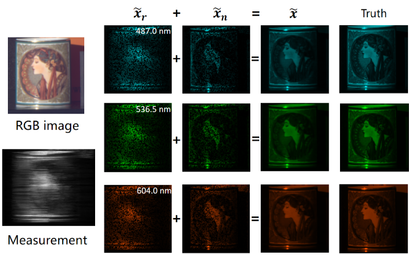
Figure 1: Deep range-null space decomposition for hyperspectral image reconstruction. The picture shows the main reconstruction ideas of the Range-Null Space Decomposition (RND) method. RND-SCI respectively reconstructs the data-fidelity (range-space) term $\tilde{\boldsymbol{x}}_{r}$ and the regularization (null-space) term $\tilde{\boldsymbol{x}}_{n}$. By adding the two parts, we get the reconstructed images $\tilde{\boldsymbol{x}}$.

Compared to RGB images, hyperspectral images (HSIs) consist of numerous discrete bands to convey more spectral information beyond the visible. Therefore, they are a formidable tool in the realm of remote sensing [18], and visual recognition [13, 34]. However, capturing hyperspectral images at high spatial and spectral resolution at a fast speed is challenging with traditional imaging systems. To alleviate the problem, the coded aperture snapshot spectral imaging (CASSI) system [29] (Figure 3), based on compressed sensing technology [8], has been proposed and developed. The system modulates the 3D HSI signals via a coded aperture and compresses it to a 2D measurement. The main challenge in compressive spectral imaging is to design a reliable and fast algorithm to recover HSIs from a 2D measurement.

Traditional model-based methods [32, 15, 17, 37, 15] attempt to construct a series of hand-crafted features and regularization by analyzing the imaging formation. However, the methods need to tune parameters manually and the generalization suffers from model capacity. One of the simple modeling approaches, an end-to-end method [25, 23, 11, 3], formulates the HSI reconstruction as a regression problem, which can achieve state-of-the-art reconstruction results thanks to the deep neural networks. The disregard for the priors and principles of CASSI systems in those methods hinders their adaptability to diverse real-world scenarios. Also, this kind of method loses flexibility and interpretability between spatial precision and speed in different scenarios.

To address the aforementioned challenges, deep unfolding methods [5, 31, 22, 20] offer a promising approach to combine the principle of CASSI signal encoding to design an HSI decoder network. A common practice in these methods is to formulate the reconstruction from a bayesian perspective:

$$\tilde{\boldsymbol{x}}=\mathop{\arg\min}\limits_{\boldsymbol{x}}\left\|\boldsymbol{y}-\mathbf{\Phi}\boldsymbol{x}\right\|^{2}_{2}+\lambda R(\boldsymbol{x}).$$ (1)

The first data-fidelity term $\left\|\boldsymbol{y}-\mathbf{\Phi}\boldsymbol{x}\right\|^{2}_{2}$ optimizes data consistency, ensuring that the reconstructed results conform to the CASSI system forward process. While the second image-prior term $\lambda R(\boldsymbol{x})$ regularizes the reconstructed result with prior knowledge of HSI distribution. Compared to previous methods, they have made great progress in terms of interpretability and model flexibility. However, Eq.(1) is a non-convex optimization problem which makes it difficult to design a convergent algorithm. Moreover, it’s hard to balance data consistency and regularization for a favorable reconstruction.

In this work, we apply the Range-Null space decomposition to the HSI reconstruction. It offers a new perspective to handle data and regularization terms. The data consistency is only determined by the range-space contents and can be calculated without data-driven learning. Hence, the key problem turns to finding a proper null-space solution that makes the reconstruction performance satisfy HSI real scene distribution. Furthermore, we improve the SAUNet [30] based on Range-Null space decomposition and achieve better reconstruction accuracy with faster reconstruction speed than other real-time HSI reconstruction systems. It can process 91 measurements per second at Tesla V100, approximately doubling the speed of CST-S [4]. In summary, our main contributions are
(1) We apply the Range-Null Space Decomposition method and design a novel framework named RND-SCI, for HSI reconstruction.
(2) Thanks to the flexibility of RND-SCI, different strategies like training from scratch, fine-tuning and Plug-and-Play (PnP) used RND-SCI consistently lead to improved performance in four different HSI algorithms.
(3) Based on the RND-SCI, we propose an extremely fast HSI reconstruction network, RND-SAUNet.
(4) We launch a comprehensive comparison between RND-SAUNet and other different fast HSI reconstruction methods.

2 Related Work

2.1 Compressive Spectral Image Reconstruction

Existing works tackle the ill-posed inverse problems from different perspectives. Traditional methods [15, 17, 37, 15, 27] rely on hand-crafted image priors, e.g. total variation (TV) [37], low-rank [17], and sparsity [29]. However, these methods generally have limited performance and sometimes suffer from long-time consumption.

End-to-end methods [4, 3, 24, 11] can leverage the advantages of neural networks to improve the representation ability. Recently, owing to convolutional neural network limits of long-range dependencies, the transformer architecture has great attention and can recover the images that match the real scenes. However, the methods have little literal theoretical proven [38] and lack the flexibility to balance between the reconstruction precision and speed in real-world usage.

Deep unfolding methods [5, 31, 22, 20, 12], different from the above methods, employ deep neural network as a denoising model in an optimization solver, such as ADMM [2], HQS [9], PGD [1], etc. The methods effectively boost the flexibility and interpretability of the principle of CASSI. However, it is difficult to design a non-convex optimization framework and ensure its convergence and the interpretation of such methods is still lack.

2.2 Range-Null Space Decomposition for inverse imaging

Schwab et al. [26] proposes the method for solving inverse problems and analyzes the rate of convergence. Chen et al. [6] analytically decomposes the reconstruction result into range-space and null-space then fit them respectively. Morteza et al. [21] apply the theory to MRI with generative adversarial neural network (GAN) and achieve great performance. Wang et al. [33] reveal a concise and fast super-resolution network based on the range-null space decomposition framework.

However, as for hyperspectral image reconstruction, the sensing matrix $\boldsymbol{\Phi}$ is a fat and sparse matrix, which leads to solving the pseudo-inverse difficulty. In this paper, we propose a simple and efficient approach according to the properties of the matrix, by conducting several matrix dot product operations to solve pseudo-inverse of the sensing matrix.

3 Method

3.1 Preliminaries

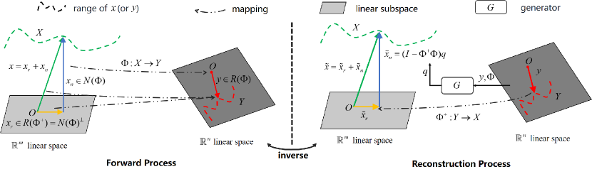
Figure 2: The schematic diagram of Range-Null Space Decomposition. According to the forward process $\boldsymbol{y}=\mathbf{\Phi}\boldsymbol{x}$, the $\mathbb{R}^{m}$ linear space can be uniquely decomposed into two orthogonal subspaces, range space and null space. During the reconstruction process, the range-space reconstructed object is constructed by the pseudo-inverse matrix $\mathbf{\Phi}^{\dagger}$ corresponding to $\mathbf{\Phi}$. While the other object is to first generate a $\boldsymbol{q}$ satisfying the regularization constraint through the conditional generative network and then obtained by the null space projection operator $\boldsymbol{I}-\mathbf{\Phi}^{\dagger}\mathbf{\Phi}$.

3.1.1 CASSI System

A concise spectral image compression pipeline of the CASSI System is shown in Figure 3. The spectral information is modulated by a pre-defined coded aperture mask $\boldsymbol{M}^{*}$ to modulate $\boldsymbol{F}$ and then dispersed by a dispersive prism. Finally, the signals are detected by the detector. Mathematically, we denote $\boldsymbol{M}^{*}\in\mathbb{R}^{H\times W}$ as coded aperture and $\boldsymbol{F}\in\mathbb{R}^{H\times W\times N_{\lambda}}$ as original 3D HSI cube. To simplify, we denote $\boldsymbol{M}\in\mathbb{R}^{H\times(W+d(N_{\lambda}-1))\times N_{\lambda}}$ and $\boldsymbol{F^{\prime\prime}}\in\mathbb{R}^{H\times(W+d(N_{\lambda}-1))\times N_{\lambda}}$ as 3D shifted version of mask $\boldsymbol{M}^{*}$ and 3D HSI cube $\boldsymbol{F}$, where $d$ represents the shifting step. Their relationship is as follows:

$$\boldsymbol{M}(u,v,n_{\lambda})=\boldsymbol{M}^{*}(x,y+d(\lambda_{n}-\lambda_{c}))$$ (2)

$$\boldsymbol{F^{\prime\prime}}(u,v,n_{\lambda})=\boldsymbol{F}(x,y+d(\lambda_{n}-\lambda_{c}),n_{\lambda})$$ (3)

where $(u,v)$ indicates the position on the detector plane coordinate system. $\lambda_{n}$ represents the wavelength of the $n_{\lambda}$-th spectral channel, and $\lambda_{c}$ is the base wavelength that does not shift after passing a dispersive prism. So the measurement $\boldsymbol{Y}$ is formulated as

$$\boldsymbol{Y}=\sum_{n_{\lambda}=1}^{N_{\lambda}}\boldsymbol{F^{\prime\prime}}(:,:,n_{\lambda})\odot\boldsymbol{M}(:,:,n_{\lambda})$$ (4)

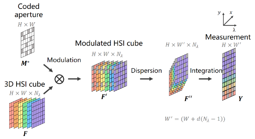
Figure 3: Illustration of the Coded Aperture Snapshot Spectral Imaging (CASSI) system. HSIs are handled by modulation, dispersion, and integration operations to obtain the 2D measurements.

Vectorization.

Let $\mathrm{vec}(\cdot)$ represent the matrix vectorization, i.e., concatenates all the columns of a matrix as a single vector. Define $\boldsymbol{y}=\mathrm{vec}(\boldsymbol{Y})\in\mathbb{R}^{n}$ where $n=H(W+d(N_{\lambda}-1))$. As for original 3D HSI cube, we denote the $\boldsymbol{x}_{n_{\lambda}}=\mathrm{vec}(\boldsymbol{F^{\prime\prime}}(:,:,n_{\lambda}))$. So the vector $\boldsymbol{x}$ is

$$\boldsymbol{x}=\mathrm{vec}([\boldsymbol{x}_{1},\boldsymbol{x}_{2},...,\boldsymbol{x}_{N_{\lambda}}])\in\mathbb{R}^{n{N_{\lambda}}}.$$ (5)

Similar to above steps, as shown in Figure 4, we denote the sensing matrix $\mathbf{\Phi}\in R^{n\times nN_{\lambda}}$ as

$$\mathbf{\Phi}=[\mathbf{\Phi}_{1},\mathbf{\Phi}_{2},...,\mathbf{\Phi}_{N_{\lambda}}],$$ (6)

where $\mathbf{\Phi}=\mathrm{diag}(\mathrm{vec}(\mathrm{\boldsymbol{M}(:,:,n_{\lambda})))}$. The vectorized version of Eq.(4) is rewritten as

$$\boldsymbol{y}=\mathbf{\Phi}\boldsymbol{x}.$$ (7)

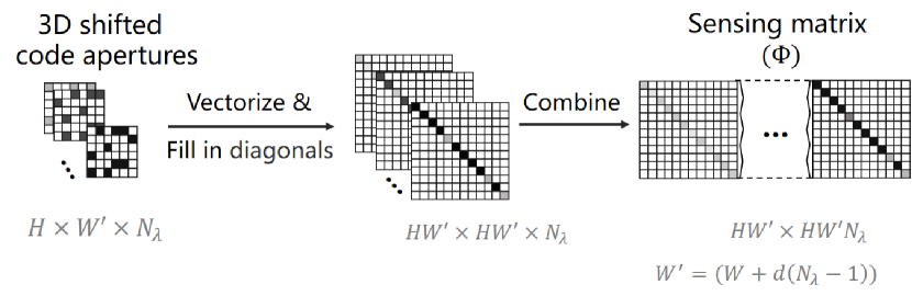
Figure 4: The transition process from coded aperture to sensing matrix. To generate the sensing matrix, the 3D shifted coded aperture is first vectorized and filled in each diagonal of zero matrices and then combine with the number of spectral band diagonal matrices.

3.1.2 Range-Null Space Decomposition

Figure 2 shows the main idea of the Range-Null space decomposition. A linear imaging system can be described as Eq. 7, where $\boldsymbol{y}\in\mathbb{R}^{n}$, $\boldsymbol{x}\in\mathbb{R}^{m}$ and $\mathbf{\Phi}:\mathbb{R}^{m}\rightarrow\mathbb{R}^{n}$ is a mapping between a linear spaces $\mathbb{R}^{n}$ and $\mathbb{R}^{m}$. We define the null space of the $\mathbf{\Phi}$ as $N(\mathbf{\Phi})$, which satisfies

$$N(\mathbf{\Phi})=\{\boldsymbol{x}_{n}|\mathbf{\Phi}\boldsymbol{x}_{n}=0\}$$ (8)

And we treat the vector $\boldsymbol{x}$ as two parts: $\boldsymbol{x}_{r}$ and $\boldsymbol{x}_{n}$, where $\boldsymbol{x}_{n}{\in}N(\mathbf{\Phi})$ and $\boldsymbol{x}_{r}{\in}N(\mathbf{\Phi})^{\perp}$. And $N(\cdot)^{\perp}$ indicates the subspace perpendicular to $N(\cdot)$, i.e. the range subspace. The projection operation maps the two vectors to $\boldsymbol{y}$ and zero vector in $\mathbb{R}^{m}$ space, and the sum of the mapping vectors exactly equals $\boldsymbol{y}$.

During the reconstruction process, we note the pseudo-inverse of $\mathbf{\Phi}$ as $\mathbf{\Phi}^{\dagger}$. We can prove that the general solution of the Eq. 7 is

$$\tilde{\boldsymbol{x}}=\mathbf{\Phi}^{\dagger}\boldsymbol{y}+(\boldsymbol{I}-\mathbf{\Phi}^{\dagger}\mathbf{\Phi})\boldsymbol{q},$$ (9)

where $\boldsymbol{I}$ is a unit matrix and $\boldsymbol{q}$ is a random vector in $\mathbb{R}^{m}$. Since $\mathbf{\Phi}\mathbf{\Phi}^{\dagger}\mathbf{\Phi}\equiv\mathbf{\Phi}$, we consider $\mathbf{\Phi}\mathbf{\Phi}^{\dagger}\mathbf{\Phi}$ as the project operator that maps samples into the range space of $\mathbf{\Phi}$. Furthermore, $\mathbf{\Phi}(\boldsymbol{I}-\mathbf{\Phi}^{\dagger}\mathbf{\Phi})\equiv\boldsymbol{0}$ so that $(\boldsymbol{I}-\mathbf{\Phi}^{\dagger}\mathbf{\Phi})$ can be seen as the operator that maps samples into null-space of $\mathbf{\Phi}$.

Based on above, we use $\tilde{\boldsymbol{x}}_{r}=\mathbf{\Phi}^{\dagger}\boldsymbol{y}$ to represent the reconstructed range-space results while $\tilde{\boldsymbol{x}}_{n}=(\boldsymbol{I}-\mathbf{\Phi}^{\dagger}\mathbf{\Phi})\boldsymbol{q}$ to represent the null-space results. We can employ a conditional generative network to produce an approximate and satisfactory $\boldsymbol{q}$ via $(Y,\mathbf{\Phi})$. Because $\tilde{\boldsymbol{x}_{r}}$ is determined, this pipeline is essential to design a conditional generative network to learn a mapping from $(Y,\mathbf{\Phi})$ to the null space of $X$.

3.2 Overall Architecture

Our framework is shown as Figure 5. Based on the theory of range-null space decomposition, we design the range-space reconstruction module and the null-space reconstruction module to produce the range-space value $\tilde{\boldsymbol{x}}_{r}$ and null-space value $\tilde{\boldsymbol{x}}_{n}$ respectively. The final output $\tilde{\boldsymbol{x}}$ is the dot sum of the two reconstructed images.

The range-space reconstruction module consists of a matrix linear operation $\mathbf{\Phi}^{\dagger}\boldsymbol{y}$, where $\mathbf{\Phi}^{\dagger}$ is the pseudo-inverse of the sensing matrix $\mathbf{\Phi}$ (in Figure 4). The purpose of this module is to guarantee that the reconstruction results are consistent with the degradation process, i.e. $\tilde{\boldsymbol{x}}_{r}$ is one of the solutions of Eq. 7. While the null-space reconstruction module needs a conditional generative neural network to produce an eligible vector $\boldsymbol{q}$ according to the HSI prior constraints. In order to make the final results meet the requirements of data consistency and regularization, the vector $\boldsymbol{q}$ is left multiplied by a null space projection matrix to project $\boldsymbol{q}$ into the null space of $\mathbf{\Phi}$ and acquire $\tilde{\boldsymbol{x}}_{n}$. According to the properties of $\boldsymbol{I}-\mathbf{\Phi}^{\dagger}\mathbf{\Phi}$, the reconstruction target of the neural network should be

$$\boldsymbol{q}=k\boldsymbol{x}_{r}+\boldsymbol{x}_{n},$$ (10)

where $k$ is an arbitrary real number. When $k$ is set to 1, the output of the conditional generative neural network is $\tilde{\boldsymbol{x}}$. Therefore, each existing compressive spectral reconstruction network which is viewed as a conditional generative neural network can insert the RND framework.

So the key problem is how to solve the pseudo-inverse of $\boldsymbol{\Phi}$ to solve the range-space term. It is common to use singular value decomposition(SVD) [16] to compute the analytical solution, that is

$$\boldsymbol{\Phi}=\mathbf{U}\mathbf{\Sigma}\mathbf{V}^{\top},\quad\boldsymbol{\Phi}^{\dagger}=\mathbf{V}\mathbf{\Sigma}^{-1}\mathbf{U}^{\top},$$ (11)

where $\mathbf{U}$ and $\mathbf{V}$ are orthogonal matrices and $\mathbf{\Sigma}$ is a diagonal matrix with eigenvalues as its diagonal elements. However, it is hard to compute directly on account of the sparse and fat $\boldsymbol{\Phi}$. For example, $H$ = 256, $W$ = 256, $N_{\lambda}$ = 28 and store the matrix $\boldsymbol{\Phi}$ as 32 bit float-point number, it takes about 656 GB memory storage. However, under the same conditions, the 3D-shifted coded aperture (left in Figure 4) takes only about 8.4 MB memory storage. A natural idea is to simplify this pseudo-inverse with the help of the CASSI principle.

Figure 5: RND-SCI Framework. The RND-SCI Framework consists of two modules, the range-space reconstruction module(the blue part) and the null-space reconstruction module. The two modules respectively reconstruct the range-space target and null-space target. Finally, the solution target is obtained by adding the reconstruction contents of modules.

As shown in Figure 4, it is worth noting that the special structure of the sensing matrix $\boldsymbol{\Phi}$ will lead to $\boldsymbol{\Phi}\boldsymbol{\Phi}^{\top}$ is a diagonal matrix and the each of the diagonal elements is the sum of the squares of the 3D shifted coded aperture along the spectral band dimension, that is

$$\boldsymbol{\Phi}\boldsymbol{\Phi}^{\top}(u+vH,u+vH)=\sum^{N_{\lambda}}_{n_{\lambda}=1}\boldsymbol{M}^{2}(u,v,n_{\lambda}).$$ (12)

In engineering, it’s easy to guarantee matrix $\boldsymbol{\Phi}\boldsymbol{\Phi}^{\top}$ is a full rank matrix, that is $rank(\boldsymbol{\Phi}\boldsymbol{\Phi}^{\top})=HW$. Due to $rank(\boldsymbol{\Phi}\boldsymbol{\Phi}^{\top})=rank(\boldsymbol{\Phi}^{\top}\boldsymbol{\Phi})=rank(\boldsymbol{\Phi})$, it is easy to prove that matrix $\boldsymbol{\Phi}$ is a row full rank matrix. A simple way to solve the pseudo-inverse of a matrix $\boldsymbol{\Phi}$ is

$$\mathbf{\Phi}^{\dagger}=\mathbf{\Phi}^{\top}(\mathbf{\Phi}\mathbf{\Phi}^{\top})^{-1}.$$ (13)

Note the $(\mathbf{\Phi}\mathbf{\Phi}^{\top})^{-1}=\mathbf{\Sigma}^{-1}$. So we simplify the Eq. 14 as follows:

$$\tilde{\boldsymbol{x}}=\mathbf{\Phi}^{\top}(\mathbf{\Sigma}^{-1}\boldsymbol{y})+[\boldsymbol{q}-\mathbf{\Phi}^{\top}\mathbf{\Sigma}^{-1}(\mathbf{\Phi}\boldsymbol{q})].$$ (14)

Notice that we just need a couple of element-wise computations to solve for $\boldsymbol{x}$ from $\boldsymbol{q}$, $\boldsymbol{\Phi}$ and $\boldsymbol{y}$. Hence, the method for HSI reconstruction is very efficient and accurate when the vector $\boldsymbol{q}$ is reconstructed exactly.

3.3 Fast HSI Reconstruction

In order to maximize the performance and speed up the reconstruction process, we design RND-SAUNet, combining with improved SAUNet [30] and RND.

SAUNet unfolds the ADMM optimization algorithm and incorporates a set of learnable parameters for relaxing the residual terms. Each sub-network comprises a linear layer and a U-shaped denoiser with Transformer-style CNN [10]. Although it can be quite fast and achieve high accuracy performance. However, We are able to make some following adjustments to boost the speed and stability of the network.

Better initialization.

As for the original SAUNet, we first repeat $\boldsymbol{y}$ in spectral dimension. Note the repeated tensor as $Z$. The next 3D shift operation can be formulated as

$$Z_{s}(u,v,c)=\begin{cases}Z(u,v-dc,c),&0\leq v-dc\leq W,\\ 0,&v-dc\leq 0,\end{cases}$$ (15)

where $Z_{s}$ is the tensor $Z$ after the 3D shift operation and c is the index of spectral dimension.

But the shifted operation with zero padding may lack some spectral characteristic information, which leads to generating a poor initialization $z^{0}$. Hence, the poor initialization further increases the burden of the subsequent denoising network.

One improvement (Figure 6) is to use $Z$ as input to produce $z^{0}$. However, the matrix $\Phi$ is shifted based on the following operations. This may lead to confusing interactions between $\Phi$ and affect the performance of the initialization $z^{0}$.

So we finally come up with a new method to input approach to generate initialization. As shown in (c) of Figure 6, after the 3D roll for the tensor $Z$, the rolled tensor $Z_{r}$ can be represented as

$$Z_{r}(u,v,c)=Z(u,(v-dc+W)\%W,c),$$ (16)

where the operation $\%$ is a modulo operation.

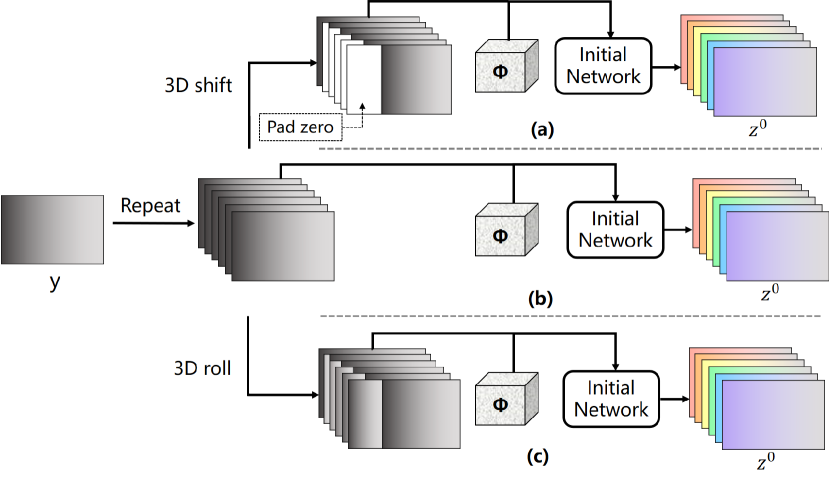
Figure 6: Three kinds of initial network design. (a) for original SAUNet, (b) and (c) are more stable initial network designs. (b) is that direct using repeated y as initial network input, while (a) and (c) generate input via the two different operations, 3D shift, and 3D roll.

Cropped input into denoiser.

For a fast reconstruction, as shown in Figure 7, we depart from the original denoiser input as HSIs with noise (the colored part) and the shifted part from HSIs (the white part). One intuitive idea is to feed noisy HSI signals into the network. This method not only can speed up the network and reduce the computational complexity but also does not cause a significant reduction in accuracy.

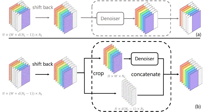
Figure 7: Crop the denoiser input.

Algorithms	Params	GFLOPs	S1	S2	S3	S4	S5	S6	S7	S8	S9	S10	Avg
DGSMP [12]	3.76M	646.65	33.26 0.915	32.09 0.898	33.06 0.925	40.54 0.964	28.86 0.882	33.08 0.937	30.74 0.886	31.55 0.923	31.66 0.911	31.44 0.925	32.63 0.917
TSA-Net [23]	44.25M	110.06	33.48 0.919	32.70 0.900	34.63 0.942	41.26 0.973	30.90 0.921	32.33 0.934	31.42 0.902	30.62 0.924	32.65 0.926	29.90 0.896	32.99 0.924
GAP-Net [22]	4.27M	78.58	33.74 0.911	33.26 0.900	34.28 0.929	41.03 0.967	31.44 0.919	32.40 0.925	32.27 0.902	30.46 0.905	33.51 0.915	30.24 0.895	33.26 0.917
ADMM-Net [20]	4.27M	78.58	34.12 0.918	33.62 0.902	35.04 0.931	41.15 0.966	31.82 0.922	32.54 0.924	32.42 0.896	30.74 0.907	33.75 0.915	30.68 0.895	33.58 0.918
MST-S [3]	0.93M	12.96	34.71 0.930	34.45 0.925	35.32 0.943	41.50 0.967	31.90 0.933	33.85 0.943	32.69 0.911	31.69 0.933	34.67 0.939	31.82 0.926	34.26 0.935
CST-S [4]	1.20M	11.67	34.78 0.930	34.81 0.931	35.42 0.944	41.84 0.967	32.29 0.939	34.49 0.949	33.47 0.922	32.89 0.945	34.96 0.944	32.14 0.932	34.71 0.940
HDNet [11]	2.37M	157.76	35.14 0.935	35.67 0.940	36.03 0.943	42.30 0.969	32.69 0.946	34.46 0.952	33.67 0.926	32.48 0.941	34.89 0.942	32.38 0.937	34.97 0.943
SAUNet-1stg [30]	0.78M	9.52	34.66 0.936	34.78 0.933	36.74 0.955	43.33 0.979	32.14 0.941	34.28 0.952	33.29 0.927	32.18 0.947	35.24 0.950	31.79 0.936	34.84 0.946
RND-SAUNet(Ours)	0.78M	7.84	34.91 0.937	35.19 0.933	37.12 0.955	42.28 0.971	32.34 0.941	34.44 0.952	33.43 0.926	32.66 0.944	35.56 0.948	32.07 0.936	35.00 0.944

Table 1: Comparisons between RND-SAUNet and SOTA low time-consuming methods on 10 simulation scenes (S1$\sim$S10). Params, FLOPS, PSNR (upper entry in each cell), and SSIM (lower entry in each cell) are reported.

4 Experiments

4.1 Experiments Setting

We follow TSA-Net [23] to adopt 28 wavelengths from 450nm to 650nm derived by spectral interpolation for simulation HSI reconstruction experiments.

Datasets

In our experiments, we choose two publicly available datasets, namely CAVE [36] and KAIST [7], and to ensure a fair comparison, we utilize a mask of size $256\times 256$, identical to that of TSA-Net. And the test dataset consists of 10 scenes from KAIST, while the others are used for training.

Implementation

We implement our model in PyTorch. All models are trained with Adam optimizer [14] ($\beta_{1}=0.9$ and $\beta_{2}=0.999$) for 300 epochs. The learning rate is set to $4\times 10^{-4}$ at the beginning and is halved every 50 epochs during the training procedure. We randomly crop patches with the spatial size of $256\times 256$ and $660\times 660$ from 3D HSI cubes as training samples for simulation and real experiments. Following TSA-Net [23], the shifting step $d$ in dispersion is set to 2 and the batch size is 5. We set reconstructed channel $C=N_{\lambda}=28$. Data augmentation is made of random flipping and rotation. The training cost function is to follow the design of the original model.

Finally, we adopt PSNR and SSIM for quantitative comparison as reference image quality assessment metrics.

Model	TSA-Net	DGSMP	GAP-Net	ADMM-Net	MST-S	CST-S	HDNet	SAUNet-1stg	RND-SAUNet(Ours)
Training Hours	28.5	148.4	48.8	48.8	48.6	17.5	34.7	14.3	9.6
Inference FPS	32.8	8.0	19.0	18.6	23.2	45.3	44.8	14.3	91.0

Table 2: Comparisons between RND-SAUNet and 8 SOTA low time-consuming methods with their variants in training GPU hours and inference speed at a Tesla v100 GPU. We record the forward and backward time of each model training in a GPU for 300 epochs at batch-size=5 as training hours.

4.2 Reconstruction Results

Table 1 compares the Params, FLOPs, PSNR, and SSIM of RND-SAUNet with other 8 SOTA low time-consuming methods. Our method RND-SAUNet surpasses other methods in both GFLOPs, params, and average PSNR/SSIM. And Table 2 compares training time and test inference FPS of RND-SAUNet with other 8 SOTA low time-consuming methods in a Tesla V100 GPU. We re-train all models for 300 epochs with the toolbox of MST [3] at 5 batch size. For more efficient computation, we use CUDA programming to optimize the 3D shift operations. RND-SAUNet sets new state-of-the-art inference and training speed scores on the simulation datasets. Figure 8 depicts the simulation HSI reconstruction comparisons between our RND-SAUNet and other SOTA methods on Scene 2 with 4 (out of 28) spectral channels. RND-SAUNet has more similar spectral density curves compared to other counterparts.

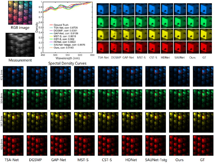
Figure 8: Reconstructed simulation HSI comparisons of Scene 2 with 4 out of 28 spectral channels.The top-left shows the target scene RGB image and 2D measurement. The top-middle shows the spectral curves corresponding to the red box of the RGB image. The top-right depicts the enlarged patches corresponding to the red boxes in the bottom HSIs. Zoom in for a better view.

4.3 Ablation Study for RND-SAUNet

We conduct a break-down ablation experiment to investigate the effect of each component towards higher performance or a fast speed. The results are listed in Table 3 and Table 4.

crop	init	RND	PSNR	SSIM	params (M)	GFLOPs
			34.84	0.946	0.78M	9.52
✓			34.63	0.943	0.78M	7.83
	✓		34.86	0.946	0.78M	9.52
✓	✓		34.77	0.946	0.78M	7.84
✓		✓	34.75	0.942	0.78M	7.83
	✓	✓	35.08	0.945	0.78M	9.52
✓	✓	✓	35.00	0.944	0.78M	7.84

Table 3: Ablation study of crop, initialization and range-null decomposition.

Influence of good initialization.

We set three baselines, the original SAUNet-1stg, the one with cropping operation, and the RND-SAUNet without initialization improvement in Table 3. We can find the results increase by 0.02dB, 0.14dB, and 0.25 dB. It demonstrates that a good initialization is conducive to more accurate reconstruction performance. In order to further explore the impact of different initialization methods on the reconstruction results, we employ the different initial network inputs in SAUNet with cropping denoiser input and RND-SAUNet. From Table 4, we can observe approach c gets the best PSNR and SSIM in two different situations. This verifies that the 3D roll operation is more efficient for generating the initial HSIs that retain more valid information.

Influence of cropping operation.

The baselines are the original SAUNet-1stg, the one with the initial approach c in Figure 6, and the one with all improvements except cropping. When we crop each denoiser input, although the PSNR metrics are lost by 0.21, 0.09 dB, and 0.08 dB, the computation overheads both decrease by 1.69 GFLOPs. This shows that crop operation can save some calculations, however, when high reconstruction accuracy is required, the information shifted from HSI is the same important.

Influence of RND-SCI Framework.

In Table, we employ the RND-SCI framework into SAUNet with cropping denoiser input, SAUNet at an initial approach c, and the one with both above. The performances are better than 0.12dB, 0.22dB, and 0.23 dB, and without much increase in computation. It illustrates the effectiveness of the RND-SCI framework SAUNet.

init	RND	PSNR	SSIM
a		34.63	0.943
b		34.76	0.944
c		34.77	0.946
a	✓	34.75	0.942
b	✓	34.87	0.942
c	✓	35.00	0.944

Table 4: Ablation study of different initialization strategies for RND-SAUNet and SAUNet with cropping denoiser input.

	original		mask1		mask2
method	PSNR	SSIM	PSNR	SSIM	PSNR	SSIM
TSA-Net [23]	32.99	0.923	32.68	0.921	32.91	0.922
MST-S [3]	34.26	0.935	34.30	0.938	34.43	0.939
CST-S [4]	34.71	0.940	34.63	0.945	34.67	0.944
RND-MST-S	34.88	0.942	34.66	0.940	34.83	0.942
RND-CST-S	34.86	0.943	34.72	0.941	34.79	0.942
RND-SAUNet	35.00	0.944	34.82	0.944	34.92	0.943

Table 5: Robustness test with different modulated masks.

4.4 Generalization for Modulated Mask

In this part, we want to explore the different models for the random modulated mask. We change the mask by randomly cropping it with size $256\times 256$ from the real mask of size $660\times 660$ to evaluate the flexibility of the RND-SCI framework and RND-SAUNet for different signal modulations. The results are reported in Table 5. Compared with the other models, the model with RND-SCI can achieve more accurate reconstruction performance. These results suggest that the RND-SCI framework is more robust and flexible to improve the model’s HSI reconstruction.

method	RND	PSNR	SSIM
MST-S		34.26	0.940
MST-S	✓	34.88	0.942
MST-M		34.94	0.943
MST-M	✓	35.36	0.949
CST-S		34.71	0.940
CST-S	✓	34.86	0.943
CST-M		35.31	0.947
CST-M	✓	35.42	0.948
SAUNet		34.84	0.946
SAUNet	✓	35.00	0.944

Table 6: Ablation study of different HSI methods applying Range-Null space decomposition.

	original		finetune + RND		PnP RND
method	PSNR	SSIM	PSNR	SSIM	PSNR	SSIM
TSA-Net [23]	32.99	0.923	33.12	0.922	33.09	0.921
MST-S [3]	34.26	0.935	34.63	0.940	34.43	0.937
MST-M [3]	34.94	0.943	35.32	0.950	35.04	0.947
CST-S [4]	34.71	0.940	34.85	0.943	34.84	0.943
CST-M [4]	35.31	0.947	35.42	0.950	35.42	0.950

Table 7: Fine-tuning and Plug-and Play with RND.

4.5 Generalization for RND-SCI Framework

Our RND-SCI framework is a generic HSI reconstruction method and can be used in applications other than different types of methods and size models. To prove it, we apply RND-SCI to MST-S, MST-M, CST-S, CST-M, and SAUNet and train them from scratch. As shown in Table 6. All methods model has improved at least 0.11 dB. It displays the generalization of RND-SCI for the HSI reconstruction task.

Moreover, fine-tune existing models with it or insert a pre-trained model directly into the RND-SCI framework to get better results. We finetune TSA-Net, MST-S, MST-M, CST-S, and CST-M at the beginning learning rate of $1\times 10^{-5}$, warm-up about 1000 steps, and for 50 epochs. The results are displayed in Table 7 indicates the diversity of RND-SCI implementations and also shows the potential of this decomposition method to solve the compressive spectral imaging inverse problem.

5 Conclusion and Future Work

In this paper, we proposed a simple and flexible framework, RND-SCI, for snapshot compressive imaging. The proposed framework is based on the theory of the range-null space decomposition, which provides a new perspective on modeling data consistency (range-space term) and regularization (null-space term). The data-fidelity term can be obtained directly by a linear projection operation without learning. While the image prior term generates a solution that conforms to a real constraint through a conditional generation network, and then passes through a null-space projection operation. Finally, the two components are aggregated to derive the ultimate reconstruction outcome.

To achieve fast and simple reconstruction, we derive a simple projection operation approach inspired by the principles of CASSI and apply it to an enhanced version of SAUNet, achieving the 91 frames per second reconstruction speed and favorable accuracy. Moreover, we launch extensive experiments to investigate the framework robustness of the modulated mask, different neural networks, and different implementations. Compared with the original model methods, there is evident promotion.

In further work, we hope to take the unified method to extend more similar problems about the hyperspectral image field task, such as hyperspectral image restoration and hyperspectral image super-resolution, to improve the model performance and interpretation, and even develop a unified architecture to solve the set of similar hyperspectral imaging inverse problems on the basis of the theory.

Appendix

The supplementary material is organized as follows:

• Section A: real HSI reconstruction for RND-SAUNet.

• Section B: more comparisons for RND-SAUNet.

• Section C: parameter analysis for RND-SAUNet.

• Section D: limitations and social impacts.

Appendix A Real HSI Reconstruction for RND-SAUNet

Implementation.

Following TSA-Net settings. we re-train RND-SAUNet with a real mask on the KAIST and CAVE datasets jointly, which our paper has mentioned, while the training samples are also injected with 11-bit shot noise for simulating the real imaging situations.

Real HSI reconstruction for RND-SAUNet.

Figure 9 and Figure 10 show the visual comparisons between our RND-SAUNet and other less time-consuming methods. although our methods can reconstruct the structure of the scene and some details, suffering from the lack of design in imaging noise, the simple image plus operator can not remove the noise, which results in the HSI reconstruction having some hollows.

Appendix B More Comparisons for RND-SAUNet

Training memory.

Table 8 shows the memory required to train the HSI algorithms. For a fair comparison, We set the batch size as 5 for all algorithms, except DGSMP for batch size as 2. Compared to other methods, RND-SAUNet is memory-friendly, which only costs 6.50 GB of memory during training.

Model	TSA-Net	DGSMP	GAP-Net	ADMM-Net	MST-S	CST-S	HDNet	SAUNet-1stg	RND-SAUNet(Ours)
Training Memory(GB)	11.20	13.79	8.17	8.78	9.19	8.14	7.83	7.48	6.50

Table 8: Comparisons between RND-SAUNet and 8 SOTA less time-consuming method in training memory. We set the batch-size as 5 for all algorithms, expect DGSMP for 2.

Other visual comparisons.

Figure 11 and 12 show the reconstructed simulation HSI comparisons of Scene 5, 7, and 10 with 4 out of 28 spectral channels. Compared to Seven less time-consuming algorithms. Please zoom in for a better view. As can be seen from the reconstructed HSI, our method RND-SAUNet can recover high-frequency HSI contents and structural textures, resulting in producing perceptually-pleasing images.

Appendix C Parameter Analysis for RND-SAUNet

To further investigate the influence of the changes of the initial network and cropping operator, we compare the two hyper-parameters value $\alpha$ and $\beta$ between the SAUNet-1stg and RND-SAUNet. As shown in the table 9, the $\alpha$, the value of $\alpha$ increases while $\beta$ decreases, which may indicate a better recovery of the image via these improvements.

Method	$\alpha$	$\beta$
SAUNet-1stg	325.08	$0.6\times 10^{-}3$
RND-SAUNet	629.91	$1.0\times 10^{-}6$

Table 9: The hyper-parameter of SAUNet-1stg and RND-SAUNet.

Appendix D Limitations and Social Impacts.

There remain some limitations that deserve further study.

• Though RND-SAUNet achieves the fastest results and gets favorable reconstruction performance among the less time-consuming methods, it is still limited in accuracy compared to the high-precision methods, such as DAUHST.

• RND-SCI needs a certain coded aperture mask. It may lead to the model not adapting to the change in the CASSI system.

• RND-SCI does not design to remove imaging noise of the real scene.

Hyperspectral compressive imaging is one of the core tasks in snapshot compressive imaging (SCI) and has been developed for decades. It has been widely used for object detection [35], medical imaging [19], remote sensing [28], and so on. Our algorithm is aimed to improve the speed of reconstruction over all existing other SOTA methods (RND-SAUNet) and provide a unified and easy-to-implement framework (RND-SCI) for a better reconstruction performance. Until now, HSI reconstruction has had no negative social impact, but our study involves GPU resources for training the models, which will result in $\mathrm{CO_{2}}$ emissions.

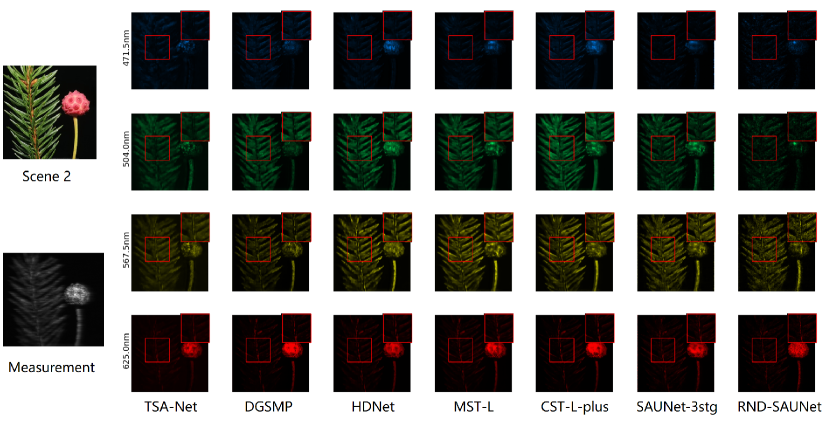
Figure 9: Reconstructed real HSI comparisons on Scene 2 with 4 out of 28 spectral channels. Six SOTA less time-consuming methods and RND-SAUNet are included. Zoom in for a better view.

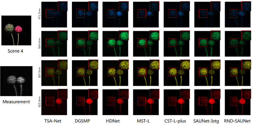
Figure 10: Reconstructed real HSI comparisons on Scene 4 with 4 out of 28 spectral channels. Six SOTA less time-consuming methods and RND-SAUNet are included. Zoom in for a better view.

Figure 11: Reconstructed real HSI comparisons on Scene 5 with 4 out of 28 spectral channels. Seven SOTA less time-consuming methods and RND-SAUNet are included. Zoom in for a better view.

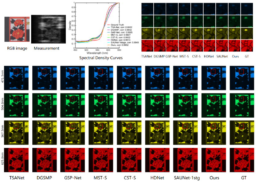
Figure 12: Reconstructed real HSI comparisons on Scene 7 with 4 out of 28 spectral channels. Seven SOTA less time-consuming methods and RND-SAUNet are included. Zoom in for a better view.

References

- [1] Amir Beck and Marc Teboulle. A fast iterative shrinkage-thresholding algorithm for linear inverse problems. In SIIMS, 2009.
- [2] Stephen Boyd, Neal Parikh, Eric Chu, Borja Peleato, Jonathan Eckstein, et al. Distributed optimization and statistical learning via the alternating direction method of multipliers. Found. Trends Mach. Learn., 2011.
- [3] Yuanhao Cai, Jing Lin, Xiaowan Hu, Haoqian Wang, Xin Yuan, Yulun Zhang, Radu Timofte, and Luc Van Gool. Mask-guided spectral-wise transformer for efficient hyperspectral image reconstruction. In CVPR, 2022.
- [4] Yuanhao Cai, Jing Lin, Xiaowan Hu, Haoqian Wang, Xin Yuan, Yulun Zhang, Radu Timofte, and Luc Van Gool. Coarse-to-fine sparse transformer for hyperspectral image reconstruction. In ECCV, 2022.
- [5] Yuanhao Cai, Jing Lin, Haoqian Wang, Xin Yuan, Henghui Ding, Yulun Zhang, Radu Timofte, and Luc Van Gool. Degradation-aware unfolding half-shuffle transformer for spectral compressive imaging. arXiv:2205.10102, 2022.
- [6] Dongdong Chen and Mike E Davies. Deep decomposition learning for inverse imaging problems. In ECCV, 2020.
- [7] Inchang Choi, Daniel S. Jeon, Giljoo Nam, Diego Gutierrez, and Min H. Kim. High-quality hyperspectral reconstruction using a spectral prior. In SIGGRAPH Asia, 2017.
- [8] D.L. Donoho. In Compressed sensing, 2006.
- [9] Ran He, Wei-Shi Zheng, Tieniu Tan, and Zhenan Sun. Half-quadratic-based iterative minimization for robust sparse representation. In TPAMI, 2013.
- [10] Qibin Hou, Cheng-Ze Lu, Ming-Ming Cheng, and Jiashi Feng. Conv2former: A simple transformer-style convnet for visual recognition. arXiv:2211.11943, 2022.
- [11] Xiaowan Hu, Yuanhao Cai, Jing Lin, Haoqian Wang, Xin Yuan, Yulun Zhang, Radu Timofte, and Luc Van Gool. Hdnet: High-resolution dual-domain learning for spectral compressive imaging. In CVPR, 2022.
- [12] Tao Huang, Weisheng Dong, Xin Yuan, Jinjian Wu, and Guangming Shi. Deep gaussian scale mixture prior for spectral compressive imaging. In CVPR, 2021.
- [13] Min H Kim, Todd Alan Harvey, David S Kittle, Holly Rushmeier, Julie Dorsey, Richard O Prum, and David J Brady. 3d imaging spectroscopy for measuring hyperspectral patterns on solid objects. In TOG, 2012.
- [14] Diederik P Kingma and Jimmy Ba. Adam: A method for stochastic optimization. arXiv:1412.6980, 2014.
- [15] David Kittle, Kerkil Choi, Ashwin Wagadarikar, and David J Brady. Multiframe image estimation for coded aperture snapshot spectral imagers. In Applied Optics, 2010.
- [16] Virginia Klema and Alan Laub. The singular value decomposition: Its computation and some applications. In TAC, 1980.
- [17] Yang Liu, Xin Yuan, Jinli Suo, David J Brady, and Qionghai Dai. Rank minimization for snapshot compressive imaging. In TPAMI, 2018.
- [18] Bing Lu, Phuong D Dao, Jiangui Liu, Yuhong He, and Jiali Shang. Recent advances of hyperspectral imaging technology and applications in agriculture. In Remote Sensing, 2020.
- [19] Guolan Lu and Baowei Fei. Medical hyperspectral imaging: a review. In Journal of biomedical optics, 2014.
- [20] Jiawei Ma, Xiao-Yang Liu, Zheng Shou, and Xin Yuan. Deep tensor admm-net for snapshot compressive imaging. In ICCV, 2019.
- [21] Morteza Mardani, Enhao Gong, Joseph Y. Cheng, Shreyas S. Vasanawala, Greg Zaharchuk, Lei Xing, and John M. Pauly. Deep generative adversarial neural networks for compressive sensing mri. In TMI, 2019.
- [22] Ziyi Meng, Shirin Jalali, and Xin Yuan. Gap-net for snapshot compressive imaging. arXiv:2012.08364, 2020.
- [23] Ziyi Meng, Jiawei Ma, and Xin Yuan. End-to-end low cost compressive spectral imaging with spatial-spectral self-attention. In ECCV, 2020.
- [24] Ziyi Meng, Mu Qiao, Jiawei Ma, Zhenming Yu, Kun Xu, and Xin Yuan. Snapshot multispectral endomicroscopy. In Optics Letters, 2020.
- [25] Xin Miao, Xin Yuan, Yunchen Pu, and Vassilis Athitsos. l-net: Reconstruct hyperspectral images from a snapshot measurement. In ICCV, 2019.
- [26] Johannes Schwab, Stephan Antholzer, and Markus Haltmeier. Deep null space learning for inverse problems: convergence analysis and rates. In Inverse Problems, 2019.
- [27] Jin Tan, Yanting Ma, Hoover Rueda, Dror Baron, and Gonzalo R Arce. Compressive hyperspectral imaging via approximate message passing. In JSTSP, 2015.
- [28] Freek D Van der Meer, Harald MA Van der Werff, Frank JA Van Ruitenbeek, Chris A Hecker, Wim H Bakker, Marleen F Noomen, Mark Van Der Meijde, E John M Carranza, J Boudewijn De Smeth, and Tsehaie Woldai. Multi-and hyperspectral geologic remote sensing: A review. In IJAEOG, 2012.
- [29] Ashwin Wagadarikar, Renu John, Rebecca Willett, and David Brady. Single disperser design for coded aperture snapshot spectral imaging. In Applied Optics, 2008.
- [30] Junyu Wang, Shijie Wang, Wenyu Liu, Zengqiang Zheng, and Xinggang Wang. A simple adaptive unfolding network for hyperspectral image reconstruction. arXiv:2301.10208, 2023.
- [31] Lizhi Wang, Chen Sun, Maoqing Zhang, Ying Fu, and Hua Huang. Dnu: Deep non-local unrolling for computational spectral imaging. In CVPR, 2020.
- [32] Lizhi Wang, Zhiwei Xiong, Guangming Shi, Feng Wu, and Wenjun Zeng. Adaptive nonlocal sparse representation for dual-camera compressive hyperspectral imaging. In TPAMI, 2016.
- [33] Yinhuai Wang, Yujie Hu, Jiwen Yu, and Jian Zhang. Gan prior based null-space learning for consistent super-resolution. arXiv:2211.13524, 2022.
- [34] Yang Xu, Zebin Wu, Jun Li, Antonio Plaza, and Zhihui Wei. Anomaly detection in hyperspectral images based on low-rank and sparse representation. In TGRS, 2015.
- [35] Longbin Yan, Min Zhao, Xiuheng Wang, Yuge Zhang, and Jie Chen. Object detection in hyperspectral images. In SPL, 2021.
- [36] Fumihito Yasuma, Tomoo Mitsunaga, Daisuke Iso, and Shree K Nayar. Generalized assorted pixel camera: postcapture control of resolution, dynamic range, and spectrum. In TIP, 2010.
- [37] Xin Yuan. Generalized alternating projection based total variation minimization for compressive sensing. In ICIP, 2016.
- [38] Xin Yuan, David J Brady, and Aggelos K Katsaggelos. Snapshot compressive imaging: Theory, algorithms, and applications. In SPM, 2021.