FedHGN: A Federated Framework for Heterogeneous Graph Neural Networks

Abstract

Heterogeneous graph neural networks (HGNNs) can learn from typed and relational graph data more effectively than conventional GNNs. With larger parameter spaces, HGNNs may require more training data, which is often scarce in real-world applications due to privacy regulations (e.g., GDPR). Federated graph learning (FGL) enables multiple clients to train a GNN collaboratively without sharing their local data. However, existing FGL methods mainly focus on homogeneous GNNs or knowledge graph embeddings; few have considered heterogeneous graphs and HGNNs. In federated heterogeneous graph learning, clients may have private graph schemas. Conventional FL/FGL methods attempting to define a global HGNN model would violate schema privacy. To address these challenges, we propose FedHGN, a novel and general FGL framework for HGNNs. FedHGN adopts schema-weight decoupling to enable schema-agnostic knowledge sharing and employs coefficients alignment to stabilize the training process and improve HGNN performance. With better privacy preservation, FedHGN consistently outperforms local training and conventional FL methods on three widely adopted heterogeneous graph datasets with varying client numbers. The code is available at https://github.com/cynricfu/FedHGN.

1 Introduction

Graph neural networks (GNNs) Defferrard et al. (2016); Kipf and Welling (2017); Hamilton et al. (2017); Velickovic et al. (2018); Zhang et al. (2022a, c) combine graph representation learning and deep learning to handle graph-structured data more effectively than traditional methods Perozzi et al. (2014); Tang et al. (2015); Grover and Leskovec (2016); Zhang et al. (2022b). GNNs have various applications, such as community detection Chen et al. (2019); Jin et al. (2019), recommender systems van den Berg et al. (2017); Ying et al. (2018); Yang et al. (2022); Chen et al. (2022), traffic forecasting Li et al. (2018); Zhang et al. (2018); Yu et al. (2018), and text similarity Ma et al. (2022). However, many real-world graphs are heterogeneous graphs, which have multiple types of nodes and edges. For instance, a financial network may consist of customers, merchants, transactions, and various relationships among them. Therefore, researchers have developed heterogeneous GNNs (HGNNs), such as RGCN Schlichtkrull et al. (2018), to capture the complex semantics in heterogeneous graph structures.

Similar to other deep learning models, GNN performance depends on the size of the training data. If the training data is insufficient, GNNs may overfit and fail to generalize to unseen data. This problem is more severe for HGNNs, which have much larger parameter spaces Schlichtkrull et al. (2018). Moreover, in reality, adequate training data is often unavailable, which hinders HGNN’s performance.

One possible solution to data scarcity is to collect and integrate samples from multiple parties to create a large shared dataset for model training. However, this approach raises serious privacy concerns in many application scenarios, which prevent HGNNs from using training data in a centralized way. For instance, banks and insurance companies may want to collaborate on developing an HGNN for better fraud detection. But their data, such as customer information and transaction records, are highly sensitive. They cannot transmit these data to another place for HGNN training. Therefore, there is a trade-off between data availability and data privacy. HGNNs trained separately at each client (e.g., a financial institution in this case) would perform poorly due to limited training data, while centralized training by aggregating data from all clients is not feasible due to commercial or regulatory reasons (e.g., GDPR). This leads to a question: can we train an HGNN that leverages each client’s training data without violating local data privacy?

Federated learning (FL) is a promising technique to achieve this goal. Instead of sharing private data, FL clients upload model weights to a central server which aggregates them to improve the global model. The collaboratively trained model is expected to outperform the models trained locally at each client. Previous FL frameworks mainly focused on computer vision (CV) and natural language processing (NLP) tasks McMahan et al. (2017); Li et al. (2020, 2022). Federated graph learning (FGL), i.e., FL on graph-structured data, has just emerged in recent years. Some works have explored FGL in homogeneous graphs Zhang et al. (2021); Xie et al. (2021), recommender systems Wu et al. (2021), and knowledge graphs Chen et al. (2021); Peng et al. (2021). However, FL with heterogeneous graphs and HGNNs, which have a great need for collaborative training, has received little attention.

Real-world federated heterogeneous graph learning faces two unique challenges. First, unlike homogeneous graphs, heterogeneous graphs have special metadata called graph schemas. These are meta templates that describe the node types and edge types of the graph. For example, Figure 1 shows a graph schema of a scholar network. The problem is , clients may not want to share the schema information, which is essential to define an HGNN model. The graph schema reveals high-level information about how the graph is constructed, which may be sensitive in some domains, such as pharmaceutical companies and financial institutions.

Second, even if schema sharing is allowed among clients, it is usually difficult to match node/edge types of different graphs with each other, which is crucial for HGNNs to reduce complexity and share knowledge. In a federated system, different clients may use different pipelines to construct their heterogeneous graphs. For instance, one client may label their paper nodes as paper while another may call them article. This matching process may not always have the domain knowledge and human expertise available. Moreover, when a new client joins the federated system, this schema matching process needs to be repeated, and the HGNN may need to be re-defined to include new node/edge types, both of which are undesirable for industrial FL applications.

Motivated by the lack of an FGL framework for HGNNs and the challenges above, we propose FedHGN, a Federated learning framework for HGNNs that preserves schema privacy and avoids schema matching. The key idea of FedHGN is to eliminate the direct correspondence between graph schemas and HGNN model weights. We achieve this by applying schema-weight decoupling to decompose HGNN weights into shareable schema-agnostic basis weights and confidential schema-specific coefficients. To prevent the potential discrepancy between coefficients of the same/similar schemas at different clients, FedHGN employs coefficients alignment to minimize the distance between coefficients of most similar node/edge types. Thus, FedHGN enables collaborative training for better-performing HGNNs without sacrificing schema privacy or necessitating schema matching.

In summary, we make the following main contributions:

• We propose FedHGN, a novel FGL framework that enables collaborative HGNN training among clients with private heterogeneous graphs. To our knowledge, this is the first work for general federated HGNN learning.

• We propose a schema-weight decoupling (SWD) strategy to achieve schema-agnostic knowledge sharing, which preserves schema-level privacy among clients.

• We design a schema coefficients alignment (CA) component via a novel regularization term, which stabilizes FedHGN training and improves HGNN performance.

• We conduct extensive experiments on benchmark datasets with varying numbers of clients for node classification. Results show that FedHGN consistently outperforms local training and conventional FL methods.

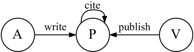
Figure 1: An example graph schema of a scholar network consisting of authors (A), papers (P), and venues (V).

2 Related Work

In this section, we review recent studies related to this work. Section 2.1 introduces graph neural networks (GNNs) and especially heterogeneous GNNs (HGNNs). Section 2.2 introduces conventional federated learning (FL) and recent efforts on federated graph learning (FGL).

2.1 Graph Neural Networks

Graph neural networks (GNNs) are designed to overcome the limitations of shallow graph embedding methods, such as DeepWalk Perozzi et al. (2014) and node2vec Grover and Leskovec (2016). Taking advantage of the neural network architecture, GNNs can leverage node attributes and benefit from various training paradigms of deep learning. The general idea of GNNs is to characterize each node by its own features and its local neighborhood’s information. Following this idea and combined with graph signal processing, spectral-based GNNs like ChebNet Defferrard et al. (2016) and GCN Kipf and Welling (2017) were first developed to perform convolutions in the Fourier domain of a graph. Then, by allowing convolutions in the graph domain, spatial-based GNNs like GraphSAGE Hamilton et al. (2017) and GAT Velickovic et al. (2018) were proposed to improve scalability and generalization ability, with many follow-up studies Xu et al. (2019); Wu et al. (2019).

2.1.1 Heterogeneous GNNs

Conventional GNNs assume homogeneous input graphs with single node/edge types. However, real-world graphs are usually heterogeneous, having multiple node/edge types. To capture complex structural and semantic heterogeneity in these graphs, researchers proposed heterogeneous GNNs (HGNNs). As an early attempt, RGCN Schlichtkrull et al. (2018) aggregates neighborhoods using relation-specific weights. Many other HGNNs follow similar ideas to project and aggregate neighborhoods based on node/edge types, including HetGNN Zhang et al. (2019), HGT Hu et al. (2020), Simple-HGN Lv et al. (2021), etc. Another line of research considers meta-paths to capture complex high-order relationships between nodes, such as HAN Wang et al. (2019b), MAGNN Fu et al. (2020), and GTN Yun et al. (2019).

Although many HGNNs claim to have good performance in real-world applications, none have considered the federated setting with privacy concerns across clients. They simply assume a centralized setting with all data readily available. With privacy restrictions, HGNNs trained with limited local data could suffer from degraded performance and biased predictions. Our proposed FedHGN offers a feasible way to collaboratively train better-performing HGNNs among multiple clients without sharing local graph data and graph schemas.

2.2 Federated Learning

Federated learning (FL) is a machine learning setting for collaborative cross-client model training without sharing raw data Zhang and Zhu (2020); Zhang et al. (2023). Instead of gathering data to a central server, FL keeps data localized on each client and only shares model weights or gradients. Multiple FL algorithms have been proposed for regular data in Euclidean space, such as FedAvg McMahan et al. (2017), FedProx Li et al. (2020), and SCAFFOLD Karimireddy et al. (2020). These FL algorithms are applied in CV and NLP, where data samples are naturally isolated from each other. But for graphs, especially in node-level and link-level tasks, nodes and edges as data samples are associated with each other. Naively migrating conventional FL frameworks might not bring optimal results for graph data.

2.2.1 Federated Graph Learning

Recently, some researchers have proposed FL methods for graphs, which are coined as federated graph learning (FGL). GCFL Xie et al. (2021) employs a client clustering mechanism to reduce data heterogeneity in federated graph classification. FedSage Wu et al. (2021) generates missing neighbors to mend dropped cross-client links caused by data isolation in an FGL system. FedGNN Wu et al. (2021) conducts GNN-based recommendations on user devices with a privacy-preserving FGL framework. FedE Chen et al. (2021) and FKGE Peng et al. (2021) are federated algorithms for knowledge graph embedding (KGE). FedAlign Lin et al. (2020) applies basis alignment and weight constraint on federated RGCN to improve personalization and convergence.

However, few FGL algorithms have considered heterogeneous graphs and HGNNs. Aside from graph data (nodes/edges) and optional attributes, heterogeneous graphs also have special metadata called graph schemas. Naively applying existing FGL methods would lead to schema privacy breaches or require schema matching. FedE, FKGE, and FedAlign are the most related research works to our FedHGN, but they still have some notable limitations. Due to the inherent restriction of KGE algorithms, FedE and FKGE assume all or part of the entities/relations are already matched among clients. While our FedHGN does not require any entity/relation matching, reducing privacy concerns and human labor. FedAlign focuses on a particular HGNN model, namely RGCN. On the other hand, our FedHGN is a general framework compatible with almost any HGNN architecture. Moreover, FedHGN is equipped with the coefficients alignment component that can alleviate the discrepancy between same-type schema coefficients at different clients.

3 Preliminary

This section gives formal definitions of some important graph and FL terminologies related to this work. Table 1 provides a quick reference to the notations used in this work.

Definition 1 (Heterogeneous Graph).

A heterogeneous graph is defined as a graph $\mathcal{G}=\left(\mathcal{V},\mathcal{E}\right)$ associated with a node type mapping function $\phi:\mathcal{V}\rightarrow\mathcal{A}$ and an edge type mapping function $\psi:\mathcal{E}\rightarrow\mathcal{R}$. $\mathcal{A}$ and $\mathcal{R}$ denote the pre-defined sets of node types and edge types, respectively, with $|\mathcal{A}|+|\mathcal{R}|>2$. The graph schema of $\mathcal{G}$ is given by $\mathcal{T}_{\mathcal{G}}=(\mathcal{A},\mathcal{R})$, which is essentially a graph of node types connected by edge types.

Definition 2 (Heterogeneous Graph Neural Network).

A heterogeneous graph neural network (HGNN) is a GNN model designed for representation learning on heterogeneous graphs. Generally, an HGNN layer can be formulated as

$$\mathbf{h}_{v}=\operatorname{Trans}_{\phi(v)}\left(\operatorname{Reduce}\left(\left\{\operatorname{Agg}_{r}(\mathcal{N}_{v}^{r}):r\in\mathcal{R}\right\}\right)\right),$$ (1)

where $\operatorname{Agg}_{r}(\cdot)$ is an edge-type-specific neighborhood aggregation function parameterized by $\boldsymbol{\theta}_{r}$, $\operatorname{Reduce}(\cdot)$ is a function to combine (e.g., sum) aggregation results from different edge types, and $\operatorname{Trans}_{\phi(v)}(\cdot)$ is a node-type-specific transformation parameterized by $\boldsymbol{\theta}_{\phi(v)}$. Some HGNNs might contain additional schema-irrelevant parameters $\boldsymbol{\theta}_{c}$.

Definition 3 (Federated Graph Learning).

A federated graph learning (FGL) framework consists of a server and $K$ clients. The $k$-th client holds its own graph dataset $\mathcal{D}^{k}=\left(\mathcal{G}^{k},\mathbf{X}^{k}[,\mathbf{Y}^{k}]\right)$, where $\mathcal{G}^{k}=\left(\mathcal{V}^{k},\mathcal{E}^{k}\right)$ is the graph, $\mathbf{X}^{k}$ is the node feature matrix and $\mathbf{Y}^{k}$ is the optional label matrix. The goal of FGL is to collaboratively train a shared graph model without disclosing clients’ local data.

Definition 4 (Federated Heterogeneous Graph Learning).

Federated heterogeneous graph learning is a sub-category of FGL, where the graph $\mathcal{G}^{k}$ owned by each client is heterogeneous. The graph schema $\mathcal{T}_{\mathcal{G}^{k}}=(\mathcal{A}^{k},\mathcal{R}^{k})$ could be different or even kept private across clients.

Notation	Definition
$\mathbb{R}^{n}$	$n$-dimensional Euclidean space
$x$, $\mathbf{x}$, $\mathbf{X}$	Scalar, vector, matrix
$\mathcal{V}^{k}/\mathcal{E}^{k}$	The set of nodes/edges at client $k$
$\mathcal{G}^{k}$	A graph $\mathcal{G}^{k}=\left(\mathcal{V}^{k},\mathcal{E}^{k}\right)$ at client $k$
$\mathcal{A}/\mathcal{R}$	The set of node/edge types
$\mathcal{N}_{v}^{r}$	Type-$r$ edge connected neighbors of node $v$
$\mathbf{h}_{v}$	Hidden states (embedding) of node $v$
$\boldsymbol{\theta}_{s}$	Model parameters bound to node/edge type $s$
$\boldsymbol{\theta}_{c}$	Model parameters not bound to graph schema
$\mathbf{v}$	Basis weights (bases)
$\boldsymbol{\beta}_{s}$	Basis coefficients of node/edge type $s$
$|\cdot|$	The cardinality of a set

Table 1: Notations used in this paper.

4 Methodology

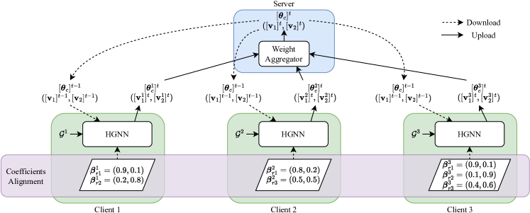
Figure 2: The overall architecture of FedHGN, with the number of clients $K=3$ and the number of bases $B=2$. Client 1 has edge types $r1$ and $r2$; client 2 has edge types $r1$ and $r3$; client 3 has edge types $r1$, $r2$, and $r3$. The uploads and downloads of $\boldsymbol{\beta}$ are not shown for brevity.

In this section, we propose FedHGN, a novel FGL framework for heterogeneous graphs and HGNNs. FedHGN aims to achieve improved HGNN performance on each client through collaborative training under a federated framework without sharing graph data, node/edge attributes, and graph schema. To attain this goal, FedHGN needs to separate graph schema from model weights before collecting and aggregating weights on the server side. Therefore, we first propose a schema-weight decoupling (SWD) strategy to enable schema-agnostic knowledge sharing in Section 4.1. Then, to alleviate the adverse side effects introduced by the decoupling strategy, we design a coefficients alignment (CA) component in Section 4.2. Next, the overall FedHGN framework is depicted in Section 4.3. Finally, a privacy analysis of our proposed framework is conducted in Section 4.4. A graphical illustration of FedHGN is provided in Figure 2.

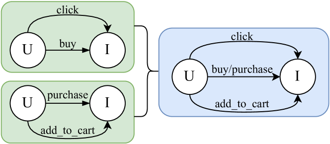
Figure 3: An example of generating the global graph schema (blue) by matching local ones (green) from two clients. FedHGN does not require this privacy-sensitive operation.

4.1 Schema-Weight Decoupling

If naively combining HGNN and conventional FL methods (e.g., FedAvg), the server and the clients would need to first coordinate for a global graph schema. Taking Figure 3 as an example, the resulting global graph schema is generated by matching the two clients’ local schemas, which inevitably breaches schema privacy and involves human expertise.

To avoid the privacy-sensitive schema matching process, we propose SWD to remove the correspondence between graph schemas and HGNN weights. For schema-specific weights $\boldsymbol{\theta}_{s}^{k}\in\mathbb{R}^{d}$ of any node/edge type $s\in\mathcal{A}\cup\mathcal{R}$ from an HGNN at client $k$, one can apply basis decomposition by

$$\boldsymbol{\theta}_{s}^{k}=\sum_{i=1}^{B}\beta_{s,i}^{k}\mathbf{v}_{i}^{k},$$ (2)

where $\beta_{s,i}^{k}\in\mathbb{R}$ are schema-specific coefficients, $\mathbf{v}_{i}^{k}\in\mathbb{R}^{d}$ are basis weights (or bases), and $B$ is a hyperparameter specifying the number of bases. Here model weights are treated as flattened vectors for notational brevity. Without loss of generality, SWD can be easily extended to higher-dimensional weights. The bases $\mathbf{v}_{i}^{k}$ are shared by all node/edge types, and not bound to the graph schema. They can be trained along with schema-irrelevant weights $\boldsymbol{\theta}_{c}^{k}$ under the conventional FL paradigm. On the other hand, a small number of coefficients $\boldsymbol{\beta}_{s}^{k}\in\mathbb{R}^{B}$ are schema-dependent. They are tuned locally at each client and do not participate in weight aggregation at the server. By applying SWD and sharing only bases, FedHGN achieves schema-agnostic knowledge sharing, which avoids graph schema leakage and manual schema matching.

4.2 Coefficients Alignment

Due to the randomness throughout training, the non-convex nature of the objective, and the non-IID heterogeneous graph data among clients, schema-specific coefficients $\boldsymbol{\beta}_{s}^{k}$ corresponding to the same node/edge type at different clients might diverge from each other towards distinct directions in the FL training process. This discrepancy between schema coefficients among clients may lead to unstable training, prolonged convergence, and sub-optimal results. Suppose the central server knows the matchings between schema coefficients among clients, this discrepancy issue can be easily resolved by aggregating and synchronizing them between the server and the clients. However, this strong assumption violates schema privacy and requires schema matching, which is not allowed in federated heterogeneous graph learning.

To address the discrepancy issue without compromising the setting, we devise a heuristic approach to align the schema coefficients by enforcing a client-side loss constraint onto them. Intuitively, even though schema coefficients of the same node/edge type at different clients may diverge in different directions, there is a high chance of them being closer in the vector space than those of the different or dissimilar node/edge types. During each communication round, in addition to the shareable bases $\mathbf{v}_{i}^{k}$ and schema-irrelevant weights $\boldsymbol{\theta}_{c}^{k}$, the FedHGN server also collects and distributes the schema-specific coefficients $\boldsymbol{\beta}_{s}^{k}$ from/to clients. But instead of aggregating them on the server side, FedHGN introduces a novel regularization term on the client side to penalize the local node/edge types’ coefficients deviating from the most similar counterpart from other clients:

$$\begin{split}\mathcal{L}_{align}^{k}=&\sum_{a\in\mathcal{A}^{k}}\min_{k^{\prime}\neq k,a^{\prime}}\left\lVert\boldsymbol{\beta}_{a}^{k}-\boldsymbol{\beta}_{a^{\prime}}^{k^{\prime}}\right\rVert_{2}^{2}+\\ &\sum_{r\in\mathcal{R}^{k}}\min_{k^{\prime}\neq k,r^{\prime}}\left\lVert\boldsymbol{\beta}_{r}^{k}-\boldsymbol{\beta}_{r^{\prime}}^{k^{\prime}}\right\rVert_{2}^{2},\end{split}$$ (3)

where $\boldsymbol{\beta}_{s}^{k}\in\mathbb{R}^{B}$ is the schema-specific coefficients of node/edge type $s\in\mathcal{A}^{k}\cup\mathcal{R}^{k}$ from client $k$’s HGNN model. The key here is how to identify the most similar counterpart for $\boldsymbol{\beta}_{s}^{k}$. We intuitively select the one with the smallest distance by taking the minimum, which has the highest chance of matching the node/edge type. By minimizing this heuristic regularization term, FedHGN aligns schema coefficients across clients without disclosing actual graph schema.

Algorithm 1 FedHGN framework.

1:$K$ clients indexed by $k$; Client sampling fraction $C$; Number of bases $B$; Number of local epochs $E$; Learning rate $\eta$; Alignment regularization factor $\lambda$.

2:procedure ServerExecution

3:   Initialize $[\boldsymbol{\theta}_{c}]^{0}$, $[\mathbf{v}]^{0}$, and $\{[\boldsymbol{\beta}^{k}]^{0}:1\leq k\leq K\}$ (subscripts of $\mathbf{v}$ and $\boldsymbol{\beta}$ omitted for brevity)

4:   for round $t=1,2,\ldots$ do

5:      $\mathcal{S}_{t}\leftarrow$ (random set of $\max(C\cdot K,1)$ clients)

6:      for each client $k\in\mathcal{S}_{t}$ in parallel do

7:         $[\boldsymbol{\theta}_{c}^{k}]^{t},[\mathbf{v}^{k}]^{t},[\boldsymbol{\beta}^{k}]^{t}\leftarrow\operatorname{ClientUpdate}($

8:           $k,[\boldsymbol{\theta}_{c}]^{t-1},[\mathbf{v}]^{t-1},\{[\boldsymbol{\beta}^{k^{\prime}}]^{t-1}:k^{\prime}\neq k\})$

9:      end for

10:      $([\boldsymbol{\theta}_{c}]^{t},[\mathbf{v}]^{t})\leftarrow\sum_{k\in\mathcal{S}_{t}}\frac{N_{k}}{N_{\mathcal{S}_{t}}}([\boldsymbol{\theta}_{c}^{k}]^{t},[\mathbf{v}^{k}]^{t})$

11:      $[\boldsymbol{\beta}^{k}]^{t}\leftarrow[\boldsymbol{\beta}^{k}]^{t-1},\forall k\notin\mathcal{S}_{t}$

12:   end for

13:end procedure

14:procedure ClientUpdate($k$, $\boldsymbol{\theta}_{c}$, $\mathbf{v}$, $\{\boldsymbol{\beta}^{k^{\prime}}:k^{\prime}\neq k\}$)

15:   $\boldsymbol{\theta}_{s}\leftarrow\sum_{i=1}^{B}\beta_{s,i}^{k}\mathbf{v}_{i},\forall s\in\mathcal{A}^{k}\cup\mathcal{R}^{k}$

16:   for epoch $i=1,2,\ldots,E$ do

17:      for minibatch $m$ sampled from $\mathcal{D}^{k}$ do

18:         $\mathcal{L}_{task}^{k}\leftarrow$ (task-specific loss given $m$)

19:         $\mathcal{L}_{align}^{k}\leftarrow$ Equation (3)

20:         $\boldsymbol{\theta}_{c},\mathbf{v},\boldsymbol{\beta}^{k}\leftarrow(\boldsymbol{\theta}_{c},\mathbf{v},\boldsymbol{\beta}^{k})-\eta\nabla\left(\mathcal{L}_{task}^{k}+\lambda\mathcal{L}_{align}^{k}\right)$

21:      end for

22:   end for

23:   Return $\boldsymbol{\theta}_{c}$, $\mathbf{v}$, and $\boldsymbol{\beta}^{k}$ to server

24:end procedure

4.3 Framework Overview

Our FedHGN framework largely follows FedAvg, which iteratively conducts local training at multiple clients and weight aggregation at a central server. In addition to the typical operations of FedAvg, FedHGN employs SWD and CA to preserve schema privacy without performance degradation. Before starting the federated training process, the server and the clients would negotiate for the hyperparameters of the HGNN model used, such as the number of bases ($B$) in SWD. The primary training process comprises many communication rounds between the server and the clients. The detailed server-side and client-side operations of a single round in FedHGN are described below. Figure 2 illustrates this training process. Complete pseudocode is given in Algorithm 1.

Server Operations.

At round $t$, the server first samples a fraction of clients $\mathcal{S}_{t}$ for this round of training. The server then sends the latest model parameters to each client $k\in\mathcal{S}_{t}$, including the aggregated schema-agnostic weights, $[\boldsymbol{\theta}_{c}]^{t-1}$ and $[\mathbf{v}_{i}]^{t-1}$, and collected schema coefficients $[\boldsymbol{\beta}_{s}^{k^{\prime}}]^{t-1}$ from the previous round. After client-side local updates, the server receives the updated $[\boldsymbol{\theta}_{c}^{k}]^{t}$, $[\mathbf{v}_{i}^{k}]^{t}$, and $[\boldsymbol{\beta}_{s}^{k}]^{t}$ from each $k\in\mathcal{S}_{t}$. Finally, the server aggregates the schema-agnostic weights by $[\boldsymbol{\theta}_{c}]^{t}=\sum_{k\in\mathcal{S}_{t}}\frac{N_{k}}{N_{\mathcal{S}_{t}}}[\boldsymbol{\theta}_{c}^{k}]^{t}$ and $[\mathbf{v}_{i}]^{t}=\sum_{k\in\mathcal{S}_{t}}\frac{N_{k}}{N_{\mathcal{S}_{t}}}[\mathbf{v}_{i}^{k}]^{t}$, where $N_{k}$ is the number of training samples at client $k$, and $N_{\mathcal{S}_{t}}=\sum_{k\in\mathcal{S}_{t}}N_{k}$ is the total number of training samples of this round. The server also sets $[\boldsymbol{\beta}_{s}^{k}]^{t}=[\boldsymbol{\beta}_{s}^{k}]^{t-1}$ for $k\notin\mathcal{S}_{t}$.

Client Operations.

At round $t$, each selected client $k$ receives the latest model parameters from the server, including schema-agnostic weights, $[\boldsymbol{\theta}_{c}]^{t-1}$ and $[\mathbf{v}_{i}]^{t-1}$, and other clients’ schema coefficients $[\boldsymbol{\beta}_{s}^{k^{\prime}}]^{t-1}$. The schema-specific weights are recreated via Equation (2). Then, the client would conduct local training using local heterogeneous graph data $\mathcal{D}^{k}$ for several epochs to tune model parameters. The client-side objective function is a sum of the task-specific loss and the CA regularization term: $\mathcal{L}^{k}=\mathcal{L}_{task}^{k}+\lambda\mathcal{L}_{align}^{k}$, where $\mathcal{L}_{task}^{k}$ could be cross entropy for node classification tasks or some ranking loss for link prediction tasks. Finally, the client uploads the updated schema-agnostic HGNN weights, $[\boldsymbol{\theta}_{c}^{k}]^{t}$ and $[\mathbf{v}_{i}^{k}]^{t}$, and schema coefficients $[\boldsymbol{\beta}_{s}^{k}]^{t}$ back to the server.

4.4 Privacy Analysis

In this section, we analyze the communications between the server and the clients and discuss whether FedHGN can preserve the data privacy of local graph schemas.

Server-side Analysis.

FedHGN server is restricted to collecting limited information that cannot be used to infer graph schemas of any clients. The central server receives only HGNN model weights $\mathbf{v}_{i}^{k}$, $\boldsymbol{\theta}_{c}^{k}$, and $\boldsymbol{\beta}_{s}^{k}$ from each client. $\mathbf{v}_{i}^{k}$ and $\boldsymbol{\theta}_{c}^{k}$ are schema-agnostic model weights, revealing no schema information. Although $\boldsymbol{\beta}_{s}^{k}$ are schema-specific coefficients, the server can only deduce the number of node/edge types in each client. It still cannot learn other meaningful schema information, like the matching among them or the physical name of their corresponding node/edge types.

Client-side Analysis.

Data privacy at each client is well protected under the FedHGN framework. Each client $k$ receives $\mathbf{v}_{i}$, $\boldsymbol{\theta}_{c}$, and $\boldsymbol{\beta}_{s}^{k^{\prime}}$ (for $k^{\prime}\neq k$) from the server. Similarly, clients cannot infer other clients’ graph schemas from $\mathbf{v}_{i}$ and $\boldsymbol{\theta}_{c}$. Since the schema-specific coefficients $\boldsymbol{\beta}_{s}^{k^{\prime}}$ are sent to client $k$ as an unordered set, client $k$ cannot differentiate the source client of each received $\boldsymbol{\beta}_{s}^{k^{\prime}}$. Therefore, neither the HGNN model nor the graph schema of any other client can be derived based on what client $k$ receives from the server.

$K$		3	5	10
RE	# ntypes	27.0	27.0	27.0
	# etypes	120.7	122.0	120.0
	# nodes	80,592.0	68,697.6	50,238.5
	# edges	358,873.3	249,948.4	142,849.6
RET	# ntypes	20.3	18.0	12.3
	# etypes	66.0	52.4	26.8
	# nodes	77,027.7	73,202.4	43,735.6
	# edges	349,813.3	248,125.6	138,807.0

Table 2: Averaged statistics of the BGS dataset split into $K$ clients.

Dataset		AIFB			MUTAG		BGS
Central		87.78$\pm$2.22			68.24$\pm$3.79		81.38$\pm$1.69
$K$		3	5	10	5	10	5	10
RE	Local	74.77$\pm$5.22	71.30$\pm$4.30	55.08$\pm$1.09	65.06$\pm$1.28	64.88$\pm$1.12	67.04$\pm$1.79	64.54$\pm$1.65
	FedAvg	74.02$\pm$3.09	65.18$\pm$3.59	54.95$\pm$1.42	65.06$\pm$0.34	65.47$\pm$0.74	67.36$\pm$2.52	65.04$\pm$1.26
	FedProx	72.34$\pm$3.37	65.29$\pm$5.43	53.38$\pm$2.79	65.59$\pm$0.69	65.62$\pm$0.76	66.11$\pm$3.99	63.97$\pm$1.66
	FedHGN	81.87$\pm$2.33	72.94$\pm$3.27	59.32$\pm$1.42	67.87$\pm$0.83	65.59$\pm$0.86	67.52$\pm$2.58	65.73$\pm$1.47
RET	Local	76.11$\pm$3.58	65.89$\pm$2.29	59.71$\pm$3.06	64.78$\pm$0.89	64.18$\pm$3.13	67.73$\pm$1.19	67.11$\pm$0.52
	FedAvg	80.00$\pm$1.72	66.56$\pm$3.47	59.59$\pm$3.03	66.04$\pm$0.11	66.28$\pm$0.15	69.10$\pm$2.11	65.04$\pm$0.96
	FedProx	80.93$\pm$2.78	66.00$\pm$2.95	60.99$\pm$1.95	65.92$\pm$0.29	66.13$\pm$0.06	70.62$\pm$1.42	66.07$\pm$0.80
	FedHGN	86.55$\pm$2.53	70.67$\pm$2.42	66.76$\pm$3.22	66.21$\pm$0.40	66.21$\pm$0.12	69.79$\pm$2.07	69.03$\pm$1.44

Table 3: Experimental results (weighted average of accuracy %) of node classification.

5 Experiments

In this section, we demonstrate the effectiveness of FedHGN on federated learning of HGNNs by conducting experiments for node classification on a series of heterogeneous graph datasets. The experiments are designed to answer the following research questions. RQ1: Can FedHGN achieve a better HGNN performance than purely local training? RQ2: Can FedHGN outperform conventional FL methods in training HGNNs? RQ3: What are the effects of the proposed schema-weight decoupling and coefficients alignment? RQ4: How is FedHGN affected by the hyperparameters?

5.1 Experimental Setup

Datasets.

We select widely-adopted heterogeneous graph datasets for our node classification experiments: AIFB, MUTAG, and BGS preprocessed by Deep Graph Library (DGL) Wang et al. (2019a). These datasets are highly heterogeneous with more than 50 node/edge types. To simulate the federated setting, we randomly split each dataset into $K=3$, $5$, and $10$ clients. We propose two random splitting strategies for heterogeneous graphs: (1) Random Edges (RE) which randomly allocates edges to $K$ clients and (2) Random Edge Types (RET) which randomly allocates edge types to $K$ clients. RE simulates a scenario where each client owns a part of the complete graph, within which there are overlapping nodes/edges among clients. RET simulates a more complex scenario where clients construct the local heterogeneous graphs differently, resulting in distinct graph schemas. Averaged statistics of the BGS dataset split into $K$ clients are summarized in Table 2. More details about the datasets and splitting strategies are provided in the appendix.

Baselines.

To assess FedHGN and demonstrate its superiority, we choose the following settings/algorithms as baselines: (1) centralized training, (2) local training, (3) FedAvg, and (4) FedProx. We do not include existing FGL methods as baselines because they cannot be easily adapted to HGNNs. FedAlign is not adopted because its source code is not available and some design details are not disclosed in its paper.

Implementation.

We employ an RGCN-like architecture as the HGNN model. Other details are in the appendix.

5.2 Experimental Results

We report results averaged from 5 runs using different random seeds. The accuracy score of each run is computed via a weighted average of the $K$ clients’ local testing scores based on the numbers of their testing samples.

5.2.1 Main Results (RQ1 & RQ2)

To evaluate FedHGN against local training and conventional FL algorithms, we conduct comprehensive experiments on three datasets with varying client numbers. Note that schema sharing is required and allowed in FedAvg and FedProx, but not in FedHGN. Averaged accuracy scores with standard deviations are listed in Table 3. Due to the space limit, we leave the $K=3$ settings of MUTAG and BGS in the appendix.

As shown in the table, FedHGN consistently outperforms local training and conventional FL algorithms in most settings. As expected, HGNN performance deteriorates in local training due to insufficient data, especially on AIFB and BGS. But conventional FL algorithms (FedAvg and FedProx) do not have a noticeable advantage over local training in our experiments. On AIFB (RE), they are even outperformed by the local setting. Although FedProx is designed to alleviate the non-IID data issue, it cannot correctly handle heterogeneous graph data based on our results. Compared to FedAvg and FedProx, FedHGN makes no compromise in schema-level privacy and yet achieves superior results, showing that FedHGN is a better option for federated HGNNs. FedHGN’s advantage in preserving HGNN performance might come from the decoupled schema coefficients. They may serve as personalized model parameters to help each client combat the severe non-IID problem of heterogeneous graphs.

SWD	CA	MUTAG (RE)		BGS (RE)
		$K=5$	$K=10$	$K=5$	$K=10$
B	✗	63.18	60.59	66.39	59.36
C	✗	65.88	61.26	67.78	64.11
B+C	✗	65.29	62.83	66.53	63.76
✗	✗	65.06	65.47	67.36	65.04
B	✓	67.87	65.59	67.52	65.73

Table 4: Ablation study on the MUTAG and BGS datasets (RE splitting strategy). B: aggregating basis weights. C: aggregating schema-specific coefficients. The last row is our proposed FedHGN.

5.2.2 Ablation Study (RQ3)

To analyze the effects of the proposed designs, we compare variants of FedHGN on MUTAG (RE) and BGS (RE) in Table 4 by applying different schema-weight decoupling (SWD) strategies and whether employing coefficients alignment (CA) or not. The table shows that CA brings about a 7% improvement compared to the variant without it. We also notice a longer convergence time when removing CA. Therefore, the alignment component is necessary for FedHGN to stabilize training and maintain performance. For SWD, we observe that additionally aggregating schema coefficients at the server side (breaking schema privacy) leads to some performance gain, which can be well compensated by CA. Another interesting observation is that the FedHGN variant that only aggregates schema coefficients achieves decent results. We suspect it may resemble the local setting because the shared coefficients have a small parameter space. We also present the results produced by removing both SWD and CA, which reduces FedHGN to FedAvg. Although outperforming the variant that uses only SWD, FedAvg violates schema privacy and is still inferior to the full version of FedHGN. All these results confirm the effectiveness of SWD and CA.

5.2.3 Hyperparameter Analysis (RQ4)

To investigate how FedHGN is affected by the newly introduced hyperparameters, we conduct pilot tests on AIFB with different choices for the number of bases $B$ and the alignment regularization factor $\lambda$. Except for the concerning hyperparameter, all other setups are kept unchanged. From Figure 4, we find that FedHGN is sensitive to the choice of $B$. The optimal performance is reached at around $B=35$ and $B=20$ for AIFB (RE) and AIFB (RET), respectively. Intuitively, $B$ should be related to the number of edge types involved in the FL system. Since other settings (MUTAG and BGS) contain a similar or smaller number of edge types, we roughly choose $B=20$ as a sugar point to report the main results.

For the alignment regularization factor $\lambda$, FedHGN performance does not change much when $\lambda$ is reasonable, i.e., for $\lambda\leq 5$. But when $\lambda$ gets larger than 5, the testing accuracy drops dramatically on both AIFB (RE) and AIFB (RET). When $\lambda$ is too large, the optimization objective is dominated by the CA regularization term $\mathcal{L}_{align}$. HGNNs cannot learn much knowledge from the task-specific loss $\mathcal{L}_{task}$ in this case. Hence, we just set $\lambda=0.5$ for our main experiments.

6 Discussion

This work aims to avoid schema matching and ensure schema privacy during federated HGNN learning. By carefully examining the HGNN architecture, we notice the crux of the matter is the correspondence between model weights and node/edge types. Our FedHGN is designed to decouple this binding and achieve schema-agnostic weight sharing. This seems unnecessary as one could just apply secure multiparty computation (MPC) techniques like private set operations Freedman et al. (2004); Kissner and Song (2005) to match the node/edge types across clients. However, node/edge types’ naming conventions may differ across clients. Human labor is usually inevitable to coordinate a set of naming rules, which generally breaks schema privacy. Furthermore, without SWD, the server can derive client schema from received gradient/weight changes between communication rounds. Although gradients can be protected by differential privacy Abadi et al. (2016), homomorphic encryption Phong et al. (2018), secure aggregation Bonawitz et al. (2017), or MPC Mohassel and Zhang (2017), these approaches could affect model performance, increase computational overhead, or impede communication reduction methods Ergün et al. (2022). Therefore, we reckon FedHGN as a practical design to reduce schema privacy risks.

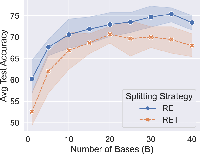
(a) The number of bases ($B$).

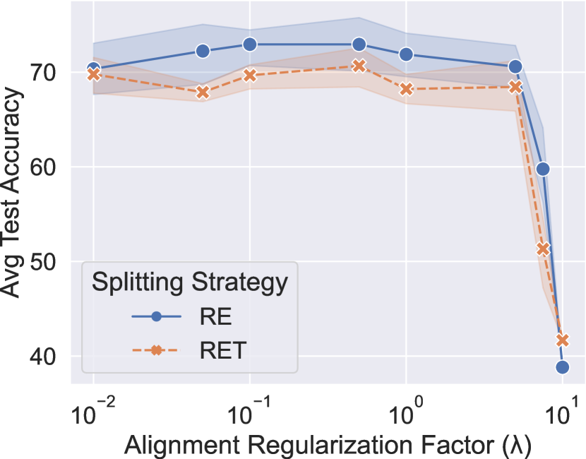
(b) The alignment factor ($\lambda$).

Figure 4: Hyperparameter analysis of varying $B$ and $\lambda$.

7 Conclusion

This paper proposes FedHGN, a novel federated heterogeneous graph learning framework for HGNNs with schema privacy protection. By decoupling graph schemas and model weights, FedHGN removes the correspondence between node/edge types and HGNN weights to achieve schema-agnostic knowledge sharing. With an alignment regularization term, the discrepancy among same-type schema coefficients across clients is alleviated to stabilize training and boost model performance. Experimental results show that FedHGN can bring consistent performance improvement to HGNNs while preserving both data and schema privacy, outperforming local training and conventional FL algorithms.

Appendix A Datasets

We select widely-adopted heterogeneous graph datasets for our node classification experiments. Specifically, we adopt three datasets in Resource Description Framework (RDF) format: AIFB, MUTAG, and BGS preprocessed by Deep Graph Library (DGL) Wang et al. [2019a].

To simulate a federated training setting, we propose two random splitting strategies as follows. Averaged statistics of the datasets split into $K$ clients are summarized in Table 5.

• Random edges (RE). The edges of the given graph are randomly and evenly divided into $K+2$ groups. Each client exclusively possesses one group of edges. All clients share another group of edges. The edges in the remaining group are distributed to randomly selected $p$ ($1<p<K$) clients.

• Random edge types (RET). The edge types of the given graph are randomly and evenly divided into $K+2$ groups. Each client exclusively possesses one group of edge types. All clients share another group of edge types. The edge types in the remaining group are distributed to randomly selected $p$ ($1<p<K$) clients.

Dataset		AIFB			MUTAG			BGS
$K$		3	5	10	3	5	10	3	5	10
RE	# ntypes	7.0	7.0	7.0	5.0	5.0	5.0	27.0	27.0	27.0
	# etypes	104.0	103.2	101.6	50.0	50.0	49.0	120.7	122.0	120.0
	# nodes	4,818.7	3,916.8	2,941.3	22,969.0	19,961.2	14,661.6	80,592.0	68,697.6	50,238.5
	# edges	26,032.0	18,140.8	10,390.6	78,986.7	54,976.8	31,489.8	358,873.3	249,948.4	142,849.6
	# train	110.7	105.8	94.1	218.0	217.8	217.1	94.0	93.8	92.6
	# valid	27.7	27.8	25.2	54.0	54.0	54.0	23.0	23.0	22.6
	# test	35.7	34.0	29.3	68.0	68.0	68.0	29.0	28.8	28.2
RET	# ntypes	7.0	6.4	6.0	4.3	4.2	3.7	20.3	18.0	12.3
	# etypes	57.3	43.2	28.8	26.7	23.6	13.0	66.0	52.4	26.8
	# nodes	4,600.0	3,936.2	2,632.0	20,185.7	24,098.4	19,670.1	77,027.7	73,202.4	43,735.6
	# edges	26,110.0	22,079.2	17,115.6	77,898.7	76,971.2	49,366.6	349,813.3	248,125.6	138,807.0
	# train	112.0	112.0	107.9	218.0	212.4	207.1	94.0	94.0	94.0
	# valid	28.0	28.0	26.9	54.0	53.0	52.4	23.0	23.0	23.0
	# test	36.0	36.0	34.2	68.0	67.0	66.2	29.0	29.0	29.0

Table 5: Averaged statistics of the datasets after being split into $K$ clients.

Appendix B Baselines

To assess FedHGN and fully demonstrate its superiority, we choose the following three types of settings/algorithms as baselines: (1) centralized training, (2) local training, and (3) two conventional FL algorithms: FedAvg McMahan et al. [2017] and FedProx Li et al. [2020].

• Central. The HGNN is trained using the complete graph without data splitting.

• Local. The HGNN is trained separately for each client using only local heterogeneous graph data.

• FedAvg. The HGNN is trained using FedAvg without schema-weight decoupling and coefficients alignment. This FL setting assumes graph schemas are shared and matched, breaching schema privacy.

• FedProx. This one is similar to the FedAvg setting above. The loss function contains a proximal term to reduce the influence of system and data heterogeneity. This FL setting assumes graph schemas are shared and matched, breaching schema privacy.

Appendix C Implementation Details

We employ an RGCN-like architecture as the HGNN model, which ignores node types and decouples edge-type-specific weights. Throughout the experiments, unless otherwise specified, we fix the client sampling fraction $C=1.0$, the embedding dimension $d=64$, the number of HGNN layers $L=2$, the number of bases $B=20$, the alignment regularization factor $\lambda=0.5$, the number of local epochs $E=3$, and the early stopping patience as 10 rounds. We perform full-batch training using a stochastic gradient descent (SGD) optimizer with a learning rate $\eta=0.1$. For baselines, we keep applicable hyperparameters to be the same as above for a fair comparison. We implement FedHGN and all baselines using the PyTorch and DGL packages, and conduct all experiments on one NVIDIA RTX 3090 GPU.

Appendix D More Experimental Results

Due to the space limit of the main body, we provide the complete experimental results here. Results on the AIFB dataset are provided in Table 6. Results on the MUTAG dataset are provided in Table 7. Results on the BGS dataset are provided in Table 8. Ablation study results with standard deviations are provided in Table 9.

Dataset		AIFB
Central		87.78$\pm$2.22
$K$		3	5	10
RE	Local	74.77$\pm$5.22	71.30$\pm$4.30	55.08$\pm$1.09
	FedAvg	74.02$\pm$3.09	65.18$\pm$3.59	54.95$\pm$1.42
	FedProx	72.34$\pm$3.37	65.29$\pm$5.43	53.38$\pm$2.79
	FedHGN	81.87$\pm$2.33	72.94$\pm$3.27	59.32$\pm$1.42
RET	Local	76.11$\pm$3.58	65.89$\pm$2.29	59.71$\pm$3.06
	FedAvg	80.00$\pm$1.72	66.56$\pm$3.47	59.59$\pm$3.03
	FedProx	80.93$\pm$2.78	66.00$\pm$2.95	60.99$\pm$1.95
	FedHGN	86.55$\pm$2.53	70.67$\pm$2.42	66.76$\pm$3.22

Table 6: Experimental results (weighted average of accuracy %) of node classification on the AIFB dataset.

Dataset		MUTAG
Central		68.24$\pm$3.79
$K$		3	5	10
RE	Local	63.53$\pm$1.77	65.06$\pm$1.28	64.88$\pm$1.12
	FedAvg	64.42$\pm$1.18	65.06$\pm$0.34	65.47$\pm$0.74
	FedProx	66.08$\pm$3.46	65.59$\pm$0.69	65.62$\pm$0.76
	FedHGN	67.06$\pm$1.26	67.87$\pm$0.83	65.59$\pm$0.86
RET	Local	63.24$\pm$0.62	64.78$\pm$0.89	64.18$\pm$3.13
	FedAvg	64.61$\pm$1.33	66.04$\pm$0.11	66.28$\pm$0.15
	FedProx	65.30$\pm$2.45	65.92$\pm$0.29	66.13$\pm$0.06
	FedHGN	65.98$\pm$2.86	66.21$\pm$0.40	66.21$\pm$0.12

Table 7: Experimental results (weighted average of accuracy %) of node classification on the MUTAG dataset.

Dataset		BGS
Central		81.38$\pm$1.69
$K$		3	5	10
RE	Local	67.36$\pm$3.66	67.04$\pm$1.79	64.54$\pm$1.65
	FedAvg	68.28$\pm$3.95	67.36$\pm$2.52	65.04$\pm$1.26
	FedProx	68.28$\pm$2.96	66.11$\pm$3.99	63.97$\pm$1.66
	FedHGN	69.20$\pm$3.22	67.52$\pm$2.58	65.73$\pm$1.47
RET	Local	75.63$\pm$4.07	67.73$\pm$1.19	67.11$\pm$0.52
	FedAvg	76.09$\pm$1.34	69.10$\pm$2.11	65.04$\pm$0.96
	FedProx	76.32$\pm$2.13	70.62$\pm$1.42	66.07$\pm$0.80
	FedHGN	78.93$\pm$2.23	69.79$\pm$2.07	69.03$\pm$1.44

Table 8: Experimental results (weighted average of accuracy %) of node classification on the BGS dataset.

SWD	CA	MUTAG (RE)		BGS (RE)
		$K=5$	$K=10$	$K=5$	$K=10$
B	✗	63.18$\pm$2.73	60.59$\pm$1.28	66.39$\pm$3.12	59.36$\pm$2.54
C	✗	65.88$\pm$0.46	61.26$\pm$1.33	67.78$\pm$2.09	64.11$\pm$2.40
B+C	✗	65.29$\pm$0.93	62.83$\pm$3.13	66.53$\pm$2.93	63.76$\pm$0.61
✗	✗	65.06$\pm$0.34	65.47$\pm$0.74	67.36$\pm$2.52	65.04$\pm$1.26
B	✓	67.87$\pm$0.83	65.59$\pm$0.86	67.52$\pm$2.58	65.73$\pm$1.47

Table 9: Ablation study on the MUTAG and BGS datasets (RE splitting strategy). B: aggregating basis weights. C: aggregating schema-specific coefficients. The last row is our proposed FedHGN.

References

- Abadi et al. [2016] Martín Abadi, Andy Chu, Ian J. Goodfellow, H. Brendan McMahan, Ilya Mironov, Kunal Talwar, and Li Zhang. Deep learning with differential privacy. In CCS, pages 308–318. ACM, 2016.
- Bonawitz et al. [2017] Kallista A. Bonawitz, Vladimir Ivanov, Ben Kreuter, Antonio Marcedone, H. Brendan McMahan, Sarvar Patel, Daniel Ramage, Aaron Segal, and Karn Seth. Practical secure aggregation for privacy-preserving machine learning. In CCS, pages 1175–1191. ACM, 2017.
- Chen et al. [2019] Zhengdao Chen, Lisha Li, and Joan Bruna. Supervised community detection with line graph neural networks. In ICLR (Poster). OpenReview.net, 2019.
- Chen et al. [2021] Mingyang Chen, Wen Zhang, Zonggang Yuan, Yantao Jia, and Huajun Chen. Fede: Embedding knowledge graphs in federated setting. In IJCKG, pages 80–88. ACM, 2021.
- Chen et al. [2022] Yankai Chen, Menglin Yang, Yingxue Zhang, Mengchen Zhao, Ziqiao Meng, Jianye Hao, and Irwin King. Modeling scale-free graphs with hyperbolic geometry for knowledge-aware recommendation. In WSDM, pages 94–102. ACM, 2022.
- Defferrard et al. [2016] Michaël Defferrard, Xavier Bresson, and Pierre Vandergheynst. Convolutional neural networks on graphs with fast localized spectral filtering. In NIPS, pages 3837–3845, 2016.
- Ergün et al. [2022] Irem Ergün, Hasin Us Sami, and Basak Güler. Communication-efficient secure aggregation for federated learning. In GLOBECOM, pages 3881–3886. IEEE, 2022.
- Freedman et al. [2004] Michael J. Freedman, Kobbi Nissim, and Benny Pinkas. Efficient private matching and set intersection. In EUROCRYPT, volume 3027 of Lecture Notes in Computer Science, pages 1–19. Springer, 2004.
- Fu et al. [2020] Xinyu Fu, Jiani Zhang, Ziqiao Meng, and Irwin King. MAGNN: metapath aggregated graph neural network for heterogeneous graph embedding. In WWW, pages 2331–2341. ACM / IW3C2, 2020.
- Grover and Leskovec [2016] Aditya Grover and Jure Leskovec. node2vec: Scalable feature learning for networks. In KDD, pages 855–864. ACM, 2016.
- Hamilton et al. [2017] William L. Hamilton, Zhitao Ying, and Jure Leskovec. Inductive representation learning on large graphs. In NIPS, pages 1024–1034, 2017.
- Hu et al. [2020] Ziniu Hu, Yuxiao Dong, Kuansan Wang, and Yizhou Sun. Heterogeneous graph transformer. In WWW, pages 2704–2710. ACM / IW3C2, 2020.
- Jin et al. [2019] Di Jin, Ziyang Liu, Weihao Li, Dongxiao He, and Weixiong Zhang. Graph convolutional networks meet markov random fields: Semi-supervised community detection in attribute networks. In AAAI, pages 152–159. AAAI Press, 2019.
- Karimireddy et al. [2020] Sai Praneeth Karimireddy, Satyen Kale, Mehryar Mohri, Sashank J. Reddi, Sebastian U. Stich, and Ananda Theertha Suresh. SCAFFOLD: stochastic controlled averaging for federated learning. In ICML, volume 119 of Proceedings of Machine Learning Research, pages 5132–5143. PMLR, 2020.
- Kipf and Welling [2017] Thomas N. Kipf and Max Welling. Semi-supervised classification with graph convolutional networks. In ICLR (Poster). OpenReview.net, 2017.
- Kissner and Song [2005] Lea Kissner and Dawn Xiaodong Song. Privacy-preserving set operations. In CRYPTO, volume 3621 of Lecture Notes in Computer Science, pages 241–257. Springer, 2005.
- Li et al. [2018] Yaguang Li, Rose Yu, Cyrus Shahabi, and Yan Liu. Diffusion convolutional recurrent neural network: Data-driven traffic forecasting. In ICLR (Poster). OpenReview.net, 2018.
- Li et al. [2020] Tian Li, Anit Kumar Sahu, Manzil Zaheer, Maziar Sanjabi, Ameet Talwalkar, and Virginia Smith. Federated optimization in heterogeneous networks. In MLSys. mlsys.org, 2020.
- Li et al. [2022] Jingjing Li, Zichao Li, Tao Ge, Irwin King, and Michael R. Lyu. Text revision by on-the-fly representation optimization. In AAAI, pages 10956–10964. AAAI Press, 2022.
- Lin et al. [2020] Yilun Lin, Chaochao Chen, Cen Chen, and Li Wang. Improving federated relational data modeling via basis alignment and weight penalty. CoRR, abs/2011.11369, 2020.
- Lv et al. [2021] Qingsong Lv, Ming Ding, Qiang Liu, Yuxiang Chen, Wenzheng Feng, Siming He, Chang Zhou, Jianguo Jiang, Yuxiao Dong, and Jie Tang. Are we really making much progress?: Revisiting, benchmarking and refining heterogeneous graph neural networks. In KDD, pages 1150–1160. ACM, 2021.
- Ma et al. [2022] Yueen Ma, Zixing Song, Xuming Hu, Jingjing Li, Yifei Zhang, and Irwin King. Graph component contrastive learning for concept relatedness estimation, 2022.
- McMahan et al. [2017] Brendan McMahan, Eider Moore, Daniel Ramage, Seth Hampson, and Blaise Agüera y Arcas. Communication-efficient learning of deep networks from decentralized data. In AISTATS, volume 54 of Proceedings of Machine Learning Research, pages 1273–1282. PMLR, 2017.
- Mohassel and Zhang [2017] Payman Mohassel and Yupeng Zhang. Secureml: A system for scalable privacy-preserving machine learning. In IEEE Symposium on Security and Privacy, pages 19–38. IEEE Computer Society, 2017.
- Peng et al. [2021] Hao Peng, Haoran Li, Yangqiu Song, Vincent W. Zheng, and Jianxin Li. Differentially private federated knowledge graphs embedding. In CIKM, pages 1416–1425. ACM, 2021.
- Perozzi et al. [2014] Bryan Perozzi, Rami Al-Rfou, and Steven Skiena. Deepwalk: online learning of social representations. In KDD, pages 701–710. ACM, 2014.
- Phong et al. [2018] Le Trieu Phong, Yoshinori Aono, Takuya Hayashi, Lihua Wang, and Shiho Moriai. Privacy-preserving deep learning via additively homomorphic encryption. IEEE Trans. Inf. Forensics Secur., 13(5):1333–1345, 2018.
- Schlichtkrull et al. [2018] Michael Sejr Schlichtkrull, Thomas N. Kipf, Peter Bloem, Rianne van den Berg, Ivan Titov, and Max Welling. Modeling relational data with graph convolutional networks. In ESWC, volume 10843 of Lecture Notes in Computer Science, pages 593–607. Springer, 2018.
- Tang et al. [2015] Jian Tang, Meng Qu, Mingzhe Wang, Ming Zhang, Jun Yan, and Qiaozhu Mei. LINE: large-scale information network embedding. In WWW, pages 1067–1077. ACM, 2015.
- van den Berg et al. [2017] Rianne van den Berg, Thomas N. Kipf, and Max Welling. Graph convolutional matrix completion. CoRR, abs/1706.02263, 2017.
- Velickovic et al. [2018] Petar Velickovic, Guillem Cucurull, Arantxa Casanova, Adriana Romero, Pietro Liò, and Yoshua Bengio. Graph attention networks. In ICLR (Poster). OpenReview.net, 2018.
- Wang et al. [2019a] Minjie Wang, Lingfan Yu, Da Zheng, Quan Gan, Yu Gai, Zihao Ye, Mufei Li, Jinjing Zhou, Qi Huang, Chao Ma, Ziyue Huang, Qipeng Guo, Hao Zhang, Haibin Lin, Junbo Zhao, Jinyang Li, Alexander J. Smola, and Zheng Zhang. Deep graph library: Towards efficient and scalable deep learning on graphs. CoRR, abs/1909.01315, 2019.
- Wang et al. [2019b] Xiao Wang, Houye Ji, Chuan Shi, Bai Wang, Yanfang Ye, Peng Cui, and Philip S. Yu. Heterogeneous graph attention network. In WWW, pages 2022–2032. ACM, 2019.
- Wu et al. [2019] Felix Wu, Amauri H. Souza Jr., Tianyi Zhang, Christopher Fifty, Tao Yu, and Kilian Q. Weinberger. Simplifying graph convolutional networks. In ICML, volume 97 of Proceedings of Machine Learning Research, pages 6861–6871. PMLR, 2019.
- Wu et al. [2021] Chuhan Wu, Fangzhao Wu, Yang Cao, Yongfeng Huang, and Xing Xie. Fedgnn: Federated graph neural network for privacy-preserving recommendation. CoRR, abs/2102.04925, 2021.
- Xie et al. [2021] Han Xie, Jing Ma, Li Xiong, and Carl Yang. Federated graph classification over non-iid graphs. In NeurIPS, pages 18839–18852, 2021.
- Xu et al. [2019] Keyulu Xu, Weihua Hu, Jure Leskovec, and Stefanie Jegelka. How powerful are graph neural networks? In ICLR. OpenReview.net, 2019.
- Yang et al. [2022] Menglin Yang, Min Zhou, Jiahong Liu, Defu Lian, and Irwin King. HRCF: enhancing collaborative filtering via hyperbolic geometric regularization. In WWW, pages 2462–2471. ACM, 2022.
- Ying et al. [2018] Rex Ying, Ruining He, Kaifeng Chen, Pong Eksombatchai, William L. Hamilton, and Jure Leskovec. Graph convolutional neural networks for web-scale recommender systems. In KDD, pages 974–983. ACM, 2018.
- Yu et al. [2018] Bing Yu, Haoteng Yin, and Zhanxing Zhu. Spatio-temporal graph convolutional networks: A deep learning framework for traffic forecasting. In IJCAI, pages 3634–3640. ijcai.org, 2018.
- Yun et al. [2019] Seongjun Yun, Minbyul Jeong, Raehyun Kim, Jaewoo Kang, and Hyunwoo J. Kim. Graph transformer networks. In NeurIPS, pages 11960–11970, 2019.
- Zhang and Zhu [2020] Yifei Zhang and Hao Zhu. Additively homomorphical encryption based deep neural network for asymmetrically collaborative machine learning. CoRR, abs/2007.06849, 2020.
- Zhang et al. [2018] Jiani Zhang, Xingjian Shi, Junyuan Xie, Hao Ma, Irwin King, and Dit-Yan Yeung. Gaan: Gated attention networks for learning on large and spatiotemporal graphs. In UAI, pages 339–349. AUAI Press, 2018.
- Zhang et al. [2019] Chuxu Zhang, Dongjin Song, Chao Huang, Ananthram Swami, and Nitesh V. Chawla. Heterogeneous graph neural network. In KDD, pages 793–803. ACM, 2019.
- Zhang et al. [2021] Ke Zhang, Carl Yang, Xiaoxiao Li, Lichao Sun, and Siu-Ming Yiu. Subgraph federated learning with missing neighbor generation. In NeurIPS, pages 6671–6682, 2021.
- Zhang et al. [2022a] Yifei Zhang, Hao Zhu, Ziqiao Meng, Piotr Koniusz, and Irwin King. Graph-adaptive rectified linear unit for graph neural networks. In WWW, pages 1331–1339. ACM, 2022.
- Zhang et al. [2022b] Yifei Zhang, Hao Zhu, Zixing Song, Piotr Koniusz, and Irwin King. COSTA: covariance-preserving feature augmentation for graph contrastive learning. In KDD, pages 2524–2534. ACM, 2022.
- Zhang et al. [2022c] Yifei Zhang, Hao Zhu, Zixing Song, Piotr Koniusz, and Irwin King. Spectral feature augmentation for graph contrastive learning and beyond. CoRR, abs/2212.01026, 2022.
- Zhang et al. [2023] Yifei Zhang, Dun Zeng, Jinglong Luo, Zenglin Xu, and Irwin King. A survey of trustworthy federated learning with perspectives on security, robustness and privacy. In WWW (Companion Volume), pages 1167–1176. ACM, 2023.