Seven Classes of Rotational Variables From a Study of 50,000 Spotted Stars with ASAS-SN, Gaia, and APOGEE

Abstract

We examine the properties of $\sim 50,000$ rotational variables from the ASAS-SN survey using distances, stellar properties, and probes of binarity from Gaia DR3 and the SDSS APOGEE survey. They have high amplitudes and span a broader period range than previously studied Kepler rotators. We find they divide into three groups of main sequence stars (MS1, MS2s, MS2b) and four of giants (G1/3, G2, G4s, and G4b). MS1 stars are slowly rotating (10-30 days), likely single stars with a limited range of temperatures. MS2s stars are more rapidly rotating (days) single stars spanning the lower main sequence up to the Kraft break. There is a clear period gap (or minimum) between MS1 and MS2s, similar to that seen for lower temperatures in the Kepler samples. MS2b stars are tidally locked binaries with periods of days. G1/3 stars are heavily spotted, tidally locked RS CVn with periods of tens of days. G2 stars are less luminous, heavily spotted, tidally locked sub-subgiants with periods of $\sim 10$ days. G4s stars have intermediate luminosities to G1/3 and G2, slow rotation periods (approaching 100 days) and are almost certainly all merger remnants. G4b stars have similar rotation periods and luminosities to G4s, but consist of sub-synchronously rotating binaries. We see no difference in indicators for the presence of very wide binary companions between any of these groups and control samples of photometric twin stars built for each group.

1 Introduction

Rotation provides a powerful stellar population diagnostic and is essential to understanding stellar structure and evolution. In stars with convective envelopes, rotationally-driven dynamos produce magnetic fields which in turn lead to starspots on the stellar surface (e.g., Yadav et al. 2015). If the star’s rotation is fast enough and the spot fraction is large enough, the brightness of the star varies quasi-periodically, allowing a measurement of the rotation rate of these "rotational variables." Surface spot coverage is linked to mechanisms of interior angular momentum transport (Cao et al., 2023), so studies of photometric modulation are well-suited to studying stellar structure and evolution.

Rapid rotation in low mass stars is traditionally regarded as an indicator of youth because the rotation rate in solar-mass stars, and their activity, decrease with age (Skumanich, 1972) due to angular momentum loss from magnetized solar-like winds (Weber & Davis, 1967). Lower mass stars take longer to spin down than Solar analogs, and are consistently more active at a given rotation period. Stellar activity is usually parameterized by a Rossby number, the ratio of the convective overturn timescale to the rotation period. High mass stars have much shorter overturn timescales than low mass stars, and are therefore inactive; this explains why low mass stars have magnetized winds and spin down, while higher mass stars do not (Durney & Latour, 1978). Stellar spin down is consequently a potentially important age indicator (Barnes, 2007), especially in lower mass stars that experience little nuclear evolution in a Hubble time.

We can model the correlation between rotation rate and age with gyrochronology, where the rotation rate of a main sequence star is used as an age estimator. This method has blossomed with the large samples of low-amplitude rotational variables discovered by Kepler (Borucki et al., 2010; Koch et al., 2010). For example, McQuillan et al. (2014) derived rotation periods of $\sim 34,000$ Kepler main-sequence stars with amplitudes a low as 0.1% and applied gyrochronological models to estimate their ages. In practice, it has proven challenging to quantify such gyrochronology relationships. For example, magnetic braking ceases in the oldest, least active stars (van Saders et al., 2016). There is also a transient phase where spin down pauses; this was first discovered in Solar analogs (Krishnamurthi et al., 1997), but lasts for a longer time in K dwarfs (Curtis et al., 2019), which complicates gyrochronology (Bouma et al., 2023).

Binary stars provide a completely different channel for inducing rapid rotation. Close binary systems are synchronized by tides, allowing low mass stars to remain active for their entire main sequence lifetime (Wilson, 1966). Angular momentum lost in winds is extracted from the orbits of sufficiently short-period binaries, and this can produce mergers, sometimes referred to as blue stragglers, on the main sequence (Andronov et al., 2006).

Once off the main sequence, single stars expand and slow down, even without magnetized winds. As a result, most evolved giant stars are slow rotators. However, when mergers occur on the giant branch, the merger products can rotate rapidly. Daher et al. (2022) found that $0.8$–$3.5\%$ of $79,308$ APOGEE field giants in their sample rapidly rotate, depending on the chosen threshold for what constitutes "rapid rotation." Other studies (including Tayar et al. 2015, Carlberg et al. 2011, and Massarotti et al. 2008) find rapid rotator fractions in this range with the exact values depending on varying amplitude thresholds and physical differences in the selected stellar populations (Patton et al., 2023). Many of these rapidly rotating giants are apparently single (Patton et al., 2023) and are almost certainly merger products.

Rapidly rotating giants can also result from tidal interaction in a binary, and giants in binary systems can become tidally synchronized at a wide range of periods (see Leiner et al. 2022 for a recent discussion). The combination of long overturn timescales and relatively short rotation periods (either due to tidal interaction or being a merger product) can produce extremely high activity in a minority of stars. Almost all magnetically active giants are therefore expected to either be merger products or currently interacting binary stars. Ceillier et al. (2017) found a high rate of interacting binaries and mergers on the red giant branch, showing 15% of 575 low mass ($M<1.1M_{\odot}$) red clump stars from Kepler to have detectable rotation through brightness modulations, inconsistent with single stars which are not merger products. Further, Gaulme et al. (2020) directly established the connection between rotational modulation due to starspots and tidal interaction for Kepler red giants, finding $\sim 85\%$ of non-oscillating red giants with rotational modulation to be in spectroscopic binaries.

Two known populations of rapidly rotating, synchronized binary giants are the RS Canum Venaticorum-type stars (RS CVn) (Hall, 1976), and a less-luminous and shorter-period group of sub-subgiants (Leiner et al., 2022). Both populations lie at the base of the giant branch. As giants become larger, the timescale for their evolution becomes shorter, while the timescale needed to synchronize increases (Verbunt & Phinney, 1995). Fully synchronized systems are therefore not expected for luminous giants. However, merger products can appear at any luminosity.

In this paper, we carry out a population survey of rotational variables based on roughly 50,000 systems identified by the All-Sky Automated Survey for Supernovae (ASAS-SN) (Jayasinghe et al., 2018, 2019b, 2019a, 2020, 2021; Christy et al., 2023). These tend to be fairly high amplitude (10-30%) and span a range of periods from $\sim$10 to 160 days (see Figure 3). The key to our survey is the availability of distances through Gaia (Gaia Collaboration et al., 2016, 2021, 2022) and a broad range of stellar properties from both Gaia and SDSS APOGEE DR17 (Abdurro’uf et al., 2022). In particular, these supply considerable information on the binarity of systems. The starting point is the observation in Christy et al. (2023), for a version of the left panel of Figure 1 showing the distribution of ASAS-SN rotational variables in absolute magnitude and rotation period, that the rotational variables seemed to lie in discrete groups. After dividing our sample, we examine each groups’ detailed properties, in particular radial velocity variability, binarity, rotation rates, and spot coverage. We describe the data used in Section 2, and then explore the properties of the empirically-divided groups in Section 3. We conclude that there are seven distinct groups of rotational variables in Section 4 and discuss future directions.

2 Observations and Methods

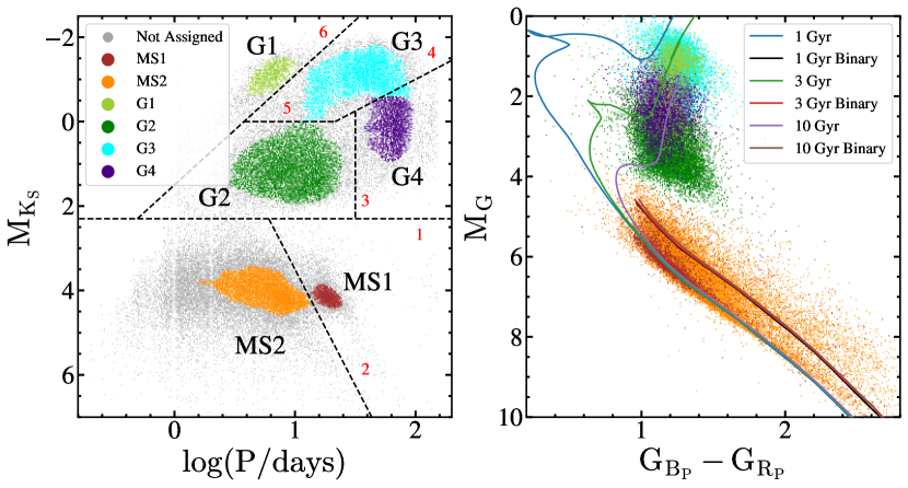
Figure 1: (Left panel) Distribution of the stars in absolute K_s magnitude and period with the clusters assigned by HDBSCAN, and the boundaries used to manually assign all the stars to groups. The dashed boundaries are numbered in red, corresponding to those in Table 1. (Right panel) Distribution of the rotational variables in absolute G magnitude versus B${}_{P}-$R_P color, color-coded by the manually assigned cluster. We also include 1, 3, and 10 Gyr Solar metalicity PARSEC isochrones (Bressan et al., 2012; Marigo et al., 2013). The main sequence is also shown at twice the luminosity as the sequence of "twin" binaries. Stars above the sequence of twin binaries are probably young stellar objects (YSOs).

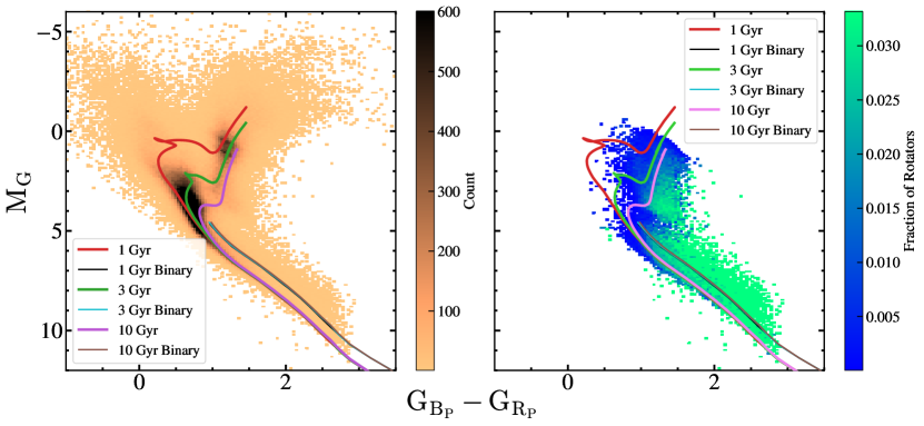
Figure 2: (Left panel) Absolute G magnitude versus $B_{P}-R_{P}$ color for a random sample of $\sim$500,000 ASAS-SN sources searched for variability where the bin color corresponds to the number of sources. (Right panel) Absolute G magnitude versus $B_{P}-R_{P}$ color where bin color corresponds to the fraction of stars which were identified as rotational variables. Both panels are overlayed with the same isochrones as in the right panel of Figure 1.

Here we consider the subsample of $48,298$ rotational variables shown in the left panel of Figure 1. We restricted the sample to systems with Gaia EDR3 (Gaia Collaboration et al., 2016, 2021) parallax signal-to-noise ratios of $>10$. We use distances from Bailer-Jones et al. (2021) and extinction estimates from the mwdust (Bovy et al., 2016) ‘Combined19’ dust map (Drimmel et al., 2003; Marshall et al., 2005; Green et al., 2019). We keep systems with estimated extinctions $A_{V}<2$ and dispose of the small number of outliers with either extinction corrected $B_{P}-R_{P}>3$ or $M_{G}<-1$. The ASAS-SN variable catalog is dominated by the V band sample (Jayasinghe et al., 2018, 2019b, 2019a, 2020, 2021) which had significant systematic problems for periods near one day, so we reject systems with $\rm{log_{10}(Period/days)}$ between $-.0018$ and $.0005$.

The left panel of Figure 1, the distribution of our sample in period and absolute 2MASS (Skrutskie et al., 2006) K_s magnitude, appears to have $6$ clusters; four of giants and two of main sequence stars. To test this more formally, we used the density-based clustering algorithm HDBSCAN (McInnes et al., 2017) to identify clusters in this parameter space. HDBSCAN assigns each source to one of the clusters or to noise. We first separated the main sequence and giants using the input parameter min_cluster_size = 1000. We further divided the main sequence using min_cluster_size = 1000 with the additional parameters min_samples = 200, and cluster_selection_epsilon = .07, and the giants using min_cluster_size = 1000, with the additional parameters min_samples = 150, and cluster_selection_epsilon = .07.

This combination of parameters lead to the identification of $7$ clusters, the $6$ identified by eye and a seventh associated with the 1 day period notch. We ignore this grouping (it is not shown in Figure 1) and assign it to the adjacent cluster. The combination of parameters we used in HDBSCAN were meant to maximize the number of points assigned to clusters, but nonetheless many of the stars were not assigned to any group, as can be seen in the left panel of Figure 1. For our analysis, we divided the stars into 6 clusters using the lines shown in the left panel of Figure 1 and presented in Table 1 to expand the HDBSCAN clusters to include all of the stars. We label these initial groups as MS1 and MS2 for the main sequence, G1 and G2 for the shorter period giants, and G3 and G4 for the longer period giants. The right panel of Figure 1 shows these clusters in extinction-corrected absolute G magnitude and B${}_{P}-$R_P color and the groups also partially separate in this space. While we begin with these six groups identified in period and absolute magnitude, we find them to further subdivide using other parameters; we will discuss this in Section 3.

We visually inspected 100 randomly selected light curves from each group. The light curves overwhelmingly are those of rotational variables with very little contamination. We had hoped that there would be some qualitative differences between the light curves of the different groups, but no such differences were apparent. The residual low-level contamination observed in the light curves and the fact that we do not expect our manual divisions to be perfect will lead to scatter in other parameter spaces. Nonetheless, these divisions suffice for our purpose of highlighting the bulk properties of each group. We also checked distributions in ASAS-SN amplitudes for each group, but the only obvious trend is the selection effect that fainter stars need higher amplitudes to be identified as variables.

Table 1: Boundaries used to separate groups (labeled in red in the left panel of Figure 1).

Boundary #	Equation	Range
1	$\rm{M_{K_{S}}=2.3}$	$\rm{-1<\log(P/days)<3}$
2	$\rm{M_{K_{S}}=5.5\log(P/days)-2}$	$\rm{0.782<\log(P/days)<3}$
3	$\rm{\log(P/days)=1.5}$	$\rm{-0.25<M_{K_{S}}<2.3}$
4	$\rm{M_{K_{S}}=-1.5\log(P/days)+2}$	$\rm{1.33<\log(P/days)<3}$
5	$\rm{M_{K_{S}}=0}$	$\rm{-0.577<\log(P/days)<1.33}$
6	$\rm{M_{K_{S}}=-2.6\log(P/days)+1.5}$	$\rm{-0.308<\log(P/days)<3}$

We also extracted 500,000 random stars from the full sample of ASAS-SN stars searched for variability in Christy et al. (2023), and the left panel of Figure 2 shows their distribution in color and absolute magnitude. The right panel shows the fraction of sources identified as rotational variables. This uses the ratio of the number of rotational variables to the number of random sources statistically corrected to be the fraction of the full input sample. This makes no attempt to determine selection effects, but there is a clear absence of rotational variables on the main sequence above the Kraft (1967) break and on the upper giant branch. Rotational variables are more common lower on the main sequence, along the binary main sequence and for the sub-subgiants (Leiner et al., 2022).

Figure 3 compares our sample in amplitude and period to the McQuillan et al. (2014) sample of rotational variables in Kepler. As a ground-based survey, ASAS-SN probes a higher-amplitude sample and over a broader period range than Kepler, which focused on a field dominated by old stars with low variability amplitudes (Brown et al., 2011). The two samples have essentially no overlap.

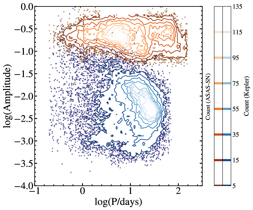
Figure 3: Distribution in amplitude and rotation period for the ASAS-SN (orange) and Kepler (blue) rotational variables from McQuillan et al. (2014). We binned the data in this parameter space and the lines show contours of constant bin count. The amplitudes are in the g-band for ASAS-SN stars and in Kepler’s bandpass for Kepler stars. Kepler (ASAS-SN) amplitudes are the 5–95% (2.5–97.5%) ranges of the light curves.

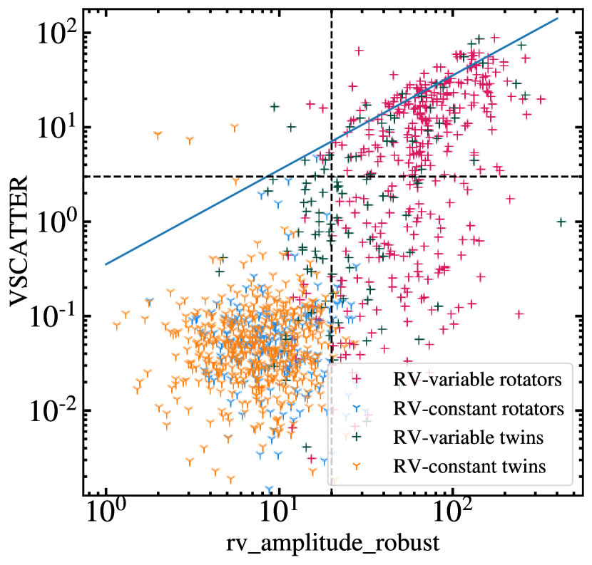
Figure 4: Comparison between APOGEE’s VSCATTER parameter and Gaia’s rv_amplitude_robust, including all rotators and twins meeting the criteria for the Gaia RV-variability analysis and with APOGEE NVISITS $>1$, and coded by whether they meet the Katz et al. (2022) criteria to be considered RV-variable. The blue diagonal indicates where VSCATTER $=\rm{\texttt{rv\_amplitude\_robust}}/2\sqrt{2}$. The vertical line indicates rv_amplitude_robust=20 km s^-1 and the horizontal line indicates VSCATTER=3 km s^-1.

We matched the rotational variables sample to APOGEE DR17 (Abdurro’uf et al., 2022) and Gaia DR3 (Gaia Collaboration et al., 2022). Table 2 displays the number of stars in each survey as well as in certain subsets, and Table 3 shows the fractions of stars in each group with characteristics derived from this ancillary data. From Gaia, we include in Table 3 the fraction of sources with RUWE $\geq$ 1.2, a conservative indicator for a wide binary or triple companion (Pearce et al., 2020; Belokurov et al., 2020), flagged astrometric binaries (7- and 9-parameter acceleration solutions and astrometric orbits) (Holl et al., 2022), spectroscopic (SB1 and SB2) binaries (Babusiaux et al., 2022), and systems with high dispersions in their Gaia radial velocities (see below). The astrometric binaries, systems with astrometric accelerations, and systems with high RUWE are all associated with long period orbits that should not be directly associated with the rotational variability. We can see this explicitly in the astrometric binaries, where the typical period is 100-1000 days. Wide binaries can, however, indirectly be associated with the rotational variability if the system is really a triple and the long period companion drives the evolution of a short period inner binary through Kozai-Lidov-type interactions (e.g., Fabrycky & Tremaine 2007). We also use the Gaia $v_{\rm{broad}}$ parameter as an estimate of the stellar rotation $v\sin i$. Based on Frémat et al. (2022), $v_{\rm{broad}}>10$ km s^-1 is indicative of fast rotation while lower values are consistent with noise. However, Patton et al. (2023) adopt the more conservative rapid rotation threshold $v_{\rm{broad}}>20$ km s^-1, which yields better agreement with their rapid rotator fractions from APOGEE $v\sin i>10$ km s^-1.

Gaia DR3 includes a number of variables which can be used to identify probable binaries through the scatter of the individual radial velocity (RV) measurements compared to the estimated noise, as described in Katz et al. (2022). We considered stars with

1. rv_nb_transits $\geq$ 5,

2. rv_expected_sig_to_noise $\geq$ 5, and

3. 3900 $\leq$ rv_template_teff $\leq$ 8000.

We found that either the rv_renormalised_gof or rv_amplitude_robust variables provided the clearest distinctions between probable binary and single (or wide binary) stars, where rv_renormalised_gof is a measure of the goodness of fit of a constant RV to the data, and rv_amplitude_robust is the peak-to-peak velocity amplitude after clipping outliers. Katz et al. (2022) use a conservative criterion for a binary of $\texttt{rv\_renormalised\_gof}>4$ and $\texttt{rv\_chisq\_pvalue}\leq 0.01$. For ease of comparison to the APOGEE VSCATTER (see below), we will focus on rv_amplitude_robust. Based either on the value of rv_renormalised_gof or the comparison to APOGEE, we find that $\texttt{rv\_amplitude\_robust}\geq 20$ km s^-1 is a good proxy for binarity. Requiring more transits (10) or higher signal-to-noise (10) had little effect on the results.

We use the stellar parameters $T_{\rm{eff}}$, $\log g$ and $v\sin i$ from the APOGEE survey. Where APOGEE has multiple RV measurements (NVISITS>1), we can use the root-mean-square scatter of the velocities VSCATTER as an indicator of binarity. Stars with VSCATTER $\geq 3$ km s^-1 (approximately equivalent to having a maximum difference in individual radial velocity measurements $\Delta RV_{\rm{max}}>$3–10 km s^-1) are almost certainly binaries (Badenes et al., 2018; Mazzola et al., 2020). We also include the number of stars with estimates of starspot coverage from the LEOPARD spectroscopic analysis of Cao & Pinsonneault (2022). This algorithm fits the APOGEE spectrum using models with two different $T_{\rm{eff}}$ to estimate a temperature difference and a spot fraction $f_{\rm{spot}}$ for the fraction of the stellar surface associated with the cooler temperatures. This analysis can also interpret SB2’s as spot contributions if the spectral types of each star are similar, which is only likely for similar mass main sequence binaries.

Table 2: Statistics of available data.

Rotators Sample	Total	MS1	MS2	G1	G2	G3	G4
All Gaia	48298	3258	20140	2342	10619	7201	4738
Viable for Gaia RV analysis	38446	2860	14951	2177	7356	6867	4235
All APOGEE	2133	221	1073	64	395	219	161
APOGEE NVISITS > 1	1438	139	711	44	273	156	115
$f_{\rm{spot}}$ Estimates	2121	219	1069	64	392	218	159
Twins Sample	Total	MS1	MS2	G1	G2	G3	G4
All Gaia	44836	3191	19665	2254	8224	6945	4557
Viable for Gaia RV analysis	36879	2857	14965	2100	6368	6559	4030
All APOGEE	1892	206	1039	66	188	238	155
APOGEE NVISITS > 1	1279	132	694	44	114	178	117
$f_{\rm{spot}}$ Estimates	1873	203	1025	66	186	238	155

Table 3: Fractions of stars in each group with the characteristics listed in the left column. Fractions are for the subsample in Table 2 for which the measurement exists.

Rotators Sample	MS1	MS2	G1	G2	G3	G4
Gaia RUWE $\geq$ 1.2	43.0%	35.0%	9.8%	12.2%	12.4%	12.6%
Gaia Astrometric Binaries	4.3%	3.5%	0.5%	0.5%	0.3%	0.7%
Gaia Spectroscopic Binaries	1.0%	0.8%	3.5%	1.4%	14.0%	9.9%
Gaia Variable Radial Velocity	13.9%	58.6%	98.4%	94.8%	87.1%	58.8%
rv_amplitude_robust$\geq 20$ km s-1	13.3%	58.4%	97.1%	94.3%	79.7%	51.9%
APOGEE VSCATTER $\geq$ 3 km s-1	4.3%	34.3%	86.4%	85.0%	73.7%	63.5%
Twin Sample	MS1	MS2	G1	G2	G3	G4
Gaia RUWE $\geq$ 1.2	38.0%	43.1%	11.6%	15.4%	12.8%	14.6%
Gaia Astrometric Binaries	5.3%	6.3%	0.3%	1.2%	0.6%	1.2%
Gaia Spectroscopic Binaries	1.4%	0.7%	1.3%	0.8%	1.7%	1.5%
Gaia Variable Radial Velocity	14.7%	26.3%	11.5%	16.3%	10.6%	13.7%
rv_amplitude_robust$\geq 20$ km s-1	13.7%	27.0%	6.4%	16.5%	5.3%	9.9%
APOGEE VSCATTER $\geq$ 3 km s-1	10.6%	11.2%	4.6%	10.5%	1.7%	7.7%

To explore how the rotational variables compared to similar stars which are not known rotators, we constructed a sample of twins. For each star we selected all Gaia stars with

1. a parallax within 0.9 and 1.1 times the parallax of the rotator,

2. a difference in G magnitude less than $0.025n$,

3. a difference in B_P magnitude less than $0.025n$, and

4. a difference in R_P magnitude less than $0.025n$,

where $n$ is an integer starting at $n=1$. We assign each star a metric which is simply the unweighted quadrature sum of the differences in parallax, $G$, $B_{P}$, and $R_{P}$ magnitudes and keep the lowest 16. If we find fewer than 16 stars, we iteratively increase $n$ until we have 16 stars. In most cases we succeed with $n=1$ and the overwhelming majority succeed for $n\leq 2$. We then get the mwdust extinction estimates for all 16 candidates and keep the one whose extinction is closest to the extinction of the rotator. We finally use the $\sim$93% of twins whose extinctions agree to $|\Delta A_{V}|\leq 0.2$ mag, which means that the extinction-corrected magnitudes and colors will have maximum differences due to the extinction mismatch of 0.2 and 0.1 mag, respectively. By keeping more than 16 candidates we could still better match the extinctions, but this seemed good enough for our purposes given the small discrepancies in extinction-corrected photometry. We then extracted all of the ancillary data for the twins that we obtained for the rotators. For all of the rotator classes except G2 this provided twins for $\simeq 97\%$ of the stars, while for G2 we are left with twins for only 77% of the stars. Much of the G2 group lies brighter than the main sequence but redwards of the red giant branch. Such sub-subgiants are relatively rare, so it is not surprising that it is more difficult to find twins.

The extinction-corrected absolute magnitude and color distributions of the twins and their corresponding rotational variables are very similar, as are their Gaia $\log g$ and $T_{\rm{eff}}$ distributions. The APOGEE $\log g$ and $T_{\rm{eff}}$ distributions show several notable differences as can be seen from the summary statistics in Table 4. The two MS samples are fairly similar, although the MS2 $T_{\rm{eff}}$ distribution of the twins extends to modestly (a few $100$ K) hotter temperatures. There are clear shifts for all of the giant groups, where the twins have systematically higher $T_{\rm{eff}}$ and lower $\log g$ than their corresponding rotators. This is a known bias in the APOGEE parameters for active stars: APOGEE’s analysis pipeline does not include rotation as a free parameter when fitting giant spectral templates, so the broadening of the lines created by spots and rotation in rapidly rotating giants strongly influence the derived stellar parameters, leading to underestimates of effective temperature and overestimates of surface gravity (Patton et al., 2023).

Table 4: Median APOGEE $\log g$ and $T_{\rm{eff}}$ for each group of rotators and its twin sample, with 16^th and 84^th percentile uncertainties.

	$\log g$	$T_{\rm{eff}}$ (K)
MS1 rotators	$4.57^{+0.03}_{-0.05}$	$4735^{+233}_{-437}$
MS1 twins	$4.57^{+0.03}_{-0.04}$	$4748^{+224}_{-364}$
MS2 rotators	$4.57^{+0.07}_{-0.16}$	$4234^{+427}_{-390}$
MS2 twins	$4.59^{+0.05}_{-0.05}$	$4431^{+375}_{-538}$
G1 rotators	$2.74^{+0.19}_{-0.13}$	$4616^{+47}_{-77}$
G1 twins	$2.61^{+0.34}_{-0.19}$	$4692^{+149}_{-106}$
G2 rotators	$3.57^{+0.36}_{-0.28}$	$4435^{+197}_{-233}$
G2 twins	$3.42^{+0.27}_{-0.21}$	$4901^{+156}_{-165}$
G3 rotators	$2.99^{+0.21}_{-0.30}$	$4560^{+106}_{-121}$
G3 twins	$2.61^{+0.25}_{-0.14}$	$4692^{+162}_{-120}$
G4 rotators	$3.30^{+0.23}_{-0.16}$	$4682^{+321}_{-160}$
G4 twins	$3.12^{+0.26}_{-0.26}$	$4821^{+162}_{-131}$

Figure 4 compares the APOGEE VSCATTER to the Gaia rv_amplitude_robust for both the twins and the rotators. The points are coded by whether they meet the Katz et al. (2022) criteria for RV variability. For a sine wave, the radial velocity amplitude rv_amplitude_robust would be $2\sqrt{2}$ larger than VSCATTER. The two estimates of velocity scatter are reasonably well correlated, but the overall scatter is large because both are based on a small (APOGEE) or modest (Gaia) number of measurements. Nonetheless, rv_amplitude_robust>20 km s^-1 is a reasonable proxy for binarity.

3 Discussion

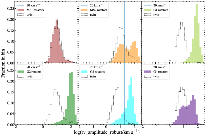
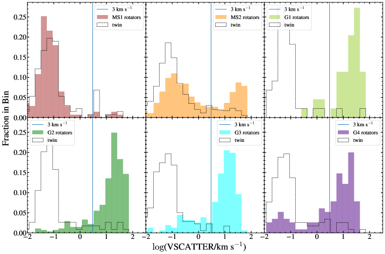
Figure 5: Distributions of each group of rotators and their twins in Gaia rv_amplitude_robust (top) and in APOGEE VSCATTER (bottom). Stars to the right of the vertical lines at $20$ km/s (Gaia) and $3$ km/s (APOGEE) are almost certainly binaries.

We expect binarity to play a key role in producing rotational variables, so we start with the distributions in Gaia rv_amplitude_robust and APOGEE VSCATTER, shown for each group and its twin in Figure 5. We see that the MS1 distribution is single-peaked at low rv_amplitude_robust and VSCATTER, with a nearly identical distribution to its twins, and so MS1 consists largely of single stars (or sufficiently wide binaries). The rotators in MS2 are strongly bimodal with one group of single stars and one group of binaries which we label MS2s and MS2b, respectively. In the right panel of Figure 1, we see that the MS2 group lies both on the main sequence (MS2s) and on the "binary main sequence," above the main sequence in magnitude where the luminosities of the PARSEC isochrones have been doubled (MS2b). The MS2 twins also show a significant tail of RV variables, almost certainly because twins of MS2b stars on the binary main sequence are also binaries.

Separating MS2s/b based only on radial velocity scatter yields a small sample, limited to stars with multiple radial velocity measurements, but we can also divide MS2 photometrically. We use the criteria from Cao & Pinsonneault (2022), who fit a polynomial to the observed main sequence and defined photometric binaries as those at least 0.25 mag brighter than this fit. This method implies a binary fraction for MS2 of $\sim 43\%$. For comparison, if we just split the APOGEE VSCATTER sample at 3 km s^-1, we would have a binary fraction of $\sim 34$%. Since this is incomplete because it does not account for binaries missed due to inclination, the two estimates are reasonably consistent. We use the photometric division of MS2s/b in §4 when comparing our main sequence sample to that of McQuillan et al. (2014).

To compare the results of separating MS2s/b photometrically and based on radial velocity scatter, Figure 6 shows a color-magnitude diagram of MS2 stars colored by whether VSCATTER$\geq 3$ km s^-1. We see a band of low-VSCATTER stars on the main sequence, a band of high-VSCATTER stars on the binary main sequence, and a third band of low-VSCATTER stars above the binary main sequence. This upper band of stars with low RV scatter is not present in color-magnitude diagrams where we split instead by whether rv_amplitude_robust$\geq 20$ km s^-1, or based on RV variability according to criteria from Katz et al. (2022). Unresolved triple systems could lie above the binary main sequence without having significant radial velocity scatter, but we saw no indication in Gaia RUWE that this upper band of low-VSCATTER stars are triple systems. Instead, these are probably young stellar objects (YSOs), which also have quasi-periodic rotational modulation, but lie well above the main sequence (Rebull et al., 2016). To confirm this, we verified that that the YSO candidates have higher than average $A_{V}$.

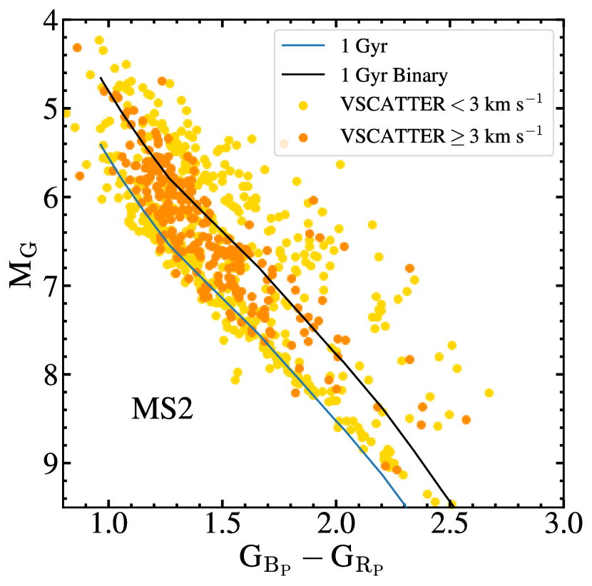
Figure 6: Absolute G magnitude versus $\rm{B_{P}-R_{P}}$ color for MS2 stars with valid VSCATTER measurements with the single and binary 1 Gyr PARSEC isochrones from Figure 1 overlayed.

The G1-G3 rotators are all clearly binaries based on their rv_amplitude_robust and VSCATTER distributions, whereas their twins are predominantly single stars. While the G4 twins are overwhelmingly single, the G4 distribution is bimodal, indicating subpopulations of both single (G4s) and binary (G4b) stars. Note that the bimodality seen in MS2 and G4 is real and not due to inclination. Inclination effects produce distributions with the rapidly dropping tails to lower velocity seen for G3. Formally, for a true binary of orbital velocity $v_{T}$, the observed velocity $v_{0}$ is distributed as $x(1-x^{2})^{-1/2}$, with $x=v_{0}/v_{T}$ for a uniform distribution in $\cos i$. The single star subset of G4 likely consists of merger products. The distributions in Gaia rv_renormalised_gof confirm the results of the rv_amplitude_robust and VSCATTER distributions, in particular the existence of the G4 merger subpopulation.

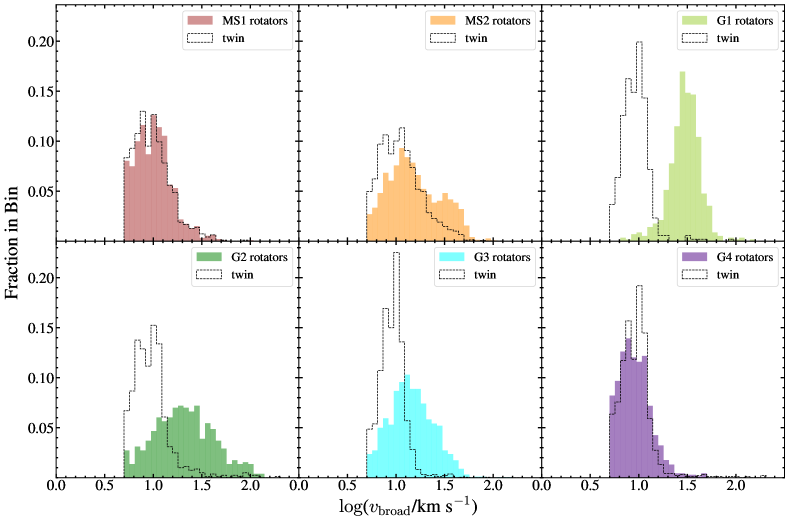
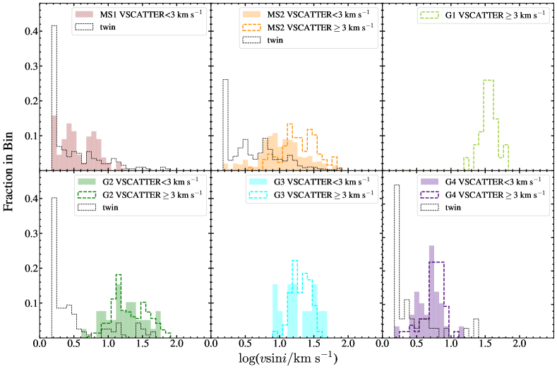
Figure 7: Distributions in $v_{\rm{broad}}$ (top) and $v\sin i$ (bottom) for each group and their twins. The $v\sin i$ distributions are split by VSCATTER, where the solid histograms are for VSCATTER<3 and the dashed histograms are for VSCATTER$\geq$3 km s^-1. The G1 and G3 twins, as well as the high-VSCATTER population of MS1 and low-VSCATTER population of G1 have $<10$ APOGEE $v\sin i$ measurements and are not shown because there are too few systems.

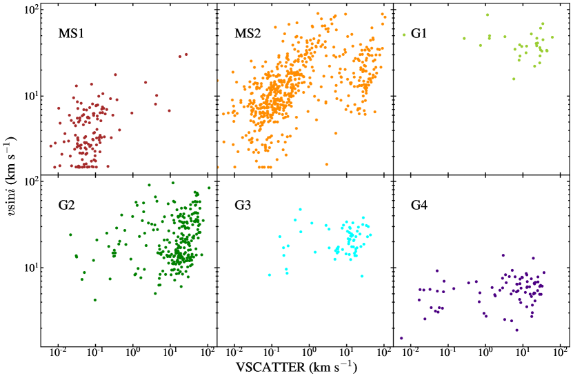
Figure 8: Distributions in APOGEE $v\sin i$ and VSCATTER for each group.

We also expect rotation rates to be an important physical probe of rotational variables, and Figure 7 shows the twin and rotator distributions in APOGEE $v\sin i$ and Gaia $v_{\rm{broad}}$, as an estimator of $v\sin i$. The $v\sin i$ distributions include only stars with NVISITS>1 and are split by whether VSCATTER$\geq 3$ km s^-1. The median $v\sin i$ values for each subgroup are given in Table 5. While the APOGEE $v\sin i$ should be accurate even for small velocities, comparisons with APOGEE show that values of Gaia $v_{\rm{broad}}<10$ km s^-1 should be regarded as upper limits (Frémat et al., 2022). MS1, and its twin are comprised of slow rotators. In Table 5, we see that the high VSCATTER stars of MS1 have a much higher median $v\sin i$, but the small number of them means that they are not included in Figure 7. MS2, particularly in $v_{\rm{broad}}$, again seems bimodal, while its twin is comprised predominantly of slower rotators. In Figure 8, where we show the distribution of MS1 and MS2 in both VSCATTER and $v\sin i$, there is a clear separation of MS2 into two populations, where the high-VSCATTER systems all have high $v\sin i$. MS2’s bimodality is less obvious in the $v\sin i$ distributions because there are low-VSCATTER systems with high $v\sin i$. The slower MS2 rotators still seem to have larger $v\sin i$ than the MS2 twins and MS1.

The giants are in three groups. G1 has high $v\sin i$ and $v_{\rm{broad}}$, and while its twin group has very few $v\sin i$ measurements, it tends to have lower $v_{\rm{broad}}$. G4 has the slowest rotation rates of the giants, and while it has a similar $v_{\rm{broad}}$ distribution to its twin, the G4 twins have still slower $v\sin i$. Of the giant groups, G4 is the only one where the high-VSCATTER stars do not have a high $v\sin i$. The G4 stars have long rotational periods, so the smaller $v\sin i$ are expected, but the cause is physically interesting. The G4 binary stars are not tidally locked, but are in sub-synchronous orbits (see the discussion associated with Figure 10). G2 and G3 have intermediate rotation rates to G1 and G4, and their twins tend to have slower rotation rates (though the G3 twins have very few $v\sin i$ measurements). Note that because of the crudeness of the $v_{\rm{broad}}$ parameter, the Gaia equivalent of Figure 8, $v_{\rm{broad}}$ versus rv_amplitude_robust, is uninformative.

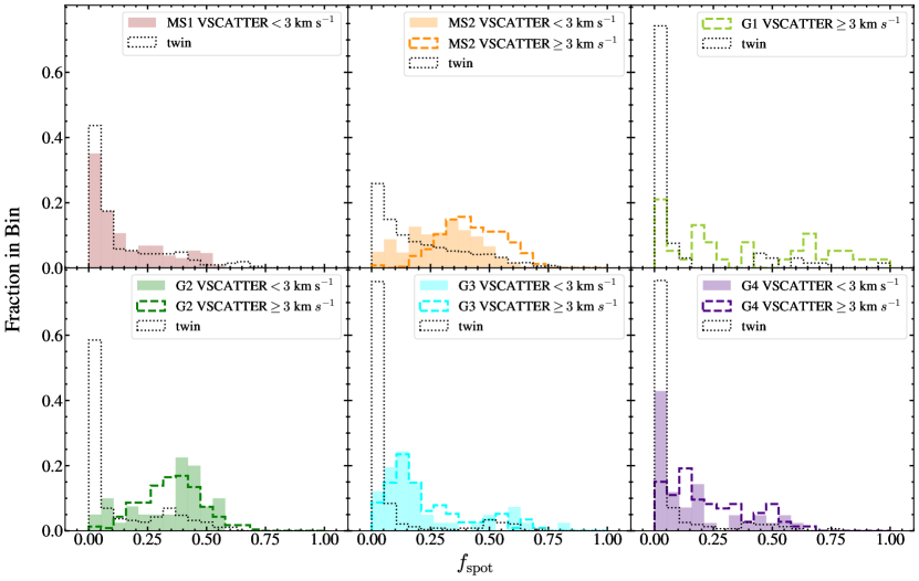
Figure 9: Distributions of the spot fraction $f_{\rm{spot}}$ for each group. The solid histograms are for rotational variables with APOGEE VSCATTER < 3 km s^-1 and the colorful dashed histograms are distributions for stars with VSCATTER$\geq$3 km s^-1. The black dashed histograms are for the twin groups. Only distributions with $\geq 10$ members are shown.

Figure 9 shows the distributions of the stars in the starspot filling fraction ($f_{\rm{spot}}$) where the rotational variables are also divided into likely binaries with $\texttt{VSCATTER}\geq 3$ and likely non-binaries with $\texttt{VSCATTER}<3$. Cases when there are fewer than $10$ stars are not shown. Table 5 gives the median spot fractions of each group. Except for the MS2 twins, the twin populations have $f_{\rm{spot}}$ distributions strongly peaked near zero. It seems likely that many of the tails of the twin distributions towards higher spot fractions are due to the presence of spotted stars which have not been recognized as rotational variables.

The spot fractions are estimated from the individual APOGEE epochs, and so are unaffected by the presence of orbital Doppler shifts, but they can be affected by the presence of spectral contamination from the companion. This means that only the main sequence binary sub-population MS2b, which tends to lie close to the binary main sequence, can have significant biases in $f_{\rm{spot}}$ due to the presence of a binary companion. The giant binaries will generally have a much lower luminosity main sequence companion which cannot significantly contaminate the giant’s spectrum.

MS1 contains few binaries and has a spot fraction distribution nearly identical to its twins. There is, however, a modest binary sub-population that is more heavily spotted (see Table 5). MS2 has significantly higher spot fractions than its twins, and the non-binary MS2s sub-sample is modestly less spotted than the binary MS2b sub-sample. The MS2s stars are, however, much more spotted than the MS1 stars supporting the argument than they are two different populations rather than a continuum. Here the long tail on the twin distribution is due to the tendency of MS2b twins to also be binaries. We confirmed that the high-$f_{\rm{spot}}$ MS2 twins also tend to have high VSCATTER.

G1 has a very broad range of spot fractions, although the median of $f_{\rm{spot}}\sim 28\%$ is less than that of the MS2 and G2 groups and similar to that of the MS1 group. Except for the likely merger sub-population of G4, the spotted giants are all binaries based on their VSCATTER distributions. This means that the low-VSCATTER systems should be dominated by binaries viewed at high inclinations rather than being a physically distinct population, so we expect similar spot fractions at high- and low-VSCATTER for G1, G2 and G3 but not G4, as we see in Figure 9 and Table 5. The G2 group has the highest median spot fractions with the low-VSCATTER group having a modestly higher median ($f_{\rm{spot}}\simeq 40\%$ versus $36\%$). The G3 group has some of the lowest spot fractions with little difference between the high- and low-VSCATTER sub-samples. Like G2, the VSCATTER distributions again argue for a purely binary population. Finally, the G4 group has some of the lowest spot fractions, but the high-VSCATTER systems are significantly more spotted than the low-VSCATTER systems. Unlike G1, G2, and G3, G4 does have a large number of non-binary, low-VSCATTER systems, so it is not surprising that they also have different spot fractions.

Table 5: Median $f_{\rm{spot}}$, $v\sin i$, $v_{\rm{broad}}$, $P_{\rm{rot}}$, and $P_{\rm{orb}}$ of each group and their twin as a whole, and each group of rotators separated by whether VSCATTER$\geq 3$ km s^-1 (for stars with >1 APOGEE visit) or whether rv_amplitude_robust$\geq 20$ km s^-1 (for stars meeting the criteria for Gaia radial velocity analysis outlined in Section 2). For some subsets, there were no stars with orbital period estimates from Gaia, so their $P_{\rm{orb}}$ entries are left blank. Stars from the "twin" sample are not ASAS-SN rotational variables and do not have ASAS-SN rotational periods, so their $P_{\rm{rot}}$ entries are marked "n/a."

median:	$f_{\rm{spot}}$	$v\sin i$ (km/s)	$v_{\rm{broad}}$ (km/s)	$P_{\rm{rot}}$ (days)	$P_{\rm{orb}}$ (days)
All MS1 Rotators	0.09	3.4	9.9	18.1	13.9
MS1 VSCATTER$<3$ km s-1	0.09	3.3	9.4	18.1
MS1 VSCATTER$\geq 3$ km s-1	0.28	10.2	24.5	12.7
MS1 rv_amplitude_robust$<20$ km s-1	0.06	2.7	9.8	18.5	180.6
MS1 rv_amplitude_robust$\geq 20$ km s-1	0.27	7.7	12.2	16.7	14.1
MS1 twins	0.06	2.2	9.3	n/a	25.3
All MS2 Rotators	0.35	12.8	14.1	3.7	6.1
MS2 VSCATTER$<3$ km s-1	0.30	10.6	15.0	5.0
MS2 VSCATTER$\geq 3$ km s-1	0.41	20.2	15.0	2.3	6.1
MS2 rv_amplitude_robust$<20$ km s-1	0.17	6.6	11.9	8.5	4.0
MS2 rv_amplitude_robust$\geq 20$ km s-1	0.37	16.5	20.2	3.3	6.1
MS2 twins	0.14	3.6	10.7	n/a	23.8
All G1 Rotators	0.24	37.8	30.2	5.4	13.4
G1 VSCATTER$<3$ km s-1	0.27	48.1	41.5	7.9
G1 VSCATTER$\geq 3$ km s-1	0.28	36.3	32.3	5.2	9.6
G1 rv_amplitude_robust$<20$ km s-1	0.31	48.7	34.3	10.2
G1 rv_amplitude_robust$\geq 20$ km s-1	0.16	37.8	30.0	5.8	13.4
G1 twins	0.01	2.2	9.2	n/a	240.6
All G2 Rotators	0.37	20.0	20.3	9.0	12.4
G2 VSCATTER$<3$ km s-1	0.40	18.1	13.2	8.1
G2 VSCATTER$\geq 3$ km s-1	0.36	19.2	27.1	9.0	13.1
G2 rv_amplitude_robust$<20$ km s-1	0.15	8.5	11.6	23.5	695.2
G2 rv_amplitude_robust$\geq 20$ km s-1	0.35	19.7	21.1	9.0	12.3
G2 twins	0.02	2.1	9.1	n/a	35.7
All G3 Rotators	0.15	21.3	14.0	30.9	41.1
G3 VSCATTER$<3$ km s-1	0.14	17.9	13.3	41.9	48.9
G3 VSCATTER$\geq 3$ km s-1	0.16	21.2	17.0	29.4	36.0
G3 rv_amplitude_robust$<20$ km s-1	0.13	15.2	11.7	49.3	45.4
G3 rv_amplitude_robust$\geq 20$ km s-1	0.14	23.2	14.8	32.0	41.1
G3 twins	0.01	20.0	9.3	n/a	352.7
All G4 Rotators	0.13	5.4	9.0	64.4	28.9
G4 VSCATTER$<3$ km s-1	0.10	5.3	9.5	64.9	26.2
G4 VSCATTER$\geq 3$ km s-1	0.17	6.0	7.2	59.8	36.9
G4 rv_amplitude_robust$<20$ km s-1	0.01	3.5	8.9	74.8	17.4
G4 rv_amplitude_robust$\geq 20$ km s-1	0.14	5.8	9.0	66.8	29.7
G4 twins	0.00	1.9	9.1	n/a	175.5

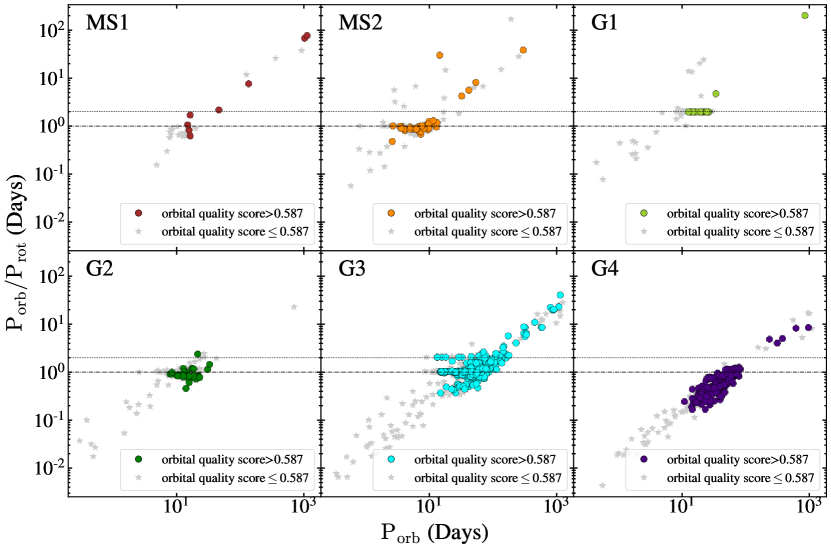
Figure 10: Ratio of the Gaia SB1 $P_{\rm{orb}}$ to the ASAS-SN $P_{\rm{rot}}$ versus $P_{\rm{orb}}$. The lower dashed line is for $P_{\rm{orb}}=P_{\rm{rot}}$ and the upper dotted line is for $P_{\rm{orb}}=2P_{\rm{rot}}$. The colorful points have orbital scores $>0.587$ and the grey background points have orbital scores $\leq 0.587$.

Figure 10 shows the ratio of the Gaia SB1 orbital period, $P_{\rm{orb}}$, to the ASAS-SN rotational period, $P_{\rm{rot}}$, as a function of $P_{\rm{orb}}$ for each group. We expect many rotational variables to be tidally synchronized binaries so we include lines at $P_{\rm{orb}}=P_{\rm{rot}}$ and $P_{\rm{orb}}=2P_{\rm{rot}}$. There is no physics that would yield the $P_{\rm{orb}}=2P_{\rm{rot}}$ ratio, but it is difficult to measure an orbital period to be half it’s actual value. Therefore, rotators lying on this line likely have a reported rotational period aliased to half the true value (see below).

Many of the widely-scattered points are likely due to incorrect Gaia periods (Jayasinghe et al. 2022 found for $\sim 11$% of their detached eclipsing binary sample that the orbital periods from Gaia SB1 disagreed with values from ASAS-SN). To verify this, we used orbital score values from Bashi et al. (2022) assigned to each Gaia SB1, where the score (ranging from 0 to 1) corresponds to the validity of the orbital solution. They recommend a "clean score limit" of $0.587$, which yields a sensitivity of 80% (that is, a sample of SB1’s with scores $>0.587$ should have fewer than 20% false orbits). Figure 10 separates each group by whether their score is $>0.587$. For most groups, the systems with higher scores lie overwhelmingly on one of the horizontal lines, while the systems with lower scores account for a majority of the scatter. Additionally, we assume that systems with reliable Gaia periods also have reliable Gaia eccentricities, and expect the spectroscopic binaries in our sample to be in close circular orbits after tidal synchronization. Most of the non-synchronous systems are also reported to be eccentric ($e>0.1$).

MS1 tends to have somewhat shorter $P_{\rm{orb}}$ than $P_{\rm{rot}}$ and MS2 tends to be synchronized. G1 is strongly clustered on $P_{\rm{orb}}=2P_{\rm{rot}}$. While this is typical of ellipsoidal variables and contact binaries, our visual inspection of the light curves rules out misclassification of such stars. Instead, G1 likely consists of rotators in synchronized binaries with two dominant and roughly symmetrically-placed starspots such that the frequency of their observed change in brightness is doubled compared to their actual rotation period. G2 is strongly clustered on $P_{\rm{orb}}=P_{\rm{rot}}$ and so consists of synchronized systems. G3 also consists largely of stars with $P_{\rm{orb}}=P_{\rm{rot}}$. G3 systems with low orbital scores and non-zero eccentricity contribute significant scatter, especially for $P_{\rm{orb}}>P_{\rm{rot}}$. The G4b systems with both reliable and unreliable periods are strongly clustered at $P_{\rm{orb}}<P_{\rm{rot}}$, which means that G4b consists of younger giants in the process of tidal synchronization with their companions ("subsynchronous binaries"). This is consistent with the high-VSCATTER population of G4 having the lowest median $v\sin i$ of all the high-VSCATTER rotators in Table 5.

We also checked the number of stars with RUWE $\geq$ 1.2 and the number of Gaia astrometric binaries within each group. High RUWE and astrometric binaries are fairly common in the main sequence groups, but, as shown in Table 3, there is little difference in the fractions with RUWE $\geq$ 1.2 or in the fractions of flagged astrometric binaries between the rotators and their twins. High RUWE and astrometric binaries are uncommon for all giant groups and their twins, as is expected given that they are generally more distant than the main sequence sample. Overall, the presence of a widely orbiting companion or tertiary seems to be unimportant in creating rotational variables.

4 Conclusions

Based on these results, we hypothesize that we have seven distinct groups of rotational variables: MS1, MS2s, MS2b, G1/G3, G2, G4s and G4b. We summarize our major findings about each group below:

1. MS1 consists of main sequence K-M dwarfs with typical masses of $0.6$ to $0.8M_{\odot}$ based on the PARSEC isochrones. They generally are not (detectable) binaries, which for APOGEE means that the can only be in binaries with periods $>10^{3}$ days (see Mazzola et al. 2020). That they generally lie close to the main sequence means that few can have similar mass companions of any period unless they are sufficiently separated to be a spatially resolved binary. They rotate relatively slowly (median period of 18.12 days), although not quite as slowly as their APOGEE twins. The majority are not very heavily spotted.

2. MS2s also consists of main sequence stars but with masses extending from the bottom of the main sequence to $0.8M_{\odot}$. They are also not binaries up to the same caveats as for MS1. They have faster rotation periods (median period of 8.08 days) and this is reflected in the different $v\sin i$ distributions. They also have higher spot fractions.

3. The properties of MS1 and MS2s are sufficiently disjoint that we are reasonably confident they are distinct. Figure 11 shows the distribution of MS1, MS2s, MS2b, and the Kepler sample of rotational variables from McQuillan et al. (2014) in rotation period and $T_{\rm{eff}}$. In this figure, we have separated MS2s from MS2b photometrically, as described in Section 3, to maximize the sample size. The Kepler sample notably bifurcates in rotation period at $T_{\rm{eff}}<4500$K, possibly due to a transient phase of rapid mass-dependent spin-down across the gap (McQuillan et al., 2014). MS1 and MS2s seem to follow the direction of this "McQuillan gap," and while the MS2s stars span a wide range of temperatures, MS1 stars lie only at higher temperatures where McQuillan et al. (2014) did not find a bimodality in the Kepler period distribution.

   The origin of the restricted temperature or mass range of MS1 as compared to MS2 is not presently clear. One possibility is that it is simply an amplitude-dependent selection effect against cool, long-period rotators, but a completeness study of the ASAS-SN sample is a major undertaking beyond the scope of this work. That they appear to lie on an extension of the McQuillan et al. (2014) period gap suggests that one difference between MS1 and MS2s is age, but we have no direct means of testing this other than the standard gyrochronological assessment.

   

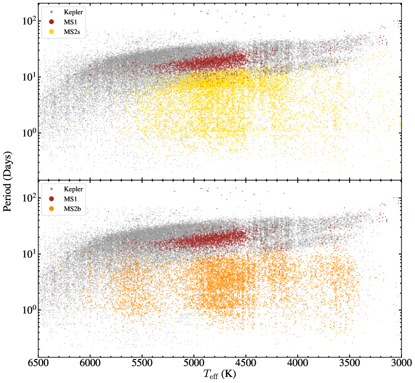
   Figure 11: Distribution of the Kepler rotational variables from McQuillan et al. (2014), MS1, MS2s (top) and MS2b (bottom) in period and $T_{\rm{eff}}$.

4. MS2b clearly is a different population than MS1 or MS2s. They are overwhelmingly synchronous binaries and many lie near the binary main sequence, indicating that the companion is of similar mass. Like the MS2s population, they seem to span the full dwarf mass range. They rotate a little faster than the MS2s stars, and have higher estimated spot filling fractions. In this case, however, the spectrum of the companion star may be contributing to the inferred spot fraction. That most of the MS2b stars have short periods suggests that the scatter of Kepler stars to similar periods is also dominated by binaries, consistent with the findings in Simonian et al. (2019).

5. We suspect that G1 and G3 are really a single group of heavily spotted red giants in synchronized binaries (which we label G1/3 going forward). The G1 systems all have $P_{\rm{orb}}/P_{\rm{rot}}=2$ (see Figure 10), which means that the true rotational period is twice that reported. If we shift G1 in rotational period, they largely overlap with G3, and they have very similar luminosities, temperatures and gravities. The are not, however, truly identical after correcting the rotation period. The G1 stars are more heavily spotted (median $f_{\rm{spot}}$ of 28% versus 16%) and have larger rotation velocities (median $v\sin i$ of 38 versus 21 km/s). Since the rotational periods are similar, the higher $v\sin i$ suggests that the G1 stars are probably viewed more edge on. G1/3 stars are likely RS CVn stars (Hall, 1976). Leiner et al. (2022) noted that the rotation periods of RS CVn lie between 1-100 days and with magnitudes $-1<M_{G}<5$, both consistent with our sample of G1/3 stars.

6. The G2 group likely consists of sub-subgiants (SSGs). Leiner et al. (2022) found SSGs to have rotation periods overwhelmingly $<20$ days, consistent with our G2 sample, and with $3<M_{G}<5$. The G2 sample spans a somewhat broader range of $2<M_{G}<5$. Leiner et al. (2022) also noted that their total RS CVn and SSG sample had increasing luminosity with rotation period, due to the necessity of a more massive companion to maintain tidal interaction in wider systems. In the left panel of Figure 1 we see a similar upward trend in the G1/3 and G2 groups. Finally, Leiner et al. (2022) suggests a limit of $P\lesssim 30$ days as a tidal circularization period for SSGs and the least luminous RS CVn, consistent with our boundary between the G2 and G4 groups (boundary #3 in Table 1) at a period of $10^{1.5}\simeq 30$ days.

7. The G4s stars with low radial velocity scatter are likely recent merger products.

8. The G4b stars with high radial velocity scatter are sub-synchronous binaries (Figure 10), beginning to tidally interact as they expand toward their companion. They are of intermediate luminosity (and so have intermediate evolution timescales) compared to G1/3 and G2, but have sufficiently wide orbits that their spin-up timescales are shorter than their evolutionary timescales. Neither the G4s recent mergers nor the G4b sub-synchronous binaries seem to have been previously recognized.

There is enormous scope for expanding on this population study of rotational variables. First, the ASAS-SN sample itself has considerable room for growth since the current sample is largely based on the older V-band ASAS-SN data and a small portion of the newer g-band data. With the additional data it should not only be possible to expand the sample considerably but it should also be possible to push to lower amplitudes. Rotational variables from brighter surveys like ASAS (Pojmanski, 2002) or KELT (Oelkers et al., 2018) could also be added, as well as the lower amplitude systems found by Kepler (e.g. McQuillan et al. 2014) or TESS (Ricker et al., 2014). Except for the well-studied Kepler field, there is less reason to expand to fainter stars because these will generally lack the ancillary spectroscopic data needed to study rotation rates, binarity, or composition. The biggest immediate return is likely from including brighter systems, since this should significantly increase the numbers of systems with Gaia spectroscopic orbits, the area of comparison where our samples are smallest.

Many of our conclusions rely primarily on the availability of APOGEE parameters, namely, VSCATTER, $v\sin i$, and $f_{\rm{spot}}$. APOGEE had specific targeting criterion which could bias our results, but we believe we cover any such biases both through confirming our observations in APOGEE data, if with lower precision, with information from Gaia, and through comparison with the twin sample. APOGEE targeting was based on photometry (Majewski et al., 2017), so comparisons with the twins should be independent of APOGEE targeting choices.

Additionally, APOGEE’s spectroscopic data is significantly limited in availability compared to the size of our initial sample (APOGEE includes only $\sim 4.4$% of the ASAS-SN rotational variables from this work). However, the numbers of stars with ancillary spectroscopic data will rapidly increase with the SDSS Milky Way Mapper (Kollmeier et al., 2017) extension of the APOGEE survey (Majewski et al., 2017) and Gaia DR4. The sources of the spectroscopic data could also be expanded to include surveys such as LAMOST (Cui et al., 2012) and DESI (Cooper et al., 2022; DESI Collaboration et al., 2022). The biggest impact will likely be Gaia DR4 because it will provide a huge expansion of the numbers of systems with spectroscopic orbits and provide the actual RV measurements, which are needed to understand many of the rejected orbital solutions from DR3. In particular, there are suggestions from Figure 10 that the G2 group might be slightly sub-synchronous, that the G3 group is a mixture of synchronized and unsynchronized systems, and that the sub-synchronous rotation of the G4b group is correlated with period. For now, we conservatively call the G2 and G3 groups synchronized, but with better orbital solutions we may find that the situation is more complex.

We also did not explore the compositions of the variables both between the groups and with their twins. The underlying reason is that APOGEE does not include stellar rotation in its models of the giants for computational reasons (Holtzman et al., 2018). This leads to biases on the inferred parameters because the broader lines created by the rapid rotation are interpreted as some other physics. We see this here in the temperature and $\log g$ offsets between the giant groups and their twins. However, this problem also biases the abundances, and Patton et al. (2023) find that apparent abundance anomalies are a means of flagging rapidly rotating APOGEE giants. Trying to understand how this problem would affect any elemental comparison seemed beyond the scope of this paper. This issue might also be one reason to include information from the large, lower resolution spectroscopic surveys like LAMOST and DESI, where the line broadening in giants due to rotation would be irrelevant.

Data Availability

All data used in this study are public.

References

- Abdurro’uf et al. (2022) Abdurro’uf et al., 2022, ApJS, 259, 35
- Andronov et al. (2006) Andronov N., Pinsonneault M. H., Terndrup D. M., 2006, ApJ, 646, 1160
- Babusiaux et al. (2022) Babusiaux C., et al., 2022, arXiv e-prints, p. arXiv:2206.05989
- Badenes et al. (2018) Badenes C., et al., 2018, ApJ, 854, 147
- Bailer-Jones et al. (2021) Bailer-Jones C. A. L., Rybizki J., Fouesneau M., Demleitner M., Andrae R., 2021, AJ, 161, 147
- Barnes (2007) Barnes S. A., 2007, ApJ, 669, 1167
- Bashi et al. (2022) Bashi D., Shahaf S., Mazeh T., Faigler S., Dong S., El-Badry K., Rix H. W., Jorissen A., 2022, MNRAS, 517, 3888
- Belokurov et al. (2020) Belokurov V., et al., 2020, MNRAS, 496, 1922
- Borucki et al. (2010) Borucki W. J., et al., 2010, Science, 327, 977
- Bouma et al. (2023) Bouma L. G., Palumbo E. K., Hillenbrand L. A., 2023, ApJ, 947, L3
- Bovy et al. (2016) Bovy J., Rix H.-W., Green G. M., Schlafly E. F., Finkbeiner D. P., 2016, ApJ, 818, 130
- Bressan et al. (2012) Bressan A., Marigo P., Girardi L., Salasnich B., Dal Cero C., Rubele S., Nanni A., 2012, MNRAS, 427, 127
- Brown et al. (2011) Brown T. M., Latham D. W., Everett M. E., Esquerdo G. A., 2011, AJ, 142, 112
- Cao & Pinsonneault (2022) Cao L., Pinsonneault M. H., 2022, MNRAS,
- Cao et al. (2023) Cao L., Pinsonneault M. H., van Saders J. L., 2023, arXiv e-prints, p. arXiv:2301.07716
- Carlberg et al. (2011) Carlberg J. K., Majewski S. R., Patterson R. J., Bizyaev D., Smith V. V., Cunha K., 2011, ApJ, 732, 39
- Ceillier et al. (2017) Ceillier T., et al., 2017, A&A, 605, A111
- Christy et al. (2023) Christy C. T., et al., 2023, MNRAS, 519, 5271
- Cooper et al. (2022) Cooper A. P., et al., 2022, arXiv e-prints, p. arXiv:2208.08514
- Cui et al. (2012) Cui X.-Q., et al., 2012, Research in Astronomy and Astrophysics, 12, 1197
- Curtis et al. (2019) Curtis J. L., Agüeros M. A., Douglas S. T., Meibom S., 2019, ApJ, 879, 49
- DESI Collaboration et al. (2022) DESI Collaboration et al., 2022, AJ, 164, 207
- Daher et al. (2022) Daher C. M., et al., 2022, MNRAS, 512, 2051
- Drimmel et al. (2003) Drimmel R., Cabrera-Lavers A., López-Corredoira M., 2003, A&A, 409, 205
- Durney & Latour (1978) Durney B. R., Latour J., 1978, Geophysical and Astrophysical Fluid Dynamics, 9, 241
- Fabrycky & Tremaine (2007) Fabrycky D., Tremaine S., 2007, ApJ, 669, 1298
- Frémat et al. (2022) Frémat Y., et al., 2022, arXiv e-prints, p. arXiv:2206.10986
- Gaia Collaboration et al. (2016) Gaia Collaboration et al., 2016, A&A, 595, A1
- Gaia Collaboration et al. (2021) Gaia Collaboration et al., 2021, A&A, 649, A1
- Gaia Collaboration et al. (2022) Gaia Collaboration et al., 2022, arXiv e-prints, p. arXiv:2208.00211
- Gaulme et al. (2020) Gaulme P., et al., 2020, A&A, 639, A63
- Green et al. (2019) Green G. M., Schlafly E., Zucker C., Speagle J. S., Finkbeiner D., 2019, ApJ, 887, 93
- Hall (1976) Hall D. S., 1976, in Fitch W. S., ed., Astrophysics and Space Science Library Vol. 60, IAU Colloq. 29: Multiple Periodic Variable Stars. p. 287, doi:10.1007/978-94-010-1175-4_15
- Holl et al. (2022) Holl B., et al., 2022, arXiv e-prints, p. arXiv:2206.05439
- Holtzman et al. (2018) Holtzman J. A., et al., 2018, AJ, 156, 125
- Jayasinghe et al. (2018) Jayasinghe T., et al., 2018, MNRAS, 477, 3145
- Jayasinghe et al. (2019a) Jayasinghe T., et al., 2019a, MNRAS, 485, 961
- Jayasinghe et al. (2019b) Jayasinghe T., et al., 2019b, MNRAS, 486, 1907
- Jayasinghe et al. (2020) Jayasinghe T., et al., 2020, MNRAS, 491, 13
- Jayasinghe et al. (2021) Jayasinghe T., et al., 2021, MNRAS, 503, 200
- Jayasinghe et al. (2022) Jayasinghe T., Rowan D. M., Thompson T. A., Kochanek C. S., Stanek K. Z., 2022, arXiv e-prints, p. arXiv:2207.05086
- Katz et al. (2022) Katz D., et al., 2022, arXiv e-prints, p. arXiv:2206.05902
- Koch et al. (2010) Koch D. G., et al., 2010, ApJ, 713, L79
- Kollmeier et al. (2017) Kollmeier J. A., et al., 2017, arXiv e-prints, p. arXiv:1711.03234
- Kraft (1967) Kraft R. P., 1967, ApJ, 150, 551
- Krishnamurthi et al. (1997) Krishnamurthi A., Pinsonneault M. H., Barnes S., Sofia S., 1997, ApJ, 480, 303
- Leiner et al. (2022) Leiner E. M., Geller A. M., Gully-Santiago M. A., Gosnell N. M., Tofflemire B. M., 2022, ApJ, 927, 222
- Majewski et al. (2017) Majewski S. R., et al., 2017, AJ, 154, 94
- Marigo et al. (2013) Marigo P., Bressan A., Nanni A., Girardi L., Pumo M. L., 2013, MNRAS, 434, 488
- Marshall et al. (2005) Marshall D. J., Robin A. C., Reylé C., Schultheis M., Picaud S., 2005, in Casoli F., Contini T., Hameury J. M., Pagani L., eds, SF2A-2005: Semaine de l’Astrophysique Francaise. p. 609
- Massarotti et al. (2008) Massarotti A., Latham D. W., Stefanik R. P., Fogel J., 2008, AJ, 135, 209
- Mazzola et al. (2020) Mazzola C. N., et al., 2020, MNRAS, 499, 1607
- McInnes et al. (2017) McInnes L., Healy J., Astels S., 2017, The Journal of Open Source Software, 2
- McQuillan et al. (2014) McQuillan A., Mazeh T., Aigrain S., 2014, ApJS, 211, 24
- Oelkers et al. (2018) Oelkers R. J., et al., 2018, AJ, 155, 39
- Patton et al. (2023) Patton R. A., et al., 2023, arXiv e-prints, p. arXiv:2303.08151
- Pearce et al. (2020) Pearce L. A., Kraus A. L., Dupuy T. J., Mann A. W., Newton E. R., Tofflemire B. M., Vanderburg A., 2020, ApJ, 894, 115
- Pojmanski (2002) Pojmanski G., 2002, Acta Astron., 52, 397
- Rebull et al. (2016) Rebull L. M., et al., 2016, AJ, 152, 114
- Ricker et al. (2014) Ricker G. R., et al., 2014, in Oschmann Jacobus M. J., Clampin M., Fazio G. G., MacEwen H. A., eds, Society of Photo-Optical Instrumentation Engineers (SPIE) Conference Series Vol. 9143, Space Telescopes and Instrumentation 2014: Optical, Infrared, and Millimeter Wave. p. 914320 (arXiv:1406.0151), doi:10.1117/12.2063489
- Simonian et al. (2019) Simonian G. V. A., Pinsonneault M. H., Terndrup D. M., 2019, ApJ, 871, 174
- Skrutskie et al. (2006) Skrutskie M. F., et al., 2006, AJ, 131, 1163
- Skumanich (1972) Skumanich A., 1972, ApJ, 171, 565
- Tayar et al. (2015) Tayar J., et al., 2015, ApJ, 807, 82
- Verbunt & Phinney (1995) Verbunt F., Phinney E. S., 1995, A&A, 296, 709
- Weber & Davis (1967) Weber E. J., Davis Leverett J., 1967, ApJ, 148, 217
- Wilson (1966) Wilson O. C., 1966, ApJ, 144, 695
- Yadav et al. (2015) Yadav R. K., Gastine T., Christensen U. R., Reiners A., 2015, A&A, 573, A68
- van Saders et al. (2016) van Saders J. L., Ceillier T., Metcalfe T. S., Silva Aguirre V., Pinsonneault M. H., García R. A., Mathur S., Davies G. R., 2016, Nature, 529, 181