SRF Cavity Searches for Dark Photon Dark Matter: First Scan Results

Abstract

We present the first use of a tunable superconducting radio frequency cavity to perform a scan search for dark photon dark matter with novel data analysis strategies. We mechanically tuned the resonant frequency of a cavity embedded in the liquid helium with a temperature of $\displaystyle 2$ K, scanning the dark photon mass over a frequency range of $\displaystyle 1.37$ MHz centered at $\displaystyle 1.3$ GHz. By exploiting the superconducting radio frequency cavity’s considerably high quality factors of approximately $\displaystyle 10^{10}$, our results demonstrate the most stringent constraints to date on a substantial portion of the exclusion parameter space, particularly concerning the kinetic mixing coefficient between dark photons and electromagnetic photons $\displaystyle\epsilon$, yielding a value of $\displaystyle\epsilon<2.2\times 10^{-16}$.

I Introduction

The quest for new physics in fundamental research has necessitated increasingly precise measurements in recent years, such as detecting feeble signals from ultralight dark matter candidates. Notable examples of such candidates include axions Preskill et al. (1983); Abbott and Sikivie (1983); Dine and Fischler (1983) and dark photons Nelson and Scholtz (2011); Arias et al. (2012), which are well predicted in many extra dimension or string-inspired models Svrcek and Witten (2006); Abel et al. (2008); Arvanitaki et al. (2010); Goodsell et al. (2009). A dark photon, a hypothetical particle from beyond the Standard Model (SM) of particle physics, serves as the hidden gauge boson of a U(1) interaction. Through a small kinetic mixing, dark photons can interact with ordinary photons, thus providing one of the simplest extensions to the SM.

The detection of ultralight dark photon dark matter (DPDM) capitalizes on the tiny kinematic mixing, which contributes to weak localized effective electric currents and enables experimental probing of these elusive particles. Various search techniques for DPDM have been employed, such as dish antennas Horns et al. (2013); Andrianavalomahefa et al. (2020); Ramanathan et al. (2022), geomagnetic fields Fedderke et al. (2021a, b), atomic spectroscopy Berger and Bhoonah (2022), radio telescopes An et al. (2022) and atomic magnetometers Jiang et al. (2023a). Additionally, due to similarities with axion detection Sikivie (1983, 1985); Sikivie et al. (2014); Chaudhuri et al. (2015); Kahn et al. (2016), axion-photon coupling constraints have been reinterpreted to set bounds on the kinetic mixing coefficient of dark photons Ghosh et al. (2021); Caputo et al. (2021).

Haloscopes serve as a crucial tool for detecting ultralight dark matter. In these devices, the ultralight dark matter field is converted into electromagnetic signals within a cavity. Superconducting radio frequency (SRF) cavities in accelerators Padamsee (2017) boast exceptionally high quality factors, reaching $\displaystyle Q_{0}>10^{10}$, allowing for the accumulation of larger electromagnetic signals and reduced noise levels Dixit et al. (2021); Cervantes et al. (2022a); Romanenko et al. (2023); Agrawal et al. (2023). Unlike axion detection, DPDM detection does not require a magnetic field background, enabling the full potential of superconducting cavities to be exploited. Moreover, a scan rate improvement of $\displaystyle Q_{0}/Q_{\rm DM}$ can be achieved for $\displaystyle Q_{0}>Q_{\rm DM}$ compared to conventional methods Cervantes et al. (2022a), where $\displaystyle Q_{\rm DM}\approx 10^{6}$ is the quality factor of the dark matter frequency distribution. In this study, we demonstrated that an SRF cavity with $\displaystyle Q_{0}\sim 10^{10}$ can result in the most stringent constraints to date near its resonant frequency. The vast unexplored region of DPDM parameter space necessitates a realistic detector to scan the mass window. For the first time, we conducted scan searches by mechanically tuning the SRF cavity. This approach allowed us to access the deepest region of DPDM interaction across a majority of the scanned mass window, employing a frequency range of $\displaystyle 1.37$ MHz centered around $\displaystyle 1.3$ GHz, with a total integration time of $\displaystyle 32$ hours.

II A Tunable SRF Cavity for Dark Photon Dark Matter

Dark photon field, denoted as $\displaystyle A^{\prime}_{\mu}$, can kinetically mix with the electromagnetic photon $\displaystyle A_{\mu}$ with a form $\displaystyle\epsilon F_{\mu\nu}^{\prime}F^{\mu\nu}/2$, where $\displaystyle\epsilon$ is the kinetic mixing coefficient, and $\displaystyle F_{\mu\nu}^{\prime}$, $\displaystyle F^{\mu\nu}$ are their corresponding field strength. When coherently oscillating DPDM is present within a cavity, it generates an effective current denoted as $\displaystyle\vec{J}_{\text{eff}}=\epsilon\,m_{A^{\prime}}^{2}\vec{A}^{\prime}$ that pumps cavity modes, where $\displaystyle m_{A^{\prime}}$ is the dark photon mass. The DPDM field consists of an ensemble sum of non-relativistic vector waves, with frequencies distributed in a narrow window approximately equal to $\displaystyle m_{A^{\prime}}/(2\pi Q_{\rm DM})$ centered around $\displaystyle m_{A^{\prime}}/(2\pi)$.

If the resonant frequency $\displaystyle f_{0}$ of a cavity mode is within the bandwidth around $\displaystyle m_{A^{\prime}}/(2\pi)$, excitation of the electromagnetic field in that mode occurs, resulting in a signal power

$$P_{\rm sig}=\frac{1}{4}\,\epsilon^{2}\,\frac{\beta}{\beta+1}\,V\,\frac{C}{3}\,m_{A^{\prime}}^{2}\,\rho_{A^{\prime}}\,\mathcal{F}(m_{A^{\prime}},f_{0}),$$ (1)

where $\displaystyle\beta$ is the dimensionless cavity coupling factor, which characterizes the ratio between the power transferred to the readout port and the internal dissipation. $\displaystyle V$ is the cavity volume. $\displaystyle C$ is the form factor, which characterizes the overlap between a cavity mode and the DPDM wave-function along a specific axis. The factor $\displaystyle 1/3$ accounts for the random distribution of DPDM polarization. $\displaystyle\rho_{A^{\prime}}\approx 0.45$ GeV/cm³ is the local energy density of DPDM. $\displaystyle\mathcal{F}(m_{A^{\prime}},f)$ is the normalized frequency spectrum of DPDM (see Supplemental Material for detail). In Eq. (1), we take the limit in which the cavity’s quality factor $\displaystyle Q_{0}$ is much greater than $\displaystyle Q_{\rm DM}$, and the signal bandwidth is approximately $\displaystyle(\beta+1)f_{0}/Q_{0}$. On the other hand, both internal dissipation of the cavity and amplifiers introduce noise, $\displaystyle P_{n}=P_{\rm th}+P_{\rm amp}$. Here, $\displaystyle P_{\rm th}$ represents the power of thermal noise in the cavity, which is distributed within the same bandwidth as the signal. It can be calculated using

$$P_{\rm th}=2\pi\,\frac{\beta}{\beta+1}\,k_{b}T\,\frac{f_{0}}{Q_{0}},$$ (2)

where $\displaystyle k_{b}$ is the Boltzmann constant and $\displaystyle T$ is the temperature of the cavity. The noise from the amplifier is proportional to its effective noise temperature $\displaystyle T_{\rm amp}$,

$$P_{\rm amp}=k_{b}T_{\rm amp}\,\Delta f_{0}.$$ (3)

The spectrum of the amplifier noise is flat within a frequency bin $\displaystyle\Delta f_{0}$, which is taken to be the resonant frequency stability range in this study and is larger than $\displaystyle f_{0}/Q_{0}$. Consequently, the amplifier noise dominates over the thermal noise when $\displaystyle T_{\rm amp}\approx T$.

The signal-to-noise ratio (SNR) of each scan step’s search can be estimated by using the Dicke radiometer equation: $\displaystyle\text{SNR}=\sqrt{t_{\text{int}}\Delta f_{0}}P_{\rm sig}/P_{n}$ Dicke (1946), where $\displaystyle t_{\text{int}}$ denotes the integration time. This estimation enables us to determine the level of sensitivity towards $\displaystyle\epsilon$ in Eq. (1),

$$\epsilon\approx 2.8\times 10^{-16} \left(\frac{10^{10}}{Q_{0}}\right)^{\frac{1}{4}}\left(\frac{\xi}{100}\right)^{\frac{1}{4}}\left(\frac{4\,\textrm{L}}{V}\right)^{\frac{1}{2}}\left(\frac{0.5}{C}\right)^{\frac{1}{2}}$$ (4)

$$\left(\frac{100\,\text{s}}{t_{\rm int}}\right)^{\frac{1}{4}}\left(\frac{1.3\,\text{GHz}}{f_{0}}\right)^{\frac{1}{4}}\left(\frac{T_{\rm amp}}{3\,\text{K}}\right)^{\frac{1}{2}},$$

where $\displaystyle\xi\equiv\Delta f_{0}Q_{0}/f_{0}$, and we require SNR $\displaystyle=1.64$, and take $\displaystyle\beta\approx 1$, and $\displaystyle T\approx T_{\rm amp}$, as discussed below in experimental calibration, and $\displaystyle\rho_{A^{\prime}}=0.45$ GeV/cm³. One lesson learned from Eq. (4) is that high-quality factors benefit the sensitivity to $\displaystyle\epsilon$, meaning that $\displaystyle\epsilon\propto Q_{0}^{-1/4}$. Therefore, a SRF cavity with a significant $\displaystyle Q_{0}$ becomes a powerful transducer for detecting DPDM Cervantes et al. (2022a).

In this study, we used a single-cell elliptical SRF cavity, as illustrated in Fig. 1. The cavity has a volume $\displaystyle V\simeq 3.9$ L. We employ the ground mode TM₀₁₀ at $\displaystyle f_{0}\simeq 1.3$ GHz, resulting in a form factor of $\displaystyle C\simeq 0.53$. To search DPDM within a reasonable mass range, it is imperative to scan the cavity at various resonant frequencies. To achieve this, a double lever frequency tuner Pischalnikov et al. (2015, 2019), as depicted in Fig. 1, was installed on the cavity. This tuner includes a stepper motor with a tuning resolution of approximately $\displaystyle 10$ Hz, and a piezo actuator capable of fine-tuning at a level of $\displaystyle 0.1$ Hz.

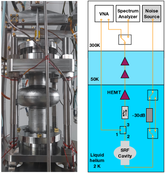
Figure 1: Left: the single-cell SRF cavity equipped with frequency tuner. Right: Schematic of the microwave electronics for DPDM searches. The VNA measures the net amplification factor $\displaystyle G_{\rm net}$ of the amplifier circuit consisting of an isolator, a HEMT amplifier and two room-temperature amplifiers. The noise source and the spectrum analyzer calibrate the resonant frequencies $\displaystyle f_{0}^{i}$. The time-domain signals from the SRF, with sequential amplification, are finally recorded by the spectrum analyzer.

III Experimental Operation

Before carrying out DPDM searches, it is essential to calibrate the relevant cavity and amplifier parameters. All calibrated parameters and the corresponding uncertainties are presented in Table. 1. Both the volume of the cavity and the form factor of the TM₀₁₀ mode are determined by numerical modeling software COMSOL, with $\displaystyle<1\%$ uncertainty for $\displaystyle V_{\rm eff}\equiv V\,C/3$.

We present the experimental setup in which the microwave electronics are depicted in the right panel of Fig. 1. The cavity is positioned within a liquid helium environment at a temperature $\displaystyle T\simeq 2$ K and is connected to axial pin couplers. The amplifier circuit consists of an isolator, which serves to prevent the injection of amplifier noise into the cavity, a high-electron mobility transistor (HEMT) amplifier (LNF-LNC0.2_3A), and two room-temperature amplifiers (ZX60-P103LN+). Initially, we used the vector network analyzer (VNA) to measure the net amplification factor $\displaystyle G_{\rm net}$ of the amplifier circuit, which considers the sequential amplification and potential decays within the line. Next, we conducted decay measurements with a noise source that went through the cavity, the amplifier line, and the spectrum analyzer, to calibrate the cavity loaded quality factor, $\displaystyle Q_{L}\equiv Q_{0}/(\beta+1)$. The cavity coupling factor $\displaystyle\beta$, was calibrated in combination with the results of the standard vertical test stand.

For each scan step, we used the noise source to calibrate the resonant frequency $\displaystyle f_{0}$ of the cavity by locating the peak of the power spectral density (PSD). Immediately after, we switched off the noise source and applied the $\displaystyle 30$ dB attenuator to prevent the external noise from entering the cavity. We then used the spectrum analyzer to record the time-domain signals from the SRF cavity and amplifiers. Each scan took $\displaystyle t_{\rm int}=100$ seconds. After each scan, the value of $\displaystyle f_{0}$ was adjusted by approximately $\displaystyle 1.3$ kHz and the calibration of $\displaystyle f_{0}$ was restarted. A total of $\displaystyle N_{\rm bin}=1150$ scans were conducted, covering a frequency range of approximately $\displaystyle 1.37$ MHz. The highest resonant frequency, denoted by $\displaystyle f_{0}^{\rm max}$, occurred when the frequency tuner was not applied. The calibration process for $\displaystyle G_{\rm net}$, $\displaystyle Q_{L}$, and $\displaystyle\beta$ was conducted multiple times during the whole scan process, with uncertainties given by the measurement deviation.

One key challenge of DPDM searches using SRF is to ensure any potential signal induced from DPDM is within the resonant bin, as $\displaystyle f_{0}$ may drift with time or oscillate due to microphnics effect Pischalnikov et al. (2019); Romanenko et al. (2023). To determine the stability range of $\displaystyle f_{0}$, denoted as $\displaystyle\Delta f_{0}$, we measured the drift of $\displaystyle f_{0}$ every $\displaystyle 50$ scans, matching the integration time $\displaystyle t_{\rm int}$ of a single scan step, and also assessed the effect of microphonics over the same duration (see Supplemental Material). The microphonics effect produces a resonant frequency distribution with a root mean square of $\displaystyle\delta f_{m}^{\rm rms}=4.1$ Hz, which is dominant over the drift with a maximum deviation of $\displaystyle 1.5$ Hz. To account for any potential deviations in $\displaystyle f_{0}$, we conservatively selected $\displaystyle\Delta f_{0}$ to be $\displaystyle 2.8\,\delta f_{m}^{\rm rms}\simeq 11.5$ Hz, taking into consideration an efficiency of $\displaystyle\eta_{\rm bin}=84\%$ for the recorded signal to optimize the SNR.

	Value	Fractional Uncertainty
$\displaystyle V_{\rm eff}\equiv V\,C/3$	$\displaystyle 693$ mL	$\displaystyle<1\%$
$\displaystyle\beta$	$\displaystyle 0.634\pm 0.014$	$\displaystyle 1.4\%$
$\displaystyle G_{\rm net}$	$\displaystyle(57.30\pm 0.14)$ dB	$\displaystyle 3.1\%$
$\displaystyle Q_{L}$	$\displaystyle(9.092\pm 0.081)\times 10^{9}$	$\displaystyle/$
$\displaystyle f_{0}^{\rm max}$	$\displaystyle 1.2991643795$ GHz	$\displaystyle/$
$\displaystyle\Delta f_{0}$	$\displaystyle 11.5$ Hz	$\displaystyle/$
$\displaystyle t_{\text{int}}$	$\displaystyle 100$ s	$\displaystyle/$

Table 1: Calibrated parameters for SRF cavities and amplifiers used are shown, including their mean values, uncertainties and fractional uncertainties on DPDM-induced power, $\displaystyle F_{j}$.

IV Data Analysis and Constraints

For each scan labelled $\displaystyle i=1,\cdots,N_{\rm bin}$, we focused on the frequency bin centered at $\displaystyle f_{0}^{i}$ with a bandwidth of $\displaystyle\Delta f_{0}$. During each scan, we obtained $\displaystyle N=t_{\rm int}\Delta f_{0}$ samples at the resonant bin, and calculated the average value $\displaystyle\bar{P}_{f_{0}^{i}}$ and standard deviation $\displaystyle\sigma_{f_{0}^{i}}$. We tested the Gaussian noise property by checking that $\displaystyle\sigma_{f_{0}^{i}}\simeq\bar{P}_{f_{0}^{i}}$ at each step.

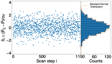
Figure 2: The blue dots show the normalized power excess $\displaystyle\delta_{i}\equiv(\bar{P}_{f_{0}^{i}}-\bar{P})/\sigma_{\bar{P}}$ at each scan step $\displaystyle i$. Its distribution is shown on the right panel, which can be well fit by a standard normal distribution.

The values of $\displaystyle\bar{P}_{f_{0}^{i}}$ for different $\displaystyle f_{0}^{i}$ indicate the total noise in each resonant bin. The amplifier noise, $\displaystyle P_{\rm amp}$, is almost constant over the entire frequency range examined. Additionally, the subdominant thermal noise in Eq. (2) was linearly proportional to $\displaystyle f_{0}^{i}$, with a variation much smaller than $\displaystyle\sigma_{f_{0}^{i}}$. Thus, we expected the noise in the resonant bins to be independent of $\displaystyle f_{0}^{i}$. To mitigate the potential effects of environmental variation, such as helium pressure fluctuations and mechanical vibrations, we have aggregated every $\displaystyle 50$ contiguous bins to ensure environmental stability within each group. For each group, we performed a constant fit to $\displaystyle\bar{P}_{f_{0}^{i}}$ for different $\displaystyle f_{0}^{i}$, i.e., $\displaystyle\bar{P}\equiv(\Sigma_{i}\bar{P}_{f_{0}^{i}}/{\sigma_{f_{0}^{i}}^{2}})/({\Sigma_{i}1/{\sigma_{f_{0}^{i}}^{2}}})$. We then define the normalized power excess $\displaystyle\delta_{i}\equiv(\bar{P}_{f_{0}^{i}}-\bar{P})/\sigma_{\bar{P}}$, where $\displaystyle\sigma_{\bar{P}}$ is the sample standard deviation of $\displaystyle\bar{P}_{f_{0}^{i}}$ subtracting $\displaystyle\bar{P}$, and presented them in Fig. 2. The right panel of the figure shows a comparison between the counts of normalized power excess and the standard normal distribution to confirm its Gaussianity. Notice that there is no $\displaystyle 3\,\sigma$ deviation in all the bins.

Compared to the analysis strategies employed by traditional haloscopes with $\displaystyle Q_{0}\ll Q_{\rm DM}$, our resonant bins cover only a fraction of the entire frequency band, $\displaystyle\Delta f_{0}Q_{\rm DM}/f_{0}^{i}$. However, we can still test the DPDM with masses within this range and thereby maximize the scan rate. Additionally, the fitting function employed in our study yields a signal power that is attenuated by a factor of $\displaystyle 98\%$. The attenuation effect is less suppressed when compared to low $\displaystyle Q_{0}$ experiments, where higher-order fitting functions are utilized to account for the frequency-dependent cavity response during each scan.

Figure 3: The $\displaystyle 90\%$ exclusion on the kinetic mixing coefficient $\displaystyle\epsilon$ of DPDM based on SRF scan searches performed in this study. Other constraints including FAST radio telescope An et al. (2022), distortion of cosmic microwave background Arias et al. (2012), and SQMS prototype Cervantes et al. (2022a) are shown for comparison.

In addition to the uncertainty $\displaystyle\sigma_{\bar{P}}$ characterizing $\displaystyle\bar{P}$, there are uncertainties in calibrated parameters that may contribute to a biased estimate for DPDM-induced signals. To account for these variances, we introduce dimensionless signals $\displaystyle p_{i}$ normalized by a reference signal power $\displaystyle P_{\rm ref}^{i}\equiv\eta_{\rm bin}\eta_{\rm fit}G_{\rm net}P_{\text{sig}}(m_{A^{\prime}},f_{0}^{i},\epsilon=1)$, along with the corresponding statistical uncertainties

$$p_{i}\equiv\frac{\bar{P}_{f_{0}^{i}}-\bar{P}}{P_{\rm ref}^{i}},\quad\sigma_{p_{i}}^{2}=\left(\frac{\sigma_{\bar{P}}}{P_{\rm ref}^{i}}\right)^{2}\left(1+\delta_{i}^{2}\sum_{j}F_{j}^{2}\right),$$ (5)

where $\displaystyle F_{j}$ represents the translation of uncertainties for parameters $\displaystyle j\in\{V_{\rm eff},\beta,G_{\rm net}\}$ into variations of $\displaystyle P_{\rm ref}^{i}$, as listed in Table. 1 and derived in Supplemental Materials. The probability function is then the product of different bins $\displaystyle i$ given by

$$\displaystyle{\rm Pr}\left(p_{i}|\epsilon,m_{A^{\prime}}\right)=\prod_{i}\frac{1}{\sqrt{2\pi}\sigma_{p_{i}}}\exp\left(-\frac{(p_{i}-\epsilon^{2})^{2}}{2\sigma_{p_{i}}^{2}}\right)/{\rm Const},$$ (6)

where $\displaystyle{\rm Const}$ is the normalization factor irrelevant in the calculation. In practice, due to the narrow bandwidth $\displaystyle\Delta f_{0}$ compared with DPDM width $\displaystyle\approx m_{A^{\prime}}/(2\pi Q_{\rm DM})$, the products in Eq. (6) only consider the two nearby bins. From Eq. (6) we can set the $\displaystyle 90\%$ upper limit on the kinetic mixing coefficient $\displaystyle\epsilon$ for a given DPDM mass $\displaystyle m_{A^{\prime}}$. The results are shown in Fig. 3. The high quality factor of SRF significantly boosts sensitivity, leading to the most stringent constraints compared to other limitations across a wide range of investigated masses. The reached sensitivity is well-estimated by Eq. (4).

V Discussion

In this study, we utilized a tunable single-cell $\displaystyle 1.3$ GHz elliptical cavity to search for DPDM. Our findings establish the most stringent exclusion limit across a majority of the scanned mass window, achieving a depth of sensitivity of up to $\displaystyle\epsilon\sim 2.2\times 10^{-16}$. This result demonstrates that employing cavities with high-quality factors significantly enhances the sensitivity towards the kinetic mixing coefficient of DPDM. Our experiment presents the first scan results using a tunable SRF cavity, which covers a frequency range of $\displaystyle 1.37$ MHz within DPDM’s mass window. The scanning process started from an initial resonant frequency of $\displaystyle f_{0}^{\rm max}\simeq 1.299$ GHz. We are currently designing a tuning apparatus to extend the scan window, and we will report corresponding experimental results in future work.

The significantly high quality factors of SRF cavities enable various further upgrades to enhance their sensitivity. For example, coupling a single cavity mode to a multi-mode resonant systems with non-degenerate parametric interactions Li et al. (2020); Chen et al. (2022a); Wurtz et al. (2021); Jiang et al. (2023b); Chen et al. (pear) can broaden the effective bandwidth of each scan without losing sensitivity within it. One can also exploit squeezing technology Zheng et al. (2016); Malnou et al. (2019); Backes et al. (2021); Lehnert (2021); Jewell et al. (2023) or non-demolition photon counting Dixit et al. (2021); Agrawal et al. (2023) to go beyond the standard quantum limit. A network of DPDM detectors simultaneously measuring at the same frequency band will not only increase the sensitivity Chen et al. (2022a); Brady et al. (2022), but also reveal macroscopic properties and the microscopic nature of the DPDM sources, such as the angular distribution and polarization Foster et al. (2021); Chen et al. (2022b).

Supplemental Materials: SRF Cavity Searches for Dark Photon Dark Matter: First Scan Results

Appendix A Resonant Frequency Calibration and Stability

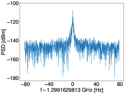
Figure S1: An example of PSD injected by a noise source to calibrate the resonant frequency by finding the peak with an integration time of $\displaystyle 10$ seconds.

Calibration of the resonant frequency is essential in the search for DPDM using SRF cavities, due to their high quality factor and narrow bandwidth. We accomplished this by injecting a broadband noise source into the cavity and recording the signal with a spectrum analyzer for $\displaystyle 10$ seconds. We then selected the frequency bin with the peak power spectral density (PSD) as the resonant frequency. An example of the PSD is presented in Fig. S1. Following each calibration, we switched off the noise source and waited for the excited field to decay until the cavity was dominated by noise. Each data recording began immediately thereafter.

The stability analysis included both frequency drift and microphonics effect. For every group of $\displaystyle 50$ scan steps, we tested the drift of the resonant frequency for $\displaystyle 100$ seconds, which is equivalent to the data recording time for one scan. The drift of $\displaystyle f_{0}$, denoted by $\displaystyle\delta f_{d}$, is presented in the left panel of Fig. S2. As we selected the peak of the PSD as the resonant frequency bin every $\displaystyle 10$ seconds, the $\displaystyle 100$-second interval included the $\displaystyle 10$-step evolution of $\displaystyle\delta f_{d}$. In most cases, we observed a gradual increase over time due to the resistance of the cavity to mechanical deformation. The maximal value of the frequency drift, $\displaystyle\delta f_{d}^{\rm max}$, is $\displaystyle 1.5$ Hz.

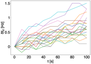
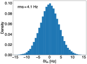
Figure S2: Left: measurements of resonant frequency drift for a duration of $\displaystyle 100$ seconds. Every colored line represents a test that was conducted every $\displaystyle 50$ scan steps. Right: histogram of resonant frequency’s oscillatory deviation.

On the other hand, the microphonics effect that leads to oscillatory deviation of the resonant frequency Pischalnikov et al. (2019) does not necessarily reflect on the peak position of PSDs with $\displaystyle 10$-second intervals. Instead, we employed the Digital Phase-Locked Loops (PLL) system available in the Vertical Test Facility (VTS) to evaluate the microphonics Pischalnikov et al. (2019). This system introduces a coherent field into the SRF cavity, and the oscillatory deviation of the resonant frequency is reflected in the change rate of the relative phase, given by $\displaystyle 2\pi\,\delta f_{m}=\mathrm{d}\phi/\mathrm{d}t$. In the right panel of Fig. S2, we present the results of the microphonics test for a $\displaystyle 100$-second interval. The histogram of $\displaystyle\delta f_{m}$ indicates the dominance of the drift effect, which follows a Gaussian distribution with a root mean square (rms) value of $\displaystyle\delta f_{m}^{\rm rms}=4.1$ Hz. The DPDM signals are expected to broaden according to the same Gaussian distribution, with an efficiency $\displaystyle\eta_{\rm bin}$ given by $\displaystyle\eta_{\rm bin}=\text{erf}\left(\Delta f_{0}/(2\sqrt{2}\delta f_{m}^{\rm rms})\right)$, where $\displaystyle\text{erf}(x)$ represents the error function. By maximizing the signal-to-noise ratio (SNR) $\displaystyle\propto\eta_{\rm bin}/\sqrt{\Delta f_{0}}$, the choice of $\displaystyle\Delta f_{0}$ can be optimized, which results in $\displaystyle\Delta f_{0}\simeq 2.8\,\delta f_{m}^{\rm rms}\simeq 11.5$ Hz and $\displaystyle\eta_{\rm bin}\simeq 84\%$.

Appendix B Data Characterization

This section presents the recorded data obtained during the scan searches. Only the bin at the resonant frequency is taken into account in the data analysis for each scan. Each bin consists of $\displaystyle N=t_{\rm int}\Delta f_{0}=1150$ samples of measured power, corresponding to the integration time $\displaystyle t_{\rm int}=100$ s with the bin size $\displaystyle\Delta f_{0}=11.5$ Hz. In a power-law detection, the observable is two-point correlation function in terms of voltage. The Gaussian nature of the voltage fluctuation thus leads to a chi-squared distribution with $\displaystyle 2$ degrees of freedom of the measured power, satisfying $\displaystyle\bar{P}_{f_{0}^{i}}\approx\sigma_{f_{0}^{i}}$. We show values of $\displaystyle\bar{P}_{f_{0}^{i}}/\sigma_{f_{0}^{i}}$ for different scan step $\displaystyle i$ in the left panel of Fig. S3. Their distribution is indeed centered on $\displaystyle 1$, and follows a Gaussian distribution due to the central limit theorem.

We translate the power into the corresponding effective temperature $\displaystyle T_{\rm eff}^{i}$ of each scan through $\displaystyle T^{i}_{\rm eff}\equiv{\bar{P}_{f_{0}^{i}}}/{(G_{\rm net}k_{b}\,\Delta f_{0})}$. The right panel of Fig. S3 shows their distribution, ranging from $\displaystyle 2.6$ K to $\displaystyle 3.4$ K, with a mean of $\displaystyle 3.0$ K. The variation is suppressed by a factor of $\displaystyle\sqrt{N}\approx 34$ compared to typical values of $\displaystyle\sigma_{f_{0}^{i}}$. Although there is a slight upward trend in the distribution due to environmental effects such as helium pressure fluctuations, the deviation is not significant. We addressed this effect by grouping every $\displaystyle 50$ adjacent bins and testing for deviations from a constant fit. The histogram of normalized power excess in Fig. 2 is well-modeled by a Gaussian distribution with no observed deviations greater than $\displaystyle 3\,\sigma$.

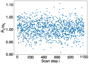
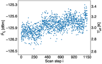
Figure S3: Left: The values of $\displaystyle\bar{P}_{f_{0}^{i}}/\sigma_{f_{0}^{i}}$ for each scan. Right: The power $\displaystyle\bar{P}_{f_{0}^{i}}$ and the corresponding effective temperature $\displaystyle T^{i}_{\rm eff}$ for each scan.

The application of constant fit and normalized excess introduces an attenuation factor $\displaystyle\eta_{\rm fit}$ to a potential signal. In our case, there are $\displaystyle 50$ resonant bins in a group, so any signal entering the fit function $\displaystyle\bar{P}$ will be reduced by a factor of $\displaystyle 1/50$, thereby resulting in $\displaystyle\eta_{\rm fit}=98\%$. Note that increasing the number of bins in a group can decrease the influence of the attenuation factor. Moreover, the sample standard deviation of $\displaystyle\bar{P}_{f_{0}^{i}}$ minus $\displaystyle\bar{P}$, denoted as $\displaystyle\sigma_{\bar{P}}$, can be increased by a potential signal. However, we conservatively neglect this influence in our analysis.

Appendix C Fractional Uncertainties from Calibrated Parameters

For a physical quantity $\displaystyle\mathcal{N}(x_{1},x_{2}...)$ that is a function of measured observables $\displaystyle x_{1},x_{2}\cdots x_{j}$, its uncertainty is calculated through error propagation formula:

$$\displaystyle\sigma_{\mathcal{N}}^{2}=\sum_{j}\left(\frac{\partial\mathcal{N}}{\partial x_{j}}\right)^{2}\sigma_{x_{j}}^{2}.$$ (S1)

In the maintext, we introduced the dimensionless signals $\displaystyle p_{i}\equiv(\bar{P}_{f_{0}^{i}}-\bar{P})/P_{\rm ref}^{i}$, whose variance can be calculated using Eq. (S1),

$$\sigma_{p_{i}}^{2}= \left(\frac{\partial p_{i}}{\partial\bar{P}_{f_{0}^{i}}}\sigma_{\bar{P}}\right)^{2}+\sum_{j}\left(\frac{\partial p_{i}}{\partial P_{\rm ref}^{i}}\frac{\partial P_{\rm ref}^{i}}{\partial j}\sigma_{j}\right)^{2}$$ (S2)

$$= \left(\frac{\sigma_{\bar{P}}}{P_{\rm ref}^{i}}\right)^{2}\left(1+\delta_{i}^{2}\sum_{j}F_{j}^{2}\right).$$

Here the sum of calibrated parameters include $\displaystyle j\in\{V_{\rm eff},\beta,G_{\rm net}\}$, and the fractional uncertainties $\displaystyle F_{j}$ are defined as

$$\sum_{j}F_{j}^{2}\equiv\sum_{j}\left(\frac{\partial P_{\rm ref}^{i}}{\partial j}\frac{\sigma_{j}}{P_{\rm ref}^{i}}\right)^{2}=\frac{\sigma_{V_{\rm eff}}^{2}}{V_{\rm eff}^{2}}+\left(\frac{1}{\beta}-\frac{1}{1+\beta}\right)^{2}\sigma_{\beta}^{2}+\frac{\sigma_{G_{\text{net}}}^{2}}{G_{\text{net}}^{2}}.$$ (S3)

Notice that in this calculation, we take $\displaystyle G_{\text{net}}$ as the dimensionless amplification factor, i.e., $\displaystyle(56.52\pm 0.08)$ dB$\displaystyle\rightarrow 10^{(5.652\pm 0.008)}$.

Appendix D Calibration of $\displaystyle Q_{L}$ and $\displaystyle\beta$

The rate at which cavity mode decays is proportional to the inverse of its quality factor. The loaded quality factor, $\displaystyle Q_{L}$, which quantifies the inverse of the total energy loss rate, is determined by contributions from both intrinsic loss and energy extraction, as given by

$$\displaystyle\frac{1}{Q_{L}}=\frac{1}{Q_{0}}+\frac{1}{Q_{\rm ext}},$$ (S4)

where $\displaystyle Q_{0}$ and $\displaystyle Q_{\rm ext}$ represent the intrinsic and external quality factors, respectively. As $\displaystyle Q_{L}$ is dependent on the field strength within the cavity Romanenko and Schuster (2017), it was calibrated using a noise source that excited low field strength, thereby enabling it to converge to a value where only thermal noise exists in the cavity. Specifically, after turning off the noise source, the excited field decayed exponentially, i.e.,

$$\displaystyle P(t)=P(t_{0})e^{-(t-t_{0})/\tau}$$ (S5)

where $\displaystyle\tau$ represents the decay time. To determine the quality factor ($\displaystyle Q_{L}$) of the decay, the value of $\displaystyle\tau$ was fitted to yield $\displaystyle Q_{L}=2\pi f_{0}\tau$.

The cavity coupling factor $\displaystyle\beta$ is defined as the ratio between the energy delivered to the readout antenna and the internal dissipation, i.e.,

$$\beta=\frac{Q_{L}}{Q_{\rm ext}-Q_{L}}.$$ (S6)

Therefore, the measurement of $\displaystyle Q_{\rm ext}$, whose value is independent of the field strength inside the cavity, can be used to determine $\displaystyle\beta$. This measurement can be carried out using the standard vertical test stand Melnychuk et al. (2014) involving both the measurement of forward and reflected power and decay measurement.

Appendix E Dark Photon Dark Matter and Cavity Response

In this section, we review the profile of dark photon dark matter (DPDM) used in the maintext, and presents how a cavity mode is excited by DPDM or thermal noise. The standard halo model assumes that dark matter has undergone the process of virialization, which balances the gravitational potential energy of the system with the kinetic energy of its components. In the laboratory frame, the local dark matter velocity distribution satisfies

$$\mathcal{F}(\vec{v}\,)=\left(2\pi v_{\text{vir}}^{2}/3\right)^{-3/2}\,\exp\left(-\frac{3(\vec{v}-\vec{v}_{g})^{2}}{2v_{\text{vir}}^{2}}\right),$$ (S7)

where $\displaystyle v_{\text{vir}}\approx 9\times 10^{-4}c$ is the virial velocity in terms of the speed of light, and $\displaystyle|\vec{v}_{g}|\approx(2/3)^{1/2}v_{\text{vir}}$ is the Earth velocity in the galactic frame Turner (1990); Lacroix et al. (2020).

Bosonic dark matter with a mass below $\displaystyle\mathcal{O}(1)$ eV exhibits wave-like properties due to their high occupation number. The frequency of non-relativistic wave-like dark matter is $\displaystyle 2\pi f\approx m_{\rm DM}(1+v^{2}/2)$. The distribution of this frequency comes from Eq. (S7) and can be well approximated by Brubaker et al. (2017); Cervantes et al. (2022b)

$$\mathcal{F}_{\rm DM}(f)=2\left(\frac{f-f_{\rm DM}}{\pi}\right)^{1/2}\left(\frac{3}{1.7f_{\rm DM}v_{\text{vir}}^{2}}\right)^{3/2}\exp\left(-\frac{3(f-f_{\rm DM})}{1.7f_{\rm DM}v_{\text{vir}}^{2}}\right),$$ (S8)

where $\displaystyle 2\pi f_{\rm DM}\equiv m_{\rm DM}$ corresponds to the frequency of rest mass $\displaystyle m_{\rm DM}$. Eq. (S8) satisfies the normalization condition $\displaystyle\int\mathcal{F}_{\rm DM}(f)\,\mathrm{d}f=1$.

For DPDM searches in this study, the signal power spectral density (PSD) in Eq. (1) of the maintext depends on the two-point correlation function of DPDM wavefunctions. Under the Lorenz gauge condition $\displaystyle\partial_{\mu}A^{\prime\mu}=0$, we can determine the DPDM correlation from both the local energy density of dark matter, i.e., $\displaystyle\langle\partial_{t}\vec{A}^{\prime}\cdot\partial_{t}\vec{A}^{\prime*}\rangle=\rho_{\rm DM}$ and the energy distribution in Eq. (S8), yielding:

$$\langle\vec{A}^{\prime}(f)\cdot\vec{A}^{\prime*}(f^{\prime})\rangle=\rho_{\rm DM}\,\mathcal{F}_{\rm DM}\left(f\right)\delta\left(f-f^{\prime}\right)/\left(4\pi^{2}\bar{f}f\right),$$ (S9)

where $\displaystyle\bar{f}\equiv\int f\mathcal{F}_{\rm DM}(f)\mathrm{d}f\approx m_{A^{\prime}}/(2\pi)$ is the average frequency. Here $\displaystyle\langle\cdots\rangle$ denotes the ensemble average of DPDM fields. These fields can be described as an incoherent superposition of individual vector fields Guo et al. (2019); Chen et al. (2022b). The directions of the DPDM fields are thus isotropically distributed, resulting in a factor of $\displaystyle 1/3$ for the correlation between DPDM fields along a given axis, compared to Eq. (S9).

We next consider the Maxwell equation coupled with the effective current induced by DPDM, i.e., $\displaystyle\vec{J}_{\text{eff}}=\epsilon\,m_{A^{\prime}}^{2}\vec{A}^{\prime}$,

$$\Box\vec{E}(t,\vec{x})=\epsilon\,m_{A^{\prime}}^{2}\,\partial_{t}\vec{A^{\prime}}(t,\vec{x}).$$ (S10)

The boundary condition of a cavity decomposes the electric field into a discrete sum of orthogonal cavity modes

$$\vec{E}(t,\vec{x})=\sum_{n}e_{n}(t)\vec{E}_{n}(\vec{x}),$$ (S11)

where $\displaystyle e_{n}(t)$ parameterize time-evolution of each mode. $\displaystyle\vec{E}_{n}(\vec{x})$ form a complete and orthogonal basis within the cavity

$$\nabla^{2}\vec{E}_{n}+(2\pi f_{n})^{2}\vec{E}_{n}=0,\qquad\int\mathrm{d}V\vec{E}_{n}\cdot\vec{E}_{m}^{*}=\delta_{mn}$$ (S12)

with resonant frequency labelled by $\displaystyle f_{n}$.

One can take Eq. (S11) into Eq. (S10), and project it with the ground mode $\displaystyle\vec{E}_{0}$ that has the largest overlapping with DPDM. The equation of motion in the frequency domain becomes

$$\left(f^{2}-f_{0}^{2}-\mathrm{i}\frac{ff_{0}}{Q_{L}}\right)e_{0}(f)=\frac{\mathrm{i}\,\epsilon\,m_{A^{\prime}}^{2}\,f}{2\pi}\int\vec{E}_{0}\cdot\vec{A^{\prime}}(f)\,\mathrm{d}V+\sqrt{\frac{2f_{0}}{Q_{0}}}\,f\,{u}_{0}(f),$$ (S13)

where we take into account the cavity energy loss and dissipation due to intrinsic loss, characterized by the load quality factor $\displaystyle Q_{L}$ and intrinsic quality factor $\displaystyle Q_{0}$, respectively. The last term in Eq. (S13) is the contribution of thermal noise $\displaystyle u_{0}(f)$, which arises due to the fluctuation-dissipation theorem. The two-point correlation function of thermal noise is

$$\langle u_{0}(f)u_{0}^{*}(f^{\prime})\rangle=f\,n_{\rm occ}\,\delta(f-f^{\prime}),$$ (S14)

where $\displaystyle n_{\rm occ}\approx k_{b}T/(hf)$ is the thermal occupation number, and $\displaystyle h$ is the Planck constant.

The energy stored in the cavity mode, i.e., $\displaystyle U_{0}\equiv\iint\mathrm{d}f\mathrm{d}f^{\prime}\langle e_{0}(f)e_{0}(f^{\prime})\rangle$ come directly from Eq. (S13), which contains both the signal and thermal noise $\displaystyle U_{0}=U_{\rm sig}+U_{\rm th}$. The signal part is

$$U_{\rm sig} =\epsilon^{2}m^{3}_{A^{\prime}}\iint\frac{\mathrm{d}f\mathrm{d}f^{\prime}}{8\pi^{3}}\frac{f\,\rho_{\rm DM}\,\mathcal{F}_{\rm DM}\left(f\right)\,\delta(f-f^{\prime})}{(f^{2}-f_{0}^{2})^{2}+\left(ff_{0}/Q_{L}\right)^{2}}\,V\,\frac{C}{3}$$ (S15)

$$\approx\frac{Q_{L}}{8\pi f_{0}}\epsilon^{2}m_{A^{\prime}}^{2}\,V\,\frac{C}{3}\,\rho_{\rm DM}\,\mathcal{F}_{\rm DM}(f_{0}),$$

where we assume that the cavity response width $\displaystyle f_{0}/Q_{L}$ is much narrower than the DPDM width of $\displaystyle f_{A^{\prime}}/10^{6}$ to simplify the expression. The DPDM correlation in Eq. (S9) is used, rendering the form factor

$$C \equiv\frac{3}{V}\langle\left|{\int}_{V}\,\vec{E}_{0}\cdot\hat{A^{\prime}}\,\mathrm{d}V\right|^{2}\rangle$$ (S16)

$$=\frac{3}{V}\int\frac{\mathrm{d}^{2}\Omega}{4\pi}\left|\int\mathrm{d}V\vec{E}_{0}\cdot\hat{\Omega}\right|^{2}$$

$$=\frac{1}{V}\left|{\int}_{V}\,\vec{E}_{0}\,\mathrm{d}V\right|^{2}$$

for randomized DPDM. In Fig. S4, we show the electric field distribution of the TM₀₁₀ mode of the single-cell SRF cavity used in this study, which gives a form factor $\displaystyle C\approx 0.53$.

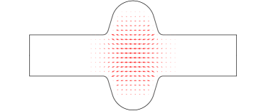
Figure S4: Single-cell SRF cavity with ground mode TM₀₁₀ at $\displaystyle 1.3$ GHz. The electric field lines are shown in red, whose length is proportional to the electric field strength.

The signal power is read from an antenna from the cavity, which takes the form

$$P_{\text{sig}}=\frac{\beta}{\beta+1}\,\frac{2\pi f_{0}}{Q_{L}}\,U_{\rm sig}=\frac{1}{4}\epsilon^{2}\,\frac{\beta}{\beta+1}\,V\,\frac{C}{3}\,m_{A^{\prime}}^{2}\,\rho_{\rm DM}\,\mathcal{F}_{\rm DM}(f_{0}),$$ (S17)

where $\displaystyle\beta/(\beta+1)$ is the fraction of energy delivered into the antenna in terms of the total energy loss of the cavity.

Similarly, the power of thermal noise is

$$P_{\rm th}=\frac{\beta}{\beta+1}\frac{2\pi f_{0}}{Q_{L}}\frac{2f_{0}}{Q_{0}}\int\mathrm{d}f\mathrm{d}f^{\prime}\frac{ff^{\prime}\,\langle u_{0}(f)u_{0}^{*}(f^{\prime})\rangle}{(f^{2}-f_{0}^{2})^{2}+\left(ff_{0}/Q_{L}\right)^{2}}=2\pi\,\frac{\beta}{\beta+1}\,k_{b}T\frac{f_{0}}{Q_{0}}.$$ (S18)