Impact of radiative cooling on the magnetised geometrically thin accretion disk around Kerr black hole

Abstract

It is believed that the spectral state transitions of the outbursts in X-ray binaries (XRBs) are triggered by the rise of the mass accretion rate due to underlying disc instabilities. Recent observations found that characteristics of disc winds are probably connected with the different spectral states, but the theoretical underpinnings of it are highly ambiguous. To understand the correlation between disc winds and the dynamics of the accretion flow, we have performed General Relativistic Magneto-hydrodynamic (GRMHD) simulations of an axisymmetric thin accretion disc with different accretion rates and magnetic field strengths. Our simulations have shown that the dynamics and the temperature properties depend on both accretion rates and magnetic field strengths. We later found that these properties greatly influence spectral properties. We calculated the average coronal temperature for different simulation models, which is correlated with high-energy Compton emission. Our simulation models reveal that the average coronal temperature is anti-correlated with the accretion rates, which is correlated with the magnetic field strengths. We also found that the structured component of the disc winds (Blandford-Payne disc wind) predominates as the accretion rates and magnetic field strengths increase. In contrast, the turbulent component of the disc winds ($B_{\rm tor}$ disc wind) predominates as the accretion rates and magnetic field strengths decrease. Our results suggest that the disc winds during an outburst in XRBs can only be understood if the magnetic field contribution varies over time (e.g., MAXI J1820+070).

1 Introduction

Black hole X-ray binaries (BH-XRBs) are one of the most observed and studied astrophysical sources in the literature. They are primarily observed during their outbursts. In an outburst, the source undergoes a cycle of processes known as the ‘Q’ diagram (Belloni et al., 2011; Belloni & Motta, 2016; Ingram & Motta, 2019). Understanding different parts of the ‘Q’ diagram (hard, intermediate, and soft states) is becoming less and less ambiguous with time, although the transitions between different parts still need to be explored in great detail.

An outburst can be classified into two phases, i.e., the rising and decaying phases. A hard state is observed in both phases. Common consensuses are that the accretion rate alone triggers the spectral state transitions in X-ray binaries (see e.g., Narayan et al., 1998; Yuan & Narayan, 2014, for review). Very recent observations try to couple outflows/wind with the different spectral states of X-ray binaries (e.g., Gallo et al., 2005; Miller et al., 2006; Ponti et al., 2012; Neilsen, 2013; Díaz Trigo & Boirin, 2016; Tetarenko et al., 2018). In the black hole X-ray binaries MAXI J1820+070 and MAXI J1803-298, many observations reported clear signatures of disc-wind in both the hard states in its 2018 outburst (Muñoz-Darias et al., 2019; Mata Sánchez et al., 2022). However, the rising hard state of MAXI J1820+070 shows a higher degree of optical polarisation than the decaying hard state, which is found in an intrinsically unpolarised state (Kosenkov et al., 2020). Possibly, the rising phase is dominated by Blandford-Payne mechanism driven disc-wind (BP disc-wind, structured magnetic field)(Blandford & Payne, 1982), whereas, in the decaying phase, turbulent toroidal magnetic field driven disc-wind or thermal pressure driven disc-wind may dominate (unstructured magnetic field). Keeping all of these in mind, it’s possible that XRBs disc winds are the missing piece to the puzzle for figuring out how the spectral state transition happens during an outburst. These facts hint that during an outburst, the strength and structure of the magnetic field are expected to change along the timeline. Therefore, in general, both the accretion rate, as well as the magnetic field configuration, may be important for the understanding of an outburst of XRBs.

It is clear from the above discussion that the underlying disc winds and their properties may help infer the triggers for the spectral state transitions in X-ray binaries. Earlier thin-disc general relativistic magnetohydrodynamic (GRMHD) simulations show different components of disc-winds from the accretion disc (Vourellis et al., 2019; Vourellis & Fendt, 2021). Later, Dihingia et al. (2021); Dihingia & Vaidya (2022) found strong signatures of BP dominated disc winds with strong and inclined magnetic field configurations. Dihingia et al. (2022) also suggested that a truncated accretion disc may be suitable for understanding the rising phase of the ‘Q’ diagram. However, in these studies, they do not consider any contribution from the radiative cooling processes, which is very consequential in the context of outbursts. Radiative cooling becomes particularly unavoidable during the outburst’s soft and soft-intermediate states. Recently, Dexter et al. (2021) showed that strongly magnetised accretion flow could produce the luminosity of a hard state with the sub-Eddington accretion rate. In a similar context, Wielgus et al. (2022) have recently demonstrated using radiative GRMHD that the spectra of a geometrically thick disc (puffy disc) resemble the intermediate states between soft and hard emission states of BH-XRBs. In this paper, in order to understand the dynamical and spectral features of the accretion disc, we study thin accretion discs with radiative cooling with different magnetic field strengths and accretion rate limits. Finally, we try correlating them with a different part of the ‘Q’ diagram.

This work follows Dihingia et al. (2023) in terms of GRMHD with radiative cooling, where we consider a two-temperature accretion flow. The electrons in the fluids are subjected to radiative cooling by Bremsstrahlung, synchrotron, synchrotron self-comptonisation, and black body radiation. The electrons heat up due to the Coulomb collision and magnetic heating processes (turbulent and reconnection heating). In the next section (Section 2), we discuss the mathematical details of disc setup, radiative processes, etc. In Sections 3-7, we discuss results obtained from different simulation models and their interpretations and analyses. Finally, in Section 8, we conclude our results with a discussion on the astrophysical implications of our results and future plans.

Note that throughout the manuscript, we solve the equations and express the quantities in geometrised units, where $G=M_{\bullet}=c=1$. $G,M_{\bullet}$ and $c$ refer to the universal gravitational constant, the mass of the black hole, and the speed of light, respectively. In this system of units, mass, length, and time scales are presented in terms of $M_{\bullet},r_{g}=GM_{\bullet}/c^{2}$, and $t_{g}=GM_{\bullet}/c^{3}$, respectively.

2 Model setup

In this section, we discuss the mathematical formalism of this study. We have employed the GRMHD code BHAC with an adaptive-mesh refinement (AMR) scheme to carry out 2D (axisymmetric) simulations of magnetised thin-discs around Kerr black holes. The governing equations of ideal GRMHD in terms of conservation laws are as follows (see Del Zanna et al., 2007; Rezzolla & Zanotti, 2013),

$$\partial_{t}\left(\sqrt{\gamma}\boldsymbol{U}\right)+\partial_{i}\left(\sqrt{\gamma}\boldsymbol{F^{i}}\right)=\sqrt{\gamma}\boldsymbol{S}\,.$$ (1)

In the presence of radiative cooling, the source term is modified as $\boldsymbol{S}=\boldsymbol{S_{0}}+\boldsymbol{S^{\prime}}$, where $\boldsymbol{S^{\prime}}$ is the contribution of all the cooling and heating processes. The explicit form of the additional source term can be written as (Dihingia et al., 2023),

$$\boldsymbol{S^{\prime}}=\begin{pmatrix}0\\ -\alpha\gamma v_{j}\Lambda\\ -\alpha\gamma\Lambda\\ 0\\ \end{pmatrix}\,,$$ (2)

where the symbols $\alpha$, $\gamma$, $v_{j}$, and $\Lambda$ denote, respectively, the lapse function, the Lorentz factor, the covariant fluid three-velocity, and the total radiation-cooling term. The other symbols have their usual meaning in ideal GRMHD, i.e., conserved variables $\boldsymbol{U}$, fluxes $\boldsymbol{F^{i}},$ and sources $\boldsymbol{S_{0}}$. The detailed expression of these variables in the case of ideal GRMHD without radiative cooling has been reported by Porth et al. (2017) [see Eqs. (23) and (30) there (for detail follow Rezzolla & Zanotti, 2013)].

Equation 1 describes the single-fluid MHD equations. To expand our investigation to a two-temperature framework, we additionally solve the electron-entropy equation including dissipative heating, Coulomb interactions, and radiation-cooling processes (e.g., Sądowski et al., 2017), i.e.,

$$T_{e}\nabla_{\mu}\left(\rho u^{\mu}\kappa_{e}\right)=fQ+\Lambda_{\rm ei}-\Lambda\,,$$ (3)

where $\kappa_{e}:=\exp[(\tilde{\Gamma}_{e}-1)s_{e}]$, and subsequently $s_{e}:=p/\rho^{\tilde{\Gamma}_{e}}$ is the electron entropy per particle. Here, $\tilde{\Gamma}_{e}$ represents the adiabatic index for the electrons. $f$ is the fraction of dissipating heating $(Q)$ transferred to the electrons, and $\Lambda_{\rm ei}$ is the rate of energy transferred to the electrons from the ions due to the Coulomb interaction. In order to solve the electron entropy equation (Eq. 3), we assume charge neutrality, i.e., $n=n_{e}=n_{i}$ (equal number densities for electrons and ions), and also assume that the four-velocity of the electrons, ions, and the flow be the same, i.e., $u^{\mu}=u^{\mu}_{e}=u^{\mu}_{i}$. This does not have to be strictly true, but it is a plausible first approximation. For instance, in the solar wind, the relative speeds of different particle species can become close to the Alfven speed (Bourouaine et al., 2013). However, a similar approach has been widely used for two-temperature frameworks in semi-analytical and numerical studies (e.g., Narayan & Yi, 1995; Nakamura et al., 1996; Manmoto et al., 1997; Ressler et al., 2015; Chael et al., 2018; Dihingia et al., 2018; Dihingia et al., 2020). In this work, we follow Ressler et al. (2015) to treat dissipative-heating terms and update the electron’s entropy explicitly following conservation principles. We solve all flow variables using Eqs. (1) and (3) following Dihingia et al. (2023). By obtaining the internal energy of flow and electrons, we calculate the internal energy contribution of protons and subsequently calculate the temperatures of electrons ($T_{e}$) and ions ($T_{i}$). For simplicity, we consider the ideal equation of state with three adiabatic indexes for flow (gas as a whole), electrons, and ions as $\tilde{\Gamma}_{g}=13/9$, $\tilde{\Gamma}_{e}=4/3$, and $\tilde{\Gamma}_{p}=5/3$ (e.g., Shiokawa et al., 2012; Ryan et al., 2017, 2018; Dihingia et al., 2023). These choices are also supported by simulations with variable adiabatic indexes for each component (Sądowski et al., 2017).

2.1 Dissipative and radiative processes

The temperatures and flow variables are calculated by solving Eqs. 1 and 3 can be used to calculate the dissipative-heating fraction, Coulomb interaction rate, and radiation cooling rates. With the exception of the black body cooling process, most of the physical processes present in the accretion flow are identical to those described in our earlier work (Dihingia et al., 2023). Nevertheless, for the sake of completeness, we list them once again here. We apply a turbulent-heating prescription to determine $f$. We employ Howes (2010, 2011) to model this quantity and set up $f$ as

$$f:=\frac{1}{1+Q_{i}/Q_{e}}\,,$$ (4)

where

$$\frac{Q_{i}}{Q_{e}}=c_{1}\frac{c_{2}+\beta^{\alpha}}{c_{2}+\beta^{\alpha}}\sqrt{\frac{m_{p}T_{i}}{m_{e}T_{e}}}\exp(-1/\beta)\,,$$

where $m_{e}$ and $m_{p}$ are electron and proton masses, respectively, while $c_{1}=0.92,c_{2}=1.6/(T_{i}/T_{e}),c_{3}=18+5\log(T_{i}/T_{e})$, $\alpha=2-0.2\log(T_{i}/T_{e})$, and $\beta=p_{\rm gas}/p_{\rm mag}$. Also, for comparison, we incorporate the reconnection heating model to calculate factor $f$ with (Rowan et al., 2017),

$$f=\frac{1}{2}\exp\bigg{[}\frac{-(1-\beta/\beta_{\rm max})}{0.8+\sigma_{h}^{0.5}}\bigg{]}\,,$$

where $\beta_{\rm max}=\sigma_{h}/4$ and $\sigma_{h}=b^{2}/\rho h$ with specific enthalpy $h=1+\tilde{\Gamma}_{g}p_{g}/(\tilde{\Gamma}_{g}-1)$. Subsequently, we express the Coulomb interaction rate $(Q_{\rm ei})$, whose explicit form in CGS units is provided by (Spitzer, 1965; Colpi et al., 1984),

$$Q_{\rm ei}=1.6\times 10^{-13}\frac{k_{\rm B}\sqrt{m_{e}}\ln\Lambda_{0}}{m_{p}}n_{e}n_{i}(T_{i}-T_{e})T_{e}^{-3/2}\,,$$ (5)

where we consider $\ln\Lambda_{0}=20$. In order to determine the Bremsstrahlung cooling rate, we adhere Esin et al. (1996). To be more specific, the free-free Bremsstrahlung-cooling rate for an ionised plasma that is composed of electrons and ions is represented by the equation $Q_{\rm br}=Q_{\rm br}^{\rm ei}+Q_{\rm br}^{\rm ee}$. The exact forms of the individual terms are as follows:

$$\begin{aligned} Q_{\rm br}^{\rm ei}=&1.48\times 10^{-22}n_{i}n_{e}\\ &\times\begin{cases}4\sqrt{\frac{2\Theta_{e}}{\pi^{3}}}\left(1+1.781\Theta_{e}^{1.34}\right)\,,&\text{if }\Theta_{e}<1\\ \frac{9\Theta_{e}}{2\pi}\left(\ln\left(1.123\Theta_{e}+0.48\right)+1.5\right)\,,&\text{otherwise.}\end{cases}\end{aligned}$$ (6)

and

$$\begin{aligned} &Q_{\rm br}^{\rm ee}=\\ &\begin{cases}2.56\times 10^{-22}n_{e}^{2}\Theta_{e}^{3/2}\left(1+1.1\Theta_{e}+\Theta_{e}^{2}-1.25\Theta_{e}^{5/2}\right)\,,&\text{if }\Theta_{e}<1\\ 3.24\times 10^{-22}n_{e}^{2}\Theta_{e}\left(\ln(1.123\Theta_{e})+1.28\right)\,,&\text{otherwise.}\end{cases}\end{aligned}$$ (7)

Here, $\Theta_{e}:=k_{\rm B}T_{e}/m_{e}c^{2}$ is defined for the dimensionless electron temperature.

Due to the presence of a high magnetic field, the accretion flow’s hot electrons radiate via the thermal synchrotron process. We consider the rate of synchrotron emission as follows (Esin et al., 1996):

$$\begin{aligned} Q_{\rm cs}=&\frac{2\pi k_{\rm B}T_{i}\nu_{c}^{3}}{3Hc^{2}}+6.76\times 10^{-28}\frac{n_{e}}{K_{2}(1/\Theta_{e})a_{1}^{1/6}}\\ &\times\bigg{[}\frac{1}{a_{4}^{11/2}}\Gamma\left(\frac{11}{2},a_{4}\nu_{c}^{1/3}\right)+\frac{a_{2}}{a_{4}^{19/4}}\Gamma\left(\frac{19}{4},a_{4}\nu_{c}^{1/3}\right)\\ &+\frac{a_{3}}{a_{4}^{4}}\left(a_{4}^{3}\nu_{c}+3a_{4}^{2}\nu_{c}^{2/3}+6a_{4}\nu_{c}^{1/3}+6\right)\exp(-a_{4}\nu_{c}^{1/3})\bigg{]}\,,\\ \end{aligned}$$ (8)

where $H$ is the local scale height of the accretion disc, we estimate it from the gradient of the electron temperature as $H=T_{e}^{4}/|\nabla T_{e}^{4}|$ following (Fragile & Meier, 2009), and finally, $K_{2}$ is the modified Bessel function of the second kind. In (8), the coefficients $a_{1-4}$ are given by,

$$a_{1}=\frac{2}{3\nu_{0}\Theta_{e}^{2}}\,,\quad a_{2}=\frac{0.4}{a_{1}^{1/4}}\,,\quad a_{3}=\frac{0.5316}{a_{1}^{1/2}}\,,\quad a_{4}=1.8899a_{1}^{1/3}\,,$$ (9)

Moreover, $\Gamma(a,x)$ is the “incomplete Gamma function” define as $\Gamma(a,x):=\int_{x}^{\infty}t^{a-1}e^{-t}~{}dt$. In addition, $\nu_{0}:=eB/(2\pi m_{e}c)$ and $\nu_{c}$ are synchrotron characteristic frequencies, where $e$ and $B$ are electronic charge and magnetic field strength in CGS units, respectively. By equating the emissivities of optically thin and thick volumes, synchrotron frequencies can be computed (Esin et al., 1996; Dihingia et al., 2023). Note that Eq. (8) only works with thermal electrons. To ensure that the highly magnetised region contributes negligibly to thermal synchrotron radiation, we adjust Eq. (8) with a cutoff value for the magnetisation $\sigma$, the ratio between rest-mass and magnetic energy densities: $\sigma=b^{2}/\rho$, i.e., $Q^{\prime}_{\rm cs}=\exp(-(\sigma/\sigma_{\rm cut})^{2})Q_{\rm cs}$ with $\sigma_{\rm cut}=10$. We also take into account the synchrotron radiation’s Comptonisation. In our simplified model, we determine the synchrotron radiation’s Compton-enhancement factor at the local cuff off frequency $(\nu_{c})$. Following this, the total radiation-cooling rate is computed as follows:

$$Q_{\rm thin}^{-}=Q_{\rm br}+\eta(\nu_{c})Q^{\prime}_{\rm cs}\,,$$ (10)

where the Compton enhancement factor $(\eta)$ is expressed as (Narayan & Yi, 1995)

$$\eta(\nu_{c})=1+\frac{P(A-1)}{1-PA}\left(1-\left(\frac{3k_{\rm B}T_{e}}{h\nu_{c}}\right)^{\eta_{1}}\right)\,,$$ (11)

with, $P=1-\exp(-\tau_{\rm es})$, $A=1+4\Theta_{e}+16\Theta_{e}^{2}$, $\eta_{1}=1+\ln P/\ln A$, and $\tau_{\rm es}=2\sigma_{\rm T}n_{e}H$, where $\sigma_{\rm T}$ is the electronic Thomson cross section.

The equation 10 gives the total cooling due to optically thin matter. However, in the thin disc, the optically thick components can not be neglected due to the high optical depth. Therefore, we consider generalised cooling formula suggested by Narayan & Yi (1995) and Esin et al. (1996),

$$Q^{-}_{\rm tot}=\frac{4\sigma_{T}T_{e}^{4}/H}{1.5\tau+\sqrt{3}+\tau_{\rm abs}^{-1}}\,,$$ (12)

where $\tau=\tau_{\rm es}+\tau_{\rm abs}$, and $\tau_{\rm abs}=(HQ_{\rm thin}^{-}/\sigma_{T}T_{e}^{4})$. Finally, we included the Coulomb interaction and radiation-cooling terms in the governing equations in code units as $\Lambda_{\rm ei}=Q_{\rm ei}/U_{\rm c}$ and $\Lambda=Q^{-}/U_{\rm c}$, where $U_{\rm c}=\dot{M}_{\rm cgs}c^{2}/r_{g}^{3}$ and $\dot{M}_{\rm cgs}$ is the mass-accretion rate $(\dot{M})$ in CGS units.

2.2 Initial conditions

For this work, we set up a geometrically thin accretion disc as the initial condition for the simulations following Dihingia et al. (2021); Dihingia & Vaidya (2022), which is based on the standard thin-disc model proposed by Novikov & Thorne (1973). In this setup, the initial density distribution on the poloidal plane in Boyer-Lindquist (BL) coordinates are given by,

$$\rho(r,\theta)=\rho_{e}(r)\exp\left(-\frac{\alpha^{2}z^{2}}{H_{e}^{2}}\right);~{}~{}z=r\cos(\theta)\,.$$ (13)

To maintain the geometrical thin nature of the initial disc, we choose $\alpha=2$ and equilibrium disc-height $(H_{e})$ following Riffert & Herold (1995) and Peitz & Appl (1997). In Eq. (13), $\rho_{e}(r)$ provides the density profile on the equatorial plane, which is given by,

$$\rho_{e}(x)=\left(\frac{\Theta_{0}}{\cal K}\right)^{1/(\tilde{\Gamma}_{g}-1)}f(x)^{1/(4(\tilde{\Gamma}_{g}-1))}\,,$$ (14)

where $x=\sqrt{r}$, $\Theta_{0}$ is a constant that fixes the initial temperature distribution of the thin disc. Here, we chose $\Theta_{0}=0.001$. For this study, we consider the entropy constant ${\cal K}=0.1$. Finally, $f(x)$ is calculated as,

$$\begin{aligned} f(x)=&\frac{3}{2x^{2}}\frac{1}{x^{2}\left(2a+x^{3}-3x\right)}\bigg{[}x-x_{0}-\frac{3}{2}\ln\left(\frac{x}{x_{0}}\right)\\ &-\frac{3\left(l_{1}-a\right)^{2}}{l_{1}(l_{1}-l_{2})(l_{1}-l_{3})}\ln\left(\frac{x-l_{1}}{x_{0}-l_{1}}\right)\\ &-\frac{3\left(l_{2}-a\right)^{2}}{l_{2}(l_{2}-l_{1})(l_{2}-l_{3})}\ln\left(\frac{x-l_{2}}{x_{0}-l_{2}}\right)\\ &-\frac{3\left(l_{3}-a\right)^{2}}{l_{3}(l_{3}-l_{1})(l_{3}-l_{2})}\ln\left(\frac{x-l_{3}}{x_{0}-l_{3}}\right)\bigg{]}\,,\\ \end{aligned}$$ (15)

where $x_{0}=\sqrt{r_{0}}$, $r_{0}$ is the radius of the innermost stable circular orbit (ISCO), and $l_{1},l_{2},$ and $l_{3}$ are the roots of the cubic equation $l^{3}-3l+2a=0$, the explicit forms of the roots can be found in (Page & Thorne, 1974, see Eq. 14). To completely describe the initial condition, we also need to supply the initial azimuthal velocity along with the density distribution, which is given as follows (Dihingia et al., 2021),

$$u^{\phi}(r,\theta)=\left(\frac{\cal A}{{\cal B}+2{\cal C}^{1/2}}\right)^{1/2}\,,$$ (16)

where

$${\cal A}= \left(\Gamma^{r}_{tt}\right)^{2},$$

$${\cal B}= g_{tt}\left(\Gamma^{r}_{tt}\Gamma^{r}_{\phi\phi}-2{\Gamma^{r}_{t\phi}}^{2}\right)+2g_{t\phi}\Gamma^{r}_{tt}\Gamma^{r}_{t\phi}-g_{\phi\phi}{\Gamma^{r}_{tt}}^{2},$$

$${\cal C}= \left({\Gamma^{r}_{t\phi}}^{2}-\Gamma^{r}_{tt}\Gamma^{r}_{\phi\phi}\right)(g_{t\phi}\Gamma^{r}_{tt}-g_{tt}\Gamma^{r}_{t\phi})^{2}.$$

Here, $\Gamma^{\alpha}_{\beta\gamma}$ and $g_{\mu\nu}$ are the non-zero components of the Christoffel symbols and of metric around the Kerr black hole, respectively. Note that we use Modified Kerr-Schild (MKS) coordinates to solve the GRMHD equations. Accordingly, the initial conditions are transformed from BL coordinates to MKS coordinates correctly before supplying to the simulation models.

2.3 Parametric Models

Depending on our motivation, we devised a few simulation models for magnetised accretion flow around a Kerr black hole. We supply an initial large-scale poloidal magnetic field threading the accretion disc using a vector potential. The explicit expression of the adopted vector potential ${\cal A}_{\phi}$ on the poloidal plane is given by Zanni et al. (2007),

$${\cal A}_{\phi}\propto\left(r\sin\theta\right)^{3/4}\frac{m^{5/4}}{\left(m^{2}+\tan^{-2}(\theta-\pi/2)\right)^{5/8}}\,,$$ (17)

where $m$ is a parameter determining the inclination of the initial magnetic field lines. The parameter $m$ is crucial in launching disc-wind from the accretion disc (Blandford & Payne, 1982; Dihingia et al., 2021). For this study, we fixed the value of the inclination parameter to $m=0.1$. The magnetic field strength is set by supplying input plasma-$\beta$ value, i.e., $\beta_{0}=p_{\rm gas}^{\rm max}/p_{\rm mag}^{\rm max}$, where $p_{\rm gas}^{\rm max}$ and $p_{\rm mag}^{\rm max}$ are the maximum values of the gas pressure and the magnetic pressure, respectively. For a better understanding of the initial disc properties, we also calculate the maximum value of the plasma-$\beta$ parameter at the accretion disc ($\beta_{\rm max}$). Models A, B, C, and D are devised to understand the role of the input accretion rate ($\dot{m}=\dot{M}/\dot{M}_{\rm Edd}$) on the dynamics of the accretion flow. The values of the input accretion rates are given in the table 1 in terms of Eddington units (i.e., $\dot{M}_{\rm Edd}=1.44\times 10^{18}M_{\bullet}/M_{\odot}$ gs^-1. The models C, E, F, and G are devised to understand the role of the magnetic field strength (supplying input $\beta_{0}$) on the dynamics of the thin accretion disc. Additionally, we included model C-R with the reconnection heating model (Rowan et al., 2017) to have qualitative comparisons with the turbulent heating model (model C) of the same accretion rate and magnetic field strength. The explicit values of the $\beta_{0}$ and $\beta_{\rm max}$ for these models are displayed in table 1. Last but not least, targeting accretion flow around a rotating stellar mass black hole, we fixed the mass and spin of the black hole as $M_{\bullet}=10M_{\odot}$ and $a=0.9375$, respectively.

Model	$\dot{m}$	$\beta_{0}$	$\sim\beta_{\rm max}$
A	$0.1$	0.1	$2\times 10^{3}$
B	$0.05$	0.1	$2\times 10^{3}$
C	$0.01$	0.1	$2\times 10^{3}$
C-R	$0.01$	0.1	$2\times 10^{3}$
D	$0.001$	0.1	$2\times 10^{3}$
E	$0.01$	0.5	$1\times 10^{4}$
F	$0.01$	0.05	$1\times 10^{3}$
G	$0.01$	0.01	$2\times 10^{2}$

Table 1: The explicit values of normalised accretion rates $\dot{m}$, input plasma-$\beta$, and $\beta_{\rm max}$ for different simulation models.

We solve the GRMHD equations on the poloidal plane $(r,\theta)$ in an axisymmetric consideration, where $r$ ranges from $r=r_{\rm H}$ to $r=500~{}r_{g}$ and $\theta$ ranges from $\theta=0$ to $\theta=\pi$. To do this, we adopt Modified Kerr-Schild (MKS) coordinates and divide our numerical domain with an effective resolution of $1024\times 512$. For the purpose of better explanation and comparison, we consider model C to be the reference model.

3 Temporal evolution

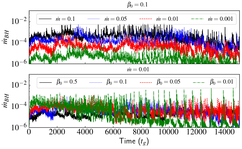
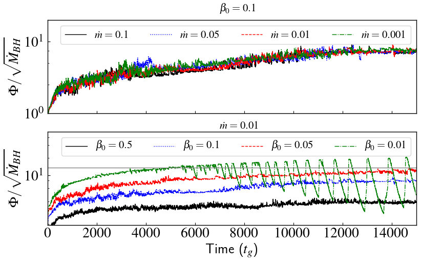
Figure 1: Plot of accretion rate measured at the event horizon$(\dot{M}_{\rm BH})$ profiles (left) and normalised magnetic flux $(\Phi/\sqrt{\dot{M}_{\rm BH}})$ around the event horizon profiles (right) as a function of simulation time (in units of $t_{g}$) for different simulation models. The upper panels show accretion rate profiles by varying input accretion rates, while lower panels show accretion rate profiles by varying magnetic field strength ($\beta_{0}$). The thin horizontal line in the left figure corresponds to $\Phi/\sqrt{\dot{M}_{\rm BH}}=15$.

In this section, we study the long-term temporal behaviour of our simulation models. In Fig. 1, we plot the accretion rate profiles measured at the event horizon in Eddington units $(\dot{m}_{\rm BH}=\dot{M}_{\rm BH}/\dot{M}_{\rm Edd})$ (left) and normalised magnetic flux $(\Phi/\sqrt{\dot{M}_{\rm BH}})$ profiles around the event horizon (right) for different simulation models, where $\dot{M}_{\rm BH}$ refer to accretion rate calculated at the event horizon of the black hole. In the upper panels, we show variation with accretion rates with a fixed value of input plasma-$\beta$ parameter $(\beta_{0}=0.1$, marked on the top of the figure), while the lower panels show variations with magnetic field strength ($\beta_{0}$) for a fixed accretion rate ($\dot{m}=0.01$, marked on the top of the figure). In the lower-left panel, we mark $\Phi/\sqrt{\dot{M}_{\rm BH}}=15$ with a horizontal line. We observe that the accretion rate profile in all our simulation models shows a quasi-steady behaviour with time, except for model G ($\beta_{0}=0.01,\dot{m}=0.01)$. In model G, the accretion rate profile initially reaches a quasi-steady state, but after a simulation time $t>6000\,t_{g}$, the accretion rate profile shows sporadic oscillations. These oscillations are similar to the ones observed by Dihingia et al. (2021).

With the increase of the input accretion rate ($\dot{m}$), the accretion rate profiles show quite a similar trend. Although due to different normalisation factors, the average value in Eddington units increases with the input accretion rate parameter $(\dot{m})$. The normalised magnetic flux around the horizon $\Phi/\sqrt{\dot{M}_{\rm BH}}$ profiles is insensitive to the input accretion rate ($\dot{m}$). All the models in panel (b) show a monotonically increasing behaviour with time, and after $t\gtrsim 10000\,t_{g}$, the profiles saturate with $\Phi/\sqrt{\dot{M}_{\rm BH}}\sim 8$.

With the increase of magnetic field strength (decreasing of $\beta_{0}$), the quasi-steady value of the accretion rate increases. Strong magnetic fields can facilitate stronger disc winds and consequently help in angular momentum transport, which results in a higher rate of mass flux to the black hole (Dihingia et al., 2021). With the decrease of input $\beta_{0}$, the $\Phi/\sqrt{\dot{M}_{\rm BH}}$ shows scaling behaviour, except for $\beta_{0}=0.01$ (model G). For all the other models, the value of $\Phi/\sqrt{\dot{M}_{\rm BH}}$ saturates after simulation time $t\gtrsim 10000\,t_{g}$. The saturation values for $\beta_{0}=0.5,0.1,$ and $0.05$ is $\Phi/\sqrt{\dot{M}_{\rm BH}}\sim 2.5,8$, and $13$, respectively. However, for model G ($\beta_{0}=0.01$, green line), the value of normalised magnetic flux exceeds $\Phi/\sqrt{\dot{M}_{\rm BH}}=15$ (see the horizontal line in panel d) after simulation time $t\gtrsim 4000\,t_{g}$. After that, we observe large oscillatory behaviour in the magnetic flux profile, which signifies magnetically arrested disc (MAD, (Tchekhovskoy et al., 2011)) configuration. During MAD, we also observe similar oscillations in the accretion rate profile for the same simulation model (see green line in panel c). Thus, all other simulation models do not develop MAD configurations; they are known as in standard and normal evolution (SANE) configurations.

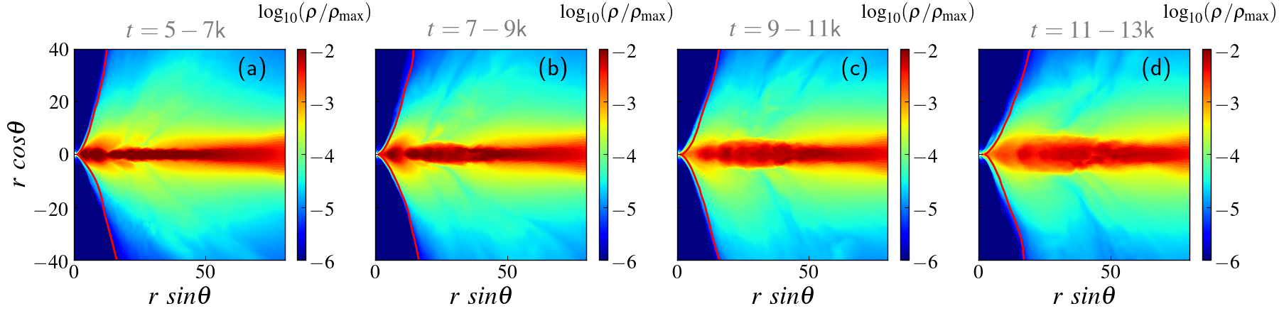
Figure 2: Distribution of time-averaged logarithmic normalised density distribution $(\log_{10}(\rho/\rho_{\rm max}))$ for the reference model (model C) on the poloidal plane for different simulation times, marked on the top of the figure. The solid red line corresponds to $\sigma=1$ contour.

4 Density distribution

In Fig. 2, we show the time-averaged logarithmic normalised density distribution of $(\log_{10}(\rho/\rho_{\rm max}))$ for different simulation times for the reference model (model C), where we consider the input accretion rate $\dot{m}=0.01$ and input plasma-$\beta$ parameter $\beta_{0}=0.1$. The red solid contour in the panels represents the boundary of $\sigma=b^{2}/\rho=1$. Panels (a), (b), (c), and (d) correspond to the distribution calculated between simulation times $t=5000-7000\,t_{g}$, $7000-9000\,t_{g}$, $9000-11000\,t_{g}$, and $11000-13000\,t_{g}$, respectively. The quasi-steady structure of the accretion disc can be divided into three major parts: (i) high-density thin-disc around the equatorial plane; (ii) low-density off-equatorial region; and (iii) very low-density funnel region. The low-density region contributes to the disc winds, and the very low-density region around the polar axis contributes to the relativistic Poynting-dominated jet (see Vourellis et al., 2019; Dihingia et al., 2021). In order to understand the time evolution of disk structure better, we plot the contours of the edge of high-density region ($\rho/\rho_{\rm max}=0.01$) at different time range in Fig. 3, where black, red, blue, green, and magenta lines correspond to $\rho/\rho_{\rm max}=0.01$ at time-averaged over $t=5000-7000\,t_{g}$, $7000-9000\,t_{g}$, $9000-11000\,t_{g}$, $11000-13000\,t_{g}$, and $13000-15000\,t_{g}$, respectively. The figure clearly demonstrates that with time, the matter in the high-density thin disc spreads to the off-equatorial plane, and the disc-thickness increases. It also shows that close to the black hole, the flow forms a mini-torus-like structure during its evolutionary phase.

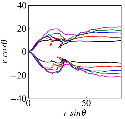
Figure 3: Plot of time-averaged high-density contours $(\rho/\rho_{\rm max}=0.01)$ for the reference model at time $t=5000-7000\,t_{g}$ (black), $7000-9000\,t_{g}$ (red), $9000-11000\,t_{g}$ (blue), $11000-13000\,t_{g}$ (green), and $t=13000-15000\,t_{g}$ (magenta), respectively.

The structure of the disc may also depend on the other flow parameters. Here, in this section, we study the disc structure with input accretion rate and magnetic field strength (input plasma-$\beta$ parameter, i.e., $\beta_{0}$). In Fig. 4, we show the time-averaged logarithmic normalised density distribution of $(\log_{10}(\rho/\rho_{\rm max}))$ for the cases with different input accretion rates $(\dot{m})$ and different input plasma-$\beta$ parameters $\beta_{0}$. The time averaging is computed over a simulation time $t=13000-15000\,t_{g}$, and the values of $\dot{m}$ and $\beta_{0}$ are marked on the top of the panels. The red solid contours represent the boundary of $\sigma=b^{2}/\rho=1$. For the upper panels, we consider $\beta_{0}=0.1$ and for the lower panels, we consider $\dot{m}=0.01$. In the upper panels, we study the role of accretion rate on the disc structure (Fig. 4a-d).

With the increase of the input accretion rate, the radiative cooling efficiency increases, which leads to a cooler thin disc. As a result, we observe a thinner high-density region for higher accretion rate cases (Fig. 4a-d). In the lower panels of Fig. 4, we study the role of the magnetic field strength on the disc structure. With the increase of the magnetic field strength (Fig. 4e-h), the matter in the thin disc reduces drastically due to the strong disc winds (which will be discussed in upcoming sections). By comparing panels of Fig. 4e and f, we see that due to the higher magnetic pressure in the disc, the disc thickness increases. Moreover, in panels Fig. 4g and h, the density close to the equatorial plane is reduced by orders of magnitude.

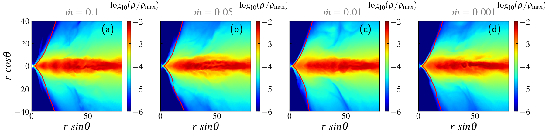
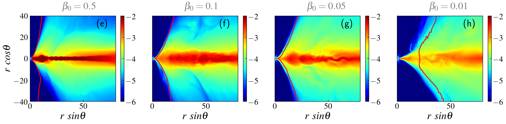
Figure 4: Distribution of time-averaged ($t=13000-15000\,t_{g}$) logarithmic normalised density $(\log_{10}(\rho/\rho_{\rm max}))$ on the poloidal plane for simulation models with different accretion rates (top) and for different magnetic field strengths through $\beta_{0}$ (bottom). The solid red line corresponds to $\sigma=1$ contour.

In summary, we found that accretion rate and magnetic field strength play a vital role in the evolution of the thin-disc structure. In the following sections, we investigate their effects in great detail and their applications in understanding the physics around BH-XRBs.

5 Properties of temperatures

The radiative properties of an accretion disc have a direct correlation with the temperature of the fluid, particularly the electron temperature. In this section, we study the properties of the electron and ion temperatures of the accretion flow. To do that, we plot logarithmic dimensionless time-averaged (over $t=13000-15000\,t_{g}$) electron temperature $\Theta_{e}=k_{\rm B}T_{e}/m_{e}c^{2}$ in Fig.  5 follows the same fashion as Fig.  4. The solid red line in the figure depicts the boundary for $\Theta_{e}=1$. In all the panels, we see that electrons are hotter in the jet-sheath/corona region due to the strong turbulent heating in these regions ($\Theta_{e}\gtrsim 10$, see the bright white-yellow region in Fig. 5). In other regions of the simulation domain, the electron temperature is always smaller ($\Theta_{e}\lesssim 1$). With the increase of the input accretion rate $(\dot{m})$, the overall density of the flow increases, which results in higher cooling efficiency for all the radiative processes. Accordingly, electrons are cooler for higher accretion rate models (see upper panels of Fig. 5). For models with a lower accretion rate ($\dot{m}=0.01,0.001$), the electrons close to the equatorial plane but far from the black hole are comparatively hotter as compared to the models with a higher input accretion rate $(\dot{m}=0.1,0.05)$ (compare panels Fig. 5(a,b) and Fig. 5(c,d)). For example, for the case with $\dot{m}=0.01$, electrons at the equatorial plane have a temperature of $\Theta_{e}\sim 0.3$. However, for the case with $\dot{m}=1.0$, electrons at the equatorial plane have a temperature of the order of $\Theta_{e}\sim 0.03$, which is around ten times smaller. Such a low electron temperature around the equatorial plane essentially suggests the importance of radiative cooling due to the optically-thick black body component in these ranges of accretion rates ($\dot{m}\gtrsim 0.5$).

Although, with the increase of the magnetic field strength, the emission due to synchrotron radiation also increases. However, in Fig. 5, it is shown that electrons become hotter for models with lower initial $\beta_{0}$ (stronger magnetic field). This essentially suggests that the turbulent heating present in the flow is much more efficient than that of radiative cooling. Consequently, we see that the area under the $\Theta_{e}=1$ contour increases with the increasing magnetic field strength (lowering $\beta_{0}$). For higher initial $\beta_{0}$ cases, the electrons away from the equatorial plane surrounding the corona region are cooled ($\Theta_{e}\lesssim 0.01$, see the dark black region of the panels Fig. 5e, 5f, and 5g). With the increase of the magnetic field strength $(\beta_{0}=0.01)$, the electron temperature in this region increases by orders of magnitude ($\Theta_{e}\sim 0.3$, see the reddish region of the panel Fig. 5h).

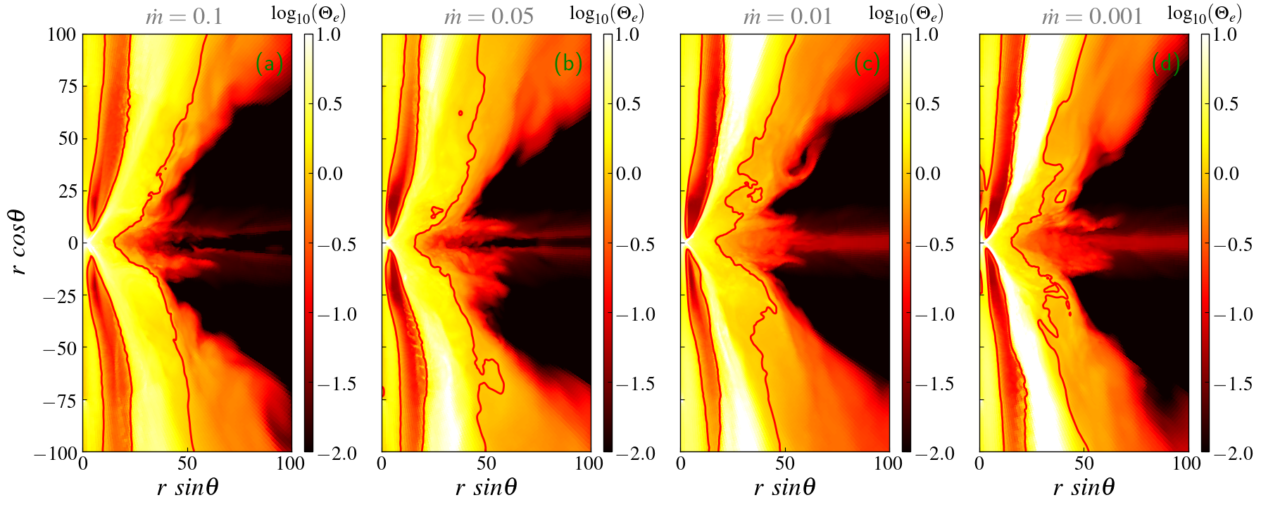
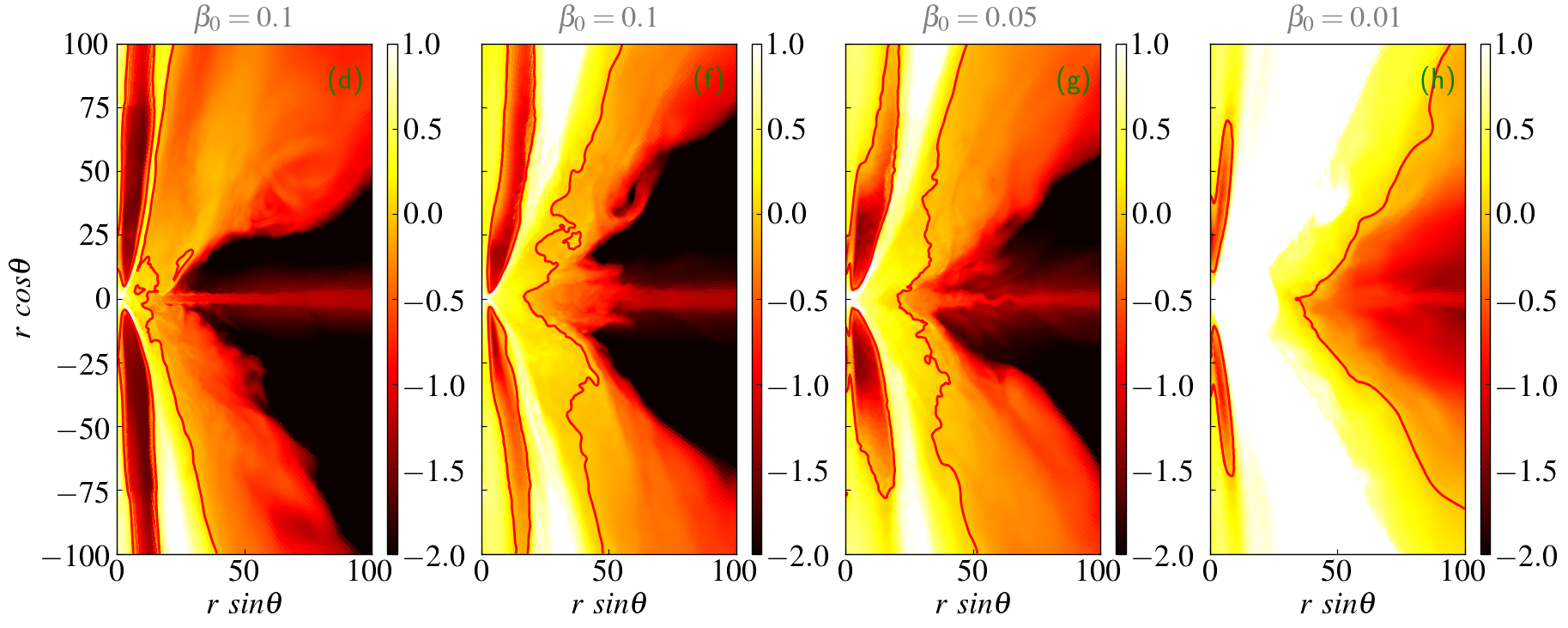
Figure 5: Same as Fig. 4, except showing the dimensionless electron temperature $\log_{10}(\Theta_{e})$. The solid red line corresponds to $\Theta_{e}=1$ contour.

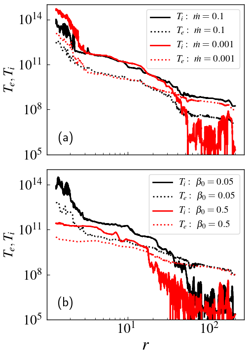
Figure 6: The comparison of dimensional electrons and ions temperatures ($T_{i},T_{e}$, in Kelvin) for different (a) input accretion rates (upper panel) and (b) input plasma-$\beta$ parameters ($\beta_{0}$, lower panel) is shown on the equatorial plan. The solid lines represent ion temperature, whereas the dotted lines represent electrons temperature.

To study the temperature profiles in the thin disc, we compare the time-averaged temperatures of electrons and ions ($T_{e},T_{i}$, in Kelvin) for various accretion rates (upper panel) and initial plasma-$\beta$ (lower panel) parameters on the equatorial plane in Fig. 6. The time averaging for the temperatures are taken at simulation times between $t=13000-15000\,t_{g}$. In the upper panel, we fixed initial plasma-$\beta$ at $\beta_{0}=0.1$, while in the lower panel, we fixed the input accretion rate at $\dot{m}=0.01$. In the figure, the solid and dotted lines represent ion and electron temperatures, respectively. In Fig. 6a, for the lower accretion rate (red lines), far from the black hole ($r>30\,r_{g}$) electrons are hotter than ions, which is due to inefficient electron cooling mechanisms. With the increase in accretion rate, the electrons cool efficiently due to the optically thick component of the radiation, and as a result, the electrons become cooler than the ions (see the black lines). However, in the intermediate radii ($2\,r_{g}\lesssim r\lesssim 30\,r_{g}$) the temperatures of the electrons and ions do not significantly depend on the accretion rates. On the other hand, in the region near the black hole $(r\lesssim 2\,r_{g})$, the temperatures of electrons and ions are lower for higher accretion cases due to higher Bremsstrahlung and Coulomb heating processes. It is interesting to note that the ion and electron temperatures close to the black hole reach as high as $T_{i}\sim 10^{14}$K and $T_{e}\sim 10^{12}$K.

Figure 6b shows that for the weak magnetic field case ($\beta_{0}=0.5$), the temperatures of electrons and ions are much smaller close to the black hole as compared with the high magnetic field case ($\beta_{0}=0.05$). The maximum ion temperature is of the order of $T_{i}\sim 10^{14}$K and $T_{i}\sim 10^{11}$K for $\beta_{0}=0.05$ and $\beta_{0}=0.5$, respectively. Similarly, the maximum electron temperature is of the order of $T_{e}\sim 10^{12}$ and $T_{e}\sim 5\times 10^{9}$K for $\beta_{0}=0.05$ and $\beta_{0}=0.5$, respectively. These facts essentially suggest the importance of the turbulent heating process in deciding the temperature of both the electrons and ions. The impacts of the initial plasma-$\beta$ parameters can be seen throughout the length scale of the accretion disc. Even far from the black hole ($r>20\,r_{g}$ for $\beta_{0}=0.5$ and $r>30\,r_{g}$ for $\beta_{0}=0.05$), electrons remain hotter than ions for both the magnetic field limits.

In a similar spirit as in Fig. 4, Fig.  8 shows the distribution of the time-averaged (over $t=13000-15000\,t_{g}$) the ratio between dimensional electron and ion temperatures as $\log_{10}(T_{e}/T_{i})$, where the boundary of $T_{e}/T_{i}=1$ is represented as a solid black curve. The ratio $T_{e}/T_{i}$ essentially depicts the distribution of thermal energy of the fluid over electrons and ions. In the corona region, the thermal energy of the electron is always lower than that of the ion thermal energy ($T_{e}/T_{i}<1$). The effects of the increasing radiative cooling with the accretion rate can be seen in the upper panels of figure 8. For a higher accretion rate, the thermal energy of electrons is lower than that of ions in the thin-disc region (see the blue region in Fig. 8a and 8b). However, for a lower accretion rate, the thermal energy of the electron remains higher than that of the ions in the thin-disc region. Away from the corona region, the thermal energy of ions is always higher than that of electrons (see the red region in Fig. 8a-8h).

The ratio $T_{e}/T_{i}$ shows a non-monotonic behaviour with the increase of the magnetic field strength (lowering $\beta_{0}$, Fig. 8e-8h). Initially, with the increase of the magnetic field strength, the emission due to the Synchrotron radiation increases. The electron loses its thermal energy. As a result, the area with $T_{e}/T_{i}<1$ in the corona region increases, and also the ratio $T_{e}/T_{i}$ decreases (see the darker blue color in panel Fig. 8g as compared to panel 8f). However, with a further increase in the magnetic field strength, the turbulent heating efficiency also increases, leading to an increase in the ratio of $T_{e}/T_{i}$ in the corona. With this, the ratio of temperatures becomes greater than unity ($T_{e}/T_{i}>1$) in some parts of the corona region (see Fig. 8h).

5.1 Temperatures with heating prescriptions

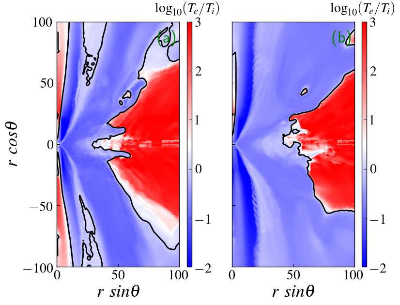
Figure 7: Distribution of time-averaged temperatures ratio ($\log_{10}(T_{e}/T_{i}$)) for (a) turbulent heating (model C) and (b) reconnection heating (model C-R) for electrons. The black solid line represents the boundary of $T_{e}/T_{i}=1$.

In this section, we study the impact on the ratio of temperatures ($T_{e}/T_{i}$) with different heating prescriptions for electrons. Accordingly, in Fig. 7, we show the time-averaged (over $t=13000-15000\,t_{g}$) distribution of $T_{e}/T_{i}$ for two heating prescriptions (a) turbulent heating (Howes, 2010, 2011) and (b) reconnection heating (Rowan et al., 2017), i.e., for model C and model C-R, respectively. For both the models, the input accretion rate and the initial magnetic flux strength are fixed to $\dot{m}=0.01$ and $\beta_{0}=0.1$, respectively. The figure essentially suggests that the electrons in the funnel region are mostly cooler than the ions for the reconnection heating model, implying the inefficiency of reconnection heating in the highly magnetised regions. Whereas, for the turbulent heating model, we observe a significant area with $T_{e}/T_{i}>1$ around the funnel region. Also, the area with $T_{e}/T_{i}<1$ is also significantly bigger for the reconnection heating model as compared to the turbulent heating model. However, the region with $\beta\ll 1$ above the thin remains $T_{e}/T_{i}>1$ for both the heating prescriptions.

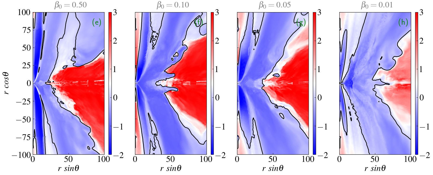
Figure 8: Same as Fig. 4, except showing the ratio between dimension-full electron and proton temperatures in $\log_{10}(T_{e}/T_{i})$. A solid black line corresponds to $T_{e}/T_{i}=1$ contour.

5.2 Correlation of $T_{e}/T_{i}$ with plasma-$\beta$

In this section, we focus on the correlation between the ratio of temperatures ($T_{e}/T_{i}$) and the flow plasma-$\beta$ profile. In previous study, Dihingia et al. (2023) proposed a $R-\beta$ ansatz that provides the trend of $T_{e}/T_{i}$ with flow plasma-$\beta$ in the presence of radiative cooling and heating, which is given by,

$$\frac{T_{i}}{T_{e}}=\frac{1}{1+\beta^{2}}R_{1}+\frac{\beta^{2}}{1+\beta^{2}}R_{2}+\frac{\beta}{\beta+\beta_{{\rm br}}}R_{3}\,,$$ (18)

where $R_{1-3}$ are constant determining the nature of $T_{i}/T_{e}$ in different ranges of plasma-$\beta$. For, $\beta\ll 1$ the ratio becomes $T_{i}/T_{e}=R_{1}$, whereas for $\beta\gg 1$ the ratio becomes $T_{i}/T_{e}=R_{2}+R_{3}$. Note that this ansatz recovers the form of the $R-\beta$ relation provided by Mościbrodzka et al. (2016) when $R_{3}=0$. In that case, $R_{1}=R_{\rm low}$ and $R_{2}=R_{\rm high}$, i.e.,

$$\frac{T_{i}}{T_{e}}=\frac{R_{\rm low}}{1+\beta^{2}}+\frac{R_{\rm high}\beta^{2}}{1+\beta^{2}}\,.$$ (19)

Recently, Meringolo et al. (2023) also proposed such a relation between the temperature ratio, the plasma-$\beta$, and magnetisation $(\sigma)$ with kinetic Particle-In-Cell (PIC) simulations, which is given by,

$$\frac{T_{i}}{T_{e}}=\left[t_{0}+t_{1}\sigma^{\tau_{1}}\tanh\left[t_{2}\beta\sigma^{\tau_{2}}\right]+t_{2}\sigma^{\tau_{3}}\tanh\left[t_{3}\beta^{\tau_{4}}\sigma\right]\right]^{-1}\,.$$ (20)

where $t_{0}=0.4$, $t_{1}=0.25$, $t_{2}=5.75$, $t_{3}=0.037$, $\tau_{1}=-0.5$, $\tau_{2}=0.95$, $\tau_{3}=-0.3$, and $\tau_{4}=-0.05$. In Dihingia et al. (2023), we consider the accretion flow to be geometrically thick (torus), and such accretion flows are applicable around low-luminous AGNs. However, here we study a geometrically thin disc, and therefore, we want to study the possibility of a similar correlation between the ratio of temperatures and the plasma-$\beta$ profile.

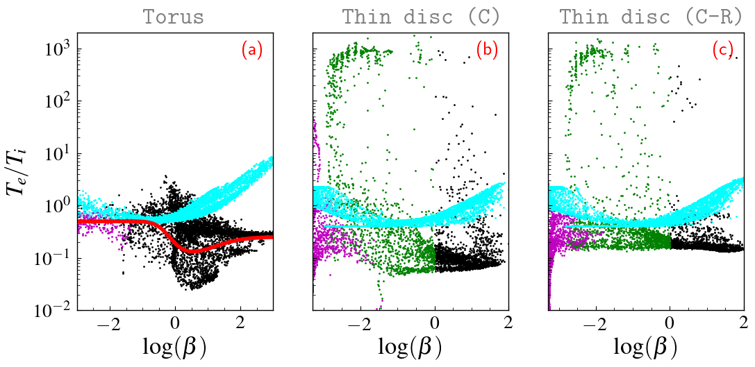
Figure 9: Distributions of the time-averaged temperatures ratio $T_{e}/T_{i}$ as a function of plasma-$\beta$ for geometrically (a) thick, (b) thin accretion flow (model C), and (c) thin accretion flow (model C-R). Each dot refers to a cell in the computational domain, with the black dots referring to the region with $\sigma<1$ and the magenta dots to the region with $\sigma>1$ (roughly representative of the jet). The cyan dots represent temperature ratios using Eq. 20. The solid red curves correspond to $R-\beta$ relations.

In order to fully understand the differences in the correlation in these two scenarios (torus and thin disc), in Fig. 9, we collect the time-averaged ratio of the temperatures $T_{e}/T_{i}$ from all the grid-cells in the computational domain with $r<100\,M$. The distribution for torus is shown in the panel Fig. 9a and the distribution for thin-disc is shown in Fig. 9b and 9c. Panel 9b show the correlations of temperatures for model C and in panel 9b show the correlations of temperatures for model C-R. The black and magenta dots refer to the ratio collected from the region with $\sigma<1$ and $\sigma>1$ (roughly representative of the jet) region, respectively. For the torus, we use the model TRC-A of the Dihingia et al. (2023) and for the thin disc, we consider our reference model (model C). The panels essentially suggest that the ratio $T_{e}/T_{i}$ behaves in quite a different manner. For the torus case, it is possible to fit all the data roughly with Eq. 18, which is shown by the red solid line. However, for the thin disc case, some data points have a much larger temperature ratio, $T_{e}/T_{i}\gg 1$ in the range between $10^{-3}\leq\beta\leq 10^{-1}$. Due to the presence of these data points, it is impossible to fit the data using Eq. (18). Consequently, we avoid doing it. The cyan dots represent the temperature ratios calculated using Eq. (20). We observe that the cyan dots overlap with the simulated temperature ratios in the simulation domain for highly magnetised region $(\beta\ll 1)$. However, in the low magnetised region, the relation provided by Meringolo et al. (2023) does not provides good agreement.

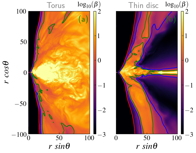
Figure 10: Distribution of flow plasma-$\beta$ profile for torus (a) and thin-disc (b) simulation. The red, green, and blue lines represent the boundary of $\sigma=1$, $\beta=1$, and $\beta=0.1$, respectively.

Figure 10 shows the plasma-$\beta$ distribution for both torus and thin-disc models, where the red, green, and blue lines represent the boundary of $\sigma=1$, $\beta=1$, and $\beta=0.1$, respectively. For the torus model (Fig. 10a), the plasma-$\beta$ is mostly greater than that of unity except in the relativistic jets ($\sigma>1$ region), i.e., the flow is mostly gas pressure dominated. For the thin-disc model (Fig. 10b), we see that around the equatorial plane, the flow is gas pressure dominated $\beta\gg 1$, as the flow moves away from the equatorial plane, it becomes magnetic pressure dominated ($\beta<1$, see the dark region of the Fig. 10b). However, around the rotation axis (jet and corona) of the black hole, the distribution of plasma-$\beta$ is quite similar to the torus setup. Thus, the scenario of plasma-$\beta$ distribution is completely different for the thin-disc due to the presence of the low-$\beta$ region between the thin-disc and the corona. This low-$\beta$ region essentially represents the Blandford & Payne (1982) dominated disc-wind (see next section for details). In summary, in the case of magnetised thin-disc, the simplified $R-\beta$ prescription can not reproduce the trend of electron-to-ion temperature ratio ($T_{i}/T_{e}$) in terms of flow plasma-$\beta$. Accordingly, in such a scenario, a two-temperature framework is unavoidable for a proper description of electron temperature.

6 Properties of disc-winds

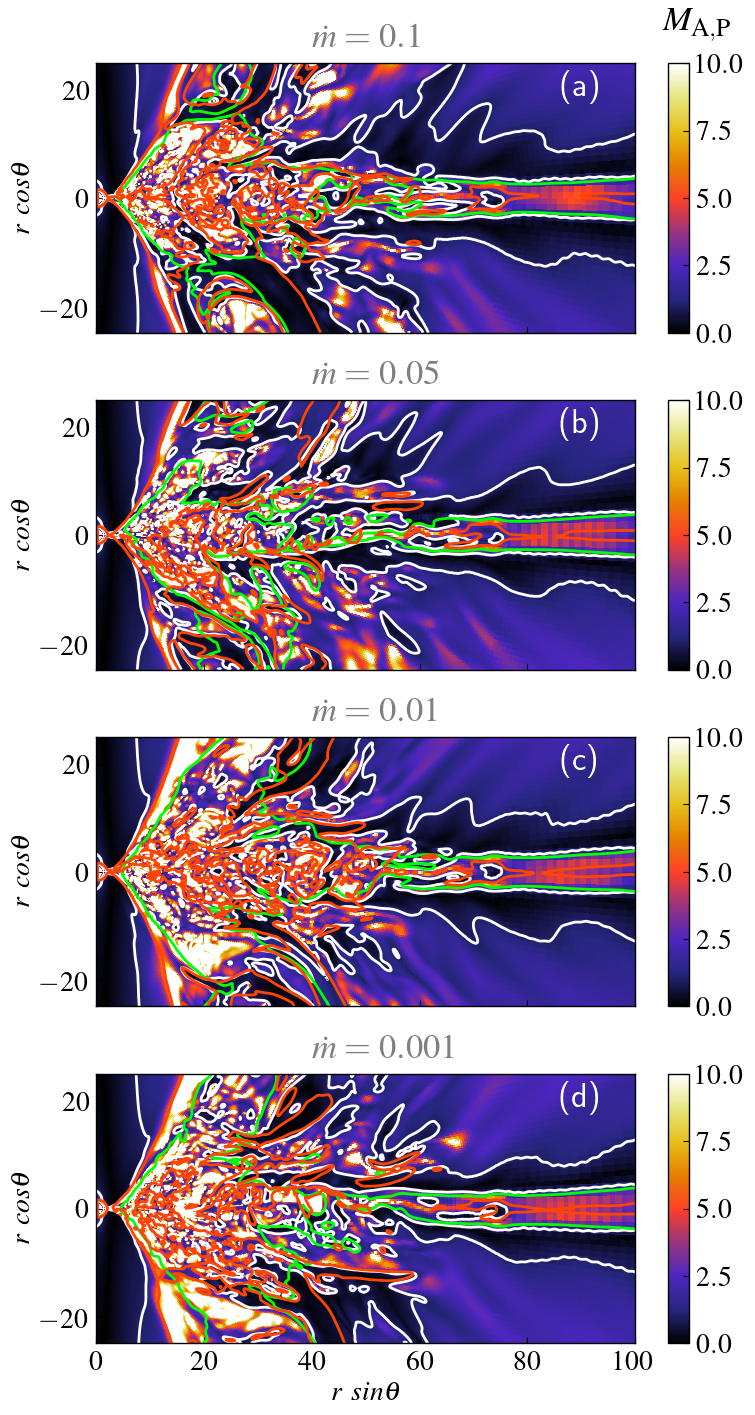
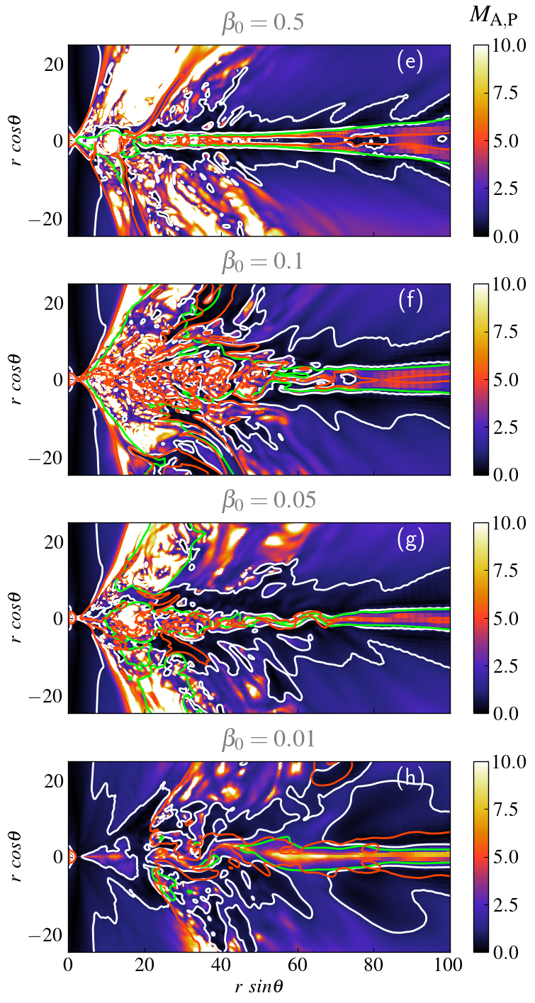
Figure 11: Distribution of Alfvénic Mach number $(M_{\rm A,P})$ for different accretion rates (left panels (e)-(h)) and magnetic field strengths (right panels, (e)-(h)). The white, green, and red lines correspond to the boundaries of $M_{\rm A,P}=1$, $\beta=1$, and $B_{\rm tor}/B_{p}=5$, respectively.

In this section, we characterize different types of disc winds from the accretion disc and subsequently investigate the role of flow parameters in the launching of disc winds in the presence of radiative cooling and electron heating. To do that, in Fig. 11, we show the distribution of Alfvénic Mach number $(M_{\rm A,P})$ for the different input accretion rates (left panels (e)-(h)) and the magnetic field strengths (right panels, (e)-(h)). The values of input accretion rates $(\dot{m})$ and the initial plasma-$\beta$ parameters ($\beta_{0}$) are given at the top of each panel. The white, green, and red lines correspond to the boundaries of $M_{\rm A,P}=1$, $\beta=1$, and $B_{\rm tor}/B_{p}=5$, respectively. The poloidal Alfvénic Mach number is obtained as $M_{\rm A,p}=u_{p}/c_{a}$, where $h=1+\frac{\Gamma p}{(\Gamma-1)\rho}$, $c^{2}_{\rm a}=B_{p}^{2}/(\rho h+B_{p}^{2})$, $u_{p}^{2}=[u^{r}u_{r}+u^{\theta}u_{\theta}]_{\rm BL}$, and finally $B_{p}^{2}=[B^{r}B_{r}+B^{\theta}B_{\theta}]_{\rm BL}$. Following a similar procedure, the toroidal component of the magnetic fields is calculated as $B^{2}_{\rm tor}=[B^{\phi}B_{\phi}]_{\rm BL}$. The subscript BL indicates that the quantities are calculated at Boyer-Lindquist coordinates.

In all the cases, the region around the rotation axis of the black hole flow is always sub-Alfvénic Mach number. In this region $\beta\ll 1$ and $B_{\rm tor}/B_{p}\ll 1$, which indicated the presence of magnetically driven relativistic jet. Surrounding that, we observe a region with super-Alfvénic Mach number. In this region $M_{\rm A,p}\gg 1$, $\beta\gtrsim 1$, and $B_{\rm tor}/B_{p}\gg 1$. It signifies the $B_{\rm tor}$ dominated disc-wind. The launching mechanism for this component of the disc-wind is the gradient of magnetic pressure due to the toroidal component of the magnetic field (e.g., Vourellis et al., 2019; Dihingia et al., 2021). $B_{\rm tor}$ dominated disc-wind is often hot and acts as a hot disc-wind corona around the black hole. Also, plasmoids can be seen in this region (Dihingia et al., 2021).

Far from the black hole, the accretion flow has $M_{\rm A,p}>1$ (super-Alfvénic), $\beta\gg 1$, and $B_{\rm tor}/B_{p}\gtrsim 1$ around the equatorial plane. However, away from the equatorial plane, flow becomes sub-Alfvénic $M_{\rm A,p}<1$, with $\beta\ll 1$ and $B_{\rm tor}/B_{p}>5$. Moreover, flow again becomes super-Alfvénic $M_{\rm A,p}>1$ as it moves far from the equatorial plane. These facts strongly suggest the presence of Blandford & Payne (1982) disc wind (BP disc-wind).

In left panels of Fig. 11a-11d, we study the variation of the signature of $B_{\rm tor}$ and BP disc-wind for different accretion rates. When accretion rates increase, the radiative cooling rates are larger and the flow becomes much cooler. As a result, the disc-wind corona becomes less turbulent, and thereby the toroidal component weakens. Thus, we see that the area of $B_{\rm tor}$ dominated disc wind decreases with the increase of the accretion rate (see the bright region of the panels Fig. 11a-11d). On the other hand, due to the cooler flow close to the equatorial plane (thin-disc), the poloidal component of the magnetic field can be sustained better. As a result, the area of BP disc wind increases with the increase in the input accretion rate (see the dark region of the panels Fig. 11a-11d).

In the right panels of Fig. 11e-11h, we study the role of magnetic field strength on the signature of $B_{\rm tor}$ and BP disc wind. In a previous study, Dihingia et al. (2021) reported that the stronger magnetic fields are more susceptible to BP disc wind, whereas they are less susceptible to $B_{\rm tor}$ disc wind. In our simulations, we also observe that the area of $B_{\rm tor}$ dominated disc-wind decreases with the increase of magnetic field strength (lowering $\beta_{0}$, see the bright white region). On the other hand, the area of BP disc wind increases with the increase of magnetic field strength (lowering $\beta_{0}$, see the dark region). Thus, with the inclusion of radiative cooling and heating, we do not find any qualitative alteration of the results reported by Dihingia et al. (2021). It indicates that disc wind properties do not depend on radiative cooling and heating. However, depending on the radiative cooling and heating, the dominant components of the disc winds can be different.

6.1 Disc wind rates

To determine the quantitative behaviour of the disc-winds, in Fig. 12, we present the poloidal mass flux $(\dot{m}_{p}=\sqrt{-g}\rho u_{p}$, in code units) as a function of radii at an angle of $\theta=75^{\circ}$. In the upper panel, we plot $\dot{m}_{p}$ for different values of input accretion rates ($\dot{m}$) for fixed $\beta_{0}=0.1$ and in lower panel, we plot $\dot{m}_{p}$ for different values of input plasma-$\beta$ parameters ($\beta_{0}$) for a fixed value of $\dot{m}=0.1$. The figures essentially show two distinct components of the disc winds, $B_{\rm tor}$ dominated disc-wind and the BP-dominated disc-wind. For radii $r<50\,r_{g}$, the mass flux shows turbulent behavior suggesting $B_{\rm tor}$ dominated disc-wind. On the other hand, $r>50\,r_{g}$, the poloidal mass flux is stable, suggesting the BP-dominated disc-wind (see the vertical line in Fig.  12).

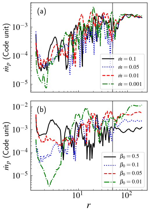
Figure 12: Plot of poloidal mass flux $(\dot{m}_{p}=\sqrt{-g}\rho u_{p})$ for different values of (a) input accretion rates ($\dot{m}$, upper panel) and (b) input plasma-$\beta$ parameters ($\beta_{0}$, lower panel). The vertical line in the panels refers to $r=50\,r_{g}$.

For different values of the accretion rates ($\dot{m}$), the poloidal mass flux profiles are quite similar. Thus, the mass flux scales linearly with the accretion rate. However, with the increase of magnetic field strength (lowering $\beta_{0}$), the poloidal mass flux increases due to the presence of BP disc wind. We see that while decreasing from $\beta_{0}=0.5$ to $\beta_{0}=0.01$, BP mass flux increases from $\dot{m}_{p}\sim 10^{-4}$ to $\dot{m}_{p}\sim 10^{-3}$.

7 Radiative properties

In this section, we investigate the radiative properties of the thin disc and the impacts of input accretion rate and magnetic field strength on them. To do that, we calculate light curves at different emitted frequencies using general-relativistic radiative transfer (GRRT) code BHOSS (Younsi et al., 2012; Younsi et al., 2020; Younsi et al., 2023). For our calculation, we consider the emission from bremsstrahlung, thermal synchrotron, and black body radiation following (Rybicki & Lightman, 1979; Leung et al., 2011; Page & Thorne, 1974), respectively. Accordingly, we show the comparison of the total flux (in Jansky (Jy)) at frequencies $\nu=10^{14},10^{17}$ and $10^{19}$Hz for different accretion rates in Fig. 13. Black, blue, and red lines correspond to light curves at accretion rate $\dot{m}=0.1,0.01$, and $0.001$, respectively. These frequencies are chosen in such a way that for the frequency $\nu=10^{14}$Hz, the synchrotron process dominates. For $\nu=10^{17}$ Hz, the black body component dominates, and for $\nu=10^{19}$Hz, either synchrotron or bremsstrahlung dominates. At frequency $\nu=10^{14}$Hz, the average value of the photon flux for accretion rates $\dot{m}=0.1,0.01$, and $0.001$ are $<F(\nu=10^{14})>=0.016,8.8\times 10^{-4},$ and $7.9\times 10^{-6}$ Jy, respectively. The temporal properties show a very small variability pattern at the frequency. At frequency $\nu=10^{17}$Hz, the average value of the flux for accretion rate $\dot{m}=0.1,0.01$, and $0.001$ are $<F(\nu=10^{17})>=0.028,4.6\times 10^{-4},$ and $4.4\times 10^{-6}$ Jy, respectively. The temporal properties of the light curves at this frequency for different accretion rates do not show any variability as these fluxes are mostly coming from the black body radiation, which comes from the steady equatorial part of the flow. At frequency $\nu=10^{19}$Hz, we observe quite a similar feature as compared to frequency $\nu=10^{17}$Hz, with a more prominent variability pattern. The average value of the photon flux at this frequency for accretion rates $\dot{m}=0.1,0.01$, and $0.001$ are $<F(\nu=10^{19})>=9.4\times 10^{-6},5.4\times 10^{-8},$ and $8.1\times 10^{-11}$ Jy, respectively. However, the light curves at the lower end are smoothed out for accretion rates $\dot{m}=0.01$, and $0.001$, essentially suggesting that the emission from the Bremsstrahlung process is higher than that of the Synchrotron process at this frequency. We also note that the emission from Bremsstrahlung does not vary significantly with time, as the Bremsstrahlung radiation is emitted only from the high-density thin-disc region, which remains dynamically steady throughout the simulation time. On the other hand, high-energy synchrotron radiation is emitted mostly from the disc-wind region, which is turbulent in nature. As a result, synchrotron-dominated light curves are much more variable (see the next section for detail).

Figure 14 shows the comparison of light-curves for different initial plasma-$\beta$ ($\beta_{0}$) parameters at frequencies ($\nu=10^{14},10^{17},$ and $10^{19}$Hz. We see that for weak magnetic field limit ($\beta_{0}=0.5$), the photon flux in all frequencies is very small as compared to moderate ($\beta_{0}=0.1$) and strong magnetic field limits ($\beta_{0}=0.01$). At frequency $\nu=10^{17}$Hz, the light curves for $\beta_{0}=0.5$ and $0.1$ is quite similar and steady, as for this magnetic field strength, the synchrotron emission is always weaker than that of the black body component. However, for $\beta_{0}=0.01$, we observe a variable light curve with an average flux greater than that of the weak magnetic field cases. This suggests stronger synchrotron emission compared to the black body radiation. In the case of $\nu=10^{19}$Hz and $\beta_{0}=0.5$, the photon flux is very small $<F(\nu=10^{19})>\sim 10^{-12}$ and does not vary at all with time, which is dominated only by the Bremsstrahlung radiations. However, for other cases, the flux and the variability pattern increase with the increase of magnetic field strength (lowering $\beta_{0}$).

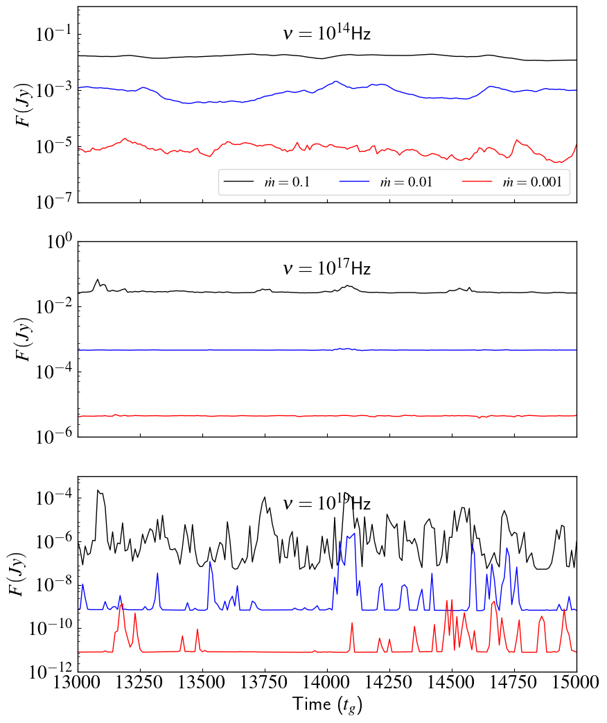
Figure 13: Plot of light-curves at frequencies $\nu=10^{14},10^{17}$ and $10^{19}$Hz for different values of the accretion rates $(\dot{m})$ marked on the figure.

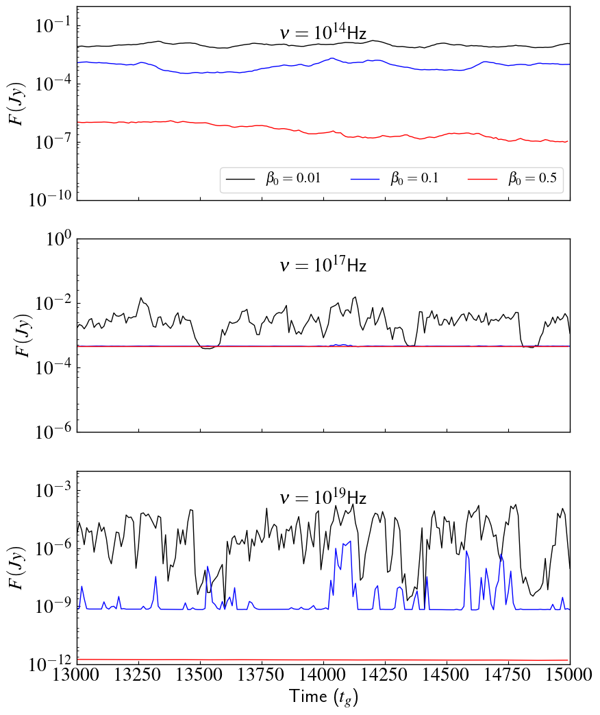
Figure 14: Plot of light-curves at frequencies $\nu=10^{14},10^{17}$ and $10^{19}$Hz for different values of the initial magnetic field strength $(\beta_{0})$ marked on the figure.

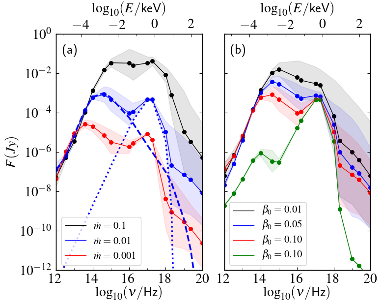
Figure 15: Plot of the time-averaged spectrum for different accretion rate (left, $\dot{m})$ and initial plasma-$\beta$ parameters (right, $\beta_{0})$. The shaded area shows the spread of the photon flux throughout the simulation time. The blue dashed and dotted lines in panel (a) correspond to the contributions from the synchrotron and the black body process.

7.1 Average spectra

To understand the impacts of the accretion rates and the initial plasma-$\beta$ parameters on the radiative properties throughout the energy range, in Fig. 15, we show the time-averaged spectra for different accretion rates (left, $\dot{m})$ and initial plasma-$\beta$ parameters (right, $\beta_{0})$. For the left figure, the initial plasma-$\beta$ is fixed with $\beta_{0}=0.1$ and for the right figure, the accretion rate is fixed as $\dot{m}=0.01$. In the figure, a shaded region indicates the spread of photon flux throughout the temporal domain ($t=13000-15000\,t_{g}$). In the top ‘x-axis’, for the benefit of readers, we show the photon energy $E=h\nu$ in terms of $\mathrm{keV}$. To understand the contribution of the individual emission processes, we overlay the contribution of the synchrotron and the black body in dashed and dotted lines for $\dot{m}=0.01$ case (blue colour) in Fig. 15a. Thus, the very low energy part ($E<\sim 0.1$keV) is dominated by the synchrotron emission, whereas the intermediate range $E\sim 0.1-10$keV is dominated by the black body component. The very high energy $E>\sim 10$keV is dominated by the bremsstrahlung process. All the spectra show the characteristic synchrotron peak around $\nu\sim 10^{15}-10^{16}$Hz frequency range. In the frequency range $\nu\sim 10^{16}-10^{18}$Hz ($\sim 0.1-10$keV), we observe the characteristic peak for the black body radiation. In the higher frequency range $\nu>10^{18}$Hz, we observe the characteristic signature of the Bremsstrahlung radiation, which is more prominent for lower accretion rates and weaker magnetic field strength.

With the increase of the accretion rate, the magnetic field strength increases due to the scaling relation. As a result, the synchrotron emission increases with the higher accretion rate. On the other hand, Bremsstrahlung emission also increases with the increase in density. Subsequently, in the figure, we see that the photon flux increases with the increase of the accretion rate. Also, the peak frequency of the radiation shifts towards the higher frequency range. Similarly, with the accretion rate, the peak due to the black body radiation also sifts towards the higher energy range with increases in flux in orders of magnitudes. For higher accretion rates, the high-energy tail at high frequency is also dominated by the synchrotron radiation due to the presence of a stronger magnetic field. However, the high-energy tail is dominated by the Bremsstrahlung radiation for lower accretion rates.

With the decrease of initial plasma-$\beta$ parameters, the magnetic field strength increases monotonically. Subsequently, the total magnetic flux increases with the decrease of $\beta_{0}$, and the peak synchrotron frequency shifts towards the higher frequency range. However, as the accretion rate is fixed, the black body component does not change at all with the increase in magnetic field strength. Nonetheless, in the case of lower magnetic field strength, dominating the emission process is black body radiation. With the increase in magnetic field strength, the flux from the synchrotron emission becomes comparable with the black body emission and eventually overpowers for very strong magnetic field case ($\beta_{0}=0.01$). This suggests that emission peaks in the soft X-ray region from a thin-accretion disc may be from the synchrotron radiation if the magnetic field is strong enough. Although, while varying the $\beta_{0}$, we fixed $\dot{m}$ for the simulation models, we observe a significant increase in the emission from the Bremsstrahlung process. This fact essentially suggests that for weaker magnetic field limits (higher $\beta_{0}$) the electrons remain cold in the flow. Whereas, for a stronger magnetic field limit (lower $\beta_{0}$) electrons heat up by the turbulent heating mechanism. For this reason, the emission from the Bremsstrahlung process increases significantly with the increase of magnetic field strength.

7.2 Coronal temperature

Throughout our calculation, we have not considered any contribution to the emission from the inverse Compton process. However, the contribution from the inverse Compton process is inevitable. In Fig. 5, we observe that surrounding the funnel, there is a region with a very hot electron temperature. The soft electrons from the black body component can interact with the hot electrons and can energize via the inverse Compton process in this region. Also, the emission due to the synchrotron process may also re-energize via the self-Compton process. These processes are very important in order to understand the hard x-ray part of the emission spectra (e.g., Steiner et al. (2009); Titarchuk et al. (2014); Poutanen et al. (2018), etc.).

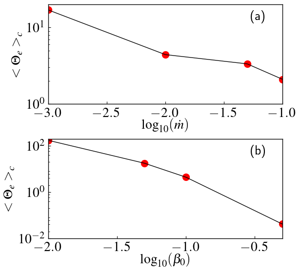
Figure 16: Average coronal temperature is shown as a function of (a) input accretion rate $(\dot{m})$ and the (b) input magnetic field strength ($\beta_{0}$).

The GRRT code BHOSS is currently not equipped to handle the Compton process, therefore in this work, we calculate the average electron temperature of the corona region $(<\Theta_{e}>_{c})$ following,

$$<\Theta_{e}>_{c}=\frac{\sum_{k}\rho^{k}\Theta_{e}^{k}}{\sum_{k}\rho^{k}},$$ (21)

where the summation $(k)$ is carried over all the simulation grids with $-hu_{t}>1$. The Compton efficiency is directly related to the coronal temperature. The higher value of coronal temperature results in a stronger Compton hump and lower corona temperature results in a weaker Compton hump in the emission spectra (e.g., Titarchuk, 1994; Vurm & Poutanen, 2009; Zdziarski et al., 2020, etc.). The plots for time-averaged value $<\Theta_{e}>_{c}$ for different values of accretion rates ($\dot{m}$) and input plasma-$\beta$ ($\beta_{0}$) are shown in Fig. 16. The figures essentially suggest that with the increase in accretion rate, the coronal temperature decreases due to an increase in cooling efficiency. The value of $<\Theta_{e}>_{c}$ drops from $16.93$ to $2.1$ when the accretion rate is increased from $\dot{m}=0.001$ to $\dot{m}=0.1$. On the other hand, with the decrease of magnetic field strength (increase in $\beta_{0}$), the average value of $<\Theta_{e}>_{c}$ decreases due to the reduction of magnetic heating in the flow. The value of $<\Theta_{e}>_{c}$ drops from $173.1$ to $0.042$ when $\beta_{0}$ is decreased from $\beta_{0}=0.1$ to $\beta_{0}=0.5$.

In summary, we found that both parameters $\dot{m}$ and $\beta_{0}$ impact the radiative properties of the thin-disc significantly. From the above discussion, it is evident that an accretion disc with a higher accretion rate and lower magnetic field strength corresponds to a soft spectral state with dominating spectral energy $E>10$keV. With the decrease in accretion rate or the increase in the magnetic field strength, the coronal temperature increases resulting in a soft-intermediate to hard-intermediate spectral state depending on the accretion rate and magnetic field strength.

8 Conclusions and discussion

In this work, we have investigated radiatively cooled thin accretion discs around black holes in the presence of turbulent heating, Coulomb interaction, Bremsstrahlung, synchrotron, Comptonisation of synchrotron photons, and black body radiation. With this, we examined the role of accretion rate and magnetic field strength on the dynamics as well as the radiative properties of the accretion flow. We also studied the properties of the disc-winds with radiative cooling. Below, we summarised our concluding remarks pointwise.

• We find that all of our simulation models remain in SANE accretion flow limit except for the very strong magnetic field case (model G), which becomes MAD with temporal evolution. The SANE models with different input accretion rates show different accretion rates through the event horizon. However, they show similar magnetic flux accumulations around the black hole. On the contrary, the magnetic flux accumulated around the black hole is different for the SANE models with different magnetic field strengths although the accretion rate through the event horizon is similar.

• The input accretion rate and the magnetic field strength both play crucial roles in deciding the properties of the accretion flow. For a higher accretion rate, the electrons are cooler throughout the domain. In comparison with the low accretion rate case, the electrons in the equatorial plane also become cooler for the high accretion rate case. With the increase of the magnetic field strength, the matter in the thin disc puffed up. However, in the case of a very strong magnetic field, the matter in the thin disc is evaporated faster due to the onset of strong disc winds. Also, with the increase of the magnetic field strength, the electrons in the accretion flow become hotter, particularly in the corona region.

• We observe the presence of the $\beta\ll 1$ region above the disc surface, where the ratio $T_{e}/T_{i}\gg 1$ . As a result, the usual $R-\beta$ prescription for describing electron temperature in terms of flow/ion temperature (e.g. Mościbrodzka et al. (2016); Dihingia et al. (2023)) can not provide the trend of electron temperature in the case of a thin disc. Such descriptions are useful only for geometrically thick accretion flow cases (e.g., see Dihingia et al. (2023)).

• We find the ratio of temperatures $T_{e}/T_{i}$ significantly depends on the electrons heating prescriptions. For turbulent heating, the electrons in the funnel region are much hotter compared to the ions. However, in the case of reconnection heating, the electrons in the funnel region mostly remain cooler than the ions.

• We find ample evidence for the active BP disc wind from the thin disc surface. The active area of BP disc wind increases with the increase of input accretion rate as well as the magnetic field strength. The mass flux rate due to the BP disc wind also increases with the input accretion rate and the magnetic field strength.

• By studying the light curves coming from the accretion flow for different input accretion rates and magnetic field strengths, we found that the intensity of the light curves increases both with the accretion rate as well as the magnetic field strength. The light curves at the higher frequencies show much more variable features as compared to the light curves at lower frequencies. In the case of Bremsstrahlung dominated over synchrotron (high frequency, low accretion rate, low magnetic field strength), the light curves do not show variability features.

• The time-averaged spectra also show the importance of the accretion rate and the magnetic field strength in deciding the radiative properties of the accretion flow. The area under the spectra, or the total luminosity, increases with both the accretion rate as well as the magnetic field strength. For higher accretion rates and lower magnetic field cases, the black body component dominates the peak of the emission spectra. For lower accretion rates and higher magnetic field cases, the synchrotron dominates the peak of the emission spectra.

• To understand the contribution of the inverse-Compton process in the emission spectra, we calculate the average coronal temperature $(<\Theta_{e}>_{c})$. We find that $<\Theta_{e}>_{c}$ is anti-correlated with the accretion rate, whereas it is correlated with the strength of the magnetic field.

Based on our study, we find that the accretion rate and the magnetic field strength both play a vital role in deciding the spectral states of an accretion flow. We summarise our understanding of accretion flow in terms of accretion rate limits, magnetic field strength limits, possible spectral states, and characteristics of the outflow in table 2. The table shows a possible link between the accretion rates and the magnetic field strength with the disc winds. Many studies have speculated such bell-shaped behaviour of the accretion rate profile during an outburst (e.g., Esin et al., 1997; Ferreira et al., 2006; Kylafis & Belloni, 2015; Kumar & Yuan, 2022). Also, observations of MAXI J1820+070 show polarised emission in the rising hard state, whereas they show unpolarised emission during the soft and decaying hard state. These facts hint that magnetic field configuration is possibly structured and strong during the rising phase, and the same is weak and unstructured in the decaying phase. Such observations can be can only be comprehended if the magnetic field contribution varies over the timeline of the outburst.

Accretion rate	Field Strenght	States	Disc-winds
Low ($\lesssim 0.01\dot{M}_{\rm Edd}$)	High	High Hard	Structured (BP)
High ($\gtrsim\dot{M}_{\rm Edd}$)	Low	Soft	Turbulent $(B_{\rm tor})$
Low ($\lesssim 0.01\dot{M}_{\rm Edd}$)	Very low	Low Hard	Turbulent $(B_{\rm tor})$

Table 2: Summary of parameters ranges and corresponding spectral states and disc-wind characteristics.

Data Availability

The data underlying this article will be shared on reasonable request to the corresponding author.

References

- Belloni & Motta (2016) Belloni T. M., Motta S. E., 2016, Transient Black Hole Binaries. Springer Berlin, Heidelberg, p. 61, doi:10.1007/978-3-662-52859-4_2
- Belloni et al. (2011) Belloni T. M., Motta S. E., Muñoz-Darias T., 2011, Bulletin of the Astronomical Society of India, 39, 409
- Blandford & Payne (1982) Blandford R. D., Payne D. G., 1982, MNRAS, 199, 883
- Bourouaine et al. (2013) Bourouaine S., Verscharen D., Chandran B. D. G., Maruca B. A., Kasper J. C., 2013, ApJ, 777, L3
- Chael et al. (2018) Chael A., Rowan M., Narayan R., Johnson M., Sironi L., 2018, MNRAS, 478, 5209
- Colpi et al. (1984) Colpi M., Maraschi L., Treves A., 1984, ApJ, 280, 319
- Del Zanna et al. (2007) Del Zanna L., Zanotti O., Bucciantini N., Londrillo P., 2007, A&A, 473, 11
- Dexter et al. (2021) Dexter J., Scepi N., Begelman M. C., 2021, ApJ, 919, L20
- Díaz Trigo & Boirin (2016) Díaz Trigo M., Boirin L., 2016, Astronomische Nachrichten, 337, 368
- Dihingia & Vaidya (2022) Dihingia I. K., Vaidya B., 2022, Journal of Astrophysics and Astronomy, 43, 23
- Dihingia et al. (2018) Dihingia I. K., Das S., Mandal S., 2018, MNRAS, 475, 2164
- Dihingia et al. (2020) Dihingia I. K., Das S., Prabhakar G., Mand al S., 2020, MNRAS, 496, 3043
- Dihingia et al. (2021) Dihingia I. K., Vaidya B., Fendt C., 2021, MNRAS, 505, 3596
- Dihingia et al. (2022) Dihingia I. K., Vaidya B., Fendt C., 2022, MNRAS, 517, 5032
- Dihingia et al. (2023) Dihingia I. K., Mizuno Y., Fromm C. M., Rezzolla L., 2023, MNRAS, 518, 405
- Esin et al. (1996) Esin A. A., Narayan R., Ostriker E., Yi I., 1996, ApJ, 465, 312
- Esin et al. (1997) Esin A. A., McClintock J. E., Narayan R., 1997, ApJ, 489, 865
- Ferreira et al. (2006) Ferreira J., Petrucci P. O., Henri G., Saugé L., Pelletier G., 2006, A&A, 447, 813
- Fragile & Meier (2009) Fragile P. C., Meier D. L., 2009, ApJ, 693, 771
- Gallo et al. (2005) Gallo E., Fender R., Kaiser C., 2005, in Burderi L., Antonelli L. A., D’Antona F., di Salvo T., Israel G. L., Piersanti L., Tornambè A., Straniero O., eds, American Institute of Physics Conference Series Vol. 797, Interacting Binaries: Accretion, Evolution, and Outcomes. pp 189–196 (arXiv:astro-ph/0501374), doi:10.1063/1.2130232
- Howes (2010) Howes G. G., 2010, MNRAS, 409, L104
- Howes (2011) Howes G. G., 2011, ApJ, 738, 40
- Ingram & Motta (2019) Ingram A. R., Motta S. E., 2019, New Astron. Rev., 85, 101524
- Kosenkov et al. (2020) Kosenkov I. A., et al., 2020, MNRAS, 496, L96
- Kumar & Yuan (2022) Kumar R., Yuan Y.-F., 2022, arXiv e-prints, p. arXiv:2210.00683
- Kylafis & Belloni (2015) Kylafis N. D., Belloni T. M., 2015, A&A, 574, A133
- Leung et al. (2011) Leung P. K., Gammie C. F., Noble S. C., 2011, ApJ, 737, 21
- Manmoto et al. (1997) Manmoto T., Mineshige S., Kusunose M., 1997, ApJ, 489, 791
- Mata Sánchez et al. (2022) Mata Sánchez D., et al., 2022, ApJ, 926, L10
- Meringolo et al. (2023) Meringolo C., Cruz-Osorio A., Rezzolla L., Servidio S., 2023, arXiv e-prints, p. arXiv:2301.02669
- Miller et al. (2006) Miller J. M., et al., 2006, ApJ, 646, 394
- Mościbrodzka et al. (2016) Mościbrodzka M., Falcke H., Shiokawa H., 2016, A&A, 586, A38
- Muñoz-Darias et al. (2019) Muñoz-Darias T., et al., 2019, ApJ, 879, L4
- Nakamura et al. (1996) Nakamura K. E., Matsumoto R., Kusunose M., Kato S., 1996, PASJ, 48, 761
- Narayan & Yi (1995) Narayan R., Yi I., 1995, ApJ, 452, 710
- Narayan et al. (1998) Narayan R., Mahadevan R., Grindlay J. E., Popham R. G., Gammie C., 1998, ApJ, 492, 554
- Neilsen (2013) Neilsen J., 2013, Advances in Space Research, 52, 732
- Novikov & Thorne (1973) Novikov I. D., Thorne K. S., 1973, in Black Holes (Les Astres Occlus). pp 343–450
- Page & Thorne (1974) Page D. N., Thorne K. S., 1974, ApJ, 191, 499
- Peitz & Appl (1997) Peitz J., Appl S., 1997, Mon. Not. Roy. Astron. Soc., 286, 681
- Ponti et al. (2012) Ponti G., Fender R. P., Begelman M. C., Dunn R. J. H., Neilsen J., Coriat M., 2012, MNRAS, 422, L11
- Porth et al. (2017) Porth O., Olivares H., Mizuno Y., Younsi Z., Rezzolla L., Moscibrodzka M., Falcke H., Kramer M., 2017, Computational Astrophysics and Cosmology, 4, 1
- Poutanen et al. (2018) Poutanen J., Veledina A., Zdziarski A. A., 2018, A&A, 614, A79
- Ressler et al. (2015) Ressler S. M., Tchekhovskoy A., Quataert E., Chandra M., Gammie C. F., 2015, MNRAS, 454, 1848
- Rezzolla & Zanotti (2013) Rezzolla L., Zanotti O., 2013, Relativistic Hydrodynamics. Oxford University Press
- Riffert & Herold (1995) Riffert H., Herold H., 1995, Astrophys. J., 450, 508
- Rowan et al. (2017) Rowan M. E., Sironi L., Narayan R., 2017, ApJ, 850, 29
- Ryan et al. (2017) Ryan B. R., Ressler S. M., Dolence J. C., Tchekhovskoy A., Gammie C., Quataert E., 2017, ApJ, 844, L24
- Ryan et al. (2018) Ryan B. R., Ressler S. M., Dolence J. C., Gammie C., Quataert E., 2018, ApJ, 864, 126
- Rybicki & Lightman (1979) Rybicki G. B., Lightman A. P., 1979, Radiative processes in astrophysics
- Shiokawa et al. (2012) Shiokawa H., Dolence J. C., Gammie C. F., Noble S. C., 2012, ApJ, 744, 187
- Sądowski et al. (2017) Sądowski A., Wielgus M., Narayan R., Abarca D., McKinney J. C., Chael A., 2017, MNRAS, 466, 705
- Spitzer (1965) Spitzer L., 1965, Physics of fully ionized gases. Dover Publications Inc.
- Steiner et al. (2009) Steiner J. F., Narayan R., McClintock J. E., Ebisawa K., 2009, PASP, 121, 1279
- Tchekhovskoy et al. (2011) Tchekhovskoy A., Narayan R., McKinney J. C., 2011, MNRAS, 418, L79
- Tetarenko et al. (2018) Tetarenko B. E., Lasota J. P., Heinke C. O., Dubus G., Sivakoff G. R., 2018, Nature, 554, 69
- Titarchuk (1994) Titarchuk L., 1994, ApJ, 434, 570
- Titarchuk et al. (2014) Titarchuk L., Seifina E., Shrader C., 2014, ApJ, 789, 98
- Vourellis & Fendt (2021) Vourellis C., Fendt C., 2021, ApJ, 911, 85
- Vourellis et al. (2019) Vourellis C., Fendt C., Qian Q., Noble S. C., 2019, ApJ, 882, 2
- Vurm & Poutanen (2009) Vurm I., Poutanen J., 2009, ApJ, 698, 293
- Wielgus et al. (2022) Wielgus M., et al., 2022, A&A, 665, L6
- Younsi et al. (2012) Younsi Z., Wu K., Fuerst S. V., 2012, A&A, 545, A13
- Younsi et al. (2020) Younsi Z., Porth O., Mizuno Y., Fromm C. M., Olivares H., 2020, in Asada K., de Gouveia Dal Pino E., Giroletti M., Nagai H., Nemmen R., eds, Vol. 342, Perseus in Sicily: From Black Hole to Cluster Outskirts. pp 9–12 (arXiv:1907.09196), doi:10.1017/S1743921318007263
- Younsi et al. (2023) Younsi Z., Psaltis D., Özel F., 2023, ApJ, 942, 47
- Yuan & Narayan (2014) Yuan F., Narayan R., 2014, ARA&A, 52, 529
- Zanni et al. (2007) Zanni C., Ferrari A., Rosner R., Bodo G., Massaglia S., 2007, A&A, 469, 811
- Zdziarski et al. (2020) Zdziarski A. A., Szanecki M., Poutanen J., Gierliński M., Biernacki P., 2020, MNRAS, 492, 5234