Generative Table Pre-training Empowers Models for Tabular Prediction

Abstract

Recently, the topic of table pre-training has attracted considerable research interest. However, how to employ table pre-training to boost the performance of tabular prediction remains an open challenge. In this paper, we propose TaPTaP, the first attempt that leverages table pre-training to empower models for tabular prediction. After pre-training on a large corpus of real-world tabular data, TaPTaP can generate high-quality synthetic tables to support various applications on tabular data, including privacy protection, low resource regime, missing value imputation, and imbalanced classification. Extensive experiments on $12$ datasets demonstrate that TaPTaP outperforms a total of $16$ baselines in different scenarios. Meanwhile, it can be easily combined with various backbone models, including LightGBM, Multilayer Perceptron (MLP) and Transformer. Moreover, with the aid of table pre-training, models trained using synthetic data generated by TaPTaP can even compete with models using the original dataset on half of the experimental datasets, marking a milestone in the development of synthetic tabular data generation. The codes are available at https://github.com/ZhangTP1996/TapTap.

1 Introduction

Recently, pre-trained language models (LMs) have attracted a lot of research interest in different domains, especially in the area of natural language processing. After pre-training on a large-scale unstructured text corpus with a self-supervised training objective, e.g., masked language modeling (MLM) proposed by BERT (Devlin et al., 2019), LMs can significantly benefit downstream tasks. Furthermore, recent progress on generative LMs (Radford et al., 2019; Raffel et al., 2020; Lewis et al., 2020) suggests that it is possible to unify different tasks via one LM. The remarkable success of pre-trained LMs has inspired much research in pre-training over structured tables, one of the most common types of data used in real-world applications (Benjelloun et al., 2020). Different from text, tables usually contain rich and meaningful structural information, and thus LMs on text corpus are not well suited for tabular data. To this end, there has been a growing amount of recent work on table pre-training (Herzig et al., 2020; Yin et al., 2020; Wang et al., 2021b; Liu et al., 2022).

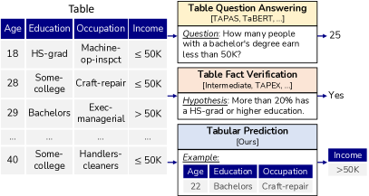
Figure 1: An illustration of different table-related tasks with representative table pre-training models, including TaPaS (Herzig et al., 2020), TaBERT (Yin et al., 2020), Intermediate (Eisenschlos et al., 2020), TaPEx (Liu et al., 2022) and our TaPTaP.

However, the vast majority of existing table pre-training works aim to enhance joint reasoning over text and table (e.g., table question answering, tableQA), while neglecting tabular prediction, an important task in real-world applications. The goal of tabular prediction is to predict a specified target (e.g., the income) based on a set of features (e.g., the age and the occupation). As illustrated in Figure 1, most pre-trained LMs on tables such as TaPaS (Herzig et al., 2020) typically apply MLM variants on crawled tables and text segments to boost their joint reasoning capability in tableQA.

Nevertheless, as of yet, there is little evidence that these table pre-training methods can enhance the performance of tabular prediction tasks. This is probably because tabular prediction tasks are quite challenging. In contrast to the exceptional performance of deep learning in many domains, recent studies (Shwartz-Ziv and Armon, 2022; Gorishniy et al., 2021) question the necessity of deep learning models for tabular prediction, as their performance is usually outperformed by traditional machine learning models. To summarize, it is still an open challenge to employ table pre-training to boost models for the tabular prediction task.

In this paper, we present TaPTaP (Table Pre-training for Tabular Prediction), which is the first attempt that leverages table pre-training to benefit tabular prediction tasks significantly. To benefit different backbone models, we apply table pre-training from a data perspective, i.e., we utilize TaPTaP to synthesize high-quality examples that can be used to train backbone models. Based on the widely used generative language model GPT (Radford et al., 2019), after ongoing pre-training on a large-scale corpus of real-world tabular data, TaPTaP is expected to capture a generic tabular data distribution. Then, TaPTaP can be quickly adapted to downstream tables via fine-tuning and can generate high-quality synthetic tables to support various applications on tabular data, including privacy protection, low resource regime, missing value imputation, and imbalanced classification. Meanwhile, such a design decouples the backbone model from the pre-trained model architecture, allowing TaPTaP to benefit different backbone models. Extensive experiments on $12$ public datasets demonstrate that generative table pre-training can empower models on tabular prediction in various ways, and TaPTaP outperforms a total of $16$ baselines in different scenarios and supports three state-of-the-art (SOTA) backbone models. The contributions of this paper can be summarized as follows:

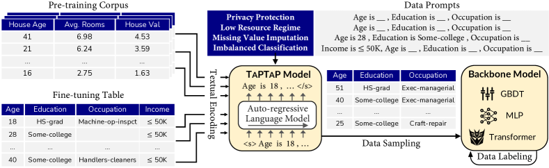
Figure 2: The illustration of our method. The TaPTaP model is firstly pre-trained on the pre-training corpus, and then fine-tuned on the downstream table. During both pre-training and fine-tuning, tables are serialized into sequences via textual encoding, and TaPTaP is trained to predict them token by token. During inference, TaPTaP is prompted to sample values for “   ” in data prompts, and the filled values build up a synthetic table. Finally, once the backbone model has yielded labels for the synthetic table, it can be used to strengthen the backbone model.

• To our knowledge, we are the first to successfully apply table pre-training to tabular prediction. With carefully designed generation strategies, our method combines the advantages of backbone models for tabular prediction and pre-trained LMs.

• To accomplish the pre-training, we collect and filter out $450$ public tabular datasets from Kaggle, UCI, and OpenML platforms, and finally construct a large-scale pre-training corpus.

• To systematically evaluate the proposed table pre-training method, we build a comprehensive benchmark covering four practical settings in tabular prediction. Experimental results on the benchmark demonstrate that TaPTaP can be easily combined with different SOTA backbone models and outperforms a total of $16$ baselines across $12$ datasets.

2 Related Work

Table Pre-training

Previous works on table pre-training can be categorized by the applicable downstream tasks and can be divided into four lines (Dong et al., 2022): table question answering which outputs the answer for questions over tables (Yin et al., 2020; Herzig et al., 2020; Yu et al., 2021; Liu et al., 2022; Andrejczuk et al., 2022), table fact verification which verifies whether a hypothesis holds based on the given table (Eisenschlos et al., 2020), table to text which generates textual descriptions from the given table (Gong et al., 2020; Xing and Wan, 2021) and table structure understanding which aims at identifying structural types in the given table (Tang et al., 2021; Wang et al., 2021b; Deng et al., 2021). Our work is different from theirs because we focus on the application of table pre-training on tabular prediction, an important yet challenging task in real life applications.

Table Generation

TaPTaP supports backbone models by generating synthetic tables, and thus it is close to the line of table generation. Existing methods for the generation of synthetic tabular data mostly leverage generative adversarial networks (Choi et al., 2017; Park et al., 2018; Mottini et al., 2018; Xu et al., 2019; Koivu et al., 2020) or variational autoencoders (Xu et al., 2019; Ma et al., 2020; Darabi and Elor, 2021). However, it is hard for these methods to leverage the textual semantics in tables. More recently, GReaT (Borisov et al., 2022) has successfully applied LMs in generating synthetic tabular data, which inspired us a lot. However, GReaT only exploits existing LMs for privacy protection, while our proposed table pre-training can significantly improve models for tabular prediction in various scenarios.

Tabular Prediction

Due to the tremendous success of deep learning and transfer learning in various domains, there has been a lot of research interest to extend this success to tabular prediction (Song et al., 2019; Wang et al., 2021a; Arik and Pfister, 2021). As for deep learning, we refer readers to Gorishniy et al. (2021) for a comprehensive comparison of different deep learning models for tabular data. Our work is technically orthogonal to these efforts, as it can be integrated with different backbone models (e.g., Transformer). As for transfer learning, there has been some pioneering attempts (Levin et al., 2022; Wang and Sun, 2022). More recently, researchers even explore the ability of LMs on zero / few-shot classification of tabular data (Hegselmann et al., 2022). However, there is often some gap between their experimental setup and real-world applications. For example, Levin et al. (2022) only investigates transfer learning on tables with lots of overlapping columns. In contrast, our method can generally adapt well to different tables after once pre-training. Despite all these efforts in advancing deep learning on tabular data, recent studies (Shwartz-Ziv and Armon, 2022; Gorishniy et al., 2021; Grinsztajn et al., 2022) found that machine learning models like XGBoost (Chen and Guestrin, 2016) and LightGBM (Ke et al., 2017) still outperformed those deep-learning counterparts. To this end, TaPTaP aims at synthesizing high-quality examples, which is able to empower both machine learning and deep learning models.

3 Methodology

In this section, we first formally introduce the tabular prediction task and then present our approach.

3.1 Preliminary of Tabular Prediction

A tabular data usually contains two parts, the features and the label. Given the features as the input, the goal of tabular prediction is to predict the label. Taking the example from Figure 1, the task is to predict the income (label) of a person based on her / his age, education and occupation (features). Below we formalize tabular prediction using the binary-classification task, and the formulation can be easily extended to multi-class classification or regression problems. Formally, a tabular data with $n$ samples (i.e., rows) and $m$ features (i.e., columes) can be represented by $D\!=\!\!\{(\mathbf{x}_{i},y_{i})\}_{i=1,\ldots,n}$ where $\mathbf{x}_{i}\!\!=\!\!(x_{i,1},\cdots,x_{i,j},\cdots,x_{i,m})\in\mathbb{R}^{m}$ and $y_{i}\in\{0,1\}$. The $j$-th feature has a feature name $f_{j}$ (e.g., “age”). A model $F$ takes the features $\mathbf{x}_{i}$ as input to predict the label $y_{i}$. Our goal is to train a model such that the test error is as small as possible.

Existing works on improving $F$ either design better model architectures Gorishniy et al. (2021) or improve the quality of training data (Zhang et al., 2022). We follow the second path to improve the model performance by generating synthetic data, since many challenges in tabular prediction are due to the expensive nature of the data collection process and can be tackled with data generation.

There are four typical scenarios where high-quality synthetic samples are helpful: (1) Privacy protection (Gascón et al., 2017). In many application domains, each party only has part of the dataset and several parties can collaboratively train a model on a joint dataset. But tabular data usually contains sensitive personal information or confidential business secrets that cannot be directly shared with other parties. In this case, TaPTaP can be used to generate synthetic data $D_{s}$ to replace the real data $D$, while achieving similar model performance. (2) Low resource regime. Data collection can be very expensive in some applications and hence handling the small data regime is an important challenge. For example, over $44$% classification datasets on the UCI platform (Asuncion and Newman, 2007) have less than $1000$ samples. In this case, we can leverage TaPTaP to perform data augmentation in order to boost the backbone model. (3) Missing value imputation. Missing values are ubiquitous in tabular data (Stekhoven and Bühlmann, 2012). In this case, TaPTaP is able to impute the missing values to improve the performance of the model. (4) Imbalanced classification. It is common to have a long-tail label distribution in tabular data (Cao et al., 2019). In this case, TaPTaP can be used to balance the class distribution by conditional sampling (from the minority classes).

3.2 Overview

As shown in Figure 2, TaPTaP consists of four steps. (1) Pre-training: train an auto-regressive LM on the table pre-training corpus compiled by lots of public tabular datasets. (2) Fine-tuning: train the LM on the downstream table; (3) Data Sampling: prompt the fine-tuned LM to sample synthetic tables with only tabular features. (4) Data Labeling: assign pseudo labels to the synthetic tables via downstream backbone models. Below we describe these steps in details.

3.3 Pre-training

Corpus Construction

To build the pre-training corpus, we leverage publicly available tabular datasets from Kaggle, UCI Asuncion and Newman (2007), and OpenML Vanschoren et al. (2013) platforms. We believe the table pre-training should be performed on tabular data with rich semantic information, therefore we eliminate datasets with meaningless column names (e.g., V1). After the filtering, we finally collect $450$ tabular datasets with a total of nearly $2$ million samples. To illustrate it better, we show in Figure 3 a word cloud composed of feature names and feature values. Note that we are careful to guarantee that the tabular datasets used in pre-training and the downstream benchmark datasets are non-overlapping, so there is no data leakage issue.

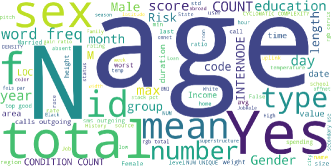
Figure 3: The word cloud for the pre-training corpus.

3.3.1 Textual Encoding

Table Serialization

Since TaPTaP starts with the GPT model, we follow the previous work (Borisov et al., 2022; Liu et al., 2022) to serialize each sample into a sequence of tokens to reduce the difficulty of table pre-training. As suggested by Hegselmann et al. (2022), we take the text template serialization strategy and serialize samples using the “[Feature] is [Value]” template. Taking the example in Figure 2, the first sample in the fine-tuning table is converted into a sentence “Age is 18, Education is HS-grad, Occupation is Machine-op-inspct, Income is $\leq$ 50K”. Formally, given a table $D=\{(\mathbf{x}_{i},y_{i})\}$, let $x_{i,j}$ be the $j$-th feature value in $\mathbf{x}_{i}$ and $f_{j}$ be the $j$-th feature name. The textual encoding is to transform the $i$-th sample $\mathbf{x}_{i}$ into a splice of sentences separated by commas $\mathbf{t}_{i}=(t_{i,1},\text{``,''},t_{i,2},\cdots,\text{``,''},t_{i,m})$, where $t_{i,j}=(f_{j},\text{``is''},x_{i,j})$.

Number Encoding

Numerical features (e.g., age) are important and widely used in tabular data - over $70$% of features in our pre-training corpus are numerical features, but how to properly encode these features has always been neglected in previous work of tabular prediction. Meanwhile, recent studies on LMs show that they are not good at dealing with numbers (Pi et al., 2022) and suggest the character-level representation is better suited to capture the number semantics than its counterparts (Wallace et al., 2019). Therefore, we use the character-level representation for all numerical features, which means that the phrase “Age is 18” in Figure 2 would be converted into “Age is 1 8”.

Table 1: Properties of benchmark datasets.

Dataset	Classification							Regression
	LO	AD	HE	CR	SI	BE	DI	CA	GE	ME	AG	DU
# samples (k)	0.6	49	9.9	150	3.8	14	102	21	27	1.3	3.9	1.9
# numerical features	5	6	23	10	6	16	8	8	6	3	7	34
# categorical features	6	8	0	0	22	0	39	0	3	3	1	2
# classes	2	2	2	2	2	7	3	-	-	-	-	-

Permutation Function

The features in the tabular data are not ordered, but they are encoded as an ordered sentence, which introduces spurious positional relationships in textual encoding. In order to reconstruct the order independence among features, we follow previous work Borisov et al. (2022) to apply a permutation function $\mathcal{P}$ to randomly shuffle the order of features when encoding a table. Therefore, the encoded sentence becomes $\mathbf{t}_{i}=(t_{i,k_{1}},\text{``,''},t_{i,k_{2}},\cdots,\text{``,''},t_{i,k_{m}})$, where $[k_{1},k_{2},\cdots,k_{m}]=\mathcal{P}([1,2,\cdots,m])$. As indicated by Borisov et al. (2022), such permutation enables conditional sampling when doing inference on downstream tables, i.e., TaPTaP can generate a synthetic sample conditioned on any set of known features. We take a step further to demonstrate that the conditional sampling helps TaPTaP perform well in the missing value imputation scenario.

3.3.2 Pre-training Procedure

As mentioned before, the pre-training follows an auto-regressive manner, i.e., TaPTaP is trained to predict the encoded sentence token by token. Assuming we have $q$ tabular datasets for pre-training, the whole pre-training corpus $\mathcal{T}$ can be obtained by combining each tabular data after textual encoding as $\{\mathbf{t}_{i}^{(1)}\cup\cdots\cup\mathbf{t}_{i}^{(q)}\}$. Then, each sentence $\mathbf{t}\in\mathcal{T}$ can be encoded into a sequence of tokens using $(w_{1},\cdots,w_{N})=\mathtt{tokenize}(\mathbf{t})$. In general, TaPTaP factorizes the probability of generating $\mathbf{t}$ in an auto-regressive manner as $p(\mathbf{t})=\prod_{k=1}^{N}p(w_{k}|w_{1},\cdots,w_{k-1})$. During pre-training, TaPTaP is optimized towards maximizing the probability $\prod_{i=1}^{|\mathcal{T}|}p(\mathbf{t}_{i})$ on the entire pre-training corpus. The pre-training can start with any auto-regressive LM such as GPT Radford et al. (2019), so that TaPTaP can benefit from the common knowledge already learned by these LMs.

3.4 Fine-tuning

Fine-tuning TaPTaP on the downstream table follows a similar procedure as in pre-training. The only difference is that the encoded sentences for fine-tuning are generated by applying textual encoding to the downstream table.

3.5 Data Sampling

Given the sequence $(w_{1},\cdots,w_{k-1})$ as the prompt, TaPTaP is able to output the categorical distribution of the next token $w_{k}\in\mathcal{V}$ after fine-tuning, where $\mathcal{V}$ denotes the vocabulary. In general, $w_{k}$ is sampled from the conditioned probability distribution $p(w_{k}|w_{1},\cdots,w_{k-1})$.

Since we also employ permutation during fine-tuning, the fine-tuned TaPTaP is able to generate synthetic samples given any prompt. Similar to Borisov et al. (2022), we employ three kinds of prompting strategies for different application scenarios. (1) Feature name as prompt. This strategy is used in the privacy protection and low resource regime, where only feature names in the tabular data are selected as the prompt. The synthetic samples are generated by TaPTaP according to the prompt “[Feature] is ”. (2) One feature-value pair as prompt. This strategy is used in the imbalanced classification scenario, where the feature names and the minority label(s) are both provided as the prompt. With the label treated as a feature, TaPTaP generates synthetic samples based on the prompt “[Feature] is [Value], ”. (3) Multiple feature-value pairs as prompt. This strategy is used in the missing feature scenarios, where the feature names and available feature values are provided as the prompt. TaPTaP generates synthetic samples according to the prompt “[Feature1] is [Value1], [Feature2] is [Value2], $\cdots$, ”. The order of the given features in the prompt is random. Data prompt examples can be found in Figure 2.

Table 2: The experimental results in privacy protection. Here we present the difference in metrics between the model trained on the synthetic data and the one trained on the original data, the lower the better. A gap close to zero suggests that the synthetic data is of comparable quality to the original data. Below the backbone model is LightGBM. Results of MLP and Transformer can be found in Table 13 and 14.

Diff. w.r.t. Origin $\downarrow$	LO	AD	HE	CR	SI	BE	DI	CA	GE	ME	AG	DU	Avg. Rank
CTGAN	12.1	3.7	8.6	87.2	4	24.2	5.6	38.4	14.3	101.1	27.5	104.1	5.88 $\pm$ 0.91
CopulaGAN	14.2	3.4	8.7	0.2	4	27.8	5.5	57.3	14.5	83.6	26.6	105.7	5.79 $\pm$ 1.47
TVAE	14	5.7	0.8	1.4	7.6	7.9	2.6	16.7	5.1	109.4	33.7	34.2	5.00 $\pm$ 1.41
GReaT-distill	1.4	2	2.8	2.4	19.8	1.8	4.8	22.8	8.1	8.4	7.6	87.7	4.50 $\pm$ 1.09
GReaT	2.5	0.9	3.7	2.6	14.5	1.9	1.7	13.1	2.4	0.7	4.5	25.7	3.75 $\pm$ 1.29
TaPTaP-distill	0	0.7	0.4	0	1.1	0.4	1.6	3.7	0.7	0.2	0.6	16.7	1.71 $\pm$ 0.45
TaPTaP	0	0.5	0.3	0	0.6	0.4	1.6	2.5	1.5	0	4.6	12.8	1.38 $\pm$ 0.64

Table 3: The experimental results in low resource regime. “+ Ori” means training with the original data. “+ Ori + Synthetic Data” means training with the original data plus the synthetic data. Below the backbone model is Transformer with piece-wise linear encoding. The full results on all datasets can be found in Table 15 and 16.

Metric $\uparrow$	LO	HE	BE	SI	CA	GE	ME	AG	DU	Avg. Rank
Transformer + Ori	76.8	72.5	92.7	98.5	82.9	98.2	86.6	52.6	96.5	-
Transformer + Ori + Synthetic Data by Models
CTGAN	74.7	71.5	92.7	97.8	81.5	96.3	72.1	51.6	71.7	5.83 $\pm$ 1.27
CopulaGAN	74.7	71.8	92.5	97.8	81.7	95.9	72.8	52.0	86.8	5.39 $\pm$ 1.32
TVAE	76.2	72.8	92.5	97.4	82.0	97.2	85.7	47.3	80.0	4.56 $\pm$ 2.01
GReaT-distill	76.1	72.0	92.6	98.3	77.9	96.6	86.2	52.4	79.0	4.89 $\pm$ 1.05
GReaT	74.5	72.1	92.7	98.4	80.5	98.1	86.4	53.3	80.3	4.11 $\pm$ 1.45
TaPTaP-distill	76.2	72.5	92.8	98.5	83.7	98.2	86.9	53.8	98.2	1.78 $\pm$ 0.67
TaPTaP	77.5	72.5	92.9	98.5	83.7	98.2	86.7	53.5	97.9	1.44 $\pm$ 0.53

3.6 Data Labeling

An accurate label is arguably one of the most crucial ingredients in synthetic samples. Noisy labels can severely degrade the generalization capability of backbone models (Gorishniy et al., 2021). In contrast to the previous work relying on LMs to generate labels (Borisov et al., 2022), we propose to assign pseudo labels using the SOTA backbone models. We argue that LMs are not the best choice for label generation, since most commonly used tabular prediction models (e.g., LightGBM) are carefully designed for tabular data and generally more accurate at predicting the labels (Hegselmann et al., 2022; Shwartz-Ziv and Armon, 2022).

Formally, given a downstream table $D\!\!=\!\!\{(\mathbf{x}_{i},y_{i})\}$, we first fine-tune TaPTaP on it to generate synthetic tabular features $\{\mathbf{x}_{i}^{\prime}\}$. Next, a backbone model $F$ is trained to fit the original table $D$. Then, the synthetic labels $y_{i}^{\prime}$ can be derived using the well-trained model via $y_{i}^{\prime}\!=\!F(\mathbf{x}_{i}^{\prime})$. Finally, the synthetic labels and the synthetic tabular features make up the final synthetic table $D_{s}\!=\!\{(\mathbf{x}_{i}^{\prime},y_{i}^{\prime})\}$. The following model analysis in the Section 4.3 reveals that our design of data labeling (i.e., not using LMs for label generation) is crucial for the superior performance of our approach.

4 Experiments

4.1 Experimental Setup

Datasets and Evaluation Metrics

We collect $12$ diverse real-world datasets from various domains (Asuncion and Newman, 2007; Vanschoren et al., 2013). Each dataset is split into a train set ($75$%) and a test set ($25$%), and all experiments share the same splits. We provide some important statistics of each dataset in Table 1 and more details in Appendix A. Following previous works (Grinsztajn et al., 2022; Borisov et al., 2022), we use accuracy and R2 score as the evaluation metrics for the classification and regression tasks. For the imbalanced classification scenario, we employ AUC as the evaluation metric. All the experimental results are averaged over $10$ different random seeds.

Backbone Models

To comprehensively evaluate TaPTaP, we experiment with various SOTA backbone models for tabular prediction, including LightGBM (Ke et al., 2017), MLP, and Transformer (Gorishniy et al., 2021). Modern GBDT models (such as LightGBM, Xgboost, CatBoost (Prokhorenkova et al., 2018)) have been the most popular models for the tabular prediction area in the past few years (Gorishniy et al., 2021; Shwartz-Ziv and Armon, 2022). We choose LightGBM in our experiments. Recently, MLP and Transformer with piece-wise linear encoding (Gorishniy et al., 2022) are proposed to be competitive neural network alternatives against LightGBM.

Language Models

TaPTaP uses the original GPT2 (Radford et al., 2019) with $355$M parameters, while TaPTaP-distill uses the distilled version of GPT2 (Sanh et al., 2019) with $82$M parameters.

4.2 Main Results

Table 4: The experimental results in missing value imputation. “+ M-Ori” means training with the original data processed by the MCAR mechanism. “+ M-Ori + Synthetic Data” means training with the M-Ori data where the missing values are imputed by different models. Below the backbone model is MLP. Results using LightGBM and Transformer as backbone models can be found in Table 17 and 18. Results with the MAR mechanism can be found in Appendix B.5. ✗ denotes the method cannot run successfully on the dataset due to too many missing values.

Metric $\uparrow$	LO	AD	HE	CR	SI	BE	DI	CA	GE	ME	AG	DU	Avg. Rank
MLP + M-Ori	73.2	85.4	71.1	93.6	95.6	90.3	57.4	63.1	93.0	68.4	41.4	70.6	-
MLP + M-Ori + Synthetic Data by Models
MIWAE	71.3	✗	68.7	✗	95.7	90.0	✗	59.0	90.6	65.0	42.6	75.7	7.54 $\pm$ 0.78
Sinkhorn	73.2	83.9	69.3	93.5	95.8	88.6	56.6	62.5	93.4	73.3	49.9	72.8	5.75 $\pm$ 1.14
GAIN	86.2	86.2	72.9	57.6	97.6	90.9	53.8	54.9	92.9	69.4	44.2	82.0	5.00 $\pm$ 2.49
MICE	73.1	84.5	70.0	93.6	96.0	88.3	57.2	63.0	93.8	72.3	53.1	91.1	4.75 $\pm$ 1.82
MissForest	72.9	79.8	69.9	92.7	96.7	91.6	57.2	74.0	94.2	79.5	46.4	88.5	4.75 $\pm$ 1.54
HyperImpute	73.4	86.7	70.5	83.0	96.8	92.8	✗	77.7	96.2	78.4	58.1	90.6	3.54 $\pm$ 1.78
TaPTaP-distill	74.9	86.9	72.2	93.7	97.5	93.4	57.2	78.5	94.5	72.6	53.6	69.2	2.83 $\pm$ 1.90
TaPTaP	73.6	87.0	73.0	93.7	96.9	93.1	57.8	82.7	97.3	81.2	53.2	85.5	1.83 $\pm$ 1.11

We directly measure the quality of the synthesized samples according to their performance in different application scenarios.

Privacy Protection

Following the previous work (Borisov et al., 2022), we include baselines CT-GAN (Xu et al., 2019), TVAE (Xu et al., 2019), CopulaGAN (Patki et al., 2016), GReaT-distill and GReaT (Borisov et al., 2022). All methods are used to generate the same amount of synthetic data as the original dataset. The backbone models are trained on the synthetic data, and then evaluated on the original test set. The experimental results are presented in Table 2. One can observe that TaPTaP and TaPTaP-distill outperform most of the baseline methods. Noticing that GReaT also utilizes GPT2, the fact that TaPTaP surpasses it by a large margin suggests the superiority of table pre-training. More importantly, with table pre-training, the quality of the synthetic data generated by TaPTaP can even match that of the original data. On half of the privacy protection datasets, LightGBM models trained with our synthetic data achieve almost the same performance as with the original data. This is highly impressive, especially when considering that none of the synthetic samples appear in the original dataset.

Low Resource Regime

We perform data augmentation to mitigate the low resource dilemma. The baseline methods are identical to those in privacy protection. During fine-tuning, following the experience of multi-task learning in T5 (Raffel et al., 2020), we first use the synthetic data to fine-tune a backbone model. Then, we use the original data to continually fine-tune the model. Experimental results on $9$ datasets with less than $30$k samples are presented in Table 3, which show that TaPTaP is able to perform comparably or better than all baseline methods on most datasets. Furthermore, TaPTaP contribute significant gains to $4$ of the $9$ datasets, which is highly non-trivial.

Missing Value Imputation

We compare with top methods as baselines in a recent benchmarking study Jarrett et al. (2022), including GAIN (Yoon et al., 2018), HyperImpute (Jarrett et al., 2022), MICE (Van Buuren and Groothuis-Oudshoorn, 2011), MissForest (Stekhoven and Bühlmann, 2012), MIWAE (Mattei and Frellsen, 2019), and Sinkhorn (Muzellec et al., 2020). Following previous work (Jarrett et al., 2022), two missing mechanisms are used to yield missing values: missing completely at random (MCAR) and missing at random (MAR). The miss ratio is set to be $0.3$. We present the results in Table 4. As observed, TaPTaP always outperforms most baseline methods using one LM and receives the highest average ranking, indicating its superiority.

Table 5: Experimental results in imbalanced classification. “I-Ori” is the imbalanced data. Below the backbone model is LightGBM. ✗  denotes the method cannot run successfully on the dataset due to too few samples in the minority class. The metric is AUC.

Metric $\uparrow$	LO	AD	HE	CR	SI	Avg. Rank
LightGBM + I-Ori	71.2	90.2	82.3	84.0	99.4	-
LightGBM + I-Ori + Synthetic Data by Models
SMOTE+ENN	✗	87.9	77.7	83.7	98.9	7.30 $\pm$ 0.97
SMOTE+Tomek	✗	89.3	80.3	84.1	99.5	5.80 $\pm$ 1.44
ADASYN	✗	89.5	79.6	84.0	99.5	5.30 $\pm$ 0.97
Random	51.7	89.4	82.3	82.9	99.7	5.00 $\pm$ 2.00
SMOTE	✗	89.5	80.3	84.1	99.5	5.00 $\pm$ 1.37
Borderline	71.2	89.6	79.3	83.5	99.8	4.20 $\pm$ 2.68
TaPTaP-distill	73.0	91.3	83.8	84.8	99.7	1.80 $\pm$ 0.45
TaPTaP	85.5	91.3	83.0	85.0	99.7	1.60 $\pm$ 0.89

Imbalanced Classification

By generating synthetic samples for the minority class, TaPTaP addresses the imbalanced classification problem. Therefore, we compare our methods against popular oversampling methods (Camino et al., 2020), including Random, SMOTE (Chawla et al., 2002), ADASYN (He et al., 2008), Borderline (Han et al., 2005), SMOTE+ENN (Alejo et al., 2010) and SMOTE+Tomek (Zeng et al., 2016). Following the standard approach (Buda et al., 2018), we down-sample the minority class of each binary-classification dataset so that the imbalanced ratio is $50$ ($\text{\#majority}\,/\,{\text{\#minority}}\!\!=\!\!50$). Experimental results on five binary-classification datasets are presented in Table 5, where TaPTaP still has the highest average ranking among all baselines.

Overall Summarization

First, TaPTaP generally improves the performance of different backbone models in tabular prediction and outperforms the majority of baseline methods on various tabular prediction scenarios. Second, the advantage of TaPTaP over TaPTaP-distill suggests that table pre-training can also benefit from scaling up LMs. Third, TaPTaP is the first to successfully generate synthetic data for comparable backbone model performance to original data.

4.3 Ablation Study

Figure 4: Experimental results in the ablation study. The y-axis is the average metric values across all datasets in the privacy protection setting with LightGBM.

Figure 5: Sampling diversity in terms of the coverage score averaged across datasets.

To investigate the effectiveness of each component in TaPTaP, we conduct an ablation study. We name TaPTaP without different components as follows: (1) w.o. pre-training refers to TaPTaP without table pre-training. (2) w.o. data labeling refers to TaPTaP using LMs to generate labels. (3) w.o. character refers to TaPTaP without using the character-level representations for numerical features. (4) w.o. feature name. The column names of each dataset are replaced by dummy names (e.g., “V1”) to remove semantic information.

The experimental results are visualized in Figure 4. We present the average metric values (i.e., Acc. or R2) of each method across $12$ datasets in the privacy protection setting, since it is the most straightforward setting to indicate the quality of synthetic data. We can see that pre-training and data labeling are particularly important for TaPTaP. The semantic information in column names and the character-level representation to enhance number encoding also provide considerable improvement.

4.4 Analysis

Figure 6: The influence of pre-training scale on the downstream performance. The value of each method is the average metric values across all datasets in the privacy protection setting with LightGBM.

Sampling Diversity

We employ the coverage score Naeem et al. (2020) to quantitatively evaluate the sampling diversity of TaPTaP and baseline methods. The coverage refers to the proportion of actual records that contain at least one synthetic record within its manifold. A manifold is defined as a sphere surrounding the sample, with a radius of r determined by the distance between the sample and its k-th nearest neighbor. We present the averaged coverage score in Figure 5.

The Scale of Pre-training Corpus

Figure 6 illustrates the influence of the pre-training scale on the downstream performance. We present the results with $0.02$, $0.1$, $0.5$ and $2$ million samples. As one can observe, scaling up the pre-training corpus brings positive effects. However, the number of high-quality real-world tabular datasets is limited. Therefore, it may be helpful to take advantage of the millions of tables available on the Web.

Table 6: The comparison between TaPTaP and TaPTaP with additional web tables for pre-training.

	AD	HE	CR	SI	DI	CA
TaPTaP	87.5	72.2	93.8	97.6	57.8	81.5
+ Web Tables	87.7	72.3	93.8	98.2	57.6	82.1

Pre-training using Web Tables

To explore the above direction, we present a preliminary study on using tables from Web for pre-training. We parse over $130$k Web tables with a total of $8$ million samples from the WikiTables corpus (Bhagavatula et al., 2015). We use the Web tables together with the tabular datasets for pre-training. The results of the privacy protection setting are presented in Table 6. We can see that even with a large number of Web tables, it is still hard to further boost the backbone models. We attribute it to the quality issue. The collected tabular datasets have already been examined by the platforms, and usually have higher quality than noisy Web tables. How to automatically identify high-quality tables from the huge number of Web tables for pre-training is a promising future direction.

5 Conclusion & Future Work

In this paper, we propose TaPTaP, a table pre-training method to empower models for tabular prediction. It can be combined with various backbone models and boost them via synthesizing high-quality tabular data. A large-scale empirical study demonstrates that TaPTaP can benefit different SOTA backbone models on four tabular prediction scenarios. In the future, we plan to extend TaPTaP to process tables with a large number of features.

Limitations

The major limitation of TaPTaP is the scalability. While we enjoy the advantages of LMs, we also introduce the drawbacks of LMs. In practice, TaPTaP usually requires more running time and GPU memory than other methods. Detailed comparison can be found in Appendix B.2. In addition, TaPTaP can only process tabular data with less than $100$ features due to the input length limitation that GPT can process (i.e., $1024$ tokens).

Ethics Statement

In this paper, we collected and filtered out $450$ publicly available tabular datasets to construct the pre-training corpus for TaPTaP. As these datasets have been reviewed by well-known machine learning platforms such as Kaggle, they should have no private information about individuals. However, we cannot confirm whether these datasets contain potential biases since the corpus contains millions of samples. For example, there may be tables that have the potential to wrongly associate recruitment result to gender. Also, since our model is pre-trained based on GPT, readers may be concerned that the synthetic tables generated by our model contain offensive content. On this point, we argue that one might not be worried too much since for categorical features, our model can be easily tuned to only generate the values that appear in the downstream table, which is relatively controllable.

Table 7: The urls of test datasets.

Dataset	Link
Adult Income (AD) (Kohavi, 1996)	https://archive.ics.uci.edu/ml/datasets/Adult
HELOC (HE)	https://www.kaggle.com/datasets/averkiyoliabev/home-equity-line-of-creditheloc
California Housing (CA) (Pace and Barry, 1997)	https://www.kaggle.com/datasets/camnugent/california-housing-prices
Diabetes (DI) (Strack et al., 2014)	https://www.kaggle.com/c/1056lab-diabetes-readmission-prediction
Credit Scoring (CR) (Credit Fusion, 2011)	https://www.kaggle.com/competitions/GiveMeSomeCredit/overview
Loan (LO)	https://www.openml.org/search?type=data&status=active&sort=match&id=43595
Dubai Housing (DU)	https://www.kaggle.com/datasets/dataregress/dubai-properties-dataset
Crab Age (AG) (Sidhu, 2021)	https://www.kaggle.com/datasets/sidhus/crab-age-prediction
Medical Cost (ME)	https://www.kaggle.com/datasets/mirichoi0218/insurance
Gem Price (GE)	https://www.kaggle.com/datasets/colearninglounge/gemstone-price-prediction
Bean Type (BE) (Koklu and Özkan, 2020)	https://archive.ics.uci.edu/ml/datasets/Dry+Bean+Dataset
Sick Record (SI) (Quinlan, 1987)	https://www.openml.org/search?type=data&sort=runs&id=38&status=active

Appendix A Datasets

We provide the urls of the public datasets in Table 7. These datasets are publicly available, and their license permits usage for research purposes.

Appendix B Additional Experiments

B.1 Distance to Closest Record

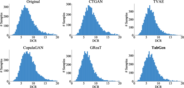
Figure 7: Distance to closest record (DCR) distribution of the California Housing dataset. “Original” denotes the DCR of the original test set with respect to the original train set. The experimental results illustrate that each method does not copy samples from the train set.

In order to demonstrate that TaPTaP generates synthetic samples similar to the original data instead of copying the original data, following the standard approach (Borisov et al., 2022), we calculate each sample’s distance to the closest record (DCR) in the original training data $D$. For each synthetic sample $x$, its DCR is $DCR(s)=min\{Distance(s,s_{i})|s_{i}\in D\}$. We use the $L_{1}$ distance for numerical features. For categorical features, we set the distance to be 0 for equal categories and 1 otherwise. We present the results of California Housing and HELOC in Figure 7 and 8.

B.2 Running Time Comparison

We analyze the running time of TaPTaP, TaPTaP-distill, and baseline methods. The experiments are carried out on a single NVIDIA GeForce RTX 3090 with 24 GB RAM, 64 system RAM, and Intel(R) Xeon(R) Platinum 8350C CPU @ 2.60GHz with 16 cores. For the privacy protection setting, we present the running time of training/fine-tuning and sampling separately. We present the results of the Adult Income dataset in Table 8. For the missing value imputation setting, we present the running time of the California Housing dataset in Table 9. We can see that TaPTaP and TaPTaP-distill requires more running time than most of the baseline methods. While we enjoy the benefits of leveraging LMs to achieve top performance, we also introduce the drawbacks of LMs in requiring more computational resources. However, there are important real-world applications such as healthcare or finance where achieving better performance outweighs saving computational time. In addition, the fine-tuning and sampling time can be reduced by using more computational resources.

B.3 Privacy Protection

Table 2, 13 and 14 show the performance of our method and baseline methods in privacy protection setting with LightGBM, MLP, and Transformer as the backbone.

B.4 Low Resource Regime

Table 15 and 16 show the performance of our method and baseline methods in low resource regime setting with MLP and Transformer as the backbone. Note that both low resource datasets and high resource datasets are presented in the table.

B.5 Missing Value Imputation

Table 17, 4 and 18 show the performance of our method and baseline methods in missing value imputation setting using MCAR mechanism with LightGBM, MLP, and Transformer as the backbone. Table 19, 20 and 21 show the performance of our method and baseline methods in missing value imputation setting using MAR mechanism with LightGBM, MLP, and Transformer as the backbone. MIWAE and HyperImpute fail on some datasets because one feature in the dataset contains too many missing values. For example, 96.9% of data points in the “weight” column in the Diabetes dataset are missing. However, the methods require at least one valid value for each training batch.

B.6 Imbalance Classification

Table 5 shows the performance of our method and baseline methods in the imbalance classification setting with LightGBM as the backbone. Smote-based methods fail on the Loan dataset because there are fewer than 10 minority class data, which results in the number of sampled data points being less than the number of neighbors(Chawla et al., 2002) required.

Table 8: The running time in seconds on the Adult Income dataset of different methods in the privacy protection setting. The number of fine-tuning steps for GReaT and TaPTaP was 10k. A total of 36k samples were generated.

	CTGAN	CopulaGAN	TVAE	GReaT-distill	GReaT	TaPTaP-distill	TaPTaP
Training/Fine-tuning Time	873	846	360	960	3770	910	3680
Sampling Time	9	11	3	895	1395	506	1185

Table 9: The running time in seconds on the California Housing dataset of different methods in the missing value imputation setting. The number of fine-tuning steps for GReaT and TaPTaP was 10k. A total of 15k samples were imputed.

	MIWAE	HyperImpute	GAIN	MICE	MissForest	Sinkhorn	TaPTaP-distill	TaPTaP
Running Time	210	175	8	336	47	565	1215	4008

Appendix C Hyperparameters Optimization

We use optuna (Akiba et al., 2019) to tune the hyperparameters of our backbone models, i.e. LightGBM, MLP, and Transformer. For each specific dataset and model, we first use the original data to tune the hyperparameters of the model. Then the set of hyperparameters are used throughout all the experiments of the dataset on all the methods for a fair comparison.

C.1 LightGBM

When tuning the hyperparameters of LightGBM, the following hyperparameters are fixed:

1. boosting = “gbdt”

2. early_stopping_round = 50

3. n_estimators = 1000

Other hyperparameters and the search space for tuning are in Table 10.

Table 10: LightGBM hyperparameter space

Parameter	Distribution
learning_rate	Uniform[0.01,0.05]
num_leaves	UniformInt[10,100]
min_child_weight	LogUniform[1e-5,1e-1]
min_child_samples	UniformInt[2,100]
subsample	Uniform[0.5,1.0]
colsample_bytree	Uniform[0.5,1.0]
# Iterations	100

C.2 MLP

We follow the implementation in Gorishniy et al. (2022). We present the hyperparameters space for searching in Table 11.

Table 11: MLP hyperparameter space

Parameter	Distribution
# Layers	UniformInt[1,16]
Layer size	UniformInt[1,1024]
Dropout	Uniform[0,0.5]
Learning rate	{0, Uniform[0,0.5]}
Weight decay	LogUniform[5e-5,0.005]
# Iterations	100

C.3 Transformer

We follow the implementation in Gorishniy et al. (2022). We present the hyperparameters space for searching in Table 12.

Table 12: Transformer hyperparameter space

Parameter	Distribution
# Layers	UniformInt[1,4]
Embedding size	UniformInt[96,512]
Residual dropout	{0, Uniform[0,0.2]}
Attetion dropout	Uniform[0,0.5]
FFN dropout	Uniform[0,0.5]
FFN factor	Uniform[2/3,8/3]
Leaning rate	LogUniform[1e-5, 1e-3]
Weight decay	LogUniform[1e-6, 1e-4]
# Iterations	100

Appendix D Reproducibility Details

For the baseline methods of CT-GAN, TVAE, and CopulaGAN in the privacy protection and low resource regime setting, we use the implementation in https://sdv.dev/SDV/user_guides/single_table/models.html. For GReaT-distill and GReaT, we use the implementation in https://github.com/kathrinse/be_great. For the baseline methods of GAIN, HyperImpute, MICE, MissForest, MIWAE, Sinkhorn in the missing value imputation setting, we use the implementation in https://github.com/vanderschaarlab/hyperimpute. For the baseline methods of Random, SMOTE, ADASYN, Borderline, SMOTE+ENN, SMOTE+Tomek in the imbalanced classification setting, we use the implementation in https://github.com/scikit-learn-contrib/imbalanced-learn.

We use the implementation of GPT2 and the distilled version of GPT2 in the huggingface platform (Wolf et al., 2019). We pre-train TaPTaP and TaPTaP-distill for 80,000 steps. We finetune the TaPTaP, TaPTaP-distill, GReaT, and GReaT-distill model for 10,000 steps, except for the Credit Scoring (CR) and Sick Records (SI) datasets, which we finetune the model for 20000 steps. The batch size is 64 for all the datasets. In the privacy protection, low resource regime, and imbalanced classification setting, we use the one feature-value pair as prompt sampling method. We start sampling with the target feature following the previous approach (Borisov et al., 2022). The missing value imputation setting does not require pseudo label generation, as the missing mechanism only drops the feature values and the labels are always provided. In the imbalanced classification setting, we generate synthetic samples on the minority class until the number of samples is the same for the minority and majority class.

Table 13: The experimental results in privacy protection. “+ Ori” means training with the original data. Below the backbone model is MLP with piece-wise linear encoding.

Metric $\uparrow$	LO	AD	HE	CR	SI	BE	DI	CA	GE	ME	AG	DU	Avg. Rank
MLP + Ori	76.6	87.7	72.4	93.8	98.3	92.7	58.7	81.8	98.1	85.7	52.9	99.5	-
MLP + Synthetic Data by Models
CTGAN	64.9	84.3	65.4	6.6	94.7	65.7	53.8	46.4	83.5	-16.7	31.0	-10.6	6.17 $\pm$ 0.62
CopulaGAN	63.2	84.1	64.0	93.5	94.7	62.3	53.9	31.2	83.6	10.3	31.4	-15.4	5.96 $\pm$ 1.25
TVAE	64.9	82.7	71.7	92.4	95.7	70.9	56.1	60.8	93.8	-22.0	19.0	66.2	5.04 $\pm$ 1.36
GReaT-distill	74.4	85.8	69.8	91.3	97.1	90.9	53.9	65.4	90.6	80.6	47.1	15.7	4.42 $\pm$ 1.00
GReaT	73.9	86.7	71.0	91.5	97.4	90.7	57.6	72.0	96.6	84.7	49.2	69.5	3.25 $\pm$ 0.97
TaPTaP-distill	77.0	87.4	72.3	93.8	97.5	92.2	57.2	80.5	98.1	86.7	53.3	77.6	1.83 $\pm$ 0.58
TaPTaP	77.1	87.4	72.3	93.8	97.8	92.6	57.3	81.9	97.1	85.2	51.6	86.4	1.33 $\pm$ 0.49

Table 14: The experimental results in privacy protection. “+ Ori” means training with the original data. Below the backbone model is Transformer with piece-wise linear encoding.

Metric $\uparrow$	LO	AD	HE	CR	SI	BE	DI	CA	GE	ME	AG	DU	Avg. Rank
Transformer + Ori	76.8	87.4	72.5	93.8	98.5	92.7	58.7	82.9	98.2	86.6	52.6	96.5	-
Transformer + Synthetic Data by Models
CTGAN	65.1	84.1	65.2	6.6	94.7	55.9	53.8	48.3	84.3	-14.3	24.5	-12.4	6.17 $\pm$ 0.58
CopulaGAN	61.3	84.2	64.3	93.5	94.6	58.0	53.9	30.5	83.3	11.1	23.2	-16.1	6.08 $\pm$ 1.24
TVAE	65.6	82.5	71.7	92.0	95.6	65.7	56.2	58.9	92.8	-24.2	19.1	49.8	5.00 $\pm$ 1.35
GReaT-distill	74.2	85.4	69.1	91.3	96.8	90.5	54.0	64.6	90.7	83.4	44.6	14.2	4.25 $\pm$ 0.87
GReaT	72.3	86.5	68.7	91.3	97.2	90.3	57.6	71.9	96.4	85.6	48.1	60.4	3.25 $\pm$ 1.14
TaPTaP-distill	76.7	87.2	72.2	93.8	97.3	92.0	57.2	81.5	98.1	86.9	53.5	63.1	1.75 $\pm$ 0.62
TaPTaP	77.1	87.3	72.1	93.8	98.1	92.5	57.3	83.1	96.0	86.1	51.4	75.2	1.50 $\pm$ 0.67

Table 15: The experimental results in low resource regime. “+ Ori” means training with the original data. “+ Ori + Synthetic Data” means training with the original data plus the synthetic data. Below the backbone model is MLP with piece-wise linear encoding.

Metric $\uparrow$	LO	AD	HE	CR	SI	BE	DI	CA	GE	ME	AG	DU	Avg. Rank
MLP + Ori	76.6	87.7	72.4	93.8	98.3	92.7	58.7	81.8	98.1	85.7	52.9	99.5	-
MLP + Ori + Synthetic Data by Models
CTGAN	76.4	87.4	71.1	84.8	96.2	93.0	58.5	80.2	95.6	69.2	50.3	83.9	6.08 $\pm$ 1.00
CopulaGAN	76.5	87.5	71.4	93.8	97.4	93.0	58.5	80.0	95.1	70.6	51.9	97.9	4.83 $\pm$ 1.27
TVAE	76.6	86.8	72.5	93.7	97.3	92.8	58.4	81.3	96.9	84.9	47.7	91.6	4.83 $\pm$ 1.53
GReaT-distill	76.5	87.6	72.4	93.6	98.0	92.7	58.4	77.6	96.4	84.9	53.0	90.4	5.17 $\pm$ 1.27
GReaT	75.8	87.6	72.1	93.5	98.2	93.0	58.5	80.1	97.9	85.8	53.4	91.4	4.08 $\pm$ 1.44
TaPTaP-distill	76.8	87.7	72.6	93.8	98.5	93.0	58.6	83.6	98.2	85.9	54.2	99.5	1.67 $\pm$ 0.49
TaPTaP	76.9	87.7	72.6	93.8	98.4	93.1	58.7	83.6	98.1	86.0	53.9	99.5	1.33 $\pm$ 0.49

Table 16: The experimental results in low resource regime. “+ Ori” means training with the original data. “+ Ori + Synthetic Data” means training with the original data plus the synthetic data. Below the backbone model is Transformer with piece-wise linear encoding.

Metric $\uparrow$	LO	AD	HE	CR	SI	BE	DI	CA	GE	ME	AG	DU	Avg. Rank
Transformer + Ori	76.8	87.4	72.5	93.8	98.5	92.7	58.7	82.9	98.2	86.6	52.6	96.5	-
Transformer + Ori + Synthetic Data by Models
CTGAN	74.7	87.2	71.5	84.8	97.8	92.7	58.5	81.5	96.3	72.1	51.6	71.7	5.79 $\pm$ 1.20
CopulaGAN	74.7	87.2	71.8	93.8	97.8	92.5	58.5	81.7	95.9	72.8	52.0	86.8	5.12 $\pm$ 1.38
TVAE	76.2	86.8	72.8	93.7	97.4	92.5	58.4	82.0	97.2	85.7	47.3	80.0	4.83 $\pm$ 1.90
GReaT-distill	76.1	87.5	72.0	93.6	98.3	92.6	58.4	77.9	96.6	86.2	52.4	79.0	5.00 $\pm$ 1.13
GReaT	74.5	87.6	72.1	93.6	98.4	92.7	58.5	80.5	98.1	86.4	53.3	80.3	3.92 $\pm$ 1.68
TaPTaP-distill	76.2	87.6	72.5	93.8	98.5	92.8	58.6	83.7	98.2	86.9	53.8	98.2	1.83 $\pm$ 0.58
TaPTaP	77.5	87.5	72.5	93.8	98.5	92.9	58.7	83.7	98.2	86.7	53.5	97.9	1.50 $\pm$ 0.67

Table 17: The experimental results in missing value imputation. “+ M-Ori” means training with the original data processed by the MCAR mechanism. “+ M-Ori + Synthetic Data” means training with the M-Ori data where the missing values are imputed by different models. Below the backbone model is LightGBM. ✗ denotes the method cannot run successfully on the dataset due to too many missing values.

Metric $\uparrow$	LO	AD	HE	CR	SI	BE	DI	CA	GE	ME	AG	DU	Avg. Rank
LightGBM + M-Ori	73.3	86.2	71.3	93.7	97.0	91.1	57.4	68.0	93.1	66.6	44.2	83.5	-
LightGBM + M-Ori + Synthetic Data by Models
MIWAE	71.0	✗	69.3	✗	96.8	90.3	✗	64.3	90.2	65.6	41.3	81.4	7.21 $\pm$ 0.94
Sinkhorn	73.8	84.5	69.4	93.7	96.8	89.2	57.0	66.5	93.3	67.9	50.8	81.2	6.00 $\pm$ 1.21
MICE	74.5	85.3	69.9	93.6	96.1	89.6	57.2	66.2	94.0	71.0	52.9	89.5	5.17 $\pm$ 1.47
GAIN	85.4	86.4	74.3	76.1	97.8	90.8	60.4	62.8	93.3	67.3	44.6	85.1	4.67 $\pm$ 2.64
MissForest	67.7	86.4	71.5	93.7	97.8	91.5	57.0	73.5	94.6	77.0	46.4	90.7	4.42 $\pm$ 1.62
HyperImpute	69.6	88.0	71.0	91.7	97.7	92.7	✗	80.8	96.3	79.8	57.3	92.2	3.46 $\pm$ 2.50
TaPTaP-distill	75.2	87.3	72.4	93.7	98.3	93.4	57.3	80.5	94.6	70.0	53.9	70.2	3.00 $\pm$ 1.91
TaPTaP	74.8	87.4	72.8	93.7	97.8	93.2	57.7	85.0	97.5	77.8	53.7	85.8	2.08 $\pm$ 0.90

Table 18: The experimental results in missing value imputation. “+ M-Ori” means training with the original data processed by the MCAR mechanism. “+ M-Ori + Synthetic Data” means training with the M-Ori data where the missing values are imputed by different models. Below the backbone model is Transformer. ✗ denotes the method cannot run successfully on the dataset due to too many missing values.

Metric $\uparrow$	LO	AD	HE	CR	SI	BE	DI	CA	GE	ME	AG	DU	Avg. Rank
Transformer + M-Ori	73.4	85.5	71.2	93.6	96.7	90.6	57.4	63.8	93.5	71.0	41.9	67.1	-
Transformer + M-Ori + Synthetic Data by Models
MIWAE	72.7	✗	68.7	✗	96.3	89.8	✗	61.0	90.9	68.8	42.8	74.0	7.46 $\pm$ 0.66
Sinkhorn	72.1	83.6	69.5	93.6	96.7	89.1	56.6	63.8	93.5	74.4	50.4	79.8	5.67 $\pm$ 1.56
GAIN	77.2	86.1	70.1	52.1	97.8	90.3	53.8	50.5	93.3	69.6	44.6	75.2	5.33 $\pm$ 2.19
MICE	73.0	84.7	69.9	93.6	95.5	89.0	57.6	64.2	93.8	74.1	52.1	76.7	5.25 $\pm$ 1.66
MissForest	73.0	83.9	70.7	92.8	97.3	91.6	57.3	74.6	94.7	78.7	46.3	82.8	4.00 $\pm$ 1.28
HyperImpute	75.3	86.7	69.8	83.6	97.2	92.8	✗	77.7	96.4	80.0	56.8	85.5	3.46 $\pm$ 2.15
TaPTaP-distill	74.6	86.9	72.3	93.6	98.0	93.3	57.2	79.0	94.6	75.0	53.2	68.4	2.92 $\pm$ 1.93
TaPTaP	73.1	87.0	72.7	93.7	97.5	93.2	57.8	83.6	97.6	82.5	52.4	78.6	1.92 $\pm$ 1.24

Table 19: The experimental results in missing value imputation. “+ M-Ori” means training with the original data processed by the MAR mechanism. “+ M-Ori + Synthetic Data” means training with the M-Ori data where the missing values are imputed by different models. Below the backbone model is LightGBM. ✗ denotes the method cannot run successfully on the dataset due to too many missing values.

Metric $\uparrow$	LO	AD	HE	CR	SI	BE	DI	CA	GE	ME	AG	DU	Avg. Rank
LightGBM + M-Ori	77.1	86.9	72.1	93.7	97.3	91.8	58.5	80.1	93.7	50.5	52.0	82.9	-
LightGBM + M-Ori + Synthetic Data by Models
Sinkhorn	77.1	86.3	69.9	93.8	97.3	91.2	58.7	78.6	93.5	49.8	50.3	61.3	6.08 $\pm$ 1.83
MIWAE	78.2	86.4	69.9	✗	97.3	91.6	✗	79.1	92.7	48.1	51.8	79.0	5.88 $\pm$ 1.68
MICE	77.1	86.7	70.4	93.8	96.6	91.2	58.3	79.4	93.7	62.8	52.4	93.2	5.33 $\pm$ 1.78
GAIN	78.8	87.0	75.4	97.0	97.2	90.0	52.8	69.7	88.3	45.9	55.0	74.0	4.92 $\pm$ 3.09
MissForest	77.0	87.1	68.7	95.9	97.9	92.3	58.5	80.1	93.8	84.2	51.9	59.0	4.67 $\pm$ 2.19
HyperImpute	77.1	90.0	70.7	94.5	97.9	92.3	✗	83.6	96.0	85.8	51.4	60.9	3.96 $\pm$ 2.38
TaPTaP-distill	77.3	87.6	72.5	93.8	98.3	92.8	58.5	81.0	93.9	73.1	53.0	83.3	2.83 $\pm$ 0.94
TaPTaP	77.3	87.5	72.6	93.8	98.0	93.1	58.6	83.9	97.0	77.7	53.1	79.1	2.33 $\pm$ 1.15

Table 20: The experimental results in missing value imputation. “+ M-Ori” means training with the original data processed by the MAR mechanism. “+ M-Ori + Synthetic Data” means training with the M-Ori data where the missing values are imputed by different models. Below the backbone model is MLP. ✗ denotes the method cannot run successfully on the dataset due to too many missing values.

Metric $\uparrow$	LO	AD	HE	CR	SI	BE	DI	CA	GE	ME	AG	DU	Avg. Rank
MLP + M-Ori	77.3	86.2	72.0	93.6	96.4	91.7	58.4	76.9	93.5	53.0	52.1	76.9	-
MLP + M-Ori + Synthetic Data by Models
Sinkhorn	77.3	85.3	69.9	93.7	96.3	91.5	58.4	76.5	93.2	45.5	51.4	76.7	6.29 $\pm$ 1.39
MIWAE	77.8	85.6	69.6	✗	96.7	91.5	✗	76.8	92.2	46.9	52.1	74.2	6.12 $\pm$ 1.71
MICE	77.2	86.0	70.1	93.7	95.7	91.0	58.3	77.1	93.3	61.5	51.9	97.2	5.50 $\pm$ 1.73
GAIN	78.1	85.7	75.3	97.0	95.5	87.6	55.3	61.6	78.3	46.9	54.5	70.1	5.25 $\pm$ 3.22
MissForest	77.3	86.1	70.4	96.6	97.3	92.2	58.4	78.4	93.6	83.6	52.3	75.9	4.04 $\pm$ 1.18
HyperImpute	77.3	88.6	70.8	94.4	98.1	92.6	✗	80.6	95.5	86.1	51.2	77.2	3.50 $\pm$ 2.42
TaPTaP-distill	77.3	87.0	72.5	93.8	97.6	93.4	58.5	79.2	93.6	73.8	52.5	84.2	2.83 $\pm$ 1.03
TaPTaP	77.3	87.0	73.1	93.8	97.4	93.2	58.6	81.2	97.0	77.4	52.6	81.7	2.46 $\pm$ 1.34

Table 21: The experimental results in missing value imputation. “+ M-Ori” means training with the original data processed by the MAR mechanism. “+ M-Ori + Synthetic Data” means training with the M-Ori data where the missing values are imputed by different models. Below the backbone model is Transformer. ✗ denotes the method cannot run successfully on the dataset due to too many missing values.

Metric $\uparrow$	LO	AD	HE	CR	SI	BE	DI	CA	GE	ME	AG	DU	Avg. Rank
Transformer + M-Ori	76.0	86.2	72.2	93.7	97.0	91.8	58.4	77.9	93.6	54.6	51.9	72.2	-
Transformer + M-Ori + Synthetic Data by Models
MIWAE	76.8	85.6	69.6	✗	96.9	91.6	✗	77.8	92.5	49.0	51.7	69.9	6.33 $\pm$ 1.42
GAIN	76.4	85.0	74.3	97.4	96.0	87.5	55.3	63.4	79.3	48.1	54.3	71.0	5.83 $\pm$ 3.01
Sinkhorn	76.6	85.1	69.8	93.7	96.6	91.6	58.4	77.1	93.3	48.3	51.7	74.9	5.67 $\pm$ 1.30
MICE	76.8	86.1	70.0	93.7	96.4	91.3	58.3	77.6	93.5	63.2	51.8	88.6	5.17 $\pm$ 1.70
MissForest	76.9	86.3	70.6	96.7	97.7	91.9	58.4	78.7	92.7	84.9	51.6	70.9	4.08 $\pm$ 1.78
HyperImpute	76.4	88.8	70.1	94.3	97.6	92.4	✗	81.0	95.8	87.7	50.4	76.0	3.96 $\pm$ 2.60
TaPTaP-distill	77.0	86.9	72.2	93.8	98.5	92.9	58.5	79.6	93.8	76.4	52.1	80.2	2.58 $\pm$ 1.16
TaPTaP	76.8	86.9	73.0	93.8	97.7	93.0	58.6	81.7	97.1	79.0	51.8	71.1	2.38 $\pm$ 1.33

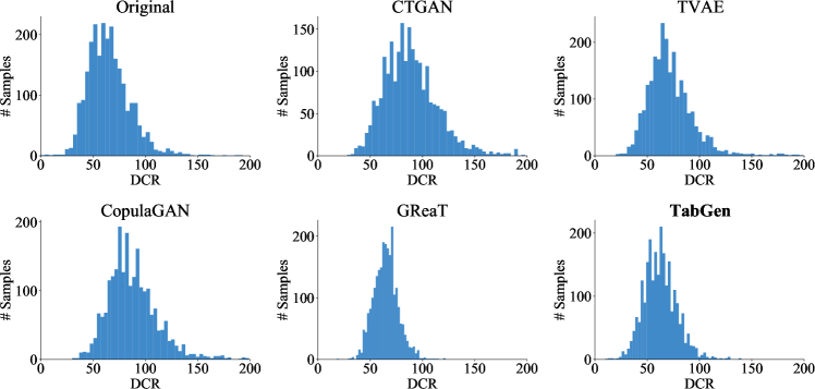
Figure 8: Distance to closest record (DCR) distribution of the HELOC dataset.

References

- Akiba et al. (2019) Takuya Akiba, Shotaro Sano, Toshihiko Yanase, Takeru Ohta, and Masanori Koyama. 2019. Optuna: A next-generation hyperparameter optimization framework. In Proceedings of the 25th ACM SIGKDD International Conference on Knowledge Discovery & Data Mining, KDD 2019, Anchorage, AK, USA, August 4-8, 2019, pages 2623–2631. ACM.
- Alejo et al. (2010) Roberto Alejo, José Martínez Sotoca, Rosa Maria Valdovinos, and P. Toribio. 2010. Edited nearest neighbor rule for improving neural networks classifications. In Advances in Neural Networks - ISNN 2010, 7th International Symposium on Neural Networks, ISNN 2010, Shanghai, China, June 6-9, 2010, Proceedings, Part I, volume 6063 of Lecture Notes in Computer Science, pages 303–310. Springer.
- Andrejczuk et al. (2022) Ewa Andrejczuk, Julian Martin Eisenschlos, Francesco Piccinno, Syrine Krichene, and Yasemin Altun. 2022. Table-to-text generation and pre-training with tabt5. CoRR, abs/2210.09162.
- Arik and Pfister (2021) Sercan Ö. Arik and Tomas Pfister. 2021. Tabnet: Attentive interpretable tabular learning. In Thirty-Fifth AAAI Conference on Artificial Intelligence, AAAI 2021, Thirty-Third Conference on Innovative Applications of Artificial Intelligence, IAAI 2021, The Eleventh Symposium on Educational Advances in Artificial Intelligence, EAAI 2021, Virtual Event, February 2-9, 2021, pages 6679–6687. AAAI Press.
- Asuncion and Newman (2007) Arthur Asuncion and David Newman. 2007. Uci machine learning repository.
- Benjelloun et al. (2020) Omar Benjelloun, Shiyu Chen, and Natasha F. Noy. 2020. Google dataset search by the numbers. In The Semantic Web - ISWC 2020 - 19th International Semantic Web Conference, Athens, Greece, November 2-6, 2020, Proceedings, Part II, volume 12507 of Lecture Notes in Computer Science, pages 667–682. Springer.
- Bhagavatula et al. (2015) Chandra Sekhar Bhagavatula, Thanapon Noraset, and Doug Downey. 2015. Tabel: Entity linking in web tables. In The Semantic Web - ISWC 2015 - 14th International Semantic Web Conference, Bethlehem, PA, USA, October 11-15, 2015, Proceedings, Part I, volume 9366 of Lecture Notes in Computer Science, pages 425–441. Springer.
- Borisov et al. (2022) Vadim Borisov, Kathrin Seßler, Tobias Leemann, Martin Pawelczyk, and Gjergji Kasneci. 2022. Language models are realistic tabular data generators. CoRR, abs/2210.06280.
- Buda et al. (2018) Mateusz Buda, Atsuto Maki, and Maciej A. Mazurowski. 2018. A systematic study of the class imbalance problem in convolutional neural networks. Neural Networks, 106:249–259.
- Camino et al. (2020) Ramiro Daniel Camino, Radu State, and Christian A. Hammerschmidt. 2020. Oversampling tabular data with deep generative models: Is it worth the effort? In "I Can’t Believe It’s Not Better!" at NeurIPS Workshops, Virtual, December 12, 2020, volume 137 of Proceedings of Machine Learning Research, pages 148–157. PMLR.
- Cao et al. (2019) Kaidi Cao, Colin Wei, Adrien Gaidon, Nikos Aréchiga, and Tengyu Ma. 2019. Learning imbalanced datasets with label-distribution-aware margin loss. In Advances in Neural Information Processing Systems 32: Annual Conference on Neural Information Processing Systems 2019, NeurIPS 2019, December 8-14, 2019, Vancouver, BC, Canada, pages 1565–1576.
- Chawla et al. (2002) Nitesh V. Chawla, Kevin W. Bowyer, Lawrence O. Hall, and W. Philip Kegelmeyer. 2002. SMOTE: synthetic minority over-sampling technique. J. Artif. Intell. Res., 16:321–357.
- Chen and Guestrin (2016) Tianqi Chen and Carlos Guestrin. 2016. Xgboost: A scalable tree boosting system. In Proceedings of the 22nd ACM SIGKDD International Conference on Knowledge Discovery and Data Mining, San Francisco, CA, USA, August 13-17, 2016, pages 785–794. ACM.
- Choi et al. (2017) Edward Choi, Siddharth Biswal, Bradley A. Malin, Jon Duke, Walter F. Stewart, and Jimeng Sun. 2017. Generating multi-label discrete patient records using generative adversarial networks. In Proceedings of the Machine Learning for Health Care Conference, MLHC 2017, Boston, Massachusetts, USA, 18-19 August 2017, volume 68 of Proceedings of Machine Learning Research, pages 286–305. PMLR.
- Credit Fusion (2011) Will Cukierski Credit Fusion. 2011. Give me some credit.
- Darabi and Elor (2021) Sajad Darabi and Yotam Elor. 2021. Synthesising multi-modal minority samples for tabular data. CoRR, abs/2105.08204.
- Deng et al. (2021) Xiang Deng, Ahmed Hassan Awadallah, Christopher Meek, Oleksandr Polozov, Huan Sun, and Matthew Richardson. 2021. Structure-grounded pretraining for text-to-SQL. In Proceedings of the 2021 Conference of the North American Chapter of the Association for Computational Linguistics: Human Language Technologies, pages 1337–1350, Online. Association for Computational Linguistics.
- Devlin et al. (2019) Jacob Devlin, Ming-Wei Chang, Kenton Lee, and Kristina Toutanova. 2019. BERT: Pre-training of deep bidirectional transformers for language understanding. In Proceedings of the 2019 Conference of the North American Chapter of the Association for Computational Linguistics: Human Language Technologies, Volume 1 (Long and Short Papers), pages 4171–4186, Minneapolis, Minnesota. Association for Computational Linguistics.
- Dong et al. (2022) Haoyu Dong, Zhoujun Cheng, Xinyi He, Mengyu Zhou, Anda Zhou, Fan Zhou, Ao Liu, Shi Han, and Dongmei Zhang. 2022. Table pre-training: A survey on model architectures, pre-training objectives, and downstream tasks. In Proceedings of the Thirty-First International Joint Conference on Artificial Intelligence, IJCAI 2022, Vienna, Austria, 23-29 July 2022, pages 5426–5435. ijcai.org.
- Eisenschlos et al. (2020) Julian Eisenschlos, Syrine Krichene, and Thomas Müller. 2020. Understanding tables with intermediate pre-training. In Findings of the Association for Computational Linguistics: EMNLP 2020, pages 281–296, Online. Association for Computational Linguistics.
- Gascón et al. (2017) Adrià Gascón, Phillipp Schoppmann, Borja Balle, Mariana Raykova, Jack Doerner, Samee Zahur, and David Evans. 2017. Privacy-preserving distributed linear regression on high-dimensional data. Proc. Priv. Enhancing Technol., 2017(4):345–364.
- Gong et al. (2020) Heng Gong, Yawei Sun, Xiaocheng Feng, Bing Qin, Wei Bi, Xiaojiang Liu, and Ting Liu. 2020. TableGPT: Few-shot table-to-text generation with table structure reconstruction and content matching. In Proceedings of the 28th International Conference on Computational Linguistics, pages 1978–1988, Barcelona, Spain (Online). International Committee on Computational Linguistics.
- Gorishniy et al. (2022) Yury Gorishniy, Ivan Rubachev, and Artem Babenko. 2022. On embeddings for numerical features in tabular deep learning. CoRR, abs/2203.05556.
- Gorishniy et al. (2021) Yury Gorishniy, Ivan Rubachev, Valentin Khrulkov, and Artem Babenko. 2021. Revisiting deep learning models for tabular data. In Advances in Neural Information Processing Systems 34: Annual Conference on Neural Information Processing Systems 2021, NeurIPS 2021, December 6-14, 2021, virtual, pages 18932–18943.
- Grinsztajn et al. (2022) Léo Grinsztajn, Edouard Oyallon, and Gaël Varoquaux. 2022. Why do tree-based models still outperform deep learning on tabular data? CoRR, abs/2207.08815.
- Han et al. (2005) Hui Han, Wenyuan Wang, and Binghuan Mao. 2005. Borderline-smote: A new over-sampling method in imbalanced data sets learning. In Advances in Intelligent Computing, International Conference on Intelligent Computing, ICIC 2005, Hefei, China, August 23-26, 2005, Proceedings, Part I, volume 3644 of Lecture Notes in Computer Science, pages 878–887. Springer.
- He et al. (2008) Haibo He, Yang Bai, Edwardo A. Garcia, and Shutao Li. 2008. ADASYN: adaptive synthetic sampling approach for imbalanced learning. In Proceedings of the International Joint Conference on Neural Networks, IJCNN 2008, part of the IEEE World Congress on Computational Intelligence, WCCI 2008, Hong Kong, China, June 1-6, 2008, pages 1322–1328. IEEE.
- Hegselmann et al. (2022) Stefan Hegselmann, Alejandro Buendia, Hunter Lang, Monica Agrawal, Xiaoyi Jiang, and David A. Sontag. 2022. Tabllm: Few-shot classification of tabular data with large language models. CoRR, abs/2210.10723.
- Herzig et al. (2020) Jonathan Herzig, Pawel Krzysztof Nowak, Thomas Müller, Francesco Piccinno, and Julian Eisenschlos. 2020. TaPas: Weakly supervised table parsing via pre-training. In Proceedings of the 58th Annual Meeting of the Association for Computational Linguistics, pages 4320–4333, Online. Association for Computational Linguistics.
- Jarrett et al. (2022) Daniel Jarrett, Bogdan Cebere, Tennison Liu, Alicia Curth, and Mihaela van der Schaar. 2022. Hyperimpute: Generalized iterative imputation with automatic model selection. In International Conference on Machine Learning, ICML 2022, 17-23 July 2022, Baltimore, Maryland, USA, volume 162 of Proceedings of Machine Learning Research, pages 9916–9937. PMLR.
- Ke et al. (2017) Guolin Ke, Qi Meng, Thomas Finley, Taifeng Wang, Wei Chen, Weidong Ma, Qiwei Ye, and Tie-Yan Liu. 2017. Lightgbm: A highly efficient gradient boosting decision tree. In Advances in Neural Information Processing Systems 30: Annual Conference on Neural Information Processing Systems 2017, December 4-9, 2017, Long Beach, CA, USA, pages 3146–3154.
- Kohavi (1996) Ron Kohavi. 1996. Scaling up the accuracy of naive-bayes classifiers: A decision-tree hybrid. In Proceedings of the Second International Conference on Knowledge Discovery and Data Mining (KDD-96), Portland, Oregon, USA, pages 202–207. AAAI Press.
- Koivu et al. (2020) Aki Koivu, Mikko Sairanen, Antti Airola, and Tapio Pahikkala. 2020. Synthetic minority oversampling of vital statistics data with generative adversarial networks. J. Am. Medical Informatics Assoc., 27(11):1667–1674.
- Koklu and Özkan (2020) Murat Koklu and Ilker Ali Özkan. 2020. Multiclass classification of dry beans using computer vision and machine learning techniques. Comput. Electron. Agric., 174:105507.
- Levin et al. (2022) Roman Levin, Valeriia Cherepanova, Avi Schwarzschild, Arpit Bansal, C. Bayan Bruss, Tom Goldstein, Andrew Gordon Wilson, and Micah Goldblum. 2022. Transfer learning with deep tabular models. CoRR, abs/2206.15306.
- Lewis et al. (2020) Mike Lewis, Yinhan Liu, Naman Goyal, Marjan Ghazvininejad, Abdelrahman Mohamed, Omer Levy, Veselin Stoyanov, and Luke Zettlemoyer. 2020. BART: Denoising sequence-to-sequence pre-training for natural language generation, translation, and comprehension. In Proceedings of the 58th Annual Meeting of the Association for Computational Linguistics, pages 7871–7880, Online. Association for Computational Linguistics.
- Liu et al. (2022) Qian Liu, Bei Chen, Jiaqi Guo, Morteza Ziyadi, Zeqi Lin, Weizhu Chen, and Jian-Guang Lou. 2022. TAPEX: table pre-training via learning a neural SQL executor. In The Tenth International Conference on Learning Representations, ICLR 2022, Virtual Event, April 25-29, 2022. OpenReview.net.
- Ma et al. (2020) Chao Ma, Sebastian Tschiatschek, Richard E. Turner, José Miguel Hernández-Lobato, and Cheng Zhang. 2020. VAEM: a deep generative model for heterogeneous mixed type data. In Advances in Neural Information Processing Systems 33: Annual Conference on Neural Information Processing Systems 2020, NeurIPS 2020, December 6-12, 2020, virtual.
- Mattei and Frellsen (2019) Pierre-Alexandre Mattei and Jes Frellsen. 2019. MIWAE: deep generative modelling and imputation of incomplete data sets. In Proceedings of the 36th International Conference on Machine Learning, ICML 2019, 9-15 June 2019, Long Beach, California, USA, volume 97 of Proceedings of Machine Learning Research, pages 4413–4423. PMLR.
- Mottini et al. (2018) Alejandro Mottini, Alix Lheritier, and Rodrigo Acuna-Agost. 2018. Airline passenger name record generation using generative adversarial networks. CoRR, abs/1807.06657.
- Muzellec et al. (2020) Boris Muzellec, Julie Josse, Claire Boyer, and Marco Cuturi. 2020. Missing data imputation using optimal transport. In Proceedings of the 37th International Conference on Machine Learning, ICML 2020, 13-18 July 2020, Virtual Event, volume 119 of Proceedings of Machine Learning Research, pages 7130–7140. PMLR.
- Naeem et al. (2020) Muhammad Ferjad Naeem, Seong Joon Oh, Youngjung Uh, Yunjey Choi, and Jaejun Yoo. 2020. Reliable fidelity and diversity metrics for generative models. In Proceedings of the 37th International Conference on Machine Learning, ICML 2020, 13-18 July 2020, Virtual Event, volume 119 of Proceedings of Machine Learning Research, pages 7176–7185. PMLR.
- Pace and Barry (1997) R Kelley Pace and Ronald Barry. 1997. Sparse spatial autoregressions. Statistics & Probability Letters, 33(3):291–297.
- Park et al. (2018) Noseong Park, Mahmoud Mohammadi, Kshitij Gorde, Sushil Jajodia, Hongkyu Park, and Youngmin Kim. 2018. Data synthesis based on generative adversarial networks. Proc. VLDB Endow., 11(10):1071–1083.
- Patki et al. (2016) Neha Patki, Roy Wedge, and Kalyan Veeramachaneni. 2016. The synthetic data vault. In 2016 IEEE International Conference on Data Science and Advanced Analytics, DSAA 2016, Montreal, QC, Canada, October 17-19, 2016, pages 399–410. IEEE.
- Pi et al. (2022) Xinyu Pi, Qian Liu, Bei Chen, Morteza Ziyadi, Zeqi Lin, Yan Gao, Qiang Fu, Jian-Guang Lou, and Weizhu Chen. 2022. Reasoning like program executors. CoRR, abs/2201.11473.
- Prokhorenkova et al. (2018) Liudmila Ostroumova Prokhorenkova, Gleb Gusev, Aleksandr Vorobev, Anna Veronika Dorogush, and Andrey Gulin. 2018. Catboost: unbiased boosting with categorical features. In Advances in Neural Information Processing Systems 31: Annual Conference on Neural Information Processing Systems 2018, NeurIPS 2018, December 3-8, 2018, Montréal, Canada, pages 6639–6649.
- Quinlan (1987) J. Ross Quinlan. 1987. Simplifying decision trees. Int. J. Man Mach. Stud., 27(3):221–234.
- Radford et al. (2019) Alec Radford, Jeffrey Wu, Rewon Child, David Luan, Dario Amodei, Ilya Sutskever, et al. 2019. Language models are unsupervised multitask learners. OpenAI blog, 1(8):9.
- Raffel et al. (2020) Colin Raffel, Noam Shazeer, Adam Roberts, Katherine Lee, Sharan Narang, Michael Matena, Yanqi Zhou, Wei Li, and Peter J. Liu. 2020. Exploring the limits of transfer learning with a unified text-to-text transformer. J. Mach. Learn. Res., 21:140:1–140:67.
- Sanh et al. (2019) Victor Sanh, Lysandre Debut, Julien Chaumond, and Thomas Wolf. 2019. Distilbert, a distilled version of BERT: smaller, faster, cheaper and lighter. CoRR, abs/1910.01108.
- Shwartz-Ziv and Armon (2022) Ravid Shwartz-Ziv and Amitai Armon. 2022. Tabular data: Deep learning is not all you need. Inf. Fusion, 81:84–90.
- Sidhu (2021) Gursewak Singh Sidhu. 2021. Crab age prediction.
- Song et al. (2019) Weiping Song, Chence Shi, Zhiping Xiao, Zhijian Duan, Yewen Xu, Ming Zhang, and Jian Tang. 2019. Autoint: Automatic feature interaction learning via self-attentive neural networks. In Proceedings of the 28th ACM International Conference on Information and Knowledge Management, CIKM 2019, Beijing, China, November 3-7, 2019, pages 1161–1170. ACM.
- Stekhoven and Bühlmann (2012) Daniel J. Stekhoven and Peter Bühlmann. 2012. Missforest - non-parametric missing value imputation for mixed-type data. Bioinform., 28(1):112–118.
- Strack et al. (2014) Beata Strack, Jonathan P DeShazo, Chris Gennings, Juan L Olmo, Sebastian Ventura, Krzysztof J Cios, and John N Clore. 2014. Impact of hba1c measurement on hospital readmission rates: analysis of 70,000 clinical database patient records. BioMed research international, 2014.
- Tang et al. (2021) Nan Tang, Ju Fan, Fangyi Li, Jianhong Tu, Xiaoyong Du, Guoliang Li, Samuel Madden, and Mourad Ouzzani. 2021. RPT: relational pre-trained transformer is almost all you need towards democratizing data preparation. Proc. VLDB Endow., 14(8):1254–1261.
- Van Buuren and Groothuis-Oudshoorn (2011) Stef Van Buuren and Karin Groothuis-Oudshoorn. 2011. mice: Multivariate imputation by chained equations in r. Journal of statistical software, 45:1–67.
- Vanschoren et al. (2013) Joaquin Vanschoren, Jan N. van Rijn, Bernd Bischl, and Luís Torgo. 2013. Openml: networked science in machine learning. SIGKDD Explor., 15(2):49–60.
- Wallace et al. (2019) Eric Wallace, Yizhong Wang, Sujian Li, Sameer Singh, and Matt Gardner. 2019. Do NLP models know numbers? probing numeracy in embeddings. In Proceedings of the 2019 Conference on Empirical Methods in Natural Language Processing and the 9th International Joint Conference on Natural Language Processing, EMNLP-IJCNLP 2019, Hong Kong, China, November 3-7, 2019, pages 5306–5314. Association for Computational Linguistics.
- Wang et al. (2021a) Ruoxi Wang, Rakesh Shivanna, Derek Zhiyuan Cheng, Sagar Jain, Dong Lin, Lichan Hong, and Ed H. Chi. 2021a. DCN V2: improved deep & cross network and practical lessons for web-scale learning to rank systems. In WWW ’21: The Web Conference 2021, Virtual Event / Ljubljana, Slovenia, April 19-23, 2021, pages 1785–1797. ACM / IW3C2.
- Wang et al. (2021b) Zhiruo Wang, Haoyu Dong, Ran Jia, Jia Li, Zhiyi Fu, Shi Han, and Dongmei Zhang. 2021b. TUTA: tree-based transformers for generally structured table pre-training. In KDD ’21: The 27th ACM SIGKDD Conference on Knowledge Discovery and Data Mining, Virtual Event, Singapore, August 14-18, 2021, pages 1780–1790. ACM.
- Wang and Sun (2022) Zifeng Wang and Jimeng Sun. 2022. Transtab: Learning transferable tabular transformers across tables. CoRR, abs/2205.09328.
- Wolf et al. (2019) Thomas Wolf, Lysandre Debut, Victor Sanh, Julien Chaumond, Clement Delangue, Anthony Moi, Pierric Cistac, Tim Rault, Rémi Louf, Morgan Funtowicz, and Jamie Brew. 2019. Huggingface’s transformers: State-of-the-art natural language processing. CoRR, abs/1910.03771.
- Xing and Wan (2021) Xinyu Xing and Xiaojun Wan. 2021. Structure-aware pre-training for table-to-text generation. In Findings of the Association for Computational Linguistics: ACL-IJCNLP 2021, pages 2273–2278, Online. Association for Computational Linguistics.
- Xu et al. (2019) Lei Xu, Maria Skoularidou, Alfredo Cuesta-Infante, and Kalyan Veeramachaneni. 2019. Modeling tabular data using conditional GAN. In Advances in Neural Information Processing Systems 32: Annual Conference on Neural Information Processing Systems 2019, NeurIPS 2019, December 8-14, 2019, Vancouver, BC, Canada, pages 7333–7343.
- Yin et al. (2020) Pengcheng Yin, Graham Neubig, Wen-tau Yih, and Sebastian Riedel. 2020. TaBERT: Pretraining for joint understanding of textual and tabular data. In Proceedings of the 58th Annual Meeting of the Association for Computational Linguistics, pages 8413–8426, Online. Association for Computational Linguistics.
- Yoon et al. (2018) Jinsung Yoon, James Jordon, and Mihaela van der Schaar. 2018. GAIN: missing data imputation using generative adversarial nets. In Proceedings of the 35th International Conference on Machine Learning, ICML 2018, Stockholmsmässan, Stockholm, Sweden, July 10-15, 2018, volume 80 of Proceedings of Machine Learning Research, pages 5675–5684. PMLR.
- Yu et al. (2021) Tao Yu, Chien-Sheng Wu, Xi Victoria Lin, Bailin Wang, Yi Chern Tan, Xinyi Yang, Dragomir R. Radev, Richard Socher, and Caiming Xiong. 2021. Grappa: Grammar-augmented pre-training for table semantic parsing. In 9th International Conference on Learning Representations, ICLR 2021, Virtual Event, Austria, May 3-7, 2021. OpenReview.net.
- Zeng et al. (2016) Min Zeng, Beiji Zou, Faran Wei, Xiyao Liu, and Lei Wang. 2016. Effective prediction of three common diseases by combining smote with tomek links technique for imbalanced medical data. In 2016 IEEE International Conference of Online Analysis and Computing Science (ICOACS), pages 225–228. IEEE.
- Zhang et al. (2022) Tianping Zhang, Zheyu Zhang, Zhiyuan Fan, Haoyan Luo, Fengyuan Liu, Wei Cao, and Jian Li. 2022. Openfe: Automated feature generation beyond expert-level performance. CoRR, abs/2211.12507.