Isotropic stellar model in mimetic theory

Abstract

We investigate how to derive an isotropic stellar model in the framework of mimetic gravitational theory. Recently, this theory has gained big interest due to its difference from Einstein’s general relativity (GR), especially in the domain non-vacuum solutions. In this regard, we apply the field equation of mimetic gravitational theory to a spherically symmetric ansatz and obtain an over determined system of non-linear differential equations in which differential equations are less than the unknown functions. To overcome the over determined system we suppose a specific form of the temporal component of the metric potential, $g_{tt}$, and assume the vanishing of the anisotropic condition to derive the form of the spatial component of the metric, $g_{rr}$. In this regard, we discuss the possibility to derive a stellar isotropic model that is in agreement with observed pulsars. To examine the stability of the isotropic model we use the Tolman-Oppenheimer-Volkoff equation and the adiabatic index. Furthermore, we assess the model’s validity by evaluating its compatibility with a broad range of observed pulsar masses and radii. We demonstrate that the model provides a good fit to these observations.

I Introduction

The theory of General Relativity (GR) was constructed by Einstein in (1915) and is considered one of the basic theories of modern physics as well as the quantum field theory Carroll et al. (2004). Up to date, GR has approved many successful tests in experimental as well as observational like gravitational time dilation, bending of light, the precession of the Mercury orbit, gravitational lensing, etc Will (2006), and the discovery of the gravitational waves Abbott et al. (2016). In spite the huge progress of GR, it endures investigating the issues of cosmological observations like the flat galaxy’s rotation curves (dark matter), the black holes singularities as well as the accelerated expansion era of the universe (dark energy). Thus, new components of matter-energy or modified theories of gravity should be proposed to investigate the observed events.

Mimetic gravitational theory is a scalar-tensor one where the conformal mode can be isolated through a scalar field Chamseddine and Mukhanov (2013). On the other hand, we can think of the setup of the mimetic as a special class of general conformal or disformal transformation where the transformation between the new and old metrics is degenerate. Using the non-invertible conformal or disformal transformation one can prove that the number of degrees of freedom can be increased so that the longitudinal mode becomes dynamical Deruelle and Rua (2014); Domènech et al. (2015); Firouzjahi et al. (2018); Shen et al. (2019). The conformal transformation which relates the auxiliary metric ${\bar{g}}_{\alpha\beta}$ to the physical metric $g_{\alpha\beta}$ and the scalar field is defined as:

$$g_{\alpha\beta}=\pm\left(\bar{g}^{\mu\nu}\partial_{\mu}\zeta\partial_{\nu}\zeta\right)\bar{g}_{\alpha\beta}\,.$$ (1)

We stress that the physical metric $g_{\alpha\beta}$ is invariant using the conformal transformation of the auxiliary metric $\bar{g}^{\alpha\beta}$. This invariance fixes in a unique way the form of the conformal factor w.r.t. the auxiliary metric $\bar{g}^{\mu\nu}$ and the scalar field $\zeta$ however such transformation cannot fix the sign. Equation (1) yields that the following condition:

$$g^{\alpha\beta}\partial_{\alpha}\zeta\partial_{\beta}\zeta=\pm 1\,.$$ (2)

Equation (2) shows that $\partial_{\beta}\zeta$ is a timelike for the $-$ sign and spacelike for the $+$ sign. The $-$ sign in Eqs. (1) and (2) is the original sign of standard mimetic gravity Chamseddine and Mukhanov (2013) however the $+$ sign is a generalization of the mimetic gravity. An amended type of mimetic gravity can process the cosmological singularities Chamseddine and Mukhanov (2017a) and the singularity in the core of a black hole Chamseddine and Mukhanov (2017b). Furthermore, the initial attempt of the mimetic theory provides a guarantee that gravitational waves (GW) can travel at the speed of light, thereby supporting the consistency observed in recent findings such as the event GW170817 and its corresponding optical counterpart Casalino et al. (2018, 2019); Sherafati et al. (2021). Moreover, mimetic theory can investigate the flat rotation curves of spiral galaxies without the need of dark matter Vagnozzi (2017); Sheykhi and Grunau (2021). From a cosmological point of view, the theory of mimetic has discussed a lot of interesting research papers in the past few years Chamseddine et al. (2014); Baffou et al. (2017); Dutta et al. (2018); Sheykhi (2018); Abbassi et al. (2018); Matsumoto (2016); Sebastiani et al. (2017); Sadeghnezhad and Nozari (2017); Gorji et al. (2019, 2018a); Bouhmadi-López et al. (2017); Gorji et al. (2018b); Chamseddine et al. (2019a); Russ (2021); de Cesare et al. (2020); Farsi and Sheykhi (2022); Cárdenas et al. (2021); Hosseini Mansoori et al. (2021); Arroja et al. (2018) and black holes physics Gorji et al. (2020); Myrzakulov and Sebastiani (2015); Nashed and El Hanafy (2017); Nashed (2011); Myrzakulov et al. (2016); Ganz et al. (2019); Chen et al. (2018); Nashed (2018a); Ben Achour et al. (2018); Brahma et al. (2018); Zheng et al. (2017, 2017); Nashed et al. (2019); Chamseddine et al. (2019b); Gorji et al. (2020); Sheykhi (2020, 2021); Nashed and Nojiri (2021); Chamseddine (2021); Bakhtiarizadeh (2021); Nashed (2021). It has been shown that for a spherically symmetric spacetime the only solution is the Schwarzschild spacetime which means that the Birkhoff’s theorem is hold. Moreover, mimetic theory have been extended to $f(R)$ gravity Nojiri and Odintsov (2014); Odintsov and Oikonomou (2016a); Oikonomou (2016a, b, c); Myrzakulov and Sebastiani (2016); Odintsov and Oikonomou (2015, 2016b, 2016c); Nojiri et al. (2017a); Odintsov and Oikonomou (2018); Bhattacharjee (2021); Kaczmarek and Szczesniak (2021); Chen et al. (2021) and to Gauss-Bonnet gravitational theory Astashenok et al. (2015); Oikonomou (2015); Zhong and Elizalde (2016); Zhong and Sáez-Chillón Gómez (2018); Paul et al. (2020). More specifically, a unified scenario of early inflation and late-time acceleration in the framework of mimetic $f(R)$ gravity was formulated in Nojiri et al. (2016). Moreover, it was assured that in the frame of mimetic $f(R)$ gravity, the inflationary epoch can be discussed Nojiri et al. (2016). In the present study we discuss the interior of spherically symmetric solution within mimetic gravitational theory. Because of the non-trivial contribution of the mimetic field $\zeta$ the Einstein field equation gives:

$${G_{\mu\nu}+\frac{1}{2}g_{\mu\nu}(\partial^{\mu}\zeta\partial^{\nu}\zeta+1)=\kappa T_{\mu\nu}}\,,$$ (3)

where $T_{\mu\nu}$ is the energy-momentum tensor and $\kappa=\frac{8\pi\,G}{c^{4}}$ is the gravitational constant and $G_{\mu\nu}$ is the Einstein tensor defined as:

$${G_{\mu\nu}=R_{\mu\nu}-\frac{1}{2}G_{\mu\nu}R}\,,$$ (4)

where $R_{\mu\nu}$ is the Ricci tensor defined as:

$${R_{\mu\nu}={R^{\alpha}}_{\mu\alpha\nu}={\Gamma^{\alpha}}_{\mu\nu,\alpha}-{\Gamma^{\alpha}}_{\mu\alpha,\nu}+{\Gamma^{\alpha}}_{\nu\mu}{\Gamma^{\beta}}_{\alpha\beta}-{\Gamma^{\alpha}}_{\nu\beta}{\Gamma^{\beta}}_{\alpha\mu}}\,,$$

with ${\Gamma^{\alpha}}_{\nu\mu}$ being the Christoffel symbols second kind and ${R^{\alpha}}_{\mu\alpha\nu}$ is the Riemann tensor fourth order and $R$ is the Ricci scalar defined as $R=g^{\mu\nu}R_{\mu\nu}$. Equations (3) coincides with Einstein GR when the scalar field has a constant value, i.e., $\partial^{\mu}\zeta\partial^{\nu}\zeta+1=0$. There are many applications in the framework of mimetic in cosmology as well as in solar system (see for example Saadi, 2016; Haghani et al., 2015; Addazi and Marciano, 2017; Astashenok and Odintsov, 2016; Babichev and Ramazanov, 2017).

The current study is structured as follows: In Section II, we utilize mimetic field equations, specifically equation (3), to analyze a spherically symmetric object with an anisotropic matter source. This results in a system of three nonlinear differential equations with five unknown functions, including two metric potentials, energy density, radial pressure, and tangential pressure. To close the system, we impose two additional constraints: we assume a specific form for one of the metric potentials, $g_{tt}$, which is commonly done in interior solutions, and we assume the vanishing of anisotropy and derive the form of the spatial component of the metric potential, $g_{rr}$. Collecting this information, we obtain the analytic expressions for the energy density and pressure that satisfy the mimetic equation of motion. In subsection II.1, we delineate the physical requirements that any isotropic stellar model must meet to be in agreement with a genuine compact star. In Section III, we discuss the applicability of the derived solution under the conditions presented in Section II.1. In Section IV, We integrate our model using the Schwarzschild solution, an external vacuum solution, and make adjustments the model parameters based on the properties of the pulsar Cen X-3, which has a mass estimate of $M=1.49\pm 0.49,M_{\odot}$ and a radius of $R=9.178\pm 0.13$ km. In Section V, we investigate the stability of the model using the TOV equation of hydrostatic equilibrium and the adiabatic index. Finally, we summarize our findings in Section VI.

II spherically symmetric interior solution

To be able to derive an interior solution we will use a spherically symmetric spacetime to make the calculations and discussion more easy. For this aim, we assume the spacetime of spherical symmetric to have the form:

$$ds^{2}=E^{2}(r)dt^{2}-\frac{1}{E_{1}(r)}\,dr^{2}-r^{2}(d\theta^{2}-\sin^{2}\theta d\phi^{2})\,,$$ (5)

with $E(r)$ and $E_{1}(r)$ are unknown functions. When $E=E_{1}$ one can recover Schwarzschild solution for exterior Einstein GR. Using Eq. (5), we get the Ricci tensor and Ricci scalar in the form:

$${{\mathcal{R}}_{tt}(r)=\frac{E(2rE_{1}E^{\prime\prime}+E^{\prime}[rE^{\prime}_{1}+4E_{1}])}{2r}}\,,$$

$${{\mathcal{R}}_{rr}(r)=-\frac{2rE_{1}E^{\prime\prime}+E^{\prime}_{1}[rE^{\prime}+2E])}{2EE_{1}r}}\,,$$

$${{\mathcal{R}}_{\theta\theta}(r)=-\frac{2rE_{1}E^{\prime}+rEE^{\prime}_{1}-2E(1-E_{1})}{2E}\,,\qquad{\mathcal{R}}_{\phi\phi}(r)={\mathcal{R}}_{\theta\theta}(r)\sin^{2}\theta}\,,$$

$${{\mathcal{R}}(r)=-\frac{E^{\prime}E^{\prime}_{1}{r}^{2}+2\,E_{1}E^{\prime\prime}{r}^{2}+4\,E_{1}E^{\prime}r+2\,E^{\prime}_{1}Er-2\,E+2\,EE_{1}}{E{r}^{2}}}\,,$$ (6)

where $E\equiv E(r)$, $E_{1}\equiv E_{1}(r)$, $E^{\prime}=\frac{dE}{dr}$, $E^{\prime\prime}=\frac{d^{2}E}{dr^{2}}$ and $E_{1}^{\prime}=\frac{dE_{1}}{dr}$. Plugging Eq. (3) with Eq. (5) and by using Eq. (II) we get:

The t t component of mimetic field equation is:

$$\rho=\frac{1-rE^{\prime}_{1}-E_{1}}{r^{2}}\,,$$

The r r component of mimetic field equation is:

$$p={\frac{2\,\zeta^{\prime 2}E_{1}{}^{2}{r}^{2}E^{\prime\prime}+\left[r\left(4\,E_{1}+E^{\prime}_{1}r\right)E^{\prime}+E\left(2E_{1}-2+{r}^{2}\rho-3{r}^{2}p+2E^{\prime}_{1}r\right)\right]E_{1}\zeta^{\prime 2}+2E^{\prime}rE_{1}+E\left(E_{1}-1\right)}{E{r}^{2}}}\,,$$

$$\textrm{ The}\,\mathrm{\theta\,\theta=\phi\,\phi}\textrm{ component of Mimetic field equation is:}$$

$$p_{1}=\frac{2rE_{1}E^{\prime\prime}+2E_{1}E^{\prime}+E^{\prime}_{1}(E+rE^{\prime})}{2E{r}}\,,$$

(7)

where we have set the Einstein gravitational constant, i.e., $\kappa$, to unity. For an anisotropic fluid with spherical symmetry, we assume the energy-momentum tensor., i.e.

$${{T}{{}^{\alpha}}{{}_{\beta}}=(p_{1}+\rho)u{{}^{\alpha}}u{{}_{\beta}}+p_{1}\delta^{\alpha}_{\beta}+(p-p_{1})\chi{{}^{\alpha}}\chi{{}_{\beta}}\,.}$$ (8)

Here, $\rho=\rho(r)$ represents the energy density of the fluid, $p=p(r)$ denotes its radial pressure and $p_{1}=p_{1}(r)$ represents the tangential pressure. As a result, the energy-momentum tensor takes the form ${T}{{}^{\alpha}}{\beta}=diag(-\rho,\,p,\,p{1},\,p_{1})$. If the mimetic scalar field has a constant value, or $\zeta=C$, then equations (7) will be equivalent to the interior differential equations of Einstein’s general relativity Nashed et al. (2020); Nashed and Capozziello (2020).. The differential equations (7) are three non-linear in six unknowns $E$, $E_{1}$, $\rho$, $p$, $p_{1}$ and the mimetic field $\zeta$ which we can fix it form the use of Eq. (2), i.e.,

$$\zeta=\frac{1}{\sqrt{-E_{1}}}.$$

Therefore, to put the above system in a solvable form we need two extra conditions. The first one is to suppose the temporal component of the metric potential $E$ in the form Torres-Sánchez and Contreras (2019); Estevez-Delgado et al. (2019):

$$E(r)={\frac{a_{0}\left(5+4\,a_{1}{r}^{2}\right)}{\sqrt{1+a_{1}{r}^{2}}}}\,,$$ (9)

where $a_{0}$ is a constant that has no dimension and $a_{1}$ is another constant that has dimension of inverse length square, i.e., $L^{-2}$. The second condition is the use of r r and $\mathrm{\theta\,\theta}$ components of Eq. (7), i.e., the anisotropy equation, and imposing of Eq. (9) yields:

$$E_{1}(r)=\frac{\left(1+2\,a_{1}{r}^{2}+{a_{1}}^{2}{r}^{4}\right)}{\varepsilon^{3}}\biggl{\{}[5+6\,a_{1}r^{2}]\varepsilon-4\,a_{1}[1+a_{1}{r}^{2}]{r}^{2}\varepsilon_{1}+a_{2}{r}^{2}+a_{2}\,a_{1}{r}^{4}\biggr{\}}\,.$$ (10)

Here $a_{2}$ is a constant of integration with inverse length square dimension, i.e., $L^{-2}$, $\varepsilon=\sqrt{5+12\,a_{1}{r}^{2}+8\,{a_{1}}^{2}{r}^{4}}$ and $\varepsilon_{1}={\mathrm{arctanh}}\left({\frac{1+2\,a_{1}{r}^{2}}{\varepsilon}}\right)$.

Using Eqs. (9) and (10) in the system of differential Eqs. (7), we obtain the components of the energy-momentum in the form:

$$\rho={\frac{1}{\varepsilon^{6}}}\,\biggl{\{}12\,\left(1+a{r}^{2}\right)^{2}\left(\left(3a_{1}{r}^{2}+1\right)\varepsilon^{3}-4\left(3+4a_{1}{r}^{2}\right)\left(1+a_{1}{r}^{2}\right)\varepsilon a_{1}{r}^{2}\right)a_{1}\varepsilon_{1}-3\,\left(1+3a_{1}{r}^{2}\right)\left(1+a_{1}{r}^{2}\right)^{2}a_{2}\,\varepsilon^{3}$$

$$+\biggl{(}12\left(3+4a_{1}{r}^{2}\right)\left(1+a_{1}{r}^{2}\right)^{3}{r}^{2}a_{2}\,\varepsilon+\varepsilon\left(144{a_{1}}^{4}{r}^{8}+424\,{a_{1}}^{3}{r}^{6}+486\,{a_{1}}^{2}{r}^{4}+265\,a_{1}{r}^{2}+60\right)\biggr{)}a_{1}\biggr{\}}\,,$$

$$p={\frac{1}{\varepsilon^{6}\left(5+4a_{1}{r}^{2}\right)}}\,\biggl{\{}\left(36{a_{1}}^{2}{r}^{4}+33\,a_{1}{r}^{2}+5\right)\left(1+a_{1}{r}^{2}\right)^{2}a_{2}\,\varepsilon^{3}-4\left(1+a{r}^{2}\right)^{2}a_{1}\left(12{a_{1}}^{2}{r}^{4}+15\,a_{1}{r}^{2}+5\right)\varepsilon^{3}\varepsilon_{1}$$

$$+\varepsilon^{3}\biggl{(}\varepsilon^{1/2}\left(72{a_{1}}^{3}{r}^{6}+190\,{a_{1}}^{2}{r}^{4}+167\,a_{1}{r}^{2}+50\right)-6\left(3+4a_{1}{r}^{2}\right)\left(1+a_{1}{r}^{2}\right)^{2}{r}^{2}a_{2}\,\biggr{)}a_{1}\biggr{\}}\,.$$

The energy density of Eq. (II) is the same as of GR for isotropic solution Torres-Sánchez and Contreras (2019) however, the pressure is different. This difference is due to the contribution of the mimetic scalar field. It should be noted that if the mimetic scalar field is set equal zero in Eq. (7) and solving the system using ansatz (9) we get the form of density and pressure presented in Torres-Sánchez and Contreras (2019). Moreover, it is important to stress that the use of metric potentials (9) and (10) in the system (7) gives $p=p_{1}$ which insure the isotropy of our model.

The mass contained in a sphere that has radius $r$ is given by:

$$M(r)=4\pi{\int_{0}}^{r}\rho(\eta)\eta^{2}d\eta\,.$$ (12)

By employing the expression for energy density provided in Equation (II) and substituting it into Equation (12), we obtain the asymptotic representation of the mass as:

$$M(r)\approx(-0.3139182118a_{1}-0.04472135955a_{2})r^{3}+a_{1}(0.08835092710a_{1}{}^{2}+0.02683281574a_{1}a_{2})r^{5}$$

$$-a_{1}{}^{2}(0.0883509271a_{1}+0.02683281574a_{2})r^{7}+a_{1}{}^{3}(0.03114573467a_{1}+0.0196773982a_{2})r^{9}\,.$$ (13)

The compactness parameter with radius $r$ of a spherically symmetric source is defined as Newton Singh et al. (2019); Roupas and Nashed (2020):

$$C(r)=\frac{2M(r)}{r}.$$ (14)

In the next subsection, we present the physical conditions that are viable for an isotropic stellar structure and examine if model (II) satisfy them or not.

II.1 Necessary criteria for a physically viable stellar isotropic model

Before we proceed we are going to use the following dimensionless substitution:

$$r=xR\,,$$

where $R$ is the radius of the star and $x$ is a dimensionless constant that equal to one when $r=R$ and equal zero at the center of the star. Also we assume the dimensional constants $a_{1}$ and $a_{2}$ to take the form:

$$a_{1}=\frac{u}{R^{2}}\,,\qquad a_{2}=\frac{w}{R^{2}}.$$ (15)

where $u$ and $w$ are dimensional quantities. By using the substitution of $a_{1}$, $a_{2}$ and $r$ into the physical components of model, Eqs. (9), (10) and (II) we will get a dimensionless physical quantities. Now we are ready to discuss the necessary criteria that we apply in the isotropic model:

A physical isotropic model must verify:
$\bullet$ The metric potentials $E(x)$ and $E_{1}(x)$, and $\rho$ and $p$ must have good behavior at the core of the stellar object and have regular behavior through the structure of the star without singularity.
$\bullet$ The energy density component, denoted as $\rho$, is required to be positive within the internal structure of the star. Additionally, it should possess a finite positive value and exhibit a monotonically decreasing trend towards the surface of the stellar interior, i.e., $\frac{d\rho}{dx}\leq 0$.
$\bullet$ The pressure, denoted as $p$, must maintain a positive value throughout the fluid structure, meaning $p\geq 0$. Furthermore, the derivative of pressure with respect to the spatial variable, i.e., $\frac{dp}{dx}<0$, must be, indicating a decreasing pressure gradient. Additionally, at the surface, $x=1$, (corresponding to $r=R$), the pressure $p$ should be zero.
$\bullet$ The energy conditions of isotropic star requires the following inequalities:
(i)The condition of weak energy (WEC): $p+\rho>0$, $\rho>0$.   (ii) The conditions of dominant energy (DEC): $\rho\geq\lvert p\lvert$.  
(iii) The condition of strong energy (SEC): $p+\rho>0$, $\rho+3p>0$.
$\bullet$ The causality condition must be verified, to have a viable true model, i.e., $v<1$ where $v$ is the speed of sound.
$\bullet$ The interior metric potentials, $E$ and $E_{1}$, must be joined smoothly to the exterior metric potentials (Schwarzschild metric) at the surface of the stellar, i.e., $x=1$.
$\bullet$ For a true star the adiabatic index is greater than $\frac{4}{3}$.

Now, we are ready to examine the above-listed physical criteria on our model to see if it satisfies all of them or not.

III The Physical behaviors of model (II)

III.1 The free singularity of the model

a- The metric potentials given by Eqs (II) and (10) fulfill:

$$E_{x\rightarrow 0}=25a_{0}{}^{2}\,\qquad\qquad\textrm{and}\qquad\qquad{E_{1}}_{x\rightarrow 0}=1\,.$$ (16)

Equation (16) guarantees that the lapse functions possess finite values at the core of the stellar configuration. Additionally, the derivatives of the metric potentials with respect to x must also have finite values at the core, i.e., $f^{\prime}(x=0)=f^{\prime}_{1}(x=0)=0$. Equations (16) ensures that the laps functions are regular at the core and have good behavior throughout the center of the star.
ii-The density and pressure of Eq. (II) take the following form at core:

$${\rho_{{}_{{}_{x\rightarrow 0}}}=\frac{12\,u\sqrt{5}{\mathrm{arctanh}}\left(1/\sqrt{5}\right)-3\,w\sqrt{5}-60\,u}{}{25R}^{2}}\,,$$

$${{p}_{{}_{{}_{x\rightarrow 0}}}=\frac{50\,u-4\,u\sqrt{5}{\mathrm{arctanh}}\left(1/\sqrt{5}\right)+w\sqrt{5}}{{25R}^{2}}}\,.$$ (17)

Equation (III.1) ensures the positivity of density and pressure assuming

$${12\,u\sqrt{5}{\mathrm{arctanh}}\left(1/\sqrt{5}\right)-3\,w\sqrt{5}-60\,u>0\,,\qquad{\textrm{a}nd}\qquad 50\,u-4\,u\sqrt{5}{\mathrm{arctanh}}\left(1/\sqrt{5}\right)+w\sqrt{5}>0}\,.$$

Moreover, the Zeldovich condition Zeldovich and Novikov (1971) that connects the density and pressure at the center of the star through the inequality, i.e., $\frac{p(0)}{\rho(0)}\leq 1$. Applying Zeldovich condition in Eq. (III.1), we get:

$${\frac{50\,u-4\,u\sqrt{5}{\mathrm{arctanh}}\left(1/\sqrt{5}\right)+w\sqrt{5}}{12\,u\sqrt{5}{\mathrm{arctanh}}\left(1/\sqrt{5}\right)-3\,w\sqrt{5}-60\,u}\leq 1}\,,$$ (18)

which yields:

$$\Rightarrow w\leq\frac{\left[8\sqrt{5}{\mathrm{arctanh}}\left(1/\sqrt{5}\right)-55\right]u}{2\sqrt{5}}\,.$$

iii-The derivatives of density, $\rho$, and pressure, $p$, of Eq. (II) are respectively:

$$\rho^{\prime}=-\frac{2\,x{u}^{2}}{{R}^{2}\varepsilon^{7/2}}\biggl{\{}192\,w\,{u}^{5}{x}^{10}+192\,\varepsilon_{1}{u}^{5}{x}^{10}+1248\,\varepsilon_{1}{u}^{4}{x}^{8}-32\,\varepsilon{x}^{4}{u}^{4}{x}^{8}+1248\,w\,{u}^{4}{x}^{8}-96\,\varepsilon{u}^{3}{x}^{6}+3048\,{w}\,{u}^{3}{x}^{6}$$

$$+3048\,\varepsilon_{1}{u}^{3}{x}^{6}-372\,\varepsilon{u}^{2}{x}^{4}+3372\,\varepsilon_{1}{u}^{2}{x}^{4}+3372\,w\,{u}^{2}{x}^{4}-480\,\varepsilon\,u{x}^{2}+1680\,\varepsilon_{1}u{x}^{2}+1680\,w\,u{x}^{2}+300\,w+300\,\varepsilon_{1}-175\,\varepsilon\biggr{\}}\,,$$

$$p^{\prime}=\frac{2\,xw}{\left(5+4\,u{x}^{2}\right)^{2}{R}^{2}\varepsilon^{5/2}}\biggl{\{}96\,w\,{u}^{5}{x}^{10}-384\,{w}^{6}\varepsilon_{1}{x}^{10}+64\,{u}^{5}\zeta{x}^{8}-1792\,{u}^{5}\varepsilon_{1}{x}^{8}+448\,w\,{u}^{4}{x}^{8}+160\,{u}^{4}\varepsilon{x}^{6}-3448\,{u}^{4}\varepsilon_{1}{x}^{6}$$

$$+862\,w\,{u}^{3}{x}^{6}-3340\,{u}^{3}\varepsilon_{1}{x}^{4}+244\,{u}^{3}\varepsilon{x}^{4}+835\,w\,{u}^{2}{x}^{4}-1600\,{u}^{2}\varepsilon_{1}{x}^{2}+220\,{u}^{2}\varepsilon{x}^{2}+400\,w\,u{x}^{2}-300\,u\varepsilon_{1}+75\,u\varepsilon+75\,w\biggr{\}}\,,$$

where $\rho^{\prime}=\frac{d\rho}{dx}$ and $p^{\prime}=\frac{dp_{r}}{dx}$. Fig. 2 1(a) shows that the gradients of the components of energy-momentum tensor behave in negative way.
iv-The speed of sound (when c = 1) yields:

$$v{}^{2}=\frac{dp}{d\rho}=\frac{\varepsilon^{2}}{\left(5+4\,u{x}^{2}\right)^{2}}\bigg{\{}96\,w\,{u}^{5}{x}^{10}-384\,{u}^{6}\varepsilon_{1}{x}^{10}+64\,{u}^{5}\varepsilon{x}^{8}-1792\,{u}^{5}\varepsilon_{1}{x}^{8}+448\,w\,{u}^{4}{x}^{8}+160\,{u}^{4}\varepsilon{x}^{6}-3448\,{u}^{4}\varepsilon_{1}{x}^{6}$$

$$+862\,w\,{u}^{3}{x}^{6}-3340\,{u}^{3}\varepsilon_{1}{x}^{4}+244\,{u}^{3}\varepsilon{x}^{4}+835\,w\,{u}^{2}{x}^{4}-1600\,{u}^{2}\varepsilon_{1}{x}^{2}+220\,{u}^{2}\varepsilon{x}^{2}+400\,w\,u{x}^{2}-300\,u\varepsilon_{1}+75\,u\varepsilon+75\,w\bigg{\}}$$

$$\bigg{\{}48\,w\,{u}^{5}{x}^{10}-192\,{u}^{6}\varepsilon_{1}{x}^{10}+32\,{u}^{5}\varepsilon{x}^{8}-1248\,{u}^{5}\varepsilon_{1}{x}^{8}+312\,w\,{u}^{4}{x}^{8}+96\,{u}^{4}\varepsilon{x}^{6}-3048\,{u}^{4}\varepsilon_{1}{x}^{6}+75\,w$$

$$+762\,w\,{u}^{3}{x}^{6}-3372\,{u}^{3}\varepsilon_{1}{x}^{4}+372\,{u}^{3}\varepsilon{x}^{4}+843\,w\,{u}^{2}{x}^{4}+480\,{u}^{2}\varepsilon{x}^{2}-1680\,{u}^{2}\varepsilon_{1}{x}^{2}+420\,w\,u{x}^{2}+175\,u\varepsilon-300\,u\varepsilon_{1}\biggr{\}}^{-1}\,.$$

which is less than unity as Fig. 2 1(b) shows.

III.2 Junction conditions

We make the assumption that the exterior solution of the star is a vacuum, described by the Schwarzschild solution. This is because, in the mimetic theory, the Schwarzschild solution is the only exterior spherically symmetric solution Nashed et al. (2020); Nashed and Capozziello (2020). The form of the Schwarzschild solution is given by:

$$ds^{2}=-\Big{(}1-\frac{2M}{xR}\Big{)}dt^{2}+\Big{(}1-\frac{2M}{xR}\Big{)}^{-1}dr^{2}+x^{2}R^{2}d\Omega^{2},$$ (23)

where $M$ is the mass of the star. The junction of the laps functions at $x=1$ gives:

$$E(x\rightarrow 1)=\left(1-\frac{2M}{R}\right),\qquad\qquad E_{1}(x\rightarrow 1)=\left(1-\frac{2M}{R}\right)^{-1}\,,$$ (24)

in addition to the constrain of the vanishing of pressure at the surface we fix the dimensionless constants of solution (9) and (10) as:

$$a_{0}=\pm{\frac{\sqrt{R\left(R+R{u}^{2}-2\,M-2\,M{u}^{2}\right)}}{R\left(5+4\,{u}^{2}\right)}}\,,$$

$$u=-\frac{48\,\sqrt{2}M+R\left[19\sqrt{2}-9\,R\,\varrho\right]-\sqrt{M\left[4608\,{M}-864\,\sqrt{2}R+3648R\right]+[351\,\varrho^{2}-1482\,\varrho\sqrt{2}+2702]\,{R}^{2}}}{24R\left(3\,\sqrt{2}-\varrho\right)}\,,$$

$$w={\frac{u\left[4\left(u+1\right)^{2}\left(12{u}^{2}+15u+5\right)\varepsilon_{1}-\left(72{u}^{3}+190\,{u}^{2}+167\,u+50\right)\varepsilon\right]}{\left(47\,{u}^{2}+39\,{u}^{3}+12\,{u}^{4}+25\,u+5\right)}}\,,$$

where $\varrho=\mathrm{arctanh}\left(\frac{1}{\sqrt{2}}\right)$.

IV Examination of the model (II) with true compact stars

Now, we are ready to use the previously listed conditions in Eq. (II) to examine the physical masses and radii of the stars. To extract more information of the model (II), we use the pulsar Cen X-3 which has mass $M=1.49\pm 0.49M_{\circledcirc}$ and radius $R=9.178\pm 0.13$ km, respectively Gangopadhyay et al. (2013). In this study the value of mass is $M=1.98M_{\circledcirc}$ and the radius is $R=9.308km$. These conditions fix the dimensionless constants $a_{0}$, $u$ and $w$ as:

$$a_{0}=-0.1509026812\,,\qquad\qquad u=0.1241376545\,,\qquad w=-2.382227207\,.$$ (26)

Using the above values of constants we plot the physical quantities of the model (II).

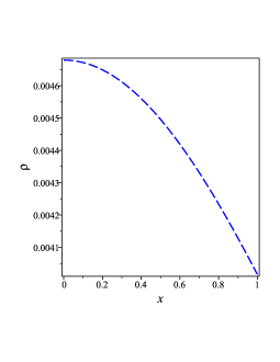
(a)  Energy-density given by Eq. (II)

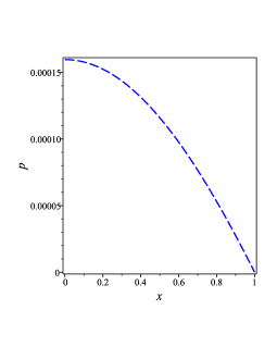
(b)   Pressure given by Eq. (II)

Figure 1: Plots of Fig. 0(a) the density and Fig. 0(b) pressure of (II) versus the dimensionless $x$ using the constants fixed from Cen X-3 Naik et al. (2011).

In Figs. 1 0(a), and 0(b) we depict energy-density and pressure of the star Cen X-3 which shows that density and pressure possess positive values as necessary for true stellar configuration moreover, the density is high at the center and decreases toward the surface of the star. additionally, Fig. 1 0(b) shows that the value of the pressure is zero at the surface of the stellar. The behaviors of density and pressure presented in Figs. 1 0(a), and 0(b) are appropriate to a true model.

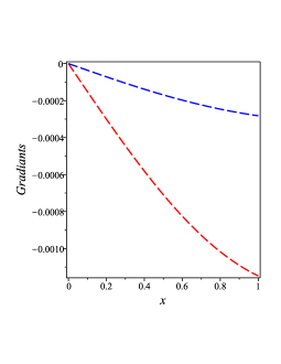
(a)  Speed of sound

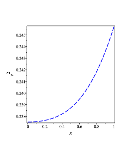
(b)  Weak energy conditions

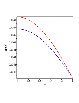
(c)  Weak energy conditions

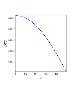
(d)  Strong energy condition

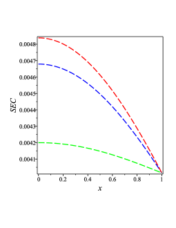
(e)  Strong energy condition

Figure 2: Plots of 1(a) gradients of density and pressure, 1(b) speed of sound, 1(c) weak, 1(d) dominant and 1(e) strong energy conditions of model (II) , versus the dimensionless x using the constants constrained from Cen X-3.

Figure 2 1(a) illustrates that both the gradients of density and pressure are negative. Furthermore, Figure 2 1(b) demonstrates that the speed of sound is indeed less than unity, which is a necessary condition for a valid stellar model. Additionally, Figures 2 1(c), 1(d), and 1(e) exhibit the adherence to energy conditions. Hence, all the criteria associated with energy conditions are fulfilled within the model configuration of Cen X-3, thus meeting the requirements for a true, isotropic, and significant stellar model.

(a)  Equation of state $\omega=\frac{p(x)}{\rho(x)}$

(b)  The pressure as function of density i.e., $p(\rho)$

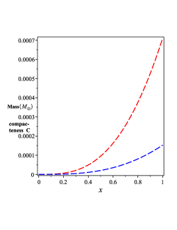
(c)  The mass and compactness of model (II)

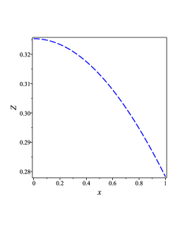
(d)  The red shift of the model (II)

Figure 3: Plot of 2(a) the EoS $\omega=\frac{p(x)}{\rho(x)}$ versus the dimensionless x using sing the constants constrained from Sen X-3, 2(b) the behavior of the pressure as a function of the energy-density, 2(c) the behavior of the mass and compactness and 2(d) shows the behavior of the red shift.

In Fig. 3 2(a) we depict the EoS against the dimensionless $x$ which shows a nonlinear behavior. In Fig. 3 2(b) we plot the pressure as a function of density which also shows a nonlinear behavior due to the isotropy of model (II). As Figs. 3 2(a) and 3 2(b) indicate that the source of the non-linearity of the EOS is not the mimetic scalar field only but also the isotropy of the stellar model under consideration.

The mass function given by Eq. (12) is depicted in Fig 3 2(c). Fig. 3 2(c) show that the behavior of the mass and compactness are monotonically increasing of $x$ and $M_{{}_{x=0}}=0$. Moreover, Fig. 3 2(c) show the behavior of the compactness parameter of stellar which are also increasing. Fig. 3 2(c) shows that the maximum value of the compactness of the Cen X-3 is $0.00015$ as shown which is smaller than the value of GR which is $0.2035$ Torres-Sánchez and Contreras (2019). Finally, Fig. 3 2(d) indicates the behavior of the red shift of the stellar. Böhmer and Harko Böhmer and Harko (2006) limited the boundary red-shift to be $Z\leq 5$. The boundary redshift of the model under consideration is evaluated and get $0.278269891$.

V Stability of the model

We will examine the matter of stability through the utilization of two approaches: the Tolman-Oppenheimer-Volkoff (TOV) equations and the adiabatic index.

V.1 Equilibrium using Tolman-Oppenheimer-Volkoff equation

Now, we discuss the stability of the model (II) by supposing hydrostatic equilibrium through the TOV equation. TOV equation Tolman (1939); Oppenheimer and Volkoff (1939) as presented in Ponce de Leon (1993), gives the following form of an isotropic model:

$$-\frac{M_{g}(x)[\rho(x)+p(x)]{E}}{x\sqrt{E_{1}}}-\frac{dp}{dx}=0,$$ (27)

where $M_{g}(x)$ is the gravitational mass which is given by:

$$M_{g}(x)=4\pi{\int_{0}}^{x}\Big{(}{T_{t}}^{t}-{T_{r}}^{r}-{T_{\theta}}^{\theta}-{T_{\phi}}^{\phi}\Big{)}\eta^{2}E\sqrt{E_{1}}d\eta=\frac{xE^{\prime}\sqrt{E_{1}}}{2E^{2}}\,,$$ (28)

Inserting Eq. (28) into (27), we get

$$-\frac{dp}{dx}-\frac{E^{\prime}[\rho(x)+p(x)]}{2E}=F_{g}+F_{h}=0\,,$$ (29)

with $F_{g}=-\frac{E^{\prime}[\rho(x)+p(x)]}{2{E}}$ and $F_{h}=-\frac{dp(x)}{dx}$ are the gravitational and the hydrostatic forces respectively.

These two different forces,are plotted in Fig. 4. Therefore, we prove that the pulsar in static equilibrium is stable through the TOV equation.

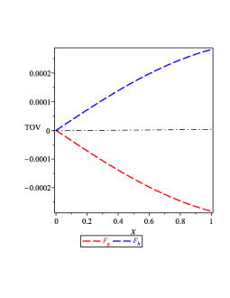
(a)  TOV equation

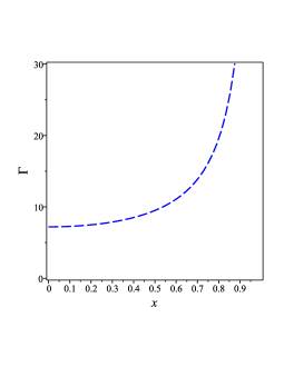
(b)  Adiabatic index

Figure 4: Plots of 3(a) the TOV equation 3(b) the adiabatic index versus the dimensionless $x$.

V.2 Adiabatic index

Another way to examine the stability of the model under consideration is to study the stability configuration using the adiabatic index that is considered an essential test. The adiabatic index $\Gamma$ is given by: Chandrasekhar (1964); Merafina and Ruffini (1989); Chan et al. (1993)

$$\Gamma=\left(\frac{\rho(x)+p(x)}{p(x)}\right)\left(\frac{dp(x)}{d\rho(x)}\right)\,.$$ (30)

To have stability equilibrium the adiabatic index $\Gamma$ must be $\Gamma>\frac{4}{3}$ Heintzmann and Hillebrandt (1975). For $\Gamma=\frac{4}{3}$, the isotropic sphere possesses a neutral equilibrium. From Eq. (30), we obtain the adiabatic index of the model (II) as:

$$\Gamma=\frac{3\left(1+u{x}^{2}\right)\left(3+u{x}^{2}\right)\varepsilon}{\left(5+u{x}^{2}\right)^{2}}\left\{\left(12{u}^{2}{x}^{4}+15u{x}^{2}+5\right)(4u\varepsilon+w)\left(1+u{x}^{2}\right)^{2}\varepsilon+\biggl{(}72{u}^{3}{x}^{6}+190\,{u}^{2}{x}^{4}+167u{x}^{2}+50\biggr{)}\varepsilon^{2}u\right\}^{-1}$$

$$\bigg{\{}(w-4u\varepsilon_{1})\left(1+u{x}^{2}\right)\left(24{u}^{3}{x}^{6}+70{u}^{2}{x}^{4}+75u{x}^{2}+50\right)+\varepsilon u\left(16{u}^{3}{x}^{6}+28{u}^{2}{x}^{4}+40u{x}^{2}+25\right)\bigg{\}}^{2}\biggl{\{}3(w-4u\varepsilon_{1})\left(1+u{x}^{2}\right)$$

$$\times\left(16{u}^{4}{x}^{8}+88{u}^{3}{x}^{6}+166{u}^{2}{x}^{4}+115u{x}^{2}+25\right)+u\varepsilon\biggl{(}372{u}^{2}{x}^{4}+32{u}^{4}{x}^{8}+96{u}^{3}{x}^{6}+480u{x}^{2}+175\biggr{)}\biggr{\}}^{-1}\,.$$ (31)

Figure 4 3(b) displays the parameter $\Gamma$, indicating that its values surpass the threshold of $4/3$ within the interior model. This observation confirms that the stability condition is met, as required.

Table 1: Values of model parameters

Star	Reference.	Mass	radius [km]	$a_{0}$	$u$	$w$
Her X-1	Abubekerov et al. (2008)	$0.85\pm 0.15$	$8.1\pm 0.41$	$-0.1738264671$	$0.1453714459$	$-2.764746699$
Cen X-3	Naik et al. (2011)	$1.49\pm 0.49$	$9.178\pm 0.13$	$-0.1509026812$	$0.1241376545$	$-2.382227207$
RX J185635-3754	Pons et al. (2002)	$0.9\pm 0.2$	$\simeq 6$	$-0.1583616821$	$0.1300851651$	$-2.489973265$
4U1608 - 52	Marshall and Angelini (1996)	$1.57\pm 0.3$	$9.8\pm 1.8$	$-0.1637386840$	$0.1349013201$	$-2.576874315$
EXO 1745-268	Ozel et al. (2009)	$1.65\pm 0.25$	$10.5\pm 1.8$	$-0.1653378835$	$0.1364292317$	$-2.604379240$
4U 1820-30	Güver et al. (2010)	$1.46\pm 0.2$	$11.1\pm 1.8$	$-0.1713098595$	$0.1425649058$	$-2.714525397$

Table 2: Values of physical quantities

Pulsar	$\rho\lvert_{{}_{{}_{x\rightarrow 0}}}$	$\rho\lvert_{{}_{{}_{x\rightarrow 1}}}$	$\frac{dp}{d\rho}\lvert_{{}_{{}_{x\rightarrow 0}}}$	$\frac{dp}{d\rho}\lvert_{{}_{{}_{x\rightarrow 1}}}$	$(\rho-3p_{r})\lvert_{{}_{{}_{x\rightarrow 0}}}$	$(\rho-3p)\lvert_{{}_{{}_{x\rightarrow 1}}}$	$z\lvert_{{}_{{}_{x\rightarrow 1}}}$
	[$g/cm^{3}$]	[$g/cm^{3}$]			[$Pa$]	[$Pa$]
Her X-1	$\thickapprox$0.0064	$\thickapprox$0.0054	$\thickapprox$0.24	$\thickapprox$0.25	$\thickapprox$0.0057	$\thickapprox$0.0054	0.1
Cen X-3	$\thickapprox$0.0047	$\thickapprox$0.004	$\thickapprox$0.238	$\thickapprox$0.246	$\thickapprox$0.0042	$\thickapprox$0.004	0.28
RX J 1856 -3754	$\thickapprox$0.011	$\thickapprox$0.01	$\thickapprox$0.238	$\thickapprox$0.246	$\thickapprox$0.011	$\thickapprox$0.01	0.22
4U1608 - 52	$\thickapprox$0.003	$\thickapprox$0.002	$\thickapprox$0.238	$\thickapprox$0.247	$\thickapprox$0.0029	$\thickapprox$0.0028	0.18
EXO 1785 - 248	$\thickapprox$0.0029	$\thickapprox$0.0025	$\thickapprox$0.238	$\thickapprox$0.247	$\thickapprox$0.0026	$\thickapprox$0.0025	0.16
4U1820 - 30	$\thickapprox$0.0028	$\thickapprox$0.0023	$\thickapprox$0.238	$\thickapprox$0.248	$\thickapprox$0.0024	$\thickapprox$0.0023	0.12

In addition to the pulsar known as Cen X-3, a comparable analysis can be conducted for other pulsars as well. We present concise outcomes for the remaining observed pulsars in Tables I and II.

VI Discussion and conclusions

In the present study, we have derived isotropic model of mimetic gravitational theory, for the first time, without assuming any specific form of the EoS. The construction of such model based on the assumption of the metric potential’s temporal component and the vanishing of the anisotropy. The main feature of this model was its dependence on three dimensionless constants which we fixed them through the matching condition with the exterior vacuum solution of this theory, i.e., the Schwarzschild solution Nashed et al. (2019), and the vanishing of the pressure on the surface of the stellar. The physical tests carried out can be summarized: a-The density and pressure must be finite at the center of the stellar configuration, and the pressure must be zero at the surface of the star, Figs. 1 0(a) and 1 0(b).
b-The negative values of the gradients of density and pressure Fig. 2 1(a), the validation of the causality Fig. 2 1(b) as well as its verification of the energy conditions, Figs. 2 1(c), 1(d) and 1(e).
c-Moreover, we have shown that the EoS parameter, $\omega=\frac{p(x)}{\rho(c)}$ as well as EoS, $p(\rho)=\omega\rho$, behave in a non-linear form which is a feature of the isotropic model, Figs. 3 2(a) and 3 2(b). Furthermore, we have shown the behavior of the mass and compactness are increasing, and the red-shift of this model has a value on the star’s surface as $Z=0.2782$ as shown in Figs. 3 2(c) and 3 2(d).
d-One of the merits of this model is that it verified the TOV equation as shown in Fig. 4 3(a) and its behavior of the adiabatic index is shown in Fig. 4 3(b).

Additionally, we have examined our model with other six pulsars and derived the numerical values of their constants. Finally, we have derived the numerical values of the density at the center and at the star’s surface, the EoS parameter, $\omega$, at the center and the surface of the start, the strong energy condition, and the red-shift at the surface of the stellar configuration. In tables I and II, we tabulated all those data.

To conclude, as far as we know, this is the first time to derive an isotropic model in the framework of the mimetic gravitational theory without assuming any specific form of the EoS. Can this procedure be applied to any other modified gravitational theory like $f(R)$ or $f(T)$? This task will be our coming study.

Data Availability Statement

No Data associated in the manuscript.

Ethics declarations

Conflict of interest The author declares that there is no conflict of interests regarding the publication of this paper.

References

- Carroll et al. (2004) S. Carroll, S. Carroll, and Addison-Wesley, Spacetime and Geometry: An Introduction to General Relativity (Addison Wesley, 2004).
- Will (2006) C. M. Will, Living Rev. Rel. 9, 3 (2006), arXiv:gr-qc/0510072 .
- Abbott et al. (2016) B. P. Abbott et al. (LIGO Scientific, Virgo), Phys. Rev. Lett. 116, 061102 (2016), arXiv:1602.03837 [gr-qc] .
- Chamseddine and Mukhanov (2013) A. H. Chamseddine and V. Mukhanov, JHEP 11, 135 (2013), arXiv:1308.5410 [astro-ph.CO] .
- Deruelle and Rua (2014) N. Deruelle and J. Rua, JCAP 09, 002 (2014), arXiv:1407.0825 [gr-qc] .
- Domènech et al. (2015) G. Domènech, S. Mukohyama, R. Namba, A. Naruko, R. Saitou, and Y. Watanabe, Phys. Rev. D 92, 084027 (2015), arXiv:1507.05390 [hep-th] .
- Firouzjahi et al. (2018) H. Firouzjahi, M. A. Gorji, S. A. Hosseini Mansoori, A. Karami, and T. Rostami, JCAP 11, 046 (2018), arXiv:1806.11472 [gr-qc] .
- Shen et al. (2019) L. Shen, Y. Zheng, and M. Li, JCAP 12, 026 (2019), arXiv:1909.01248 [gr-qc] .
- Chamseddine and Mukhanov (2017a) A. H. Chamseddine and V. Mukhanov, JCAP 03, 009 (2017a), arXiv:1612.05860 [gr-qc] .
- Chamseddine and Mukhanov (2017b) A. H. Chamseddine and V. Mukhanov, Eur. Phys. J. C 77, 183 (2017b), arXiv:1612.05861 [gr-qc] .
- Casalino et al. (2018) A. Casalino, M. Rinaldi, L. Sebastiani, and S. Vagnozzi, Phys. Dark Univ. 22, 108 (2018), arXiv:1803.02620 [gr-qc] .
- Casalino et al. (2019) A. Casalino, M. Rinaldi, L. Sebastiani, and S. Vagnozzi, Class. Quant. Grav. 36, 017001 (2019), arXiv:1811.06830 [gr-qc] .
- Sherafati et al. (2021) K. Sherafati, S. Heydari, and K. Karami, (2021), arXiv:2109.11810 [gr-qc] .
- Vagnozzi (2017) S. Vagnozzi, Class. Quant. Grav. 34, 185006 (2017), arXiv:1708.00603 [gr-qc] .
- Sheykhi and Grunau (2021) A. Sheykhi and S. Grunau, Int. J. Mod. Phys. A 36, 2150186 (2021), arXiv:1911.13072 [gr-qc] .
- Chamseddine et al. (2014) A. H. Chamseddine, V. Mukhanov, and A. Vikman, JCAP 06, 017 (2014), arXiv:1403.3961 [astro-ph.CO] .
- Baffou et al. (2017) E. H. Baffou, M. J. S. Houndjo, M. Hamani-Daouda, and F. G. Alvarenga, Eur. Phys. J. C 77, 708 (2017), arXiv:1706.08842 [gr-qc] .
- Dutta et al. (2018) J. Dutta, W. Khyllep, E. N. Saridakis, N. Tamanini, and S. Vagnozzi, JCAP 02, 041 (2018), arXiv:1711.07290 [gr-qc] .
- Sheykhi (2018) A. Sheykhi, Int. J. Mod. Phys. D 28, 1950057 (2018).
- Abbassi et al. (2018) M. H. Abbassi, A. Jozani, and H. R. Sepangi, Phys. Rev. D 97, 123510 (2018), arXiv:1803.00209 [gr-qc] .
- Matsumoto (2016) J. Matsumoto, (2016), arXiv:1610.07847 [astro-ph.CO] .
- Sebastiani et al. (2017) L. Sebastiani, S. Vagnozzi, and R. Myrzakulov, Adv. High Energy Phys. 2017, 3156915 (2017), arXiv:1612.08661 [gr-qc] .
- Sadeghnezhad and Nozari (2017) N. Sadeghnezhad and K. Nozari, Phys. Lett. B 769, 134 (2017), arXiv:1703.06269 [gr-qc] .
- Gorji et al. (2019) M. A. Gorji, S. Mukohyama, and H. Firouzjahi, JCAP 05, 019 (2019), arXiv:1903.04845 [gr-qc] .
- Gorji et al. (2018a) M. A. Gorji, S. Mukohyama, H. Firouzjahi, and S. A. Hosseini Mansoori, JCAP 08, 047 (2018a), arXiv:1807.06335 [hep-th] .
- Bouhmadi-López et al. (2017) M. Bouhmadi-López, C.-Y. Chen, and P. Chen, JCAP 11, 053 (2017), arXiv:1709.09192 [gr-qc] .
- Gorji et al. (2018b) M. A. Gorji, S. A. Hosseini Mansoori, and H. Firouzjahi, JCAP 01, 020 (2018b), arXiv:1709.09988 [astro-ph.CO] .
- Chamseddine et al. (2019a) A. H. Chamseddine, V. Mukhanov, and T. B. Russ, Eur. Phys. J. C 79, 558 (2019a), arXiv:1905.01343 [hep-th] .
- Russ (2021) T. B. Russ, (2021), arXiv:2103.12442 [gr-qc] .
- de Cesare et al. (2020) M. de Cesare, S. S. Seahra, and E. Wilson-Ewing, JCAP 07, 018 (2020), arXiv:2002.11658 [gr-qc] .
- Farsi and Sheykhi (2022) B. Farsi and A. Sheykhi, (2022), arXiv:2202.04118 [gr-qc] .
- Cárdenas et al. (2021) V. H. Cárdenas, M. Cruz, S. Lepe, and P. Salgado, Phys. Dark Univ. 31, 100775 (2021), arXiv:2009.03203 [gr-qc] .
- Hosseini Mansoori et al. (2021) S. A. Hosseini Mansoori, A. Talebian, and H. Firouzjahi, JHEP 01, 183 (2021), arXiv:2010.13495 [gr-qc] .
- Arroja et al. (2018) F. Arroja, T. Okumura, N. Bartolo, P. Karmakar, and S. Matarrese, JCAP 05, 050 (2018), arXiv:1708.01850 [astro-ph.CO] .
- Gorji et al. (2020) M. A. Gorji, A. Allahyari, M. Khodadi, and H. Firouzjahi, Phys. Rev. D 101, 124060 (2020), arXiv:1912.04636 [gr-qc] .
- Myrzakulov and Sebastiani (2015) R. Myrzakulov and L. Sebastiani, Gen. Rel. Grav. 47, 89 (2015), arXiv:1503.04293 [gr-qc] .
- Nashed and El Hanafy (2017) G. G. L. Nashed and W. El Hanafy, Eur. Phys. J. , 90 (2017), arXiv:1612.05106 [gr-qc] .
- Nashed (2011) G. G. L. Nashed, Annalen Phys. 523, 450 (2011), arXiv:1105.0328 [gr-qc] .
- Myrzakulov et al. (2016) R. Myrzakulov, L. Sebastiani, S. Vagnozzi, and S. Zerbini, Class. Quant. Grav. 33, 125005 (2016), arXiv:1510.02284 [gr-qc] .
- Ganz et al. (2019) A. Ganz, P. Karmakar, S. Matarrese, and D. Sorokin, Phys. Rev. D 99, 064009 (2019), arXiv:1812.02667 [gr-qc] .
- Chen et al. (2018) C.-Y. Chen, M. Bouhmadi-López, and P. Chen, Eur. Phys. J. C 78, 59 (2018), arXiv:1710.10638 [gr-qc] .
- Nashed (2018a) G. G. L. Nashed, Int. J. Geom. Meth. Mod. Phys. 15, 1850154 (2018a).
- Ben Achour et al. (2018) J. Ben Achour, F. Lamy, H. Liu, and K. Noui, JCAP 05, 072 (2018), arXiv:1712.03876 [gr-qc] .
- Brahma et al. (2018) S. Brahma, A. Golovnev, and D.-H. Yeom, Phys. Lett. B 782, 280 (2018), arXiv:1803.03955 [gr-qc] .
- Zheng et al. (2017) Y. Zheng, L. Shen, Y. Mou, and M. Li, JCAP 08, 040 (2017), arXiv:1704.06834 [gr-qc] .
- Nashed et al. (2019) G. G. L. Nashed, W. El Hanafy, and K. Bamba, JCAP 01, 058 (2019), arXiv:1809.02289 [gr-qc] .
- Chamseddine et al. (2019b) A. H. Chamseddine, V. Mukhanov, and T. B. Russ, JHEP 10, 104 (2019b), arXiv:1908.03498 [hep-th] .
- Sheykhi (2020) A. Sheykhi, JHEP 07, 031 (2020), arXiv:2002.11718 [gr-qc] .
- Sheykhi (2021) A. Sheykhi, JHEP 01, 043 (2021), arXiv:2009.12826 [gr-qc] .
- Nashed and Nojiri (2021) G. G. L. Nashed and S. Nojiri, Phys. Rev. D 104, 044043 (2021), arXiv:2107.13550 [gr-qc] .
- Chamseddine (2021) A. H. Chamseddine, Eur. Phys. J. C 81, 977 (2021), arXiv:2106.14235 [hep-th] .
- Bakhtiarizadeh (2021) H. R. Bakhtiarizadeh, (2021), arXiv:2107.10686 [gr-qc] .
- Nashed (2021) G. G. L. Nashed, Astrophys. J. 919, 113 (2021), arXiv:2108.04060 [gr-qc] .
- Nojiri and Odintsov (2014) S. Nojiri and S. D. Odintsov, (2014), 10.1142/S0217732314502113, [Erratum: Mod.Phys.Lett.A 29, 1450211 (2014)], arXiv:1408.3561 [hep-th] .
- Odintsov and Oikonomou (2016a) S. D. Odintsov and V. K. Oikonomou, Phys. Rev. D 93, 023517 (2016a), arXiv:1511.04559 [gr-qc] .
- Oikonomou (2016a) V. K. Oikonomou, Mod. Phys. Lett. A 31, 1650191 (2016a), arXiv:1609.03156 [gr-qc] .
- Oikonomou (2016b) V. K. Oikonomou, Int. J. Mod. Phys. D 25, 1650078 (2016b), arXiv:1605.00583 [gr-qc] .
- Oikonomou (2016c) V. K. Oikonomou, Universe 2, 10 (2016c), arXiv:1511.09117 [gr-qc] .
- Myrzakulov and Sebastiani (2016) R. Myrzakulov and L. Sebastiani, Astrophys. Space Sci. 361, 188 (2016), arXiv:1601.04994 [gr-qc] .
- Odintsov and Oikonomou (2015) S. D. Odintsov and V. K. Oikonomou, Annals Phys. 363, 503 (2015), arXiv:1508.07488 [gr-qc] .
- Odintsov and Oikonomou (2016b) S. D. Odintsov and V. K. Oikonomou, Astrophys. Space Sci. 361, 236 (2016b), arXiv:1602.05645 [gr-qc] .
- Odintsov and Oikonomou (2016c) S. D. Odintsov and V. K. Oikonomou, Phys. Rev. D 94, 044012 (2016c), arXiv:1608.00165 [gr-qc] .
- Nojiri et al. (2017a) S. Nojiri, S. D. Odintsov, and V. K. Oikonomou, Phys. Lett. B 775, 44 (2017a), arXiv:1710.07838 [gr-qc] .
- Odintsov and Oikonomou (2018) S. D. Odintsov and V. K. Oikonomou, Nucl. Phys. B 929, 79 (2018), arXiv:1801.10529 [gr-qc] .
- Bhattacharjee (2021) S. Bhattacharjee, (2021), arXiv:2104.01751 [gr-qc] .
- Kaczmarek and Szczesniak (2021) A. Z. Kaczmarek and D. Szczesniak, Sci. Rep. 11, 18363 (2021), arXiv:2105.05050 [gr-qc] .
- Chen et al. (2021) J. Chen, W.-D. Guo, and Y.-X. Liu, Eur. Phys. J. C 81, 709 (2021), arXiv:2011.03927 [gr-qc] .
- Astashenok et al. (2015) A. V. Astashenok, S. D. Odintsov, and V. K. Oikonomou, Class. Quant. Grav. 32, 185007 (2015), arXiv:1504.04861 [gr-qc] .
- Oikonomou (2015) V. K. Oikonomou, Phys. Rev. D 92, 124027 (2015), arXiv:1509.05827 [gr-qc] .
- Zhong and Elizalde (2016) Y. Zhong and E. Elizalde, Mod. Phys. Lett. A 31, 1650221 (2016), arXiv:1612.04179 [gr-qc] .
- Zhong and Sáez-Chillón Gómez (2018) Y. Zhong and D. Sáez-Chillón Gómez, Symmetry 10, 170 (2018), arXiv:1805.03467 [gr-qc] .
- Paul et al. (2020) B. C. Paul, S. D. Maharaj, and A. Beesham, (2020), arXiv:2008.00169 [astro-ph.CO] .
- Nojiri et al. (2016) S. Nojiri, S. D. Odintsov, and V. K. Oikonomou, Phys. Rev. D 94, 104050 (2016), arXiv:1608.07806 [gr-qc] .
- Saadi (2016) H. Saadi, Eur. Phys. J. C 76, 14 (2016), arXiv:1411.4531 [gr-qc] .
- Haghani et al. (2015) Z. Haghani, T. Harko, H. R. Sepangi, and S. Shahidi, JCAP 05, 022 (2015), arXiv:1501.00819 [gr-qc] .
- Addazi and Marciano (2017) A. Addazi and A. Marciano, Symmetry 9, 249 (2017), arXiv:1710.07962 [gr-qc] .
- Astashenok and Odintsov (2016) A. V. Astashenok and S. D. Odintsov, Phys. Rev. D 94, 063008 (2016), arXiv:1512.07279 [gr-qc] .
- Babichev and Ramazanov (2017) E. Babichev and S. Ramazanov, Phys. Rev. D 95, 024025 (2017), arXiv:1609.08580 [gr-qc] .
- Nashed (2018b) G. Nashed, Symmetry 10, 559 (2018b).
- Nashed et al. (2020) G. G. L. Nashed, A. Abebe, and K. Bamba, Eur. Phys. J. C 80, 1109 (2020).
- Nashed and Capozziello (2020) G. G. L. Nashed and S. Capozziello, Eur. Phys. J. C 80, 969 (2020), arXiv:2010.06355 [gr-qc] .
- Torres-Sánchez and Contreras (2019) V. A. Torres-Sánchez and E. Contreras, Eur. Phys. J. C 79, 829 (2019), arXiv:1908.08194 [gr-qc] .
- Estevez-Delgado et al. (2019) G. Estevez-Delgado, J. Estevez-Delgado, N. M. García, and M. P. Duran, Can. J. Phys. 97, 988 (2019), arXiv:1807.10360 [gr-qc] .
- Newton Singh et al. (2019) K. Newton Singh, F. Rahaman, and A. Banerjee, Phys. Rev. D 100, 084023 (2019), arXiv:1909.10882 [gr-qc] .
- Roupas and Nashed (2020) Z. Roupas and G. G. L. Nashed, Eur. Phys. J. C 80, 905 (2020), arXiv:2007.09797 [gr-qc] .
- Zeldovich and Novikov (1971) Y. B. Zeldovich and I. D. Novikov, Relativistic astrophysics. Vol.1: Stars and relativity (1971).
- Shirafuji et al. (1996) T. Shirafuji, G. G. L. Nashed, and K. Hayashi, Prog. Theor. Phys. 95, 665 (1996), arXiv:gr-qc/9601044 .
- Gangopadhyay et al. (2013) T. Gangopadhyay, S. Ray, X.-D. Li, J. Dey, and M. Dey, Mon. Not. Roy. Astron. Soc. 431, 3216 (2013), arXiv:1303.1956 [astro-ph.HE] .
- Naik et al. (2011) S. Naik, B. Paul, and Z. Ali, Astrophys. J. 737, 79 (2011), arXiv:1106.0370 [astro-ph.SR] .
- Böhmer and Harko (2006) C. G. Böhmer and T. Harko, Classical and Quantum Gravity 23, 6479 (2006).
- Tolman (1939) R. C. Tolman, Phys. Rev. 55, 364 (1939).
- Oppenheimer and Volkoff (1939) J. R. Oppenheimer and G. M. Volkoff, Phys. Rev. 55, 374 (1939).
- Ponce de Leon (1993) J. Ponce de Leon, General Relativity and Gravitation 25, 1123 (1993).
- Chandrasekhar (1964) S. Chandrasekhar, Astrophys. J. 140, 417 (1964).
- Merafina and Ruffini (1989) M. Merafina and R. Ruffini, aap 221, 4 (1989).
- Chan et al. (1993) R. Chan, L. Herrera, and N. O. Santos, Monthly Notices of the Royal Astronomical Society 265, 533 (1993), http://oup.prod.sis.lan/mnras/article-pdf/265/3/533/3807712/mnras265-0533.pdf .
- Heintzmann and Hillebrandt (1975) H. Heintzmann and W. Hillebrandt, aap 38, 51 (1975).
- Abubekerov et al. (2008) M. K. Abubekerov, E. A. Antokhina, A. M. Cherepashchuk, and V. V. Shimanskii, Astronomy Reports 52, 379 (2008).
- Pons et al. (2002) J. A. Pons, F. M. Walter, J. M. Lattimer, M. Prakash, R. Neuhäuser, and P. An, Astrophys. J. 564, 981 (2002), arXiv:astro-ph/0107404 [astro-ph] .
- Marshall and Angelini (1996) F. E. Marshall and L. Angelini, IAU Circ. 6331, 1 (1996).
- Ozel et al. (2009) F. Ozel, T. Guver, and D. Psaltis, Astrophys. J. 693, 1775 (2009), arXiv:0810.1521 [astro-ph] .
- Güver et al. (2010) T. Güver, P. Wroblewski, L. Camarota, and F. Özel, The Astrophysical Journal 719, 1807 (2010).