Dynamical structure factor and a new method to measure the pairing gap in two-dimensional attractive Fermi-Hubbard model

Abstract

By calculating the dynamical structure factor along the high symmetry directions in the Brillouin zone, the dynamical excitations in two-dimensional attractive Fermi-Hubbard model are studied based on the random-phase approximation. At the small transfer momentum, the sound speed can be obtained and is suppressed by the interaction strength. In particular, at the transfer momentum ${\bf q}=\left[\pi,\pi\right]$, the dynamical structure factor consists of a sharp bosonic molecular excitation peak in the low-energy region and a broad atomic excitation band in the higher energy region. Furthermore, as the hopping strength increases (the interaction strength decreases), the weight of the molecular excitation peak decreases monotonically while the weight of the atomic excitations increases quickly. The area of the molecular excitation peak scales with the square of the pairing gap, which also applies to the spin-orbit coupling case. These theoretical results show that the pairing gap in optical lattice can be obtained experimentally by measuring the dynamical structure factor at ${\bf q}=\left[\pi,\pi\right]$.

I Introduction

When quantum many-body Fermi atomic gas comes into the superfluid state, a non-zero paring gap (or order parameter) will be present. Finding a convenient way to measure the pairing gap is essential to understand many-body pairing phenomenon and dynamical excitations. Currently the pairing gap are mainly gained by all kinds of excited progresses, like momentum-resolved photo-emission spectroscopy Feld11 ; Stewart2008 , or radio-frequency spectroscopy Frohlich2011 ; Chin2004 ; Sommer2012 . However, it is difficult to measure the pairing gap well when the band structure becomes complex owing to the appearance of the magnetic fields or spin-orbit coupling (SOC) Zhai2015 ; Cheuk2012 ; Wang2012 ; Wang2021 ; Wu2013 ; Han2023 . Moreover, the dynamical excitations are also an important method to study pairing correlation information. We obtain the dynamical excitations by using the dynamical structure factor which is the Fourier transformation of the density-density correlation function. Therefore, the dynamical structure factor reflects the two-body correlation physics directly. The dynamical structure factor can be measured by two-photon Bragg scattering experiments according to measure the speed of center-of-mass of system Veeravalli08 ; Hoinka17 ; Biss2022 ; Senaratne2022 ; Li2022 ; Pagano2014 .

In the continuous Fermi gases, the collective excitations are studied at a small transferred momentum regime, while the single-particle excitations of the unpaired and paired atoms are usually shown at a large transferred momentum. Specifically the excitations of the paired atoms correspond to the bosonic molecular excitations. Experimentally C. J. Vale et al studied the single-particle excitations at a large transfer momentum $q{\gg}k_{F}$ with two-photon Bragg scattering technique, and found that the weight of the molecular scattering peak increases while the weight of the atomic scattering peak decreases during the BCS-BEC crossover Veeravalli08 . Later with the same technique, they investigated the Goldstone phonon mode and pair-breaking excitation by measuring the dynamical structure factor in the small transfer momentum region Hoinka17 , and found that the sound speed can be suppressed by the strong interaction. In 2022, H. Biss et al experimentally studied the phonon dispersion through the whole BCS-BEC crossover by using the Bragg scattering experiment Biss2022 . Moreover, theoretically the dynamical structure factors of three-dimensional (3D) Fermi gases had been studied well Combescot06 ; Combescot2006 ; Zou10 ; Zou16 ; Zou18 ; Hu18 ; Zou2021 ; Kuhnle10 ; Watabe10 . For two-dimensional (2D) superfluid Fermi gases, the Quantum Monte Carlo (QMC) method is developed to calculate the dynamical structure factor at a large transferred momentum, by which E. Vitali et al investigated the weight change of both the molecular excitations and atomic excitations Vitali17 . For other low-dimensional Fermi gases, several theoretical works had been carried out to study the dynamical excitation with dynamical structure factor Zhao2020 ; Gao2023 .

As to the discrete ultracold atomic gases, an optical lattice generated by superimposing orthogonal standing waves can be widely used to simulate the physics in solid Bloch2008 ; Wu2016 , and the system can be described by the Bose-Hubbard model or Fermi-Hubbard model Greiner2002 ; Spielman2008 ; Thomas2017 ; Jrdens08 ; Schneider08 ; Greif13 ; Hart15 ; Parsons16 ; Cheuk16 ; Koepsell2021 ; Boll16 ; Brown17 . Several theoretical groups had studied the attractive Fermi-Hubbard model, which is closely related to the strongly correlated systems in condensed matter physics Scalettar89 ; Kyung01 ; Honerkamp2004 ; Mondaini2015 ; Cocchi16 ; Strohmaier07 ; Ho04 ; Moreo07 ; Gukelberger16 ; Paiva04 ; Shenoy2008 . Experimentally the attractive Fermi-Hubbard model in cold atoms had been realized Mitra18 ; Hackermuller10 ; Peter20 ; Gall2020 ; Schneider12 . To date, there is no two-photon Bragg spectroscopy experiment on 2D Fermi gases in optical lattice. In 2020, E. Vitali et al numerically simulated the dynamical structure factor along the high symmetry directions in the Brillouin zone (BZ) of the attractive Fermi-Hubbard model on a square optical lattice at half-filling Vitali2020 , gave the low-energy Nambu-Goldstone collective mode and single-particle excitations in the higher energy region. However, there is no work to study the molecular scattering in this discrete system, which is closely related to the pairing gap. In this paper, we theoretically investigate dynamical excitations of 2D Fermi superfluid in optical lattice, and analyze their main characteristics in both collective and single-particle excitation. In general, the doping to the system can change the Fermi energy, then influence dynamical excitations. Therefore, we focus on the change of dynamical excitations from the half-filling to the doped cases. In particular, we will show that the molecular excitations can be displayed at the momentum ${\bf q}=\left[\pi,\pi\right]$, which provides a simple method to measure the pairing gap in doped system, which is due to that the square of the pairing gap is proportional to the area of the molecular excitation peak. Moreover, this method to measure pairing gap can be generalized to other Fermi atoms with SOC in optical lattice where the band structure becomes complex and the pairing gap is hard to detect directly Zhao2023 .

This paper is organized as follows. In the next section, we will use the language of Green’s function to solve the 2D Fermi-Hubbard model in mean field approximation, and self-consistently calculate the chemical potential and pairing gap. In Sec. III, we introduce how to calculate dynamical structure factor with random phase approximation (RPA). We display results of dynamic structure factor in the half-filling and compare with the QMC results in Sec. IV. In Sec. V, we calculate the dynamic structure factor when the system is away from the half-filling, and discuss the hopping dependence of the sound speed and the dynamical excitation at a certain transferred momentum ${\bf q}=\left[\pi,\pi\right]$. In Sec. VI, the dynamic structure factor varies with the further increase of doping. Finally we give our conclusions and acknowledgment. Some calculation details will be given in the appendix.

II Model and Hamiltonian

An attractive Fermi-Hubbard model can be used to describe a Fermi superfluid in 2D square optical lattices with a Hamiltonian in spatial representation described as follows:

$$H= - t\sum_{<ij>}C_{i\sigma}^{\dagger}C_{j\sigma}-\mu\sum_{i}C_{i\uparrow}^{\dagger}C_{i\sigma}$$ (1)

$$- U\sum_{i}C_{i\uparrow}^{\dagger}C_{i\downarrow}^{\dagger}C_{i\downarrow}C_{i\uparrow},$$

where $\left<ij\right>$ means the nearest-neighbor sites of lattice. $C_{i\sigma}^{\dagger}(C_{i\sigma})$ is the creation (annihilation) operator of a particle with spin $\sigma$ at site $i$, with hopping energy $t$ and chemical potential $\mu$. The Hubbard energy $U>0$ is the strength of on-site two-body attraction interaction, and set to be an energy unit in our following discussion. Also the lattice length $a_{0}=1$ used as unit of length. Within the mean field theory, the four-operators interaction Hamiltonian can be dealt into a two-operators one with the definition of pairing gap $\Delta=U\left<C_{i\downarrow}C_{i\uparrow}\right>$. Then the above Hamiltonian is treated into a mean field one, whose expression in momentum space reads

$$H_{\rm MF} = \sum_{{\bf k},\sigma}\xi_{\bf k}C^{\dagger}_{{\bf k}\sigma}C_{{\bf k}\sigma}$$ (2)

$$- \sum_{{\bf k}}(\Delta^{*}C_{{\bf k}\downarrow}C_{-{\bf k}\uparrow}+H.c.)+\frac{|\Delta|^{2}}{U},$$

where $\xi_{\bf k}=-Zt\gamma_{\bf k}-\mu$ and $\gamma_{\bf k}=\left(\cos{k_{x}}+\cos{k_{y}}\right)/2$. The nearest number $Z=4$ for 2D square lattice. We define the diagonal Green’s function $G({\bf k},\tau-\tau^{{}^{\prime}})=-\left\langle T_{\tau}C_{{\bf k}\sigma}(\tau)C^{\dagger}_{{\bf k}\sigma}(\tau^{{}^{\prime}})\right\rangle$ and off-diagonal one $\Gamma^{\dagger}({\bf k},\tau-\tau^{{}^{\prime}})=-\left\langle T_{\tau}C^{\dagger}_{-{\bf k}\uparrow}(\tau)C^{\dagger}_{{\bf k}\downarrow}(\tau^{{}^{\prime}})\right\rangle$, respectively. Their expressions in momentum and energy representation are given by

$$G(\bf{k},\omega) = \frac{1}{2}\left(\frac{1+{\xi}_{\bf{k}}/E_{\bf{k}}}{\omega-E_{\bf{k}}}+\frac{1-{\xi}_{\bf{k}}/E_{\bf{k}}}{\omega+E_{\bf{k}}}\right),$$ (3a)

$$\Gamma^{\dagger}\left(\bf{k},\omega\right) = \frac{\Delta^{*}}{2E_{\bf{k}}}\left(\frac{1}{\omega-E_{\bf{k}}}-\frac{1}{\omega+E_{\bf{k}}}\right),$$ (3b)

where $E_{\bf{k}}=\sqrt{{\xi}^{2}_{\bf{k}}+{|\Delta|^{2}}}$ is the quasiparticle spectrum. The chemical potential $\mu$ and pairing gap $\Delta$ are determined by self-consistently solving the density of particle number equation and pairing gap equation

$$n = \frac{1}{2}\sum_{{\bf k}}\left(1-\frac{{\xi}_{\bf{k}}}{E_{\bf{k}}}\right){\rm tanh}\left(\frac{E_{\bf{k}}}{2T}\right),$$ (4)

$$1 = \frac{U}{N}\sum_{{\bf k}}\frac{1}{2E_{{\bf k}}}{\rm tanh}\left(\frac{E_{{\bf k}}}{2T}\right),$$ (5)

where Boltzmann constant $k_{B}=1$ here and in the following.

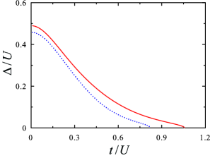
Figure 1: Pairing gap $\Delta$ as a function of $t$ for $n=0.8$ (red solid line) and $n=0.6$ (blue dotted line).

Close to zero temperature $T=0$, the pairing gap $\Delta$ can be chosen to be a real number in the ground state. Generally increasing hopping energy $t$ will decrease the value of pairing gas $\Delta$, and the relation between them at $n=0.8$ (red solid line) and $n=0.6$ (blue dotted line) is shown in Fig. 1. And pairing gas $\Delta=0$ at a large enough hopping energy $t$, which means that a phase transition from the superfluid state to the normal state happens. Moreover, $\Delta$ is clearly suppressed as particle density $n$ decreases.

III Dynamical structure factor and random phase approximation

In superfluid state, there are four different density. Besides the normal spin-up $\hat{n}_{1}=\left<C^{\dagger}_{i\uparrow}C_{i\uparrow}\right>$ and spin-down density $\hat{n}_{2}=\left<C^{\dagger}_{i\downarrow}C_{i\downarrow}\right>$, the anomalous density $\hat{n}_{3}=\left<C_{i\downarrow}C_{i\uparrow}\right>$ and its complex conjugate $\hat{n}_{4}=\left<C^{\dagger}_{i\uparrow}C^{\dagger}_{i\downarrow}\right>$ are important to describing Cooper pairing. These four densities are coupled with each other due to a non-zero interaction, and any perturbation in one density will induce density fluctuation in other densities. In the frame of linear response theory, the small external perturbation potential $V_{\rm ext}$ and density fluctuations $\delta n$ are connected with each other by response function of the system $\chi$, namely $\delta n=\chi V_{\rm ext}$. The mean-field theory fails to treat the contribution from the fluctuation term of interaction Hamiltonian, and can not give a well description about the dynamical excitations of an interacting system. In order to take fluctuation part back Liu2004 ; Zhao2020 ; Gao2023 , the random phase approximation (RPA) has been verified to be a good method to calculate response function $\chi$ beyond the mean-field theory. Based on this theory, the response function $\chi$ with fluctuation correction can be obtained can treating fluctuation Hamiltonian as part of an effective external potential, and finally find its connection to the mean-field response function $\chi^{0}$, which is shown by

$$\chi({\bf q},i\omega_{n})=\frac{\chi^{0}({\bf q},i\omega_{n})}{\hat{1}+\chi^{0}({\bf q},i\omega_{n})UG},$$ (6)

where $G=\sigma_{0}\otimes\sigma_{x}$ is a direct product of two Pauli matrices $\sigma_{0}$ and $\sigma_{x}$, $\sigma_{0}$ is the unit matrix and the unit matrix $\hat{1}=\sigma_{0}\otimes\sigma_{0}$.

The numerical calculation of mean-field response function $\chi^{0}$ is very easy, and its expression is given by the following matrix

$$\chi^{0}({\bf q},i\omega_{n})=\left[\begin{array}[]{cccccc}&\chi^{0}_{11}&\chi^{0}_{12}&\chi^{0}_{13}&\chi^{0}_{14}\\ &\chi^{0}_{21}&\chi^{0}_{22}&\chi^{0}_{23}&\chi^{0}_{24}\\ &\chi^{0}_{31}&\chi^{0}_{32}&\chi^{0}_{33}&\chi^{0}_{34}\\ &\chi^{0}_{41}&\chi^{0}_{42}&\chi^{0}_{43}&\chi^{0}_{44}\\ \end{array}\right].$$ (11)

The dimension of $\chi^{0}$ reflect the coupling situation in four different densities. These 16 matrix elements are determined by the corresponding density-density correlation functions which can be obtained by defining corresponding Green’s functions. In fact, as a result of the symmetry of system, only 6 of them are independent, i.e., $\chi^{0}_{11}=\chi^{0}_{22}$, $\chi^{0}_{12}=\chi^{0}_{21}=-\chi^{0}_{33}=-\chi^{0}_{44}$, $\chi^{0}_{31}=\chi^{0}_{32}=\chi^{0}_{14}=\chi^{0}_{24}$, $\chi^{0}_{41}=\chi^{0}_{42}=\chi^{0}_{13}=\chi^{0}_{23}$. Their expressions are listed in the final appendix of this paper.

The total density response function $\chi_{n}$ is defined by $\chi_{n}\equiv\chi_{11}+\chi_{12}+\chi_{21}+\chi_{22}$, its expression is given by

$$\chi_{n}({\bf q},i\omega_{n}) = \frac{2\chi_{1}}{\chi_{2}+U\chi_{1}},$$ (12)

where

$$\chi_{1} = \left|\begin{array}[]{cccc}&\chi^{0}_{11}+\chi^{0}_{12}&2\chi^{0}_{14}U&2\chi^{0}_{13}U\\ &\chi^{0}_{14}&1+\chi^{0}_{34}U&-\chi^{0}_{12}U\\ &\chi^{0}_{13}&-\chi^{0}_{12}U&1+\chi^{0}_{43}U\\ \end{array}\right|$$ (13d)

$$\chi_{2} = \left|\begin{array}[]{ccc}&1+\chi^{0}_{34}U&-\chi^{0}_{12}U\\ &-\chi^{0}_{12}U&1+\chi^{0}_{43}U\\ \end{array}\right|$$ (13g)

According to the fluctuation-dissipation theory, the density dynamical structure factor $S({\bf q},{\omega})$ is connected to the imaginary part of the density response function $\chi_{n}$ by

$$S({\bf q},{\omega}) = -\frac{1}{\pi}{\rm Im}\chi_{n}\left({\bf q},i\omega_{n}\to\omega+i\delta\right),$$ (14)

where ${\bf q}$ and $\omega$ are respectively the transferred momentum and energy. $\delta$ is a small positive number in numerical calculation (usually we set $\delta=0.003$).

IV Dynamical structure factor at half-filling $<n>=1$

Now we are ready to discuss the dynamical structure factor of 2D attractive Fermi-Hubbard model. By analyzing the density dynamical structure factor under different transfer momenta, one can obtain collective excitations and single-particle excitations of Fermi atoms in a 2D square optical lattice. We have calculated the energy and momentum dependence of density dynamical structure factor $S({\bf q},{\omega})$, and the contour plot of $S({\bf q},{\omega})$ along the high symmetry directions in the BZ for hopping strength (a) $t/U=0.25$, (b) $t/U=0.4$ at the half-filling $<n>=1$ are plotted in Fig. 2.

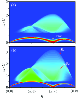
Figure 2: The color maps of the dynamical structure factor $S({\bf q},{\omega})$ as functions of transferred energy and momentum along the high-symmetry directions for hopping (a) $t/U=0.25$, (b) $t/U=0.4$ at the half-filling $<n>=1$. The red dashed line marks the dispersion of $E_{\rm d}$.

In the low-energy region, the collective mode is displayed by the $S({\bf q},{\omega})$ with a sharp peak, and the red curve in Fig. 2 shows its dispersion along with the $[0,0]\rightarrow[\pi,0]$ and $[0,0]\rightarrow[\pi,\pi]$ starts from momentum $[0,0]$, then increases almost linearly at the low-momentum region. The slope of the curve at momentum $[0,0]$ is the speed of collective Goldstone mode. In particular, the Goldstone mode at the $[\pi,\pi]$ reaches zero, which leads to a roton-like dispersion. These results are consistent with the data from the QMC simulations Vitali2020 .

In the high-energy region, the excitation comes into a single-particle region. At the transferred energy $\omega=2\Delta$, a horizontal threshold appears, indicates the minimum energy to break a Cooper pair. Therefore, by virtue of the measurement of density dynamical structure factor, the magnitude of pairing gap can be obtained. However, this method to measure the pairing gap faces difficulties when the band structure becomes complex as a result of other interaction, such as SOC interaction. With the increase of $t$, the horizontal threshold moves to the low-binding energy region since the pairing gap decreases. The band width $W$ is enlarged with the increases of hopping term, $W=8t$. Moreover, along the route from $[0,0]$ to $[\pi,\pi]$, $S({\bf q},{\omega})$ has a clearly upper boundary which can be described by $E_{\rm u}=8t{\rm sin}\left({\bf q}/2\right)$ (marked by the red arrow), and the other contour in the single-particle excitation band (marked by the white arrow) which is similar to the lower boundary of one-dimensional case at $U=0$, $E_{\rm d}=4t{\rm sin}({\bf q})$ Han2022 ; Nocera2016 . Owing to the effect of pairing gap, here $E_{\rm d}=1.83{\rm sin}({\bf q})$ with $t/U=0.4$. To show much more clearly, the dispersion of $E_{\rm d}$ is shown by the red-dashed line. The $E_{\rm d}$ as a function of ${\bf q}$ is characterized by a double periodicity compared with the upper boundary case $E_{\rm u}$. Both $E_{\rm u}$ and $E_{\rm d}$ is determined by the single-particle excitations. The single-particle excitations can be understood by using the equation: $\hbar\omega_{\bf kq}=\xi_{{\bf k}+{\bf q}}-\xi_{\bf k}$. Along with $[0,0]\rightarrow[\pi,\pi]$, $\hbar\omega_{\bf kq}=8t\sin\left({\bf k}+{\bf q}/2\right)\sin\left({\bf q}/2\right)$. When $\sin\left({\bf k}+{\bf q}/2\right)=1$, the maximum excitation $\hbar\omega^{max}_{\bf kq}=8t\sin({\bf q}/2)=E_{\rm u}$. At $n=1$, the Fermi momentum $k_{F}=\pi/2$. When ${\bf k}=k_{F}$, $\hbar\omega_{\bf kq}=4t\sin({\bf q})=E_{\rm d}$.

V Dynamical structure factor away from half filling for $n=0.8$

The doping will influence particle density and change the Fermi energy, then greatly influence dynamical excitations, which is the main content of this paper. The average occupancy number $n=1-\delta$, where $\delta$ is the doping concentration. Here we discussed the energy and momentum dependencies of $S({\bf q},{\omega})$ when the system is away from the half-filling, and choose the average occupancy number $n=0.8$. In Fig. 3, we give contour plot of $S({\bf q},{\omega})$ along the high symmetry directions in the BZ for hopping strength (a) $t/U=0.25$, (b) $t/U=0.4$. There are mainly three differences of dynamical structure factor by comparing $n=0.8$ with the half-filling case, namely, the molecular excitations at ${\bf q}=[\pi,\pi]$, the split of band structure, and sound speed. In the following three subsections, we studied these differences respectively.

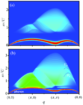
Figure 3: The color maps of $S({\bf q},{\omega})$ along the high-symmetry directions for hopping strength (a) $t/U=0.25$, (b) $t/U=0.4$ at $<n>=0.8$. In (b), the dispersions of $U_{\rm d}$ and $D_{\rm d}$ (blue dotted lines) are the result of $E_{\rm d}$ splitting by doping.

V.1 Molecular excitations at ${\bf q}=[\pi,\pi]$ and its related pairing gap

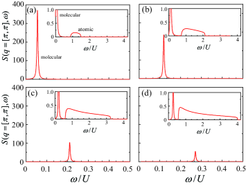
Figure 4: $S({\bf q}=[\pi,\pi],{\omega})$ as a function of $\omega$ for the hopping strength (a) $t/U=0.15$, (b) $t/U=0.25$, (c) $t/U=0.4$, and (d) $t/U=0.5$ at $<n>=0.8$. The inset figures highlight the comparison near the strength of atomic excitations in a large energy region.

Compared with Fig. 2, it can be clearly seen that the dynamical structure factor around $[\pi,\pi]$ moves upward relative to the zero energy at $<n>=0.8$. Then we show that the dynamical structure factor at ${\bf q}=[\pi,\pi]$ can characterize the bosonic molecular excitations (Cooper pairs excitations). To show clearly this physics, the hopping dependence of $S({\bf q},{\omega})$ had been calculated, and the results of $S({\bf q},{\omega})$ as a function of the transfer energy $\omega$ for the hopping strength (a) $t/U=0.15$, (b) $t/U=0.25$, (c) $t/U=0.4$, and (d) $t/U=0.5$ are shown in Fig. 4. The inset figures highlight the comparison near the strength of atomic excitations in a larger energy region. Obviously $S({\bf q},{\omega})$ consists of a sharp peak in the low-energy region and a broad single-particle excitation band in the higher energy region. This sharp peak corresponds to the excitation of the bosonic molecules from a molecular condensate, while the broad single-particle excitation band is the result of atomic (particle-hole) excitations. As the hopping strength $t$ increases (atomic interaction strength decreases), the weight of the molecular peak decreases but the atomic excitation band increases quickly. The variation of the atomic excitation band is shown in the inset figures.

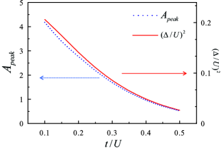
Figure 5: The area of the molecular peak $A_{peak}$ (blue dotted line) and the square of the pairing gap $\Delta^{2}$ (red solid line) as a function of $t$ with $<n>=0.8$.

The weight of the molecular peak can be reflected by calculating the area it covers. We obtain the area of the molecular peak, and plot the area $A_{peak}$ (blue dotted line) as a function of hopping $t$ (Fig. 5), compared with the square of the pairing gap $\Delta^{2}$ (red solid line). Our results show that $A_{peak}$ has the almost same hopping strength dependence as that of $\Delta^{2}$. Both of them are particularly large in a small $t$, and then decrease gradually with $t$ from strong interaction to weak interaction region. Therefore, our results indicate that the $\Delta^{2}$ is responsible for molecular peak at ${\bf q}=[\pi,\pi]$. In other words, experimentally we can measure the pairing gap by detecting the dynamical structure factor at ${\bf q}=[\pi,\pi]$ in the BZ. It is worth noticing that this method to measure pairing gap is universal, and is also suitable for Fermi atoms with spin-orbit coupling (SOC) in optical lattice, where the pairing gap is hard to obtain owing to the complex band structure Zhao2023 .

V.2 The split of $E_{\rm d}$

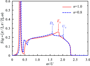
Figure 6: $S({\bf q}=[\pi/2,\pi/2],{\omega})$ as functions of $\omega$ for $n=1.0$ (red solid line), and $n=0.8$ (blue dashed line) at the hopping $t/U=0.4$.

Doping also influence the atomic excitations. Compared with the half-filling case in Fig. 2, the boundary $E_{\rm d}$ has been split owing to doping. To show this clearly, we have calculated the energy dependence of $S({\bf q},{\omega})$ at ${\bf q}=[\pi/2,\pi/2]$. Related results of $S({\bf q},{\omega})$ as a function of ${\omega}$ for $n=1.0$ (red solid line), and $n=0.8$ (blue dashed line) at the hopping strength $t/U=0.4$ are plotted in Fig. 6.

At the low-energy region, a sharp excitation peak appears, and it is the signal of collective phonon mode. Another broad band at larger energy corresponds to the atomic excitations. At half-filling (red solid line) $n=1.0$, a characteristic peak at $\omega/U=1.83$ (marked by the red arrow) appears and corresponds to the $E_{\rm d}$. However, when $n=0.8$, it is seen clearly that $E_{\rm d}$ is split into two branches: $U_{\rm d}$ and $D_{\rm d}$ (marked by two blue dotted line), which is also found in the normal state. So the split of $E_{\rm d}$ is unrelated to the interaction part $H_{\rm int}=-\sum_{{\bf k}}(\Delta^{*}C_{{\bf k}\downarrow}C_{-{\bf k}\uparrow}+H.c.)$ in Eq. 1. Along $[0,0]\rightarrow[\pi,\pi]$, the Fermi momentum $k_{F}=\pi/2$ at $n=1$. As $n$ decreases, the Fermi momentum decreases, which leads to the change of the single-particle excitations.

V.3 Hopping dependence of sound speed

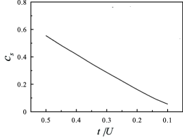
Figure 7: Sound speed $c_{s}$ as a function of $t$ with $<n>=0.8$.

The slope of the Goldstone mode at $\omega\rightarrow 0$ and ${\bf q}\rightarrow 0$ is the sound speed $c_{\rm s}$, $c_{\rm s}=\omega/|{\bf q}|$. The sound speed depends on the interaction strength which can be reflected by the parameter $t/U$. The sound speed $c_{s}$ as a function of $t$ is plotted in Fig. 7. Our theoretical results show that the sound speed decreases with the decreasing hopping strength from weak interaction to strong interaction, which is consistent with the experimental results of Fermi gases ${}^{6}{\rm Li}$ Hoinka17 .

VI Doping dependence of the dynamical structure factor

Then we discussed the dynamical excitations as the doping further increases. Therefore, in Fig. 8, we plot $S({\bf q},{\omega})$ along with the high-symmetry directions of the BZ for (a) $n=0.6$, and (b) $n=0.4$ with $t/U=0.4$.

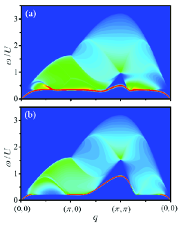
Figure 8: The color maps of $S({\bf q},{\omega})$ for (a) $n=0.6$, and (b) $n=0.4$ with $t/U=0.4$.

Our results show that the molecular excitation peak at ${\bf q}=[\pi,\pi]$ moves to the larger energy, leading to the disappearance of the roton-like dispersion. Moreover, as the doping increases, the gap between $U_{\rm d}$ and $D_{\rm d}$ increases. In particular, the sound speed is doping dependent. To show this issue clearly, we plot the $c_{s}$ as a function of $n$ in Fig. 9.

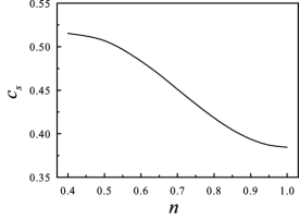
Figure 9: Sound speed $c_{s}$ as a function of $n$ with $t/U=0.4$.

Our results show that the sound speed decreases as $n$ increases. As mentioned above, strong interaction can suppress the sound speed. With the increase of $n$, the interaction between atoms increases, which can explain the doping dependence of the sound speed.

VII Summary

In conclusion, the doping and hopping dependencies of the dynamical structure factor in 2D attractive Fermi-Hubbard model are studied based on RPA theory. First, the area of the molecular excitation peak at ${\bf q}=[\pi,\pi]$ scales with the square of the pairing gap under a certain doping, which potentially indicates a new method to measure the pairing gap qualitatively. Second, a characteristic peak in the atomic excitation band is split into two branches when the system is away from the half-filling, and the gap between them increase for a large doping. Third, the sound speed at given doping is suppressed by a large interaction strength.

VIII Acknowledgements

This work was supported by the funds from the National Natural Science Foundation of China under Grant No.11547034 (H.Z.), Grants No. 11804177 (P.Z.)

IX Appendix

The mean-field response function $\chi^{0}$ of 2D interacting Fermi atoms in square optical lattice is numerically calculated, and all 6 independent matrices elements of $\chi^{0}$ are

$$\chi^{0}_{11} = \frac{1}{4}\sum_{\bf k}\left[1+\frac{\xi_{{\bf k}}\xi_{{\bf k}+{\bf q}}}{E_{{\bf k}}E_{{\bf k}+{\bf q}}}\right]F^{(1)}_{{\bf k},{\bf q}}$$

$$+ \frac{1}{4}\sum_{\bf k}\left[1-\frac{\xi_{{\bf k}}\xi_{{\bf k}+{\bf q}}}{E_{\bf k}E_{{\bf k}+{\bf q}}}\right]F^{(2)}_{{\bf k},{\bf q}},$$

$$\chi^{0}_{12}=-\frac{1}{4}\sum_{\bf k}\frac{\Delta^{2}}{E_{\bf k}E_{{\bf k}+{\bf q}}}\left[F^{(1)}_{{\bf k},{\bf q}}-F^{(2)}_{{\bf k},{\bf q}}\right],$$

$$\chi^{0}_{13}= - \frac{\Delta}{4}\sum_{\bf k}\frac{\xi_{\bf k}+\xi_{{\bf k}+{\bf q}}}{2E_{\bf k}E_{{\bf k}+{\bf q}}}\left[F^{(1)}_{{\bf k},{\bf q}}-F^{(2)}_{{\bf k},{\bf q}}\right]$$

$$+ \frac{\Delta}{4}\sum_{\bf k}\frac{E_{{\bf k}+{\bf q}}-E_{\bf k}}{2E_{\bf k}E_{{\bf k}+{\bf q}}}F^{(3)}_{{\bf k},{\bf q}}$$

$$- \frac{\Delta}{4}\sum_{\bf k}\frac{E_{{\bf k}+{\bf q}}+E_{\bf k}}{2E_{\bf k}E_{{\bf k}+{\bf q}}}F^{(4)}_{{\bf k},{\bf q}},$$

$$\chi^{0}_{14}= - \frac{\Delta}{4}\sum_{\bf k}\frac{\xi_{\bf k}+\xi_{{\bf k}+{\bf q}}}{2E_{\bf k}E_{{\bf k}+{\bf q}}}\left[F^{(1)}_{{\bf k},{\bf q}}-F^{(2)}_{{\bf k},{\bf q}}\right]$$

$$- \frac{\Delta}{4}\sum_{\bf k}\frac{E_{{\bf k}+{\bf q}}-E_{\bf k}}{2E_{\bf k}E_{{\bf k}+{\bf q}}}F^{(3)}_{{\bf k},{\bf q}}$$

$$+ \frac{\Delta}{4}\sum_{\bf k}\frac{E_{{\bf k}+{\bf q}}+E_{\bf k}}{2E_{\bf k}E_{{\bf k}+{\bf q}}}F^{(4)}_{{\bf k},{\bf q}},$$

$$\chi^{0}_{43} = \frac{1}{4}\sum_{\bf k}\left[1-\frac{\xi_{{\bf k}}\xi_{{\bf k}+{\bf q}}}{E_{\bf k}E_{{\bf k}+{\bf q}}}\right]F^{(1)}_{{\bf k},{\bf q}}$$

$$+ \frac{1}{4}\sum_{\bf k}\left[1+\frac{\xi_{{\bf k}}\xi_{{\bf k}+{\bf q}}}{E_{{\bf k}}E_{{\bf k}+{\bf q}}}\right]F^{(2)}_{{\bf k},{\bf q}}$$

$$+ \frac{1}{4}\sum_{\bf k}\left[\frac{\xi_{\bf k}}{E_{\bf k}}-\frac{\xi_{{\bf k}+{\bf q}}}{E_{{\bf k}+{\bf q}}}\right]F^{(3)}_{{\bf k},{\bf q}}$$

$$- \frac{1}{4}\sum_{\bf k}\left[\frac{\xi_{\bf k}}{E_{\bf k}}+\frac{\xi_{{\bf k}+{\bf q}}}{E_{{\bf k}+{\bf q}}}\right]F^{(4)}_{{\bf k},{\bf q}},$$

$$\chi^{0}_{34} = \frac{1}{4}\sum_{\bf k}\left[1-\frac{\xi_{{\bf k}}\xi_{{\bf k}+{\bf q}}}{E_{\bf k}E_{{\bf k}+{\bf q}}}\right]F^{(1)}_{{\bf k},{\bf q}}$$

$$+ \frac{1}{4}\sum_{\bf k}\left[1+\frac{\xi_{{\bf k}}\xi_{{\bf k}+{\bf q}}}{E_{{\bf k}}E_{{\bf k}+{\bf q}}}\right]F^{(2)}_{{\bf k},{\bf q}}$$

$$- \frac{1}{4}\sum_{\bf k}\left[\frac{\xi_{\bf k}}{E_{\bf k}}-\frac{\xi_{{\bf k}+{\bf q}}}{E_{{\bf k}+{\bf q}}}\right]F^{(3)}_{{\bf k},{\bf q}}$$

$$+ \frac{1}{4}\sum_{\bf k}\left[\frac{\xi_{\bf k}}{E_{\bf k}}+\frac{\xi_{{\bf k}+{\bf q}}}{E_{{\bf k}+{\bf q}}}\right]F^{(4)}_{{\bf k},{\bf q}}.$$

The corresponding functions in above equations $F^{(1)}_{{\bf k},{\bf q}}$, $F^{(2)}_{{\bf k},{\bf q}}$, $F^{(3)}_{{\bf k},{\bf q}}$, $F^{(4)}_{{\bf k},{\bf q}}$ are defined as

$$F^{(1)}_{{\bf k},{\bf q}} = A({\bf k},{\bf q},i\omega_{n})-B({\bf k},{\bf q},i\omega_{n}),$$

$$F^{(2)}_{{\bf k},{\bf q}} = C({\bf k},{\bf q},i\omega_{n})-D({\bf k},{\bf q},i\omega_{n}),$$

$$F^{(3)}_{{\bf k},{\bf q}} = A({\bf k},{\bf q},i\omega_{n})+B({\bf k},{\bf q},i\omega_{n}),$$

$$F^{(4)}_{{\bf k},{\bf q}} = C({\bf k},{\bf q},i\omega_{n})+D({\bf k},{\bf q},i\omega_{n}),$$ (15)

where

$$A({\bf k},{\bf q},i\omega_{n}) = \frac{f(E_{\bf k})-f(E_{{\bf k}+{\bf q}})}{i\omega_{n}+(E_{\bf k}-E_{{\bf k}+{\bf q}})}$$

$$B({\bf k},{\bf q},i\omega_{n}) = \frac{f(E_{\bf k})-f(E_{{\bf k}+{\bf q}})}{i\omega_{n}-(E_{\bf k}-E_{{\bf k}+{\bf q}})}$$

$$C({\bf k},{\bf q},i\omega_{n}) = \frac{1-f(E_{\bf k})-f(E_{{\bf k}+{\bf q}})}{i\omega_{n}-(E_{\bf k}+E_{{\bf k}+{\bf q}})}$$

$$D({\bf k},{\bf q},i\omega_{n}) = \frac{1-f(E_{\bf k})-f(E_{{\bf k}+{\bf q}})}{i\omega_{n}+(E_{\bf k}+E_{{\bf k}+{\bf q}})},$$ (16)

$f(E_{\bf k})$ and $f(E_{{\bf k}+{\bf q}})$ are Fermi distributions.

References

- (1) M. Feld, B. Fröhlich, E. Vogt, M. Koschorreck and M. Köhl, Observation of a pairing pseudogap in a two-dimensional Fermi gas, Nature 480, 75 (2011).
- (2) J. T. Stewart, J. P. Gaebler and D. S. Jin, Using photoemission spectroscopy to probe a strongly interacting Fermi gas, Nature 454, 744 (2008).
- (3) B. Fröhlich, M. Feld, E. Vogt, M. Koschorreck, W. Zwerger and M. Köhl, Radio-Frequency Spectroscopy of a Strongly Interacting Two-Dimensional Fermi Gas, Phys. Rev. Lett. 106, 105301 (2011).
- (4) C. Chin, M. Bartenstein, A. Altmeyer, S. Riedl, S. Jochim, J. Hecker Denschlag, and R. Grimm, Observation of the Pairing Gap in a Strongly Interacting Fermi Gas, Science 305, 1128 (2004).
- (5) A. T. Sommer, L. W. Cheuk, M. J. H. Ku, W. S. Bakr, and M. W. Zwierlein, Evolution of Fermion Pairing from Three to Two Dimensions, Phys. Rev. Lett. 108, 045302 (2012).
- (6) H. Zhai, Degenerate quantum gases with spin-orbit coupling: a review, Rep. Prog. Phys. 78, 026001 (2015).
- (7) L. W. Cheuk, A. T. Sommer, Z. Hadzibabic, T. Yefsah, W. S. Bakr, and M. W. Zwierlein, Spin-Injection Spectroscopy of a Spin-Orbit Coupled Fermi Gas, Phys. Rev. Lett. 109, 095302 (2012).
- (8) P. Wang, Z.-Q. Yu, Z. Fu, J. Miao, L. Huang, S. Chai, H. Zhai, and J. Zhang, Spin-Orbit Coupled Degenerate Fermi Gases, Phys. Rev. Lett. 109, 095301 (2012).
- (9) Z.-Y. Wang, X.-C. Cheng, B.-Z. Wang, J.-Y. Zhang, Y.-H. Lu, C.-R. Yi, S. Niu, Y. Deng, X.-J. Liu, S. Chen, and J.-W. Pan, Realization of an ideal Weyl semimetal band in a quantum gas with 3D spin-orbit coupling, Science 372, 271 (2021).
- (10) F. Wu, G.-C. Guo, W. Zhang, and W. Yi, Unconventional Superfluid in a Two-Dimensional Fermi gas with Anisotropic Spin-Orbit Coupling and Zeeman fields, Phys. Rev. Lett. 110, 110401 (2013).
- (11) R. Han, F. Yuan, and H. Zhao, Phase diagram, band structure and density of states in two-dimensional attractive Fermi-Hubbard model with Rashba spin-orbit coupling, New J. Phys. 25, 023001 (2023).
- (12) G. Veeravalli, E. Kuhnle, P. Dyke, and C. J. Vale, Bragg Spectroscopy of a Strongly Interacting Fermi Gas, Phys. Rev. Lett. 101, 250403 (2008).
- (13) S. Hoinka, P. Dyke, M. G. Lingham, J. J. Kinnunen, G. M. Bruun and C. J. Vale, Goldstone mode and pair-breaking excitations in atomic Fermi superfluid, Nat. Phys. 13, 943 (2017).
- (14) H. Biss, L. Sobirey, N. Luick, M. Bohlen, J. J. Kinnunen, G. M. Bruun, T. Lompe, and H. Moritz, Excitation Spectrum and Superfluid Gap of an Ultracold Fermi Gas, Phys. Rev. Lett. 128, 100401 (2022).
- (15) R. Senaratne, D. Cavazos-Cavazos, S. Wang, F. He, Y.-T. Chang, A. Kafle, H. Pu, X.-W. Guan, and R. G. Hulet, Spin-charge separation in a 1D Fermi gas with tunable interactions, Science 376, 1305 (2022).
- (16) X. Li, X. Luo, S. Wang, K. Xie, X. P. Liu, H. Hu, Y.-A. Chen, X.-C. Yao and J. W. Pan, Second sound attenuation near quantum criticality, Science, 375, 528 (2022).
- (17) G. Pagano, M. Mancini, G. Cappellini, P. Lombardi, F. Schöfer, H. Hu, X.-J. Liu, J. Catani, C. Sias, M. Inguscio and L. Fallani, A one-dimensional liquid of fermions with tunable spin, Nat. Phys. 10, 198 (2014).
- (18) R. Combescot, S. Giorgini and S. Stringari, Molecular signatures in the structure factor of an interacting Fermi gas Europhys. Lett. 75, 695 (2006).
- (19) R. Combescot, M. Yu. Kagan, and S. Stringari, Collective mode of homogeneous superfluid Fermi gases in the BEC-BCS crossover, Phys. Rev. A 74, 042717 (2006).
- (20) P. Zou, E. D. Kuhnle, C. J. Vale, and H. Hu, Quantitative comparison between theoretical predictions and experimental results for Bragg spectroscopy of a strongly interacting Fermi superfluid, Phys. Rev. A 82, 061605(R) (2010).
- (21) P. Zou, F. Dalfovo, R. Sharma, X. J. Liu and H. Hu, Dynamic structure factor of a strongly correlated Fermi superfluid within a density functional theory approach, New J. Phys. 18, 113044 (2016).
- (22) P. Zou, H. Hu, and X.-J. Liu, Low-momentum dynamic structure factor of a strongly interacting Fermi gas at finite temperature: The Goldstone phonon and its Landau damping, Phys. Rev. A 98, 011602(R) (2018).
- (23) H. Hu, P. Zou, and X.-J. Liu, Low-momentum dynamic structure factor of a strongly interacting Fermi gas at finite temperature: A two-fluid hydrodynamic description, Phys. Rev. A 97, 023615 (2018).
- (24) P. Zou, H. Zhao, L. He, X.-J. Liu, and H. Hu, Dynamic structure factors of a strongly interacting Fermi superfluid near an orbital Feshbach resonance across the phase transition from BCS to Sarma superfluid, Phys. Rev. A 103, 053310 (2021).
- (25) E. D. Kuhnle, H. Hu, X.-J. Liu, P. Dyke, M. Mark, P. D. Drummond, P. Hannaford, and C. J. Vale, Universal Behavior of Pair Correlations in a Strongly Interacting Fermi Gas, Phys. Rev. Lett. 105, 070402 (2010).
- (26) S. Watabe, and T. Nikuni, Dynamic structure factor of the normal Fermi gas from the collisionless to the hydrodynamic regime, Phys. Rev. A 82, 033622 (2010).
- (27) E. Vitali, H. Shi, M. Qin, and S. Zhang, Visualizing the BEC-BCS crossover in a two-dimensional Fermi gas:Pairing gaps and dynamical response functions from ab initio computations, Phys. Rev. A 96, 061601(R) (2017).
- (28) H. Zhao, X. Gao, W. Liang, P. Zou and F. Yuan, Dynamical structure factors of a two-dimensional Fermi superfluid within random phase approximation, New J. Phys. 22, 093012 (2020).
- (29) Z. Gao, L. He, H. Zhao, S.-G. Peng, and P. Zou, Dynamic structure factor of one-dimensional Fermi superfluid with spin-orbit coupling, Phys. Rev. A 107, 013304 (2023).
- (30) I. Bloch, J. Dalibard and W. Zwerger, Many-body physics with ultracold gases, Rev. Mod. Phys. 80, 885 (2008).
- (31) Z. Wu, L. Zhang, W. Sun, X.-T. Xu, B.-Z. Wang, S.-C. Ji, Y. Deng, S. Chen, X.-J. Liu, and J.-W. Pan, Realization of two-dimensional spin-orbit coupling for Bose-Einstein condensates, Science 354, 83 (2016).
- (32) M. Greiner, O. Mandel, T. Esslinger, T. W. Hänsch, and I. Bloch, Quantum phase transition from a superfluid to a Mott insulator in a gas of ultracold atoms, Nature 415, 39 (2002).
- (33) I. B. Spielman, W. D. Phillips, and J. V. Porto, Condensate Fraction in a 2D Bose Gas Measured across the Mott-Insulator Transition, Phys. Rev. Lett. 100, 120402 (2008).
- (34) C. K. Thomas, T. H. Barter, T.-H. Leung, M. Okano, G.-B. Jo, J. Guzman, I. Kimchi, A. Vishwanath, and D. M. Stamper-Kurn, Mean-Field Scaling of the Superfluid to Mott Insulator Transition in a 2D Optical Superlattice, Phys. Rev. Lett. 119, 100402 (2017).
- (35) R. Jördens, N. Strohmaier, K. Günter, H. Moritz, and T. Esslinger, A Mott insulator of fermionic atoms in an optical lattice, Nature 455, 204 (2008).
- (36) U. Schneider, L. Hackermüller, S. Will, Th. Best, I. Bloch, T. A. Costi, R. W. Helmes, D. Rasch, and A. Rosch, Metallic and insulating phases of repulsively interacting fermions in a 3D optical lattice, Science 322, 1520 (2008).
- (37) D. Greif, T. Uehlinger, G. Jotzu, L. Tarruell, and T. Esslinger, Short-range quantum magnetism of ultracold fermions in an optical lattice, Science 340, 1307 (2013).
- (38) R. A. Hart, P. M. Duarte, T.-L. Yang, X. Liu, T. Paiva, E. Khatami, R. T. Scalettar, N. Trivedi, D. A. Huse, and R. G. Hulet, Observation of antiferromagnetic correlations in the Hubbard model with ultracold atoms, Nature 519, 211 (2015).
- (39) M. F. Parsons, A. Mazurenko, C. S. Chiu, G. Ji, D. Greif and M. Greiner, Site-resolved measurement of the spin-correlation function in the Fermi-Hubbard model, Science 353, 1253 (2016).
- (40) L. W. Cheuk, M. A. Nichols, K. R. Lawrence, M. Okan, H. Zhang, E. Khatami, N. Trivedi, T. Paiva, M. Rigol, and M. W. Zwierlein, Observation of spatial charge and spin correlations in the 2D Fermi-Hubbard model, Science 353, 1260 (2016).
- (41) J. Koepsell, D. Bourgund, P. Sompet, S. Hirthe, A. Bohrdt, Y. Wang, F. Grusdt, E. Demler, G. Salomon, C. Gross, and I. Bloch, Microscopic evolution of doped Mott insulators from polaronic metal to Fermi liquid, Science 374, 82 (2021).
- (42) M. Boll, T. A. Hilker, G. Salomon, A. Omran, J. Nespolo, L. Pollet, I. Bloch, and C. Gross, Spin-and density-resolved microscopy of antiferromagnetic correlations in Fermi-Hubbard chains, Science 353, 1257 (2016).
- (43) P. T. Brown, D. Mitra, E. Guardado-Sanchez, P. Schauß, S. S. Kondov, E. Khatami, T. Paiva, N. Trivedi, D. A. Huse, and W. S. Bakr, Spin-imbalance in a 2D Fermi-Hubbard system, Science 357, 1385 (2017).
- (44) R. T. Scalettar, E. Y. Loh, J. E. Gubernatis, A. Moreo, S. R. White, D. J. Scalapino, R. L. Sugar, and E. Dagotto. Phase diagram of the two-dimensional negative- Hubbard model, Phys. Rev. Lett. 62, 1407 (1989).
- (45) B. Kyung, S. Allen, and A.-M. S. Tremblay, Pairing fluctuations and pseudogaps in the attractive Hubbard model. Phys. Rev. B 64, 075116 (2001).
- (46) C. Honerkamp, and W. Hofstetter, Ultracold Fermions and the SU(N) Hubbard Model, Phys. Rev. Lett. 92, 170403 (2004).
- (47) R. Mondaini, P. Nikolić, and M. Rigol, Mott-insulator-to-superconductor transition in a two-dimensional superlattice, Phys. Rev. A 92, 013601 (2015).
- (48) E. Cocchi, L. A. Miller, J. H. Drewes, M. Koschorreck, D. Pertot, F. Brennecke, and M. Köhl, Equation of state of the two-dimensional Hubbard model, Phys. Rev. Lett. 116, 175301 (2016).
- (49) N. Strohmaier, Y. Takasu, K. Günter, R. Jördens, M. Köhl, H. Moritz, and T. Esslinger, Interaction-controlled transport of an ultracold Fermi gas, Phys. Rev. Lett. 99, 220601 (2007).
- (50) A. F. Ho, M. A. Cazalilla, and T. Giamarchi, Quantum simulation of the Hubbard model: the attractive route, Phys. Rev. A 79, 033620 (2009).
- (51) A. Moreo, D. J. Scalapino, Cold attractive spin polarized Fermi lattice gases and the doped positive Hubbard model, Phys. Rev. Lett. 98, 216402 (2007).
- (52) J. Gukelberger, S. Lienert, E. Kozik, L. Pollet, and M. Troyer, Fulde-Ferrell-Larkin-Ovchinnikov pairing as leading instability on the square lattice, Phys. Rev. B 94, 075157 (2016).
- (53) T. Paiva, R. R. dos Santos, R. T. Scalettar, and P. J. H. Denteneer, Critical temperature for the two-dimensional attractive Hubbard model, Phys. Rev. B 69, 184501 (2004).
- (54) V. B. Shenoy, Phase diagram of the attractive Hubbard model with inhomogeneous interactions, Phys. Rev. B 78, 134503 (2008).
- (55) D. Mitra, P. T. Brown, E. Guardado-Sanchez, S. S. Kondov, T. Devakul, D. A. Huse, P. Schauß, and W. S. Bakr, Quantum gas microscopy of an attractive Fermi-Hubbard system, Nat. Phys. 14, 173 (2018).
- (56) P. T. Brown, E. Guardado-Sanchez, B. M. Spar, E. W. Huang, T. P. Devereaux, and W. S. Bakr, Angle-resolved photoemission spectroscopy of a Fermi-Hubbard system, Nat. Phys. 16, 26 (2020).
- (57) L. Hackermüller, U. Schneider, M. Moreno-Cardoner, T. Kitagawa, T. Best, S. Will, E. Demler, E. Altman, I. Bloch, and B. Paredes, Anomalous Expansion of Attractively Interacting Fermionic Atoms in an Optical Lattice, Science 327, 1621 (2010).
- (58) M. Gall, C. F. Chan, N. Wurz, and M. Köhl, Simulating a Mott Insulator Using Attractive Interaction, Phys. Rev. Lett. 124, 010403 (2020).
- (59) U. Schneider, L. Hackermüller, J. P. Ronzheimer, S. Will, S. Braun, T. Best, I. Bloch, E. Demler, S. Mandt, D. Rasch, and A. Rosch, Fermionic transport and out-of-equilibrium dynamics in a homogeneous Hubbard model with ultracold atoms, Nat. Phys. 8, 213 (2012).
- (60) E. Vitali, P. Kelly, A. Lopez, G. Bertaina, and D. E. Galli, Dynamical structure factor of a fermionic supersolid on an optical lattice, Phys. Rev. A 102, 053324 (2020).
- (61) H. Zhao, R. Han, F. Yuan, and P. Zou, unsummited.
- (62) X.-J. Liu, H. Hu, A. Minguzzi, and M. P. Tosi, Collective oscillations of a confined Bose gas at finite temperature in the random-phase approximation, Phys. Rev. A 69, 043605 (2004).
- (63) R. Han, F. Yuan, and H. Zhao, Single-particle excitations and metal-insulator transition of ultracold Fermi atoms in one-dimensional optical lattice with spin-orbit coupling, Europhys. Lett. 139, 25001 (2022).
- (64) A. Nocera, N. D. Patel, J. Fernandez-Baca, E. Dagotto, and G. Alvarez, Magnetic excitation spectra of strongly correlated quasi-one-dimensional systems: Heisenberg versus Hubbard-like behavior, Phys. Rev. B 94, 205145 (2016).