Noether Symmetries and Anisotropic Universe in Energy-Momentum Squared Gravity

Abstract

This paper explores exact cosmological solutions of anisotropic universe model through Noether symmetry technique in energy-momentum squared gravity. This theory resolves the primordial singularity and provides viable cosmological consequences in the early universe. We consider specific models of this theory and evaluate Noether equations, symmetry generators and corresponding conserved parameters. We then find exact solutions through conserved parameters and analyze their graphical behavior for different cosmological parameters. It is found that the behavior of these parameters is consistent with recent observations indicating that this theory supports current cosmic accelerated expansion. We conclude that conserved parameters are very helpful to obtain exact cosmological solutions.

Keywords: Energy-momentum squared gravity; Noether symmetries; Conserved parameters; Exact anisotropic solutions.
PACS: 04.20.Jb; 98.80.-k; 04.50.Kd; 98.80.Jk.

1 Introduction

The current cosmic acceleration has been the most dazzling and interesting outcome for cosmologists over the last two decades. Several cosmological observations such as supernovae type Ia, cosmic microwave background (CMB), Planck data, etc., justify that the universe is in the accelerated expansion phase [1]. Scientists believe that this expansion is the outcome of an enigmatic force known as dark energy (DE) which has large negative pressure. This ambiguous force has inspired many scientists to uncover its hidden aspects. Einstein introduced cosmological constant $(\Lambda)$ in his field equations to explain the mysterious aspects of DE which is known as the cosmological constant cold dark matter ($\Lambda$CDM) model. But, this approach has two main issues such as fine-tuning and coincidence problems. The first issue arises because of the large difference between observed and predicted values of energy density whereas the second problem describes that if the energy densities of DE and dark matter (DM) are identical then why current cosmic acceleration is observed? [2].

Several modifications of general relativity (GR) have proposed different approaches to solve these problems dubbed as modified theories. These proposals are assumed as the most elegant and significant approaches to reveal the dark universe. These theories are developed by modifying the geometric and matter parts of the Einstein-Hilbert (EH) action. The strong relation between gravity and relativistic objects at cosmological scales indicates that alternative gravitational theories should be established from the curvature part of the EH action. The simplest modification of GR is $f(\mathcal{R})$ gravity which is constructed by substituting the generic function of Ricci scalar $(\mathcal{R})$ in the curvature part of the EH action. To understand the viability of this theory, detailed literature has been made available in [3].

The $f(\mathcal{R})$ theory has further been modified by including some interactions between geometric and matter parts. These interactions describe the rotation curves of galaxies and different cosmic evolutionary eras. An additional force appears in this framework due to the non-conserved stress-energy tensor and results in the non-geodesic motion of the particles. These interaction proposals are extremely helpful to comprehend mysterious aspects of the cosmos. The coupling of matter-Lagrangian $(\mathrm{L}_{\mathrm{M}})$ and curvature has been introduced in [4] named $f(\mathcal{R},\mathrm{L}_{\mathrm{M}})$ theory. The non-minimal interection between geometric and matter sectors was formulated in [5] named $f(\mathcal{R},\mathrm{T},\mathcal{R}_{\mu\nu}\mathrm{T}^{\mu\nu})$ gravity, where the stress-energy tensor is denoted by $\mathrm{T}$.

The presence of singularities is considered the most critical issue in GR as these are predicted at large regimes, where GR is invalid due to quantum impacts. In this perspective, a new generalization to GR has been established by adding a non-linear term $(\mathbf{T}^{2}=\mathrm{T}^{\mu\nu}\mathrm{T}_{\mu\nu})$ in the generic action named $f(\mathcal{R},\mathbf{T}^{2})$ theory which is also known as energy-momentum squared gravity (EMSG) [6]. This theory provides a specific relation between curvature and matter parts and contains an extra force $(\mathrm{T}^{\mu\nu}\mathrm{T}_{\mu\nu})$ together with $f(\mathcal{R})$ which gives a better description to expose the mysterious universe. The field equations include squared and product entities of fluid parameters that are helpful to describe various cosmological results. This approach has a small-scale parameter corresponding to finite maximum energy density. As a result, it has a bounce in the early times and resolves primordial singularity. It is worth mentioning here that this theory describes the complete cosmic history including the inflationary era as well as cosmic evolution similar to that in the $\Lambda$CDM model.

The analytic solutions of isotropic spacetime with a specific EMSG model have been discussed in [7]. The physically viable compact objects and hydrostatic equilibrium equations have been studied in [8]. Different coupling models of EMSG have been analyzed and found that the proposed models can explain the current cosmic acceleration [9]. Barbar et al [10] examined viability of the bouncing universe in the same theory and explored that our universe was non-singular in the early times. The geometry of self-gravitating objects with quark matter and thermodynamic characteristics of a black hole have been analyzed in [11]. Recently, we have examined the dynamics of spherical as well as cylindrical collapse with various matter distributions in this framework and found that modified terms of EMSG reduces the collapse rate [12]. The preceding literature demonstrates that this theory requires more consideration in different contexts.

Many cosmic observations such as Wilkinson Microwave Anisotropy Probe, Planck satellites and CMB indicate that the current cosmos is isotropic and homogeneous at large scales. This cosmic stage is determined by the Friedmann-Robertson-Walker (FRW) spacetime, which ignores the anisotropy as well as all cosmic structures. However, the universe was discovered to be spatially homogeneous and anisotropic at the early times. The anisotropy is still analyzed in the present cosmos as a CMB temperature. Bianchi type (BT) universe models are considered the most significant and captivating models which can explain the impact of anisotropy in the early times. These anisotropic models demonstrate that the initial anisotropy affects the fate of rapid expansion which will continue for large values of anisotropy. If the initial anisotropy is minor then the rapid cosmic expansion will stop leading to a highly isotropic cosmos [13].

Many researchers have studied these models from various perspectives. Akarsu and Kilinc [14] analyzed the BT-I model with anisotropic fluid and found that the constant effective energy density and equation of state (EoS) variable are responsible for cosmic expansion. Yadav and Saha [15] examined the BT-I cosmological model with dominance of DE and found that DE leads to the current cosmic accelerated expansion. Adhav [16] investigated exact cosmological solutions of anisotropic universe in $f(\mathcal{R},\mathrm{T})$ gravity. Shamir [17] discussed exact solutions of the BT-I universe and analyzed their behavior through different physical parameters in the same gravity. Sharif and Jabbar [18] studied the stability criteria of the BT-I spacetime in $f(\mathcal{T})$ gravity, where $\mathcal{T}$ is the torsion scalar.

Symmetry plays a crucial role in the study of cosmology and gravitational physics. Accordingly, Noether symmetry technique is considered the most efficient approach that describes a correlation between symmetry generators and conserved parameters of a physical system [19]. This method is widely used to investigate exact solutions in various aspects which are then discussed in terms of cosmic features. Moreover, this technique gives a useful method to establish conserved quantities. The conservation laws are most important in analyzing various physical phenomena. These laws are the specific cases of Noether theorem which states that every action with a differentiable symmetry yields conservation law. This theorem is significant as it gives a link among conserved parameters and symmetries of a dynamical system [20]. A lot of interesting work has been examined in this framework [21].

Noether symmetries have several useful applications in alternative gravitational theories. Capozziello et al [22] found exact cosmological solutions of spherical spacetimes through Noether symmetry approach in $f(\mathcal{R})$ theory. Shamir et al [23] examined the stability of $f(\mathcal{R})$ models for static sphere and FRW universe model through this approach. Kucukakca [24] formulated exact isotopic solutions through Noether symmetry in the scalar-tensor theory. Sharif and Waheed [25] investigated BT-I and FRW spacetimes through Noether symmetries in the same theory. Sharif and Shafique [26] investigated the BT-I spacetime through Noether symmetries in scalar-field gravity. Momeni et al. [27] analyzed exact cosmological solutions through Noether symmetries in $f(\mathcal{R},\mathrm{T})$ theory.

Sharif and Fatima [28] derived exact cosmological solutions of the FRW universe by Noether symmetries in $f(\mathrm{G})$ theory, where $G$ is the Gauss-Bonnet term and examined the cosmic acceleration in terms of the scale parameter. Shamir and Ahmad [29] examined various cosmological solutions with different fluid configurations in $f(\mathrm{G},\mathrm{T})$ gravity. Bahamonde et al [30] used this technique to examine new exact spherical solutions in $f(\mathcal{R},\phi,\chi)$ gravity, where $\phi$ is a scalar field and $\chi$ defines the kinetic term of $\phi$. Bahamonde et al [31] used Noether symmetry technique to obtain wormhole solutions in $f(\mathcal{T})$ theory. Recently, we have obtained exact cosmological solutions in $f(\mathcal{R},\mathbf{T}^{2})$ gravity and analyzed their behavior through various physical quantities [32]. We have also investigated wormhole solutions and geometry of compact stellar objects in this background [33].

This paper examines Noether symmetries for BT-I universe in the context of EMSG. We determine symmetry generators with corresponding conserved parameters to find exact cosmological solutions for different EMSG models and examine their graphical behavior through different physical parameters. The plan of the article is as follows. Section 2 investigates basic formalism of EMSG. Section 3 provides a detailed analysis of Noether symmetries. In section 4, we derive exact BT-I solutions using Noether symmetries and discuss them through graphs. We summarize our results in the last section.

2 Energy-Momentum Squared Gravity

This section formulates the equations of motion with perfect matter configuration in the framework of EMSG. The EH action of this modified gravity is defined as [6]

$$S=\int\sqrt{-g}\left(\frac{f\left(\mathcal{R},\mathbf{T}^{2}\right)}{2\kappa^{2}}+\mathrm{L}_{\mathrm{M}}\right)d^{4}x,$$ (1)

where $\kappa^{2}$ is coupling constant. Here, the possibility of exact solutions is increased than GR due to the presence of extra degrees of freedom. It is assumed that some significant results will be achieved to examine the current cosmic acceleration because of the matter source. The following field equations are formulated by varying the action corresponding to the metric tensor

$$\mathcal{R}_{\mu\nu}f_{\mathcal{R}}+g_{\mu\nu}\Box f_{\mathcal{R}}-\nabla_{\mu}\nabla_{\nu}f_{\mathcal{R}}-\frac{1}{2}g_{\mu\nu}f=\mathrm{T}_{\mu\nu}-\Theta_{\mu\nu}f_{\mathbf{T}^{2}},$$ (2)

where $f\equiv f(\mathcal{R},\mathbf{T}^{2})$, $f_{\mathbf{T}^{2}}=\frac{\partial f}{\partial\mathbf{T}^{2}}$, $f_{\mathcal{R}}=\frac{\partial f}{\partial\mathcal{R}}$, $\Box=\nabla_{\mu}\nabla^{\mu}$ and

$$\Theta_{\mu\nu}=-2\mathrm{L}_{\mathrm{M}}\left(\mathrm{T}_{\mu\nu}-\frac{1}{2}g_{\mu\nu}\mathrm{T}\right)-4\frac{\partial^{2}\mathrm{L}_{\mathrm{M}}}{\partial g^{\mu\nu}\partial g^{\alpha\beta}}\mathrm{T}^{\alpha\beta}-\mathrm{T}\mathrm{T}_{\mu\nu}+2\mathrm{T}_{\mu}^{\alpha}\mathrm{T}_{\nu\alpha}.$$ (3)

The energy-momentum tensor describes the matter configuration in gravitational physics and gives dynamical variables with specific physical characteristics. We consider isotropic fluid configuration as

$$\mathrm{T}_{\mu\nu}=(\rho+\mathrm{p})\mathrm{U}_{\mu}\mathrm{U}_{\nu}+\mathrm{p}g_{\mu\nu},$$ (4)

Rearranging Eq.(2), we have

$$\mathcal{G}_{\mu\nu}=\frac{1}{f_{\mathcal{R}}}\left(\mathrm{T}_{\mu\nu}^{(\mathrm{D})}+\mathrm{T}_{\mu\nu}\right)=\mathrm{T}_{\mu\nu}^{eff},$$ (5)

where Einstein tensor is denoted by $\mathcal{G}_{\mu\nu}$ and $\mathrm{T}_{\mu\nu}^{(D)}$ represents the additional effects of EMSG that contain higher-order curvature terms due to the modification in geometric part expressed as

$$\mathrm{T}_{\mu\nu}^{(\mathrm{D})}=\frac{1}{2}g_{\mu\nu}\left(f-\mathcal{R}f_{\mathcal{R}}\right)-g_{\mu\nu}\Box f_{\mathcal{R}}+\nabla_{\mu}\nabla_{\nu}f_{\mathcal{R}}-\Theta_{\mu\nu}f_{\mathbf{T}^{2}}.$$ (6)

Equation (5) determines that the dark source terms provide matter contents of the universe. These additional terms contain all the fluid elements that could be useful to reveal the dark characteristics of the universe.

In order to analyze the anisotropic universe, we consider BT-I universe model as

$$ds^{2}=-d\mathrm{t}^{2}+\mathrm{a}^{2}(\mathrm{t})d\mathrm{x}^{2}+\mathrm{b}^{2}(\mathrm{t})(d\mathrm{y}^{2}+d\mathrm{z}^{2}).$$ (7)

The resulting equations of motion become

$$\rho^{eff} = \frac{1}{f_{\mathcal{R}}}\left[\rho-\frac{1}{2}f+(3\mathrm{p}^{2}+\mathrm{\rho}^{2}+4\mathrm{p}\mathrm{\rho})f_{\mathbf{T}^{2}}-(\dot{\mathrm{a}}\mathrm{a}^{-1}+2\dot{\mathrm{b}}\mathrm{b}^{-1})\right.$$ (8)

$$\times \left.(\dot{\mathcal{R}}f_{\mathcal{R}\mathcal{R}}+\dot{\mathbf{T}}^{2}f_{\mathcal{R}\mathbf{T}^{2}})+\frac{1}{2}\mathcal{R}f_{\mathcal{R}}\right],$$

$$\mathrm{p}^{eff} = \frac{1}{f_{\mathcal{R}}}\left[\mathrm{p}+\frac{1}{2}(f-\mathcal{R}f_{\mathcal{R}})+2\dot{\mathrm{b}}\mathrm{b}^{-1}(\dot{\mathcal{R}}f_{\mathcal{R}\mathcal{R}}+\dot{\mathbf{T}}^{2}f_{\mathcal{R}\mathbf{T}^{2}})+\ddot{\mathcal{R}}f_{\mathcal{R}\mathcal{R}}\right.$$ (9)

$$+ \left.\ddot{\mathbf{T}}^{2}f_{\mathcal{R}\mathbf{T}^{2}}+\dot{\mathcal{R}}^{2}f_{\mathcal{R}\mathcal{R}\mathcal{R}}+\dot{\mathbf{T}}^{2}f_{\mathcal{R}\mathbf{T}^{2}\mathbf{T}^{2}}+2\dot{\mathcal{R}}\dot{\mathbf{T}}f_{\mathcal{R}\mathcal{R}\mathbf{T}^{2}}\right],$$

$$\mathrm{p}^{eff} = \frac{1}{f_{\mathcal{R}}}\left[\mathrm{p}+\frac{1}{2}(f-\mathcal{R}f_{\mathcal{R}})+(\dot{\mathrm{a}}\mathrm{a}^{-1}+\dot{\mathrm{b}}\mathrm{b}^{-1})(\dot{\mathcal{R}}f_{\mathcal{R}\mathcal{R}}+\dot{\mathbf{T}}^{2}f_{\mathcal{R}\mathbf{T}^{2}})+\ddot{\mathcal{R}}f_{\mathcal{R}\mathcal{R}}\right.$$ (10)

$$+ \left.\ddot{\mathbf{T}}^{2}f_{\mathcal{R}\mathbf{T}^{2}}+\dot{\mathcal{R}}^{2}f_{\mathcal{R}\mathcal{R}\mathcal{R}}+\dot{\mathbf{T}}^{2}f_{\mathcal{R}\mathbf{T}^{2}\mathbf{T}^{2}}+2\dot{\mathcal{R}}\dot{\mathbf{T}}f_{\mathcal{R}\mathcal{R}\mathbf{T}^{2}}\right],$$

where the dot is derivative corresponding to the temporal coordinate. The analysis of analytic solutions in alternative gravitational theories has attained much attention in recent years to study cosmic evolution and acceleration. The direct solution of the above equations is very difficult due to their highly non-linear nature. There are two possible ways to solve these equations. One is to solve them by applying suitable exact or numeric method whereas 2nd is to obtain exact solutions by Noether symmetry technique. This theory is non-conserved but conserved quantities can be examined by Noether symmetries. Thus the latter approach appears to be more interesting and we adopt it in this article.

3 Noether Symmetries

Noether symmetries offer an interesting method to establish new cosmological models and associated structures in modified theories. This section develops point-like Lagrangian and determines the corresponding Noether equations for the BT-I universe in the context of EMSG. This technique yields a unique vector field corresponding to tangent space. Thus, the vector field acts as a symmetry generator and gives conserved parameters that are useful to investigate exact cosmological solutions.

The action (1) in canonical form becomes

$$\mathcal{S}=\int\mathrm{L}(\mathrm{a},\dot{\mathrm{a}},\mathrm{b},\dot{\mathrm{b}},\mathcal{R},\dot{\mathcal{R}},\mathbf{T}^{2},\dot{\mathbf{T}^{2}})dt.$$ (11)

To obtain point-like Lagrangian, we use the Lagrange multiplier technique as

$$\mathcal{S}=\int(f+\mathrm{p}-(\mathcal{R}-\bar{\mathcal{R}})\lambda_{1}-(\mathbf{T}^{2}-\mathbf{\bar{T}}^{2})\lambda_{2})\sqrt{-g}d\mathrm{t},$$ (12)

where

$$\bar{\mathcal{R}}=2\left(\frac{\ddot{\mathrm{a}}}{\mathrm{a}}+\frac{2\ddot{\mathrm{b}}}{\mathrm{b}}+\frac{2\dot{\mathrm{a}}\dot{\mathrm{b}}}{\mathrm{a}\mathrm{b}}+\frac{\dot{\mathrm{b}}^{2}}{\mathrm{b}^{2}}\right),\quad\bar{\mathbf{T}}^{2}=3\mathrm{p}^{2}+\rho^{2},\quad\lambda_{1}=f_{\mathcal{R}},\quad\lambda_{2}=f_{\mathbf{T}^{2}}.$$

We observe that the action (1) for BT-I spacetime is recovered when $\mathcal{R}-\bar{\mathcal{R}}=0$ and $\mathbf{T}^{2}-\bar{\mathbf{T}^{2}}=0$. Substituting the above values in Eq.(12), we have

$$\mathrm{L} = \mathrm{a}\mathrm{b}^{2}(f+\mathrm{p})-2(\mathrm{a}\dot{\mathrm{b}}^{2}+2\dot{\mathrm{a}}\dot{\mathrm{b}}\mathrm{b})f_{\mathcal{R}}+\mathrm{a}\mathrm{b}^{2}\left(3\mathrm{p}^{2}+\rho^{2}\right)f_{\mathbf{T}^{2}}-2$$ (13)

$$\times (\dot{\mathrm{a}}\mathrm{b}^{2}+2\mathrm{a}\mathrm{b}\dot{\mathrm{b}})(\dot{\mathcal{R}}f_{\mathcal{R}\mathcal{R}}+\dot{\mathbf{T}}^{2}f_{\mathcal{R}\mathbf{T}^{2}})-\mathrm{a}\mathrm{b}^{2}\left(\mathcal{R}f_{\mathcal{R}}+\mathbf{T}^{2}f_{\mathbf{T}^{2}}\right).$$

It is noteworthy to mention here that when $\mathrm{a}(\mathrm{t})=\mathrm{b}(\mathrm{t})$, the Lagrangian of FRW universe is recovered [32]. The above Lagrangian is difficult due to its highly non-linear nature. Therefore, we need some additional constraints to solve it. Here we use a physical condition that the ratio of shear scalar $(\sigma)$ to expansion scalar $(\Theta)$ is constant, which gives $\mathrm{a}=\mathrm{b}^{n}$, where $n$ is a real constant and we consider $n\neq 0,1$ for non-trivial solution. This condition suggests that the Hubble cosmic expansion can achieve isotropy when $\frac{\sigma}{\Theta}$ is constant [34]. Several researchers have also used this relation to obtain the cosmological solutions [35]. Thus, the Lagrangian (13) becomes

$$\mathrm{L} = \mathrm{b}^{n+2}(f+\mathrm{p})-\mathrm{b}^{n+2}\left(\mathcal{R}f_{\mathcal{R}}+\mathbf{T}^{2}f_{\mathbf{T}^{2}}\right)+\mathrm{b}^{n+2}\left(3\mathrm{p}^{2}+\rho^{2}\right)f_{\mathbf{T}^{2}}$$ (14)

$$- 2(\mathrm{b}^{n}\dot{\mathrm{b}}^{2}+2n\mathrm{b}^{n}\dot{\mathrm{b}}^{2})f_{\mathcal{R}}-2\mathrm{b}^{n+1}\dot{\mathrm{b}}(n+2)(\dot{\mathcal{R}}f_{\mathcal{R}\mathcal{R}}+\dot{\mathbf{T}}^{2}f_{\mathcal{R}\mathbf{T}^{2}}).$$

The corresponding Hamiltonian, $\mathcal{H}=\dot{q}^{i}(\partial\mathrm{L}/\partial\dot{q}^{i})-\mathrm{L}$ is given by

$$\mathcal{H} = \mathrm{b}^{n+2}\left(\mathcal{R}f_{\mathcal{R}}+\mathbf{T}^{2}f_{\mathbf{T}^{2}}\right)-\mathrm{b}^{n+2}\left(3\mathrm{p}^{2}+\rho^{2}\right)f_{\mathbf{T}^{2}}-\mathrm{b}^{n+2}(f+\mathrm{p})$$ (15)

$$- 2(\mathrm{b}^{n}\dot{\mathrm{b}}^{2}+2n\mathrm{b}^{n}\dot{\mathrm{b}}^{2})f_{\mathcal{R}}-2\mathrm{b}^{n+1}\dot{\mathrm{b}}(n+2)\dot{f_{\mathcal{R}}}.$$

The symmetry generators of the Lagrangian (14) are given by

$$\mathrm{K}=\xi(\mathrm{t},\mathrm{b},\mathcal{R},\mathbf{T}^{2})\frac{\partial}{\partial t}+\eta^{i}(\mathrm{t},\mathrm{b},\mathcal{R},\mathbf{T}^{2})\frac{\partial}{\partial q^{i}},\quad i=1,2,3,$$ (16)

where undetermined coefficients of $\mathrm{K}$ are represented by $\xi$ and $\eta^{i}=(\alpha,\beta,\gamma)$, respectively. For the existence of Noether symmetries, the Lagrangian must fulfill the invariance condition defined as

$$\mathrm{K}^{[1]}\mathrm{L}+(\mathfrak{D}\xi)\mathrm{L}=\mathfrak{D}\psi,$$ (17)

where the total rate of change, first-order prolongation, and boundary term are denoted by $\mathfrak{D}$, $\mathrm{K}^{[1]}$ and $\psi$, respectively. Further, it is expressed as

$$\mathrm{K}^{[1]}=\mathrm{K}+\dot{\eta}^{i}\frac{\partial}{\partial\dot{q}^{i}},~{}~{}~{}\mathfrak{D}=\frac{\partial}{\partial t}+\dot{q}^{i}\frac{\partial}{\partial q^{i}},$$ (18)

here $\dot{\eta}^{i}$=$\mathfrak{D}\eta^{i}-\dot{q}^{i}\mathfrak{D}\xi$. The corresponding conserved quantities are defined as

$$\mathcal{I}=\eta^{i}\frac{\partial\mathrm{L}}{\partial\dot{q}^{i}}-\xi\mathcal{H}-\psi.$$ (19)

This is also dubbed as the first integral of motion and considered the most crucial part of Noether symmetries which play a significant role to determine viable cosmological solutions.

We formulate the following system of partial differential equations (PDEs) by evaluating and comparing the coefficients of Eq.(17)

$$\xi_{\mathrm{b}}=0,\quad\xi_{\mathcal{R}}=0,\quad\xi_{\mathbf{T}^{2}}=0,$$ (20)

$$(2+n)\mathrm{b}^{n+1}\alpha_{\mathcal{R}}f_{\mathcal{R}\mathcal{R}}=0,\quad 4\mathrm{b}^{n+1}\alpha_{\mathrm{t}}f_{\mathcal{R}\mathcal{R}}+2n\mathrm{b}^{n+1}\alpha_{\mathrm{t}}f_{\mathcal{R}\mathcal{R}}-\psi_{\mathcal{R}}=0,$$ (21)

$$(2+n)\mathrm{b}^{n+1}\alpha_{\mathbf{T}^{2}}f_{\mathcal{R}\mathbf{T}^{2}}=0,\quad 4\mathrm{b}^{n+1}\alpha_{\mathrm{t}}f_{\mathcal{R}\mathbf{T}^{2}}+2n\mathrm{b}^{n+1}\alpha_{\mathrm{t}}f_{\mathcal{R}\mathbf{T}^{2}}-\psi_{\mathbf{T}^{2}}=0,$$ (22)

$$4\mathrm{b}^{n+1}\alpha_{\mathbf{T}^{2}}f_{\mathcal{R}\mathcal{R}}+2n\mathrm{b}^{n+1}\alpha_{\mathbf{T}^{2}}f_{\mathcal{R}\mathcal{R}}+4\mathrm{b}^{n+1}\alpha_{\mathcal{R}}f_{\mathcal{R}\mathbf{T}^{2}}+2n\mathrm{b}^{n+1}\alpha_{\mathcal{R}}f_{\mathcal{R}\mathbf{T}^{2}}=0,$$ (23)

$$4\mathrm{b}^{n}\alpha_{\mathrm{t}}f_{\mathcal{R}}+8n\mathrm{b}^{n}\alpha_{\mathrm{t}}f_{\mathcal{R}}+4\mathrm{b}^{n+1}\beta_{\mathrm{t}}f_{\mathcal{R}\mathcal{R}}+2n\mathrm{b}^{n+1}\beta_{\mathrm{t}}f_{\mathcal{R}\mathcal{R}}+4\mathrm{b}^{n+1}\gamma_{\mathrm{t}}$$

$$\times f_{\mathcal{R}\mathbf{T}^{2}}+2n\mathrm{b}^{n+1}\gamma_{\mathrm{t}}f_{\mathcal{R}\mathbf{T}^{2}}-\psi_{\mathrm{b}}=0,$$ (24)

$$-2n(1+2n)\alpha f_{\mathcal{R}}-2(1+2n)\xi_{\mathrm{t}}f_{\mathcal{R}}+2(1+2n)\alpha_{,\mathrm{b}}f_{\mathcal{R}}+\beta(1+2n)$$

$$\times f_{\mathcal{R}\mathcal{R}}+2\mathrm{b}f_{\mathcal{R}\mathcal{R}}\beta_{,\mathrm{b}}+\mathrm{b}nf_{\mathcal{R}\mathcal{R}}\beta_{,\mathrm{b}}+f_{\mathcal{R}\mathbf{T}^{2}}\gamma+2nf_{\mathcal{R}\mathbf{T}^{2}}\gamma+2\mathrm{b}f_{\mathcal{R}\mathbf{T}^{2}}\gamma_{,\mathrm{b}}$$

$$+n\mathrm{b}f_{\mathcal{R}\mathbf{T}^{2}}\gamma_{,\mathrm{b}}-2\mathrm{b}\xi=0,$$ (25)

$$-4\mathrm{b}^{n}\alpha_{,\mathbf{T}^{2}}f_{\mathcal{R}}-8n\mathrm{b}^{n}\alpha_{,\mathbf{T}^{2}}f_{\mathcal{R}}-4\mathrm{b}^{n+1}\beta_{,\mathbf{T}^{2}}f_{\mathcal{R}\mathcal{R}}-2n\mathrm{b}^{n+1}\beta_{,\mathbf{T}^{2}}f_{\mathcal{R}\mathcal{R}}-4$$

$$\times\alpha\mathrm{b}^{n+1}f_{\mathcal{R}\mathbf{T}^{2}}-6n\mathrm{b}^{n}\alpha_{,\mathbf{T}^{2}}f_{\mathcal{R}\mathbf{T}^{2}}-2n^{2}\mathrm{b}^{n}\alpha f_{\mathcal{R}\mathbf{T}^{2}}+8\mathrm{b}^{1+n}\xi_{,\mathrm{t}}f_{\mathcal{R}\mathbf{T}^{2}}+4n$$

$$\times\xi_{,\mathrm{t}}\mathrm{b}^{1+n}f_{\mathcal{R}\mathbf{T}^{2}}-4\mathrm{b}^{1+n}\alpha_{,\mathrm{b}}f_{\mathcal{R}\mathbf{T}^{2}}-2n\mathrm{b}^{1+n}\alpha_{,\mathrm{b}}f_{\mathcal{R}\mathbf{T}^{2}}-4\mathrm{b}^{1+n}\gamma_{,\mathbf{T}^{2}}f_{\mathcal{R}\mathbf{T}^{2}}$$

$$-2n\gamma_{,\mathbf{T}^{2}}\mathrm{b}^{1+n}f_{\mathcal{R}\mathbf{T}^{2}}-4\mathrm{b}^{1+n}\beta f_{\mathcal{R}\mathcal{R}\mathbf{T}^{2}}-2n\mathrm{b}^{1+n}\beta f_{\mathcal{R}\mathcal{R}\mathbf{T}^{2}}-4\gamma\mathrm{b}^{1+n}$$

$$\times f_{\mathcal{R}\mathbf{T}^{2}\mathbf{T}^{2}}-2n\mathrm{b}^{1+n}\gamma f_{\mathcal{R}\mathbf{T}^{2}\mathbf{T}^{2}}=0,$$ (26)

$$-4\mathrm{b}^{n}\alpha_{,\mathcal{R}}f_{\mathcal{R}}-8n\mathrm{b}^{n}\alpha_{,\mathcal{R}}f_{\mathcal{R}}-4\mathrm{b}^{n}\alpha f_{\mathcal{R}\mathcal{R}}-6n\mathrm{b}^{n}\alpha f_{\mathcal{R}\mathcal{R}}-2n^{2}\mathrm{b}^{n}\alpha f_{\mathcal{R}\mathcal{R}}$$

$$+8\mathrm{b}^{1+n}\xi_{,\mathbf{T}^{2}}f_{\mathcal{R}\mathcal{R}}+4n\mathrm{b}^{1+n}\xi_{\mathrm{t}}f_{\mathcal{R}\mathcal{R}}-4\mathrm{b}^{1+n}\alpha_{,\mathrm{b}}f_{\mathcal{R}\mathcal{R}}-2n\mathrm{b}^{1+n}\eta_{,\mathrm{b}}f_{\mathcal{R}\mathcal{R}}$$

$$-4\mathrm{b}^{1+n}\beta_{,\mathcal{R}}f_{\mathcal{R}\mathcal{R}}-2n\mathrm{b}^{1+n}\beta_{,\mathcal{R}}f_{\mathcal{R}\mathcal{R}}-4\mathrm{b}^{1+n}\gamma_{,\mathcal{R}}f_{\mathcal{R}\mathbf{T}^{2}}-2n\mathrm{b}^{1+n}\gamma_{,\mathcal{R}}f_{\mathcal{R}\mathbf{T}^{2}}$$

$$-4\mathrm{b}^{1+n}\beta f_{\mathcal{R}\mathcal{R}\mathcal{R}}-2n\mathrm{b}^{1+n}\beta f_{\mathcal{R}\mathcal{R}\mathcal{R}}-4\mathrm{b}^{1+n}\gamma f_{\mathcal{R}\mathcal{R}\mathbf{T}^{2}}-2n\mathrm{b}^{1+n}\gamma f_{\mathcal{R}\mathcal{R}\mathbf{T}^{2}}$$

$$=0,$$ (27)

$$\alpha(n+2)f-\alpha(n+2)(\mathcal{R}f_{\mathcal{R}}-\mathbf{T}^{2}f_{\mathbf{T}^{2}})+\alpha(n+2)(3\mathrm{p}^{2}+\rho^{2})f_{\mathbf{T}^{2}}$$

$$+(n+2)\alpha\mathrm{p}+\mathrm{b}\alpha((6\mathrm{p}\mathrm{p}_{\mathrm{b}}+2\rho\rho_{\mathrm{b}})f_{\mathbf{T}^{2}}+\mathrm{p}_{\mathrm{b}})+\mathrm{b}\beta(-\mathcal{R}f_{\mathcal{R}\mathcal{R}}-\mathbf{T}^{2}f_{\mathcal{R}\mathbf{T}^{2}}$$

$$+(3\mathrm{p}^{2}+\rho^{2})f_{\mathcal{R}\mathbf{T}^{2}})+\mathrm{b}\gamma(-\mathcal{R}f_{\mathcal{R}\mathbf{T}^{2}}-\mathbf{T}^{2}f_{\mathbf{T}^{2}\mathbf{T}^{2}}+(3\mathrm{p}^{2}+\rho^{2})f_{\mathbf{T}^{2}\mathbf{T}^{2}})$$

$$+\mathrm{b}\xi_{,\mathrm{t}}f-\mathrm{b}\xi_{,\mathrm{t}}(\mathcal{R}f_{\mathcal{R}}-\mathbf{T}^{2}f_{\mathbf{T}^{2}})+\mathrm{b}\xi_{,\mathrm{t}}(3\mathrm{p}^{2}+\rho^{2})f_{\mathbf{T}^{2}}+\mathrm{b}\xi_{,\mathrm{t}}\mathrm{p}-\psi_{,\mathrm{t}}$$

$$=0.$$ (28)

These equations play a key role to study the cosmic mysteries in the context of EMSG. We solve the above system of PDEs in the next section to find some physically viable solutions for different EMSG models. Furthermore, we choose $n=-0.5$ to evaluate the cosmological solutions as we are unable to find exact solutions for other values of $n$.

4 Exact Anisotropic Solutions

This section gives a detailed analysis to formulate the symmetry generators, first integrals of motion and the corresponding viable solutions through the system of PDEs. Since the above system is very complicated and highly non-linear, therefore, it is difficult to obtain analytic solutions without taking any specific EMSG model. We consider different models which minimize the system complexity and help to derive exact solutions. In the first two cases, we examine the cosmic evolution for dust matter.

Case I: Minimal Coupling Model

This case analyzes the EMSG by considering the particular form of a generic function, i.e., minimal coupling among geometric and matter as $f(\mathcal{R},\mathbf{T}^{2})=\mathcal{R}^{m}+\mathbf{T}^{2}$, where $m$ is an arbitrary constant [9]. Manipulating (20)-(28), we obtain

$$\rho=-\frac{\sqrt{3\mathrm{b}^{\frac{3}{2}}c_{2}\left(39c_{1}\mathcal{R}\mathrm{b}^{\frac{5}{2}}+50c_{3}m\mathcal{R}\mathrm{b}^{\frac{3}{2}}(m-1)+75c_{2}\mathcal{R}^{m}\mathrm{b}^{\frac{3}{2}}+75c_{2}c_{4}\right)}}{15c_{2}\mathrm{b}^{\frac{3}{2}}},$$

$$\alpha=c_{2}\mathrm{b}+\frac{F_{2}(\mathrm{t})}{\sqrt{\mathrm{b}}},\quad\psi=3m\mathcal{R}^{m-1}\dot{F_{2}}(\mathrm{t})+F_{3}(\mathrm{t})+\dot{F_{4}}(\mathrm{t})\mathrm{b}^{\frac{3}{2}},\quad\xi=c_{1},$$

$$\beta=\frac{1.33\mathcal{R}^{2-m}c_{1}\mathrm{b}}{m(m-1)}+\frac{\mathcal{R}^{2-m}F_{4}(\mathrm{t})}{2m(m-1)}-\frac{1.5\mathcal{R}c_{2}}{m-1}+\mathcal{R}^{2-m}c_{3},\quad\gamma=0,$$ (29)

where $c_{i}$ represents the arbitrary constant. The symmetry generators become

$$\mathrm{K}_{1}=\frac{\partial}{\partial\mathrm{t}}+\frac{1.33\mathcal{R}^{2-m}\mathrm{b}}{m(m-1)}\frac{\partial}{\partial\mathcal{R}},\quad\mathrm{K}_{2}=\mathrm{b}\frac{\partial}{\partial\mathrm{b}}-\frac{1.5\mathcal{R}}{m-1}\frac{\partial}{\partial\mathcal{R}},\quad\mathrm{K}_{3}=\mathcal{R}^{2-m}\frac{\partial}{\partial\mathcal{R}},$$

and the corresponding conserved quantities are

$$\mathcal{I}_{1} = -3.99\mathrm{b}^{1.5}\dot{\mathrm{b}}+3m\mathrm{b}^{0.5}\dot{\mathrm{b}}\dot{\mathcal{R}}\mathcal{R}^{m-2}(m-1)+\mathrm{b}^{1.5}\mathcal{R}^{m}(1-m)$$ (30)

$$+ \mathrm{b}^{1.5}(3\mathrm{p}^{2}+\rho^{2}+\mathrm{p}),$$

$$\mathcal{I}_{2} = 3m\mathrm{b}^{1.5}\dot{\mathcal{R}}\mathcal{R}^{m-2}(1-m)+4.5m\mathrm{b}^{0.5}\dot{\mathrm{b}}\mathcal{R}^{m-1}(m-1),$$ (31)

$$\mathcal{I}_{3} = 3m\mathrm{b}^{0.5}\dot{\mathrm{b}}(1-m).$$ (32)

The first and second conserved quantities turn out to be much complicated, hence exact solution of these quantities is very difficult. However, one can find numerical solution of these equations by using some specific conditions. The analytic solution of Eq.(32) is given by

$$\mathrm{b}(\mathrm{t})=\left(\mathrm{b}_{0}+\frac{\mathcal{I}_{3}\mathrm{t}}{2m(m-1)}\right)^{\frac{2}{3}},$$ (33)

where $\mathrm{b}_{0}$ is an integration constant.

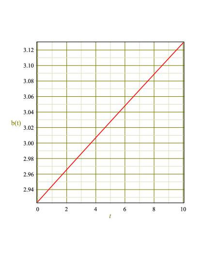
Figure 1: Graphs of scale parameter (left) and energy density (right) corresponding to $\mathrm{t}$ for minimal coupling model.

To analyze this solution, we examine the behavior of some important physical quantities such as scale factor, EoS parameter and effective matter variables that play a key role in the study of current cosmic acceleration. The EoS parameter describes distinct cosmic eras such as cosmological constant $(\omega=-1)$, phantom $(\omega<-1)$ and quintessence $(-1<\omega\leq-\frac{1}{3})$ eras. Here, we consider $m=8$ for our convenience. The graphical representation of physical quantities is the same for all even values of $m$ whereas for all odd values, we obtain the reverse behavior. The corresponding behavior of scale factor and energy density for the proposed model is shown in Figure 1. This shows that the scale parameter and energy density are positive and monotonically increasing which determines that the universe is expanding at a faster rate. Figure 2 indicates that the pressure is negatively decreasing and the EoS parameter corresponds to the quintessence era. Thus, EMSG supports the current cosmic accelerated expansion due to positively increasing behavior of the scale parameter/energy density and negatively decreasing behavior of pressure/EoS parameter.

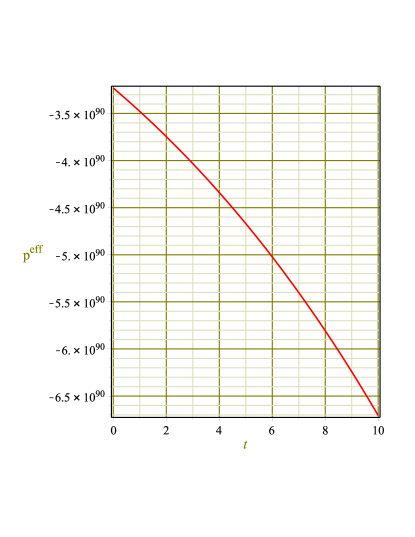
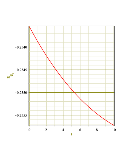
Figure 2: Graphs of pressure (left) and EoS (right) corresponding to $\mathrm{t}$ for minimal coupling model.

Case II: Non-minimal Coupling Model

This case investigates the EMSG by taking $f(\mathcal{R},\mathbf{T}^{2})=f_{0}\mathcal{R}\mathbf{T}^{2}$, where $f_{0}$ is an arbitrary constant [9]. Solving Eqs.(20)-(28), we obtain

$$\alpha=c_{2}\mathrm{b}+\frac{F_{2}(\mathrm{t})}{\sqrt{\mathrm{b}}},\quad\psi=3f_{0}\mathbf{T}^{2}\dot{F_{2}}(\mathrm{t})+F_{1}(\mathrm{t})+\dot{F_{4}}(\mathrm{t})\mathrm{b}^{\frac{3}{2}},$$

$$\gamma=-1.5\mathbf{T}^{2}c_{2}+\frac{1.33c_{3}\mathrm{b}}{f_{0}}+\frac{0.5F_{4}(\mathrm{t})}{f_{0}}+c_{1},\quad\xi=c_{3},$$

$$\rho=\frac{\sqrt{3f_{0}c_{2}\mathrm{b}^{\frac{3}{2}}\left(39c_{3}\mathrm{b}^{\frac{5}{2}}+50c_{1}f_{0}\mathrm{b}^{\frac{3}{2}}+75c_{2}c_{4}f_{0}\right)}}{15f_{0}c_{2}\mathrm{b}^{\frac{3}{2}}},\quad\beta=0.$$ (34)

The symmetry generators and corresponding conserved parameters are

$$\mathrm{K}_{2} = \mathrm{b}\frac{\partial}{\partial\mathrm{b}}-1.5\mathbf{T}^{2}\frac{\partial}{\partial\mathbf{T}^{2}},\quad\mathrm{K}_{3}=\frac{\partial}{\partial t}+\frac{1.33\mathrm{b}}{f_{0}}\frac{\partial}{\partial\mathbf{T}^{2}},$$ (35)

$$\mathcal{I}_{1} = -3f_{0}\mathrm{b}^{0.5}\dot{\mathrm{b}},\quad\mathcal{I}_{2}=-3f_{0}\mathrm{b}^{1.5}\dot{\mathbf{T}^{2}}+4.5f_{0}\mathrm{b}^{0.5}\dot{\mathrm{b}}\mathbf{T}^{2},$$ (36)

$$\mathcal{I}_{3} = -3.99\mathrm{b}^{1.5}\dot{\mathrm{b}}+3f_{0}\mathrm{b}^{0.5}\dot{\mathrm{b}}\dot{\mathbf{T}^{2}}+\mathrm{b}^{1.5}\mathcal{R}f_{0}\mathbf{T}^{2}-\mathrm{b}^{1.5}f_{0}\mathcal{R}\mathbf{T}^{2}.$$ (37)

The exact solution of the first conserved quantity is given by

$$\mathrm{b}(\mathrm{t})=\left(\mathrm{b}_{0}+\frac{\mathcal{I}_{1}\mathrm{t}}{2f_{0}}\right)^{\frac{2}{3}}.$$ (38)

This equation plays a significant role to analyze the viability of EMSG. Figure 3 shows that the energy density is positive and tends to zero as we go away from the origin whereas scale parameter is positively increasing which experiences the accelerated expansion of the universe. The negative behavior of the pressure as well as EoS parameter (Figure 4) ensure the presence of DE, which is an important candidate for cosmic acceleration.

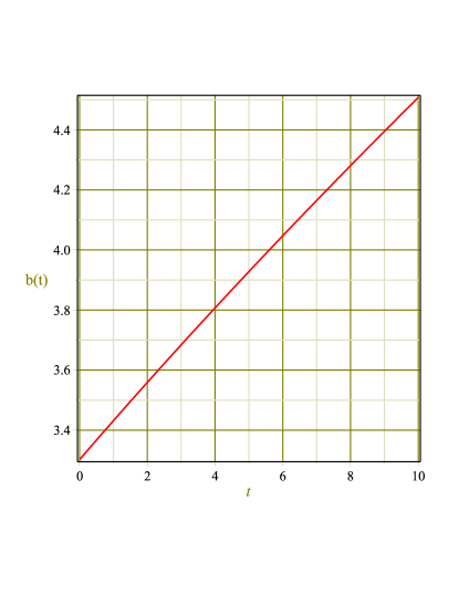
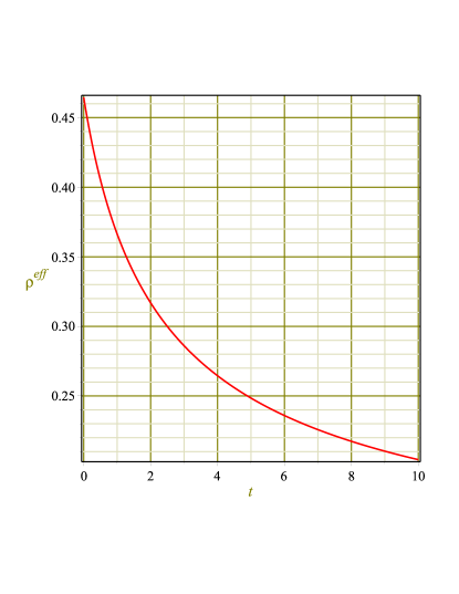
Figure 3: Graphs of scale parameter (left) and energy density (right) corresponding to $\mathrm{t}$ for non-minimal coupling model.

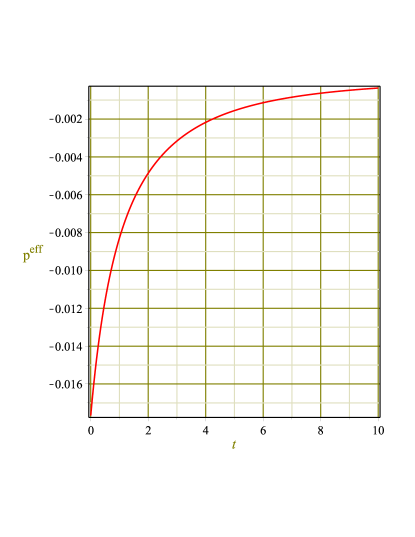
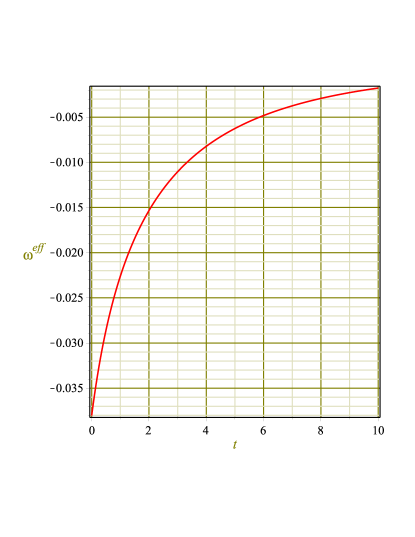
Figure 4: Graphs of pressure (left) and EoS parameter (right) corresponding to $\mathrm{t}$ for non-minimal coupling model.

Case III: $f(\mathcal{R},\mathbf{T}^{2})=f(\mathcal{R})$

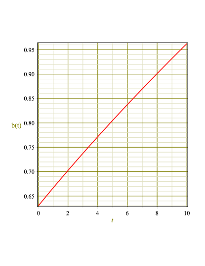
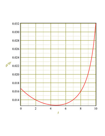
Figure 5: Graphs of scale parameter (left) and energy density (right) corresponding to $\mathrm{t}$ for $f(\mathcal{R})$ model.

Here, we choose $f(\mathcal{R},\mathbf{T}^{2})=f_{0}\mathcal{R}^{\frac{3}{2}}$ to re-analyze the $f(\mathcal{R})$ theory. This model has already been used in various papers [30] which provides viable solutions. Manipulating (20)-(28), we have

$$\alpha=c_{2}\mathrm{b}+\frac{F_{2}(\mathrm{t})}{\sqrt{\mathrm{b}}},\quad\psi=\frac{9}{2}\sqrt{\mathcal{R}}f_{0}\dot{F_{2}}(t)+F_{3}(\mathrm{t})+\dot{F_{4}}(\mathrm{t})\mathrm{b}^{\frac{3}{2}},\quad\xi=c_{1},$$

$$\beta=\frac{1.78c_{1}\sqrt{\mathcal{R}}\mathrm{b}}{f_{0}}+\frac{0.67F_{4}(\mathrm{t})\sqrt{\mathcal{R}}}{f_{0}}+(c_{3}-3\sqrt{\mathcal{R}}c_{2})\mathcal{R}^{0.5},\quad\rho=0,$$

$$\mathrm{p}=\mathrm{b}^{\frac{-3}{2}}c_{4}-f_{0}\mathcal{R}^{\frac{3}{2}}+\frac{0.534\mathrm{b}\mathcal{R}c_{1}}{c_{2}}+\frac{0.5\mathcal{R}f_{0}c_{3}}{c_{2}},\quad\gamma=0.$$ (39)

The symmetry generators can be determined as

$$\mathrm{K}_{1}=\frac{\partial}{\partial t}+\frac{1.78\mathrm{b}\sqrt{\mathcal{R}}}{f_{0}}\frac{\partial}{\partial\mathcal{R}},\quad\mathrm{K}_{2}=\mathrm{b}\frac{\partial}{\partial\mathrm{b}}-3\mathcal{R}\frac{\partial}{\partial\mathcal{R}},\quad\mathrm{K}_{3}=\sqrt{\mathcal{R}}\frac{\partial}{\partial\mathcal{R}},$$

and corresponding conserved quantities become

$$\mathcal{I}_{1} = \mathrm{b}^{1.5}f-5.340\mathrm{b}^{1.5}\dot{\mathrm{b}}\sqrt{\mathcal{R}}f_{0}^{-1}f_{\mathcal{R}\mathcal{R}}+3\mathrm{b}^{0.5}\dot{\mathrm{b}}\dot{\mathcal{R}}f_{\mathcal{R}\mathcal{R}}+\mathrm{b}^{1.5}\mathrm{p}$$ (40)

$$- \mathrm{b}^{1.5}\mathcal{R}f_{\mathcal{R}}-\mathrm{b}^{1.5}\mathbf{T}^{2}f_{\mathbf{T}^{2}}+3\mathrm{b}^{1.5}f_{\mathbf{T}^{2}}\mathrm{p}^{2}+3\mathrm{b}^{0.5}\dot{\mathrm{b}}\dot{\mathbf{T}^{2}}f_{\mathcal{R}\mathbf{T}^{2}},$$

$$\mathcal{I}_{2} = -3\mathrm{b}^{1.5}\dot{\mathcal{R}}f_{\mathcal{R}\mathcal{R}}-3\mathrm{b}^{1.5}\dot{\mathbf{T}^{2}}f_{\mathcal{R}\mathbf{T}^{2}}+9\mathrm{b}^{0.5}\dot{\mathrm{b}}\mathcal{R}f_{\mathcal{R}\mathcal{R}},$$ (41)

$$\mathcal{I}_{3} = -3\mathrm{b}^{0.5}\dot{\mathrm{b}}\mathcal{R}^{0.5}f_{\mathcal{R}\mathcal{R}}.$$ (42)

We are unable to derive an exact solution from the first and second conserved quantities $(\mathcal{I}_{1},\mathcal{I}_{2})$ due to their complicated nature. Therefore, we use

$$\mathcal{I}_{3}+3\mathrm{b}^{0.5}\dot{\mathrm{b}}\mathcal{R}^{0.5}f_{\mathcal{R}\mathcal{R}}=0,$$ (43)

where solution is

$$\mathrm{b}(\mathrm{t})=\left(\mathrm{b}_{0}+\frac{2\mathcal{I}_{3}\mathrm{t}}{3f_{0}}\right)^{\frac{2}{3}}.$$ (44)

Figure 5 indicates the behavior of energy density as positively decreasing in the initial state but with the passage of time it shows increasing behavior and $\mathrm{b}(\mathrm{t})$ as positively increasing which represents the current cosmic accelerated expansion. Figures 6 shows that pressure is negative and has decreasing trend whereas the $\omega$ corresponds to phantom era which represents the rapid cosmic expansion.

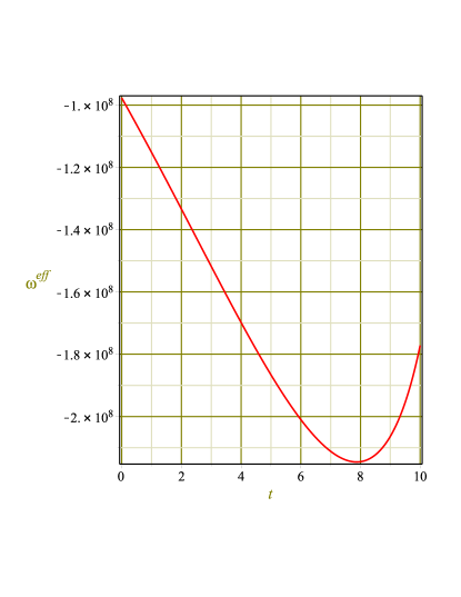
Figure 6: Graphs of pressure (left) and EoS parameter (right) corresponding to $\mathrm{t}$ for $f(\mathcal{R})$ model.

5 Final Remarks

In this paper, we have investigated exact cosmological solutions of BT-I spacetime through Noether symmetry technique in the background of EMSG. These symmetries provide solutions of the physical system and their existence yield some suitable conditions to select the cosmological models based on current observations [36]. The Lagrangian reduces the system’s complexity and helps to derive exact solutions. We have developed the Lagrangian in the context of EMSG and formulated conserved parameters to analyze analytic solutions of the field equations. The exact solutions of Noether equations have been examined for three different types of functions. The obtained results are summarized as follows.

• In the first case, we have formulated three non-zero symmetry generators and corresponding conserved parameters. The first two conserved parameters are quite complicated and it is too difficult to obtain exact solutions from these conserved quantities. The third conserved quantity provides the exact solution which is examined by analyzing the behavior of different cosmological parameters. The scale factor and energy density determine that the universe is in the accelerated expansion phase (Figure 1). The pressure and EoS parameters show negative behavior which determines the quintessence era (Figures 2).

• For the second case, the resulting solution indicates that the energy density is positive and the scale factor shows that our current universe is in the accelerated expansion phase (Figure 3). The negative behavior of the pressure describes the existence of DE whereas the EoS parameter manifests the cosmic acceleration (Figures 4).

• In the last case, the exact solution provides decreasing trend of the energy density initially but shows increasing behavior as we go away from the origin while the scale parameter is positive and has increasing behavior (Figure 5). The pressure is negatively decreasing whereas the EoS parameter corresponds to the phantom era which shows the rapid expansion of the universe (Figure 6).

It is worthwhile to mention here that for $n=1$ all the results reduce to [32]. In other modified theories of gravity, the results are consistent corresponding to particular model [37]. We conclude that all proposed models of $f(\mathcal{R},\mathbf{T}^{2})$ theory supports the current cosmic accelerated expansion.

References

• [1] Perlmutter, S. et al.: Bull. Am. Astron. Soc. 29(1997)1351; Filippenko, A.V. and Riess, A.G.: Phys. Rep. 307(1998)31; Tegmark, M. et al.: Phys. Rev. D 69(2004)103501; Spergel, D.N. et al.: Astrophys. J. Suppl. 170(2007)377.
• [2] Carroll, S.M.: Living Rev. Relativ. 4(2001)1; Sirivastava, S.K.: General Relativity and Cosmology (Prentice Hall of India, 2008).
• [3] Cognola, G. et al.: Phys. Rev. D 77(2008)046009; Felice, A.D. and Tsujikawa, S.R.: Living Rev. Relativ. 13(2010)3; Nojiri, S. and Odintsov, S.D.: Phys. Rep. 505(2011)59; Bamba, K. et al.: Astrophys. Space Sci. 342(2012)155.
• [4] Harko, T., Koivisto, T.S. and Lobo, F.S.N.: Mod. Phys. Lett. A 26(2011)1467.
• [5] Haghani, Z. et al.: Phys. Rev. D 88(2013)044023.
• [6] Katirci, N. and Kavuk, M.: Eur. Phys. J. Plus 129(2014)163.
• [7] Board, C.V.R. and Barrow, J.D.: Phys. Rev. D 96(2017)123517.
• [8] Nari, N. and Roshan, M.: Phys. Rev. D 98(2018)024031; Akarsu, O. et al.: Phys. Rev. D 97(2018)124017.
• [9] Bahamonde, S., Marciu, M. and Rudra, P.: Phys. Rev. D 100(2019)083511.
• [10] Barbar, A.H., Awad, A.M. and AlFiky, M.T.: Phys. Rev. D 101(2020)044058.
• [11] Singh, K.N. et al.: Phys. Dark Universe 31(2021)100774; Rudra, P. and Pourhassan, B.: arXiv:2008.11034v1.
• [12] Sharif, M. and Gul, M.Z.: Int. J. Mod. Phys. A 36(2021)2150004; Chin. J. Phys. 71(2021)365; Universe 07(2021)154.
• [13] Barrow, J.D. and Turner, M.S.: Nature 292(1982)35; Demianski, M.: Nature 307(1984)140.
• [14] Akarsu, O. and Kilinc, C.B.: Astrophys. Space Sci. 326(2010)315.
• [15] Yadav, A.K. and Saha, B.: Astrophys. Space Sci. 337(2012)759.
• [16] Adhav, K.S.: Astrophys. Space Sci. 339(2012)365.
• [17] Shamir, M.F.: Eur. Phys. J. C 75(2015)8.
• [18] Sharif, M. and Jabbar, S.: Commun. Theor. Phys. 63(2015)168.
• [19] Demianski, M. et al.: Phys. Rev. D 46(1992)1391.
• [20] Hanc, J., Tuleja, S. and Hancova, M.: Am. J. Phys. 72(2004)428.
• [21] Capozziello, S., Marmo, G. and Rubano, C.P.: Int. J. Mod. Phys. D 6(1997)491; Camci, U.: Eur. Phys. J. C 74(2014)3201; ibid. J. Cosmol. Astropart. Phys. 2014(2014)2.
• [22] Capozziello, S., Stabile, A. and Troisi, A.: Class. Quantum Grav. 24(2007)2153; ibid. 25(2008)085004; 27(2010)165008.
• [23] Shamir, M.F., Jhangeer, A. and Bhatti, A.A: Chin. Phys. Lett. 29(2012)080402.
• [24] Kucukakca, Y.: Eur. Phys. J. C 73(2013)2327.
• [25] Sharif, M. and Waheed, S.: J. Cosmol. Astropart. Phys. 02(2013)043.
• [26] Sharif, M. and Shafique, I.: Phys. Rev. D 90(2014)084033.
• [27] Momeni, D., Myrzakulov, R. and Gudekli, E.: Int. J. Geom. Methods Mod. Phys. 12(2015)1550101.
• [28] Sharif, M. and Fatima, H.I.: J. Exp. Theor. Phys. 122(2016)104.
• [29] Shamir, M.F. and Ahmad, M.: Eur. Phys. J. C 77(2017)55; ibid. Mod. Phys. Lett. A 32(2017)1750086.
• [30] Bahamonde, S., Bamba, K. and Camci, U.: J. Cosmol. Astropart. Phys. 02(2019)016.
• [31] Bahamonde, S., Camci, U. and Capozziello, S.: Class. Quantum Grav. 36 (2019)065013.
• [32] Sharif, M. and Gul, M.Z.: Phys. Scr. 96(2020)025002.
• [33] Sharif, M. and Gul, M.Z.: Eur. Phys. J. Plus 136(2021)503; Adv. Astron. 2021(2021)6663502.
• [34] Kantowski, R. and Sachs, R.K.: J. Math. Phys. 7(1966)443.
• [35] Xing-Xiang, W.: Chin. Phys. Lett. 22(2005)29; Bali, R. and Kumawat, P.: Phys. Lett. B 665(2008)332; Sharif, M. and Zubair, M.: Astrophys. Space Sci. 330(2010)399
• [36] Capozziello S, De Laurentis, M. and Odintsov, S.D.: Eur. Phys. J. C 72(2012)2068.
• [37] Sharif, M. and Nawazish, I.: Gen. Relativ. Gravit. 49(2017)76; Shamir, M.F. and Kanwal, F.: Eur. Phys. J. C 77(2017)1; Malik, A., Shamir, M.F. and Hussain, I.: Int. J. Geom. Methods Mod. Phys. 17(2020)2050163.