Chiral perturbation theory of the hyperfine splitting in (muonic) hydrogen

Abstract

The ongoing experimental efforts to measure the hyperfine transition in muonic hydrogen prompt an accurate evaluation of the proton-structure effects. At the leading order in $\alpha$, which is $O(\alpha^{5})$ in the hyperfine splitting (hfs), these effects are usually evaluated in a data-driven fashion, using the empirical information on the proton electromagnetic form factors and spin structure functions. Here we perform a first calculation based on the baryon chiral perturbation theory (B$\chi$PT). At leading orders it provides a prediction for the proton polarizability effects in hydrogen (H) and muonic hydrogen ($\mu$H). We find large cancellations among the various contributions leading to, within the uncertainties, a zero polarizability effect at leading order in the B$\chi$PT expansion. This result is in significant disagreement with the current data-driven evaluations. The small polarizability effect implies a smaller Zemach radius $R_{\mathrm{Z}}$, if one uses the well-known experimental $1S$ hfs in H or the $2S$ hfs in $\mu$H. We, respectively, obtain $R_{\mathrm{Z}}(\mathrm{H})=1.010(9)$ fm, $R_{\mathrm{Z}}(\mu\mathrm{H})=1.040(33)$ fm. The total proton-structure effect to the hfs at $O(\alpha^{5})$ is then consistent with previous evaluations; the discrepancy in the polarizability is compensated by the smaller Zemach radius. Our recommended value for the $1S$ hfs in $\mu\text{H}$ is $182.640(18)\,\mathrm{meV}.$

I Introduction

Muonic-atom spectroscopy has been successful at determining the charge radii of proton, deuteron, helion and alpha-particle with unprecedented precision through Lamb shift measurements [1, 2, 3]. It also holds the potential to impact tests of ab-initio nuclear theories and bound-state QED [4]. The proton Zemach radius $R_{\mathrm{Z}}$ has been extracted from a measurement of the $2S$ hyperfine splitting (hfs) in muonic hydrogen ($\mu$H) [5] with a $3.4\,\%$ uncertainty:

$$R_{\mathrm{Z}}(\mu\mathrm{H})=1.082(37)\,\mathrm{fm},$$ (1)

by comparing to the theory prediction in Ref. [6] that relies on a data-driven evaluation of the proton polarizability contribution [7]:

$$E_{\mathrm{hfs}}^{\mathrm{pol.}}(2S,\mu\text{H})=8.0(2.6)\,\upmu\mathrm{eV}.$$ (2)

Several collaborations are now preparing a measurement of the ground-state ($1S$) hfs in $\mu$H with ppm precision: CREMA [8], FAMU [9, 10] and J-PARC [11] (see Ref. [12] for a comparison of the different experimental methods). These future measurements hold the potential to extract the Zemach radius with a sub-percent uncertainty, thereby constraining the magnetic properties of the proton.

A precise theory prediction for the $1S$ hfs in $\mu$H is essential for the success of the experimental campaigns. Firstly, to narrow down the frequency search range, which is important given the limited beam time available to the collaborations at PSI, RIKEN-RAL and J-PARC. Secondly, for the interpretation of the results. One can either extract the Zemach radius given a theory prediction for the proton-polarizability effect in the $\mu$H $1S$ hfs, or vice versa, extract the proton-polarizability effect with input for the Zemach radius. Furthermore, one can combine the precise measurements of the $1S$ hfs in H and $\mu$H to disentangle the Zemach radius and polarizability effects, leveraging radiative corrections as explained in Ref. [13], and compare their empirical values to theoretical expectations.

The biggest uncertainty in the theory prediction comes from proton-structure effects, entering through the two-photon exchange (TPE). These contain the above-mentioned Zemach radius and polarizability effects. Presently, they are evaluated within a “data-driven” dispersive approach [14, 15, 16]. While the dispersive method itself is rigorous, it requires sufficient experimental data to map out the proton spin structure functions $g_{1}(x,Q^{2})$ and $g_{2}(x,Q^{2})$ as full functions of the Bjorken variable $x$ and the photon virtuality $Q^{2}$. This has been the aim of a dedicated “Spin Physics Program” at Jefferson Lab [17, 18, 19, 20, 21] that recently extended the previously scarce data for $g_{2}$ [22, 23].

In this work, we use an entirely different approach — the chiral perturbation theory ($\chi$PT) [24, 25, 26] — which has been successfully used to give a prediction for the proton-polarizability effect in the $\mu$H Lamb shift [27]. To be precise, we work in the framework of baryon chiral perturbation theory (B$\chi$PT) — the manifestly Lorentz-invariant formulation of $\chi$PT in the baryon sector [26, 28, 29] (see also [30, 31] for reviews). We show that the leading-order (LO) B$\chi$PT prediction for the polarizability effect in the hfs is effectively vanishing, thereby, in substantial disagreement with the data-driven evaluations.

The paper is organized as follows. In Sec. II, we discuss the forward TPE, and in particular, the polarizability effect in the hfs. A new formalism where one splits into contributions from the longitudinal-transverse and helicity-difference photoabsorption cross sections of the proton, $\sigma_{LT}$ and $\sigma_{TT}$, is introduced in Eq. (12). It will be shown that this decomposition is advantageous for both the dispersive, as well as the effective field theory (EFT) calculations, as it gives a cleaner access to the uncertainties. More details are given in Appendix A. In Sec. III, we present our LO B$\chi$PT prediction for the polarizability effect in the hfs of H and $\mu$H, together with a detailed discussion of the uncertainty estimate. In Sec. IV, we compare our results to data-driven dispersive and heavy baryon effective field theory (HB EFT) calculations. In Sec. V, the Zemach radius is extracted from H and $\mu$H spectroscopy based on our prediction for the polarizability effect. In Sec. VI, we discuss the TPE effect in the $\mu$H hfs in view of the forthcoming experiments. Full details of the theoretical prediction for the $1S$ $\mu$H hfs are collected in Appendix C. We finish with an outlook and conclusions.

II Two-photon exchange in the hyperfine splitting

The (muonic-)hydrogen hfs receives contributions from QED-, weak- and strong-interaction effects:

$$E_{\mathrm{hfs}}(nS)=\frac{E_{\mathrm{F}}}{n^{3}}\left(1+\Delta_{\mathrm{QED}}+\Delta_{\mathrm{weak}}+\Delta_{\mathrm{strong}}\right),$$ (3)

where the leading-order in $\alpha$ contribution is given by the Fermi energy:

$$E_{\mathrm{F}}=\frac{8Z\alpha}{3a^{3}}\frac{1+\kappa}{mM},$$ (4)

with $\alpha$ the fine-structure constant, $Z$ the charge of the nucleus (in the following $Z=1$ for the proton), $m$, $M$ the lepton and proton masses, $\kappa$ the anomalous magnetic moment of the proton, and $a^{-1}=\alpha m_{r}$ the inverse Bohr radius, with $m_{r}=mM/(m+M)$ the reduced mass. The strong-interaction effects arise from the composite structure of the proton. They begin to enter at $\mathcal{O}(\alpha^{5})$, see for instance Ref. [14], where they are split into the Zemach-radius, recoil, and polarizability contributions:

$$\Delta_{\mathrm{strong}}=\Delta_{\mathrm{Z}}+\Delta_{\mathrm{recoil}}+\Delta_{\mathrm{pol.}}\,,$$ (5)

which can all be attributed to the forward TPE shown in Fig. 1. For a first comprehensive theory summary of the Lamb shift, fine and hyperfine structure in $\mu$H, including proton-structure dependent effects, we refer to Ref. [32]. The Zemach and recoil terms ($\Delta_{\mathrm{Z}}$ and $\Delta_{\mathrm{recoil}}$) are elastic contributions with a proton in the intermediate state, see Fig. 1 (a). The diagram in Fig. 1 (b) contains excited intermediate states ($\pi N$, $\Delta$-isobar, etc.) represented by the ‘blob’. It generates the polarizability effect ($\Delta_{\mathrm{pol.}}$) that shall be evaluated in this work.

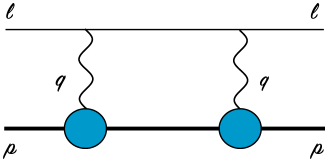
(a)

(b)

Figure 1: Two-photon-exchange diagram in forward kinematics: (a) Elastic contribution; (b) polarizability contribution. The horizontal lines correspond to the lepton and the proton (bold), where the ‘blob’ represents all possible excitations. The crossed diagrams are not drawn.

The forward TPE contribution to the hfs can be expressed through the spin-dependent forward doubly-virtual Compton scattering (VVCS) amplitudes, $S_{1}$ and $S_{2}$, cf. Eq. (41). The latter can be related to the proton structure functions $g_{1}$ and $g_{2}$ in a dispersive approach, cf. Eqs. (52) and (53). A full derivation of the well-known formalism for the TPE contribution to the hfs can be found in Appendix A.

The largest TPE effect is due to the Zemach radius contribution:

$$\Delta_{\mathrm{Z}}=-2\alpha m_{r}R_{\mathrm{Z}}.$$ (6)

The recoil contribution is one order of magnitude smaller [7], and will not be considered in this paper. It has been recently updated in Ref. [33]. The hfs is therefore best suited for a precision extraction of the Zemach radius, defined as the following integral over the electric and magnetic Sachs form factors $G_{E}(Q^{2})$ and $G_{M}(Q^{2})$ [32]:

$$R_{\mathrm{Z}}=-\frac{4}{\pi}\int_{0}^{\infty}\frac{\mathrm{d}Q}{Q^{2}}\left[\frac{G_{E}(Q^{2})G_{M}(Q^{2})}{1+\kappa}-1\right],$$ (7)

where $q^{2}=-Q^{2}$ is the photon virtuality. Equivalently, we can write:

$$R_{\mathrm{Z}}=\langle r\rangle_{E}+\langle r\rangle_{M}-\frac{2}{\pi^{2}}\int_{0}^{\infty}\frac{\mathrm{d}t}{t}\frac{\operatorname{Im}G_{M}(t)}{1+\kappa}\int_{0}^{\infty}\frac{\mathrm{d}t^{\prime}}{t^{\prime}}\frac{\operatorname{Im}G_{E}(t^{\prime})}{\sqrt{t}+\sqrt{t^{\prime}}},$$ (8)

where the linear electric and magnetic radii are defined as:

$$\langle r\rangle_{E,M}=\frac{2}{\pi}\int_{0}^{\infty}\frac{\mathrm{d}t}{t^{3/2}}\operatorname{Im}G(t),$$ (9)

with $\operatorname{Im}G(t)$ the imaginary part of the normalized electric or magnetic Sachs form factor, $G_{E,M}(Q^{2})/G_{E,M}(0)$. As one can see from Eqs. (7) and (8), a measurement of the Zemach radius gives access to the magnetic properties of the proton.

The polarizability effect in the hfs is fully constrained by empirical information on the proton spin structure functions $g_{1}(x,Q^{2})$ and $g_{2}(x,Q^{2})$, and the Pauli form factor $F_{2}(Q^{2})$, functions of $Q^{2}$ and the Bjorken variable $x=Q^{2}/2M\nu$, where $\nu$ is the photon energy in the lab frame. This is in contrast to the Lamb shift, where the knowledge of a subtraction function, $T_{1}(0,Q^{2})$ or $T_{1}(iQ,Q^{2})$ [34], is needed. It reads:

$$\Delta_{\mathrm{pol.}} =\Delta_{1}+\Delta_{2}=\frac{\alpha m}{2\pi(1+\kappa)M}\big{(}\delta_{1}+\delta_{2}\big{)},$$ (10a)

$$\delta_{1} =2\int_{0}^{\infty}\frac{\mathrm{d}Q}{Q}\left\{\frac{5+4v_{l}}{(v_{l}+1)^{2}}\Big{[}4I_{1}(Q^{2})+F_{2}^{2}(Q^{2})\Big{]}-\frac{32M^{4}}{Q^{4}}\int_{0}^{x_{0}}\mathrm{d}x\,x^{2}g_{1}(x,Q^{2})\right.$$ (10b)

$$\times\left.\frac{1}{(v_{l}+v_{x})(1+v_{x})(1+v_{l})}\left(4+\frac{1}{1+v_{x}}+\frac{1}{v_{l}+1}\right)\right\},\qquad$$

$$\delta_{2} =96M^{2}\int_{0}^{\infty}\frac{\mathrm{d}Q}{Q^{3}}\int_{0}^{x_{0}}\mathrm{d}x\,g_{2}(x,Q^{2})\left(\frac{1}{v_{l}+v_{x}}-\frac{1}{v_{l}+1}\right),$$ (10c)

with $x_{0}$ the inelastic threshold, $v_{l}=\sqrt{1+\nicefrac{{1}}{{\tau_{l}}}}$, $v_{x}=\sqrt{1+x^{2}\tau^{-1}}$, $\tau_{l}=\nicefrac{{Q^{2}}}{{4m^{2}}}$, $\tau=\nicefrac{{Q^{2}}}{{4M^{2}}}$, and the generalized Gerasimov-Drell-Hearn (GDH) integral:

$$I_{1}(Q^{2})=\frac{2M^{2}}{Q^{2}}\int_{0}^{x_{0}}\mathrm{d}x\,g_{1}(x,Q^{2})=\bar{I}_{1}(Q^{2})-F_{2}^{2}(Q^{2})/4.$$ (11)

Here, $\bar{I}_{1}$ is the polarizability part of $I_{1}$. For the origin of the Pauli form factor in the above equations, see discussion in Appendix A.

As we will show in Sec. III.2, instead of decomposing into $\Delta_{1}$ and $\Delta_{2}$, it is convenient to decompose into contributions from the longitudinal-transverse and helicity-difference cross sections $\sigma_{LT}$ and $\sigma_{TT}$:

$$\Delta_{\mathrm{pol.}}=\Delta_{LT}+\Delta_{TT}+\Delta_{F_{2}}=\frac{\alpha m}{2\pi(1+\kappa)M}\left(\delta_{LT}+\delta_{TT}+\delta_{F_{2}}\right),$$ (12a)

where we define:

$$\delta_{LT}=\frac{4M}{\alpha\pi^{2}}\int_{0}^{\infty}\!\mathrm{d}Q\int_{0}^{x_{0}}\!\mathrm{d}x\,\frac{1}{v_{l}+v_{x}}\frac{1}{x^{2}+\tau}\left[1-\frac{1}{(1+v_{l})(1+v_{x})}\right]\sigma_{LT}(x,Q^{2}),$$ (12b)

$$\delta_{TT}=\frac{4M^{2}}{\alpha\pi^{2}}\int_{0}^{\infty}\frac{\mathrm{d}Q}{Q}\int_{0}^{x_{0}}\frac{\mathrm{d}x}{x}\frac{1}{1+v_{l}}\left[\frac{2\tau}{x^{2}+\tau}+\frac{1}{(v_{l}+v_{x})(1+v_{x})}\right]\sigma_{TT}(x,Q^{2}),$$ (12c)

$$\delta_{F_{2}}=2\int_{0}^{\infty}\frac{\mathrm{d}Q}{Q}\frac{5+4v_{l}}{(v_{l}+1)^{2}}\,F_{2}^{2}(Q^{2}).$$ (12d)

Or equivalently, in terms of the VVCS amplitudes, we can write:

$$\delta_{LT} =\frac{8M}{\alpha}\frac{1}{(2\pi)^{3}}\frac{1}{i}\int_{-\infty}^{\infty}\!\mathrm{d}\nu\!\int\!\mathrm{d}\mathbf{q}\,\frac{1}{Q^{4}-4m^{2}\nu^{2}}\left\{\bar{S}_{1}(\nu,Q^{2})+\frac{\nu}{M}\bar{S}_{2}(\nu,Q^{2})\right\}$$

$$-\frac{2}{m^{2}}\int_{0}^{\infty}\mathrm{d}Q\,Q\,(v_{l}-1)\,F_{2}^{2}(Q^{2}),$$ (13a)

$$\delta_{TT} =\frac{4M}{\alpha}\frac{1}{(2\pi)^{3}}\frac{1}{i}\int_{-\infty}^{\infty}\!\mathrm{d}\nu\!\int\!\mathrm{d}\mathbf{q}\,\frac{1}{Q^{4}-4m^{2}\nu^{2}}\left\{\frac{\nu}{M}\bar{S}_{2}(\nu,Q^{2})-\frac{\nu^{2}}{Q^{2}}\bar{S}_{1}(\nu,Q^{2})\right\}$$

$$-2\int_{0}^{\infty}\frac{\mathrm{d}Q}{Q}\frac{1}{(v_{l}+1)^{2}}\,F_{2}^{2}(Q^{2}).$$ (13b)

Here, $\bar{S}_{i}$ denotes the non-Born part of the amplitudes. An advantage of the B$\chi$PT calculation in this work is that the non-Born amplitudes can be calculated directly, and need not be constructed through the dispersive formalism. Furthermore, at the present order of our calculation in the B$\chi$PT power counting, there are no contributions to the elastic form factors, and thus, $I_{1}$ in Eq. (11) is given by the polarizability part only.

III Chiral loops

Assuming B$\chi$PT is an adequate theory of low-energy nucleon structure, it should be well applicable to atomic systems, where the relevant energies are naturally small. In Ref. [27], the polarizability effect in the $\mu$H Lamb shift has been successfully predicted at LO in B$\chi$PT. Here, we extend this calculation to the polarizability effect in the hfs. This requires the spin-dependent non-Born VVCS amplitudes, $\bar{S}_{1}$ and $\bar{S}_{2}$, at chiral $\mathcal{O}(p^{3})$ in the B$\chi$PT power counting.

Figure 1 in Ref. [27] shows the leading polarizability effect given by the TPE diagrams of elastic lepton-proton scattering with one-loop $\pi N$ insertions. For the Compton-like processes, it is convenient to use the chirally-rotated leading B$\chi$PT Lagrangian for the pion $\pi^{a}(x)$ and nucleon $N(x)$ fields [38]:

$$\mathcal{L}_{\pi N}^{(1)} = \bar{N}\Big{(}i\not{\partial}-M_{N}-i\frac{g_{A}}{f_{\pi}}M_{N}\tau^{a}\pi^{a}\gamma_{5}+\frac{g_{A}^{2}}{2f_{\pi}^{2}}M_{N}\pi^{2}+\frac{g_{A}^{2}-1}{4f_{\pi}^{2}}\tau^{a}\epsilon^{abc}\pi^{b}\not{\partial}\,\pi^{c}\Big{)}N+\mathcal{O}(\pi^{3}),$$ (14)

where $\gamma_{5}=i\gamma^{0}\gamma^{1}\gamma^{2}\gamma^{3}$, $g_{A}\simeq 1.27$ [39] is the axial coupling of the nucleon, $f_{\pi}\simeq 92.21$ MeV is the pion-decay constant, $\tau^{a}$ are the Pauli matrices, $M_{N}\simeq 938.27$ MeV and $m_{\pi}\simeq 139.57$ MeV are the nucleon and pion masses. As described in Ref. [27], the Born part is separated from the $\mathcal{O}(p^{3})$ VVCS amplitudes by subtracting the on-shell pion-loop $\gamma NN$-vertex in the one-particle-reducible VVCS graphs, see diagrams (b) and (c) in Figure 1 of Ref. [27]. For more details on the B$\chi$PT framework, we refer to Refs. [40, 41, 42], where the complete next-to-next-to-leading-order (NNLO) in the $\delta$-expansion [43] B$\chi$PT calculation of the spin-independent and spin-dependent nucleon VVCS amplitudes can be found.

In practice, most results here were obtained based on our B$\chi$PT prediction for the $\pi N$-production channel in the structure functions $g_{i}$, given in Ref. [42, Appendix B]. It has been verified that the results agree with the calculation based on the VVCS amplitudes $\bar{S}_{i}$.

III.1 Numerical results

Our LO B$\chi$PT prediction for the polarizability effect in the $1S$ hfs of H and $\mu$H amounts to:

$$E_{\mathrm{hfs}}^{{\langle\mathrm{LO}\rangle}\,\mathrm{pol.}}(1S,\mathrm{H}) = 0.69(2.03)\,\mathrm{peV},$$ (15a)

$$E_{\mathrm{hfs}}^{{\langle\mathrm{LO}\rangle}\,\mathrm{pol.}}(1S,\mu\mathrm{H}) = 6.8(11.4)\,\upmu\mathrm{eV}.$$ (15b)

The error estimate will be described and motivated in the subsequent sections. The corresponding contributions to the $nS$ hfs are trivially obtained through a $1/n^{3}$ scaling, as can be seen from Eqs. (3) and (4). Splitting into contributions from the spin structure functions $g_{1}$ and $g_{2}$, we obtain:

$$E_{\mathrm{hfs}}^{{\langle\mathrm{LO}\rangle}\,\mathrm{pol.}}(1S,\mathrm{H},\Delta_{1}) = 0.3(3.1)\,\mathrm{peV},\qquad E_{\mathrm{hfs}}^{{\langle\mathrm{LO}\rangle}\,\mathrm{pol.}}(1S,\mathrm{H},\Delta_{2})=0.4(1.0)\,\mathrm{peV},$$ (16a)

$$E_{\mathrm{hfs}}^{{\langle\mathrm{LO}\rangle}\,\mathrm{pol.}}(1S,\mu\mathrm{H},\Delta_{1}) = 5.2(16.5)\,\upmu\mathrm{eV},\qquad E_{\mathrm{hfs}}^{{\langle\mathrm{LO}\rangle}\,\mathrm{pol.}}(1S,\mu\mathrm{H},\Delta_{2})=1.6(5.2)\,\upmu\mathrm{eV}.$$ (16b)

Strikingly, the contributions from the longitudinal-transverse and helicity-difference cross sections $$\sigma_{LT} \sigma_{TT}$$ and :

$$E_{\mathrm{hfs}}^{{\langle\mathrm{LO}\rangle}\,\mathrm{pol.}}(1S,\mathrm{H},\Delta_{LT}) = 5.1(1.5)\,\mathrm{peV},\qquad E_{\mathrm{hfs}}^{{\langle\mathrm{LO}\rangle}\,\mathrm{pol.}}(1S,\mathrm{H},\Delta_{TT})=-4.4(1.3)\,\mathrm{peV},$$ (16c)

$$E_{\mathrm{hfs}}^{{\langle\mathrm{LO}\rangle}\,\mathrm{pol.}}(1S,\mu\mathrm{H},\Delta_{LT}) = 30.0(9.0)\,\upmu\mathrm{eV},\qquad E_{\mathrm{hfs}}^{{\langle\mathrm{LO}\rangle}\,\mathrm{pol.}}(1S,\mu\mathrm{H},\Delta_{TT})=-23.2(7.0)\,\upmu\mathrm{eV},$$ (16d)

are one order of magnitude larger than the total, and differ in their respective signs. This indicates a cancellation of LO contributions between $\Delta_{LT}$ and $\Delta_{TT}$.

Including in addition the correction due to electron vacuum polarization (eVP) in the TPE diagram, see Fig. 10 and discussion in Appendix B, gives a negligible effect within the present uncertainties:

$$E_{\mathrm{hfs}}^{{\langle\mathrm{LO}\rangle}\,\text{pol. + eVP}}(1S,\mathrm{H}) = 0.72(2.07)\,\mathrm{peV},$$ (17a)

$$E_{\mathrm{hfs}}^{{\langle\mathrm{LO}\rangle}\,\text{pol. + eVP}}(1S,\mu\mathrm{H}) = 7.0(11.6)\,\upmu\mathrm{eV}.$$ (17b)

Nevertheless, it is important in view of the anticipated $1$ ppm accuracy (corresponding to $\sim 0.2\,\upmu$eV) of the $\mu$H $1S$ hfs measurement by the CREMA collaboration [8]. We therefore include the additional $\Delta_{\mathrm{pol.}}^{\mathrm{eVP}}(\text{H})=0.01$ ppm and $\Delta_{\mathrm{pol.}}^{\mathrm{eVP}}(\mu\text{H})=1$ ppm on top of $\Delta_{\mathrm{pol.}}(\text{H})=0.12(35)$ ppm and $\Delta_{\mathrm{pol.}}(\mu\text{H})=37(62)$ ppm.

To understand why the contributions from $\sigma_{LT}$ and $\sigma_{TT}$ largely cancel in $\Delta_{\mathrm{pol.}}$, we study the heavy-baryon (HB) limit of the spin-dependent VVCS amplitudes [48]. Expanding the LO B$\chi$PT expression for the $\bar{S}_{1}$ amplitude in $\mu=m_{\pi}/M_{N}$ while keeping the ratio of the light scales $\tau_{\pi}=\nicefrac{{Q^{2}}}{{4m_{\pi}^{2}}}$ fixed, one obtains:

$$\bar{S}_{1}(0,Q^{2})\!\stackrel{{\scriptstyle\text{HB}}}{{=}}\!-\frac{3\,\alpha\,g_{A}^{2}}{16f_{\pi}^{2}}\,m_{\pi}\!\left[1-(1+\tau_{\pi})\frac{\arctan\sqrt{\tau_{\pi}}}{\sqrt{\tau_{\pi}}}\right]\!.$$ (18)

We then take a closer look at the first term in the low-energy polarizability expansion:

$$\frac{\bar{S}_{1}(0,Q^{2})}{Q^{2}}\Big{|}_{Q^{2}\rightarrow 0}=M_{N}\left\{\gamma_{E1M2}-3\alpha M_{N}\left[P^{\prime(M1,M1)1}(0)+P^{\prime(L1,L1)1}(0)\right]\right\}.$$ (19)

The HB$\chi$PT predictions for the proton polarizabilities [49, 50, 51, 52, 53, 54] entering Eq. (19) read:

$$\gamma_{E1M2} = \frac{\alpha g_{A}^{2}}{(4\pi f_{\pi})^{2}}\frac{1}{m_{\pi}^{2}}\frac{1}{6}\left[1-\frac{7\pi}{4}\frac{m_{\pi}}{M_{N}}\right]\!,$$ (20a)

$$P^{\prime(M1,M1)1}(0) = \frac{g_{A}^{2}}{(4\pi f_{\pi})^{2}}\frac{1}{m_{\pi}^{2}}\frac{1}{18M}\left[-1+\frac{7\pi}{4}\frac{m_{\pi}}{M_{N}}\right]\!,$$ (20b)

$$P^{\prime(L1,L1)1}(0) = \frac{g_{A}^{2}}{(4\pi f_{\pi})^{2}}\frac{1}{m_{\pi}^{2}}\frac{1}{9M}\left[1-\frac{17\pi}{8}\frac{m_{\pi}}{M_{N}}\right]\!.$$ (20c)

We can see that the leading terms in the chiral expansion are of $\mathcal{O}(1/m_{\pi}^{2})$. They cancel among the different polarizabilities, thus, Eq. (21) becomes a subleading contribution:

$$\frac{\bar{S}_{1}(0,Q^{2})}{Q^{2}}\Big{|}_{Q^{2}\rightarrow 0}\stackrel{{\scriptstyle\text{HB}}}{{=}}\frac{\alpha g_{A}^{2}}{32f_{\pi}^{2}}\frac{1}{m_{\pi}}.$$ (21)

Accordingly, one would expect the chiral loops in the hfs to be small. Indeed, the LO B$\chi$PT prediction in Eq. (15) is essentially vanishing, where the small number is mainly a remnant of higher orders in the HB expansion. This has to be taken into account in the uncertainty estimate.

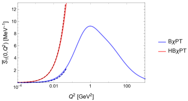
Figure 2: The amplitude $\bar{S}_{1}(0,Q^{2})$ at LO in B$\chi$PT (blue) and HB$\chi$PT (red). The dashed lines show the corresponding slope terms, i.e., the first terms in the expansion in powers of $Q^{2}$. The B$\chi$PT slope has been calculated from the polarizabilities given in Ref. [55, Table I], the HB$\chi$PT slope is given in Eq. (21).

Note that the HB expansion above has been introduced for instructive purposes only, but is not entering our calculation of the polarizability effect. The HB$\chi$PT prediction of the $S_{1}(0,Q^{2})$ amplitude, Eq. (18), raises with $Q$, thus, its contribution to the hfs will be divergent. This can be seen from Fig. 2, where we compare the chiral-loop contribution to $\bar{S}_{1}(0,Q^{2})$ as predicted by B$\chi$PT and HB$\chi$PT, respectively.

III.2 Uncertainty estimate

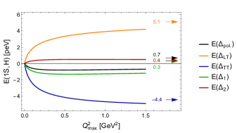
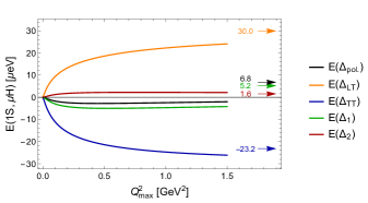
Figure 3: Polarizability effect on the $1S$ hyperfine splitting in H (left panel) and $\mu$H (right panel): Cutoff dependence of the leading-order $\pi N$-loop contribution. The total results, Eqs. (15a) and (15b), are indicated by the black arrows.

B$\chi$PT is a low-energy EFT of QCD describing strong interactions in terms of hadronic degrees of freedom (pion, nucleon, $\Delta(1232)$ resonance). An important requirement for a reliable B$\chi$PT prediction is that the contribution from beyond the scale at which this EFT is safely applicable, i.e., $Q_{\mathrm{max}}>m_{\rho}=775$ MeV, has to be small. For the LO B$\chi$PT prediction of the polarizability effect in the $\mu$H Lamb shift [27], the contribution from beyond this scale was less than $15\,\%$, thus, within the expected uncertainty. Comparing the TPE master formulas for Lamb shift and hfs, Eqs. (49) and (48), the weighting function in the former has a stronger suppression for large $Q^{2}$. It is therefore important to verify that the same quality criterion still holds for the hfs prediction presented here.

Let us consider the polarizability effect as a running integral with momentum cutoff $Q_{\mathrm{max}}$, as shown in Fig. 3. The convergence of the $\Delta_{1}$ (green line) contribution, as well as of the total $\Delta_{\mathrm{pol.}}$ (black line), is poor. They display a sign change of the running integral at energies above $Q_{\mathrm{max}}\approx 2$ GeV ($\mu\mathrm{H}$) and $\approx 4$ GeV ($\mathrm{H}$), respectively. $\Delta_{2}$ (red line) converges better. Its contributions from above $Q_{\mathrm{max}}=m_{\rho}$ amount to $42\,\%$ (H) and $26\,\%$ ($\mu\mathrm{H}$), respectively.

The bad high-momentum asymptotics indicated above are merely an artefact of the conventional splitting into $\Delta_{1}$ and $\Delta_{2}$. For the alternative splitting into $\Delta_{LT}$ and $\Delta_{TT}$, introduced in Eq. (12), the cut-off dependence improves considerably. For $\Delta_{TT}$ (blue line), the contribution from above $Q_{\mathrm{max}}=m_{\rho}$ amounts to less than $4\,\%$ for both hydrogens. For $\Delta_{LT}$ (orange line), the high-energy contributions are less than $35\,\%$ ($\mu\mathrm{H}$) and $32\,\%$ ($\mathrm{H}$), respectively. In this way, our results are in agreement with the natural expectation of uncertainty for a LO prediction, $30\,\%$ [$\simeq(M_{\Delta}-M)/\mathrm{GeV}$], in B$\chi$PT with inclusion of the $\Delta$ resonance. Based on this analysis, we decided to assign errors of $30\,\%$ to the $\sigma_{LT}$ and $\sigma_{TT}$ contributions, and propagate them to $\Delta_{1}$, $\Delta_{2}$ and $\Delta_{\mathrm{pol.}}$. It is interesting to note that in this way the uncertainty of $\Delta_{1}$ is larger than the uncertainty of $\Delta_{\mathrm{pol.}}$. This can be understood from the opposite signs of the $\Delta_{i,j}$ contributions, where $i=1,2$ and $j=LT,TT$, on the example of $\mu$H:

$$\Delta_{1,\,LT}= 227\,\text{ppm},\qquad\Delta_{1,\,TT} =-198\,\text{ppm},$$ (22a)

$$\qquad\Delta_{2,\,LT}= -62\,\text{ppm},\qquad\Delta_{2,\,TT} =71\,\text{ppm}.$$ (22b)

IV Comparison with other results

In this section, we compare our LO B$\chi$PT prediction for the polarizability effect in the $\mathrm{H}$ and $\mu\mathrm{H}$ hfs to other available evaluations. Furthermore, we study the contribution of the $\bar{S}_{1}(0,Q^{2})$ subtraction function and the scaling of the polarizability effect with the lepton mass.

IV.1 Heavy-baryon effective field theory

Let us start by comparing our B$\chi$PT prediction to other model-independent calculations using HB EFT [56, 57, 58]. First results for the elastic and inelastic TPE effects on the hfs in H and $\mu\mathrm{H}$ have been obtained in Ref. [56], where the contribution of the leading chiral logarithms, $\mathcal{O}(m^{3}\alpha^{5}/M^{2}\times\left[\ln m_{\pi},\ln\Delta,\ln m\right])$, was calculated in HB EFT matched to potential NRQED. At this order in the chiral expansion the polarizability effects in the hfs from pion-nucleon and pion-delta loops cancel each other in the large-$N_{c}$ limit, while the $\Delta$ exchange cancels part of the point-like corrections, see also Ref. [48]. The analytical results presented in Ref. [56, 59] motivate the relative size of the Zemach and polarizability corrections.

Updated HB EFT predictions for the TPE effects on the hydrogen spectra can be found in Refs. [57, 60, 58]. In Ref. [58], the difference between the pion-loop polarizability contributions in $\mathrm{H}$ and $\mu\mathrm{H}$ is quoted as

$$\Delta c_{4}\equiv c_{4,\mathrm{pol}}^{\mu\mathrm{H}}-c_{4,\mathrm{pol}}^{\mathrm{H}}=0.17(9),\;$$ (23)

where $c_{4}$ is a Wilson coefficient linked to the hfs in the following way:

$$E_{\mathrm{hfs}}(nS)=\frac{E_{\mathrm{F}}}{n^{3}}\frac{3\alpha}{2\pi(1+\kappa)}\frac{m}{M}\,c_{4}.$$ (24)

For comparison, we can evaluate the analogue of $\Delta c_{4}$ from other theory predictions for the polarizability contribution. Within errors, our LO B$\chi$PT prediction agrees with this result:

$$\Delta c_{4}=0.09(0.46).$$ (25)

Here, the uncertainties of the H and $\mu$H predictions have been combined in quadrature to estimate the error on their difference. For comparison, from the data-driven dispersive evaluations of Carlson et al. [14], one can deduce:

$$\Delta c_{4}=-0.27(1.53),$$ (26)

where we combined all errors quoted in Ref. [14] and estimated the error on $\Delta c_{4}$ in the same way as done above.

IV.2 Data-driven dispersive evaluations

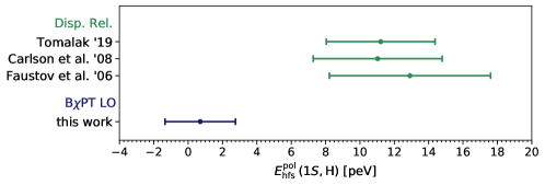
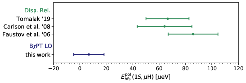
Figure 4: Comparison of available results for the polarizability effect on the hyperfine splitting in H and $\mu$H (upper and lower panel) [14, 15, 16].

There is a clear discrepancy between the B$\chi$PT prediction, presented here, and the conventional data-driven dispersive evaluations. The dispersive evaluations rely on empirical information for the inelastic proton spin structure functions, the elastic Pauli form factor and polarizabilities. The discrepancy can be seen from Fig. 4, where our LO B$\chi$PT prediction for the polarizability effect in the $\mathrm{H}$ and $\mu\mathrm{H}$ hfs is compared to the available dispersive evaluations. Adding an estimate for the next-to-leading-order (NLO) effect of the $\Delta(1232)$ resonance [61], obtained from large-$N_{c}$ relations for the nucleon-to-delta transition form factors, to the model-independent LO B$\chi$PT prediction will improve agreement for $\Delta_{2}$ but not for $\Delta_{\mathrm{pol}}$.

The origin of this discrepancy has to be understood in order to give a reliable prediction of the TPE effect in the $\mu$H hfs, needed for the forthcoming experiments. Part of the discrepancy might be due to underestimated uncertainties. An evaluation of the total polarizability effect suffers from cancellations in two places: firstly, between contributions from the cross sections $\sigma_{LT}$ and $\sigma_{TT}$, secondly, between the elastic Pauli form factor $F_{2}$ and the inelastic structure functions in the low-$Q$ region. Each of these cancellations reduces the result by an order of magnitude. In the calculation presented here, the former is taken into account by estimating the uncertainty due to higher-order corrections in the B$\chi$PT power counting based on the large $\sigma_{LT}$ and $\sigma_{TT}$ contributions, see discussion in Sec. III.2. In the dispersive approach, it would be important to take into account correlations between parametrizations of the $g_{1}$ and $g_{2}$ structure functions, which both rely on measurements of $\sigma_{LT}$ and $\sigma_{TT}$. The latter cancellations in the low-$Q$ region will be discussed in the following subsection.

IV.3 Low-$Q$ region and contribution of the $\bar{S}_{1}(0,Q^{2})$ subtraction function

One major drawback of the data-driven dispersive evaluations is that they require independent input for the inelastic spin structure functions or related polarizabilities, and the elastic Pauli form factor. Our notation in Eq. (10b) conveniently illustrates how the zeroth moment of the inelastic spin structure function $g_{1}$ and the elastic Pauli form factor $F_{2}$ combine in the subtraction function:

$$\bar{S}_{1}(0,Q^{2})=\frac{2\pi\alpha}{M}\left[F_{2}^{2}(Q^{2})+4I_{1}(Q^{2})\right]=\frac{8\pi\alpha}{M}\bar{I}_{1}(Q^{2}).$$ (27)

At $Q^{2}=0$, this is zero, because the Pauli form factor, $F_{2}(0)=\kappa$, and the generalized GDH integral, $I_{1}(0)=-\kappa^{2}/4$, so the two terms cancel exactly. A NLO B$\chi$PT prediction of the slope amounts to: $[\overline{I}_{1}]^{\prime}(0)=0.39(4)\,\mathrm{GeV}^{-2}$ [42]. It can be expressed through a combination of lowest-order spin [$\gamma_{E1M2}$] and generalized polarizabilities [$P^{\prime(M1,M1)1}(0)$ and $P^{\prime(L1,L1)1}(0)$], see Eq. (19). In the HB$\chi$PT expansion, we showed that the leading $\mathcal{O}(\nicefrac{{1}}{{m_{\pi}^{2}}})$ terms cancel among these individual polarizabilities, given in Eq. (20), turning the result subleading in $\mathcal{O}(\nicefrac{{1}}{{m_{\pi}}})$, see Eq. (21). We can conclude that there is a strong cancellation between the elastic and inelastic contributions, which continues for higher $Q^{2}$.

The contribution of $\bar{S}_{1}(0,Q^{2})$ to the hfs is given by:

$$E_{\mathrm{hfs}}^{\langle\bar{S}_{1}(0,Q^{2})\rangle}(nS)=\frac{E_{\mathrm{F}}}{n^{3}}\frac{\alpha m}{\pi(1+\kappa)M}\int_{0}^{\infty}\frac{\mathrm{d}Q}{Q}\frac{5+4v_{l}}{(v_{l}+1)^{2}}\left[4I_{1}(Q^{2})+F_{2}^{2}(Q^{2})\right].\qquad$$ (28)

Evaluations of this subtraction function contribution with empirical parametrizations for $g_{1}(x,Q^{2})$ and $F_{2}(Q^{2})$ tend towards larger values than the LO B$\chi$PT prediction. A partial calculation of the TPE effect at NLO in B$\chi$PT, considering only the one-loop box diagram with intermediate $\Delta(1232)$-excitation, will lower the theoretical prediction for the polarizability contribution from B$\chi$PT further, and in fact, turn it into a negative contribution [61, 62]. Any imprecision in the empirical parametrizations, and thus in the cancellation between the elastic and inelastic moments, is enhanced by the $1/Q$ prefactor in the infrared region of the integral in Eq. (28). Therefore, the B$\chi$PT calculation, where the polarizability effect can be accessed directly through the non-Born part of the VVCS amplitudes and does not rely on input from separate measurements, has a clear advantage in this regard.

To illustrate this further, we reproduce the estimate for $\Delta_{1}$ in the low-$Q$ region from Ref. [14] (see references therein for the details on the input). In this region, no experimental data from EG1 [63, 64] exist and the integral is completed by interpolating data between higher $Q^{2}$ and $Q^{2}=0$, making use of empirical values for the static polarizabilities. For $Q^{2}\in\left\{0,Q_{\mathrm{max}}^{2}\right\}$ with $Q_{\mathrm{max}}^{2}=0.0452\,\mathrm{GeV}^{2}$, the approximate formulas read [14]:

$$\delta_{1}(\text{H}) \sim \left(\underbrace{-\frac{3}{4}\kappa^{2}r_{\mathrm{Pauli}}^{2}}_{\rightarrow\,-2.19}+\underbrace{18M^{2}c_{1B}}_{\rightarrow\,3.54}\right)Q_{\mathrm{max}}^{2}=1.35(90),$$ (29a)

$$\delta_{1}(\mu\text{H}) \sim \left[\underbrace{-\frac{1}{3}\kappa^{2}r_{\mathrm{Pauli}}^{2}}_{\rightarrow\,-1.45}+\underbrace{8M^{2}c_{1}}_{\rightarrow\,2.13}\underbrace{-\frac{M^{2}}{3\alpha}\gamma_{0}}_{\rightarrow\,0.18}\right]\int_{0}^{Q_{\mathrm{max}}^{2}}\mathrm{d}Q^{2}\beta_{1}(\tau_{\mu})=0.86(69),$$ (29b)

where

$$\beta_{1}(\tau_{\mu})=-3\tau_{\mu}+2\tau_{\mu}^{2}+2(2-\tau_{\mu})\sqrt{\tau_{\mu}(\tau_{\mu}+1)}.$$ (30)

Note that the formulas for H and $\mu$H differ, because one sets $m_{e}=0$. The first terms are related to the elastic Pauli form factor, where $r_{\mathrm{Pauli}}=-\nicefrac{{6}}{{\kappa}}\,\nicefrac{{\mathrm{d}}}{{\mathrm{d}Q^{2}}}\,F_{2}(Q^{2})|_{Q^{2}=0}$ is the Pauli radius. The other terms are related to the $g_{1}$ contribution. Considering the more general Eq. (29b), they are defined through:

$$I_{1}(Q^{2}) = M\int_{\nu_{0}}^{\infty}\frac{\mathrm{d}\nu}{\nu^{2}}\,g_{1}(\nu,Q^{2})=-\kappa^{2}/4+2M^{2}c_{1}Q^{2}+\mathcal{O}(Q^{4}),$$ (31a)

$$\gamma_{0} = \frac{2\alpha}{M}\int_{\nu_{0}}^{\infty}\frac{\mathrm{d}\nu}{\nu^{4}}\,g_{1}(\nu,0).$$ (31b)

The strong cancellation between elastic and inelastic contributions, observed in Eq. (29), can be a source of uncertainty.

In addition, the quality of the low-$Q$ approximation is rather poor. We can test it at LO in B$\chi$PT. Recall that at this order in the B$\chi$PT power counting, there is no contribution to the elastic form factors. Therefore, only the inelastic structure function $g_{1}$ enters. Our results are shown in Fig. 5. The approximate formulas in Eq. (29) give a $50\,\%$ ($67\,\%$) larger value for $\delta_{1}$ in the region of $Q^{2}<0.0452$ GeV² in the case of $\mu$H (H). Therefore, in the data-driven dispersive approach one has to properly account for the uncertainty introduced by the approximate formulas, as well as from cancellations between elastic and inelastic contributions.

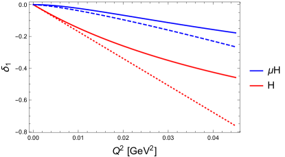
Figure 5: The polarizability contribution $\delta_{1}$ in the low-$Q$ region for hydrogen (red) and muonic hydrogen (blue). The solid lines are the exact results according to Eq. (10b) with an upper cut on the $Q$ integration. The dotted and dashed lines are evaluated with the approximate formulas for hydrogen and muonic hydrogen, respectively, see Eq. (29).

IV.4 Scaling with lepton mass

It is customary to use the high-precision measurement of the $1S$ hfs in H [65, 66]:

$$E^{\,\text{exp.}}_{1S\text{-hfs}}(\mathrm{H}) = 1\,420.405\,751\,768(1)\,\text{MHz},$$ (32)

to refine the prediction of the TPE in the $\mu$H hfs [58, 16] or the prediction of the total $\mu$H hfs [13]. We will do the same in Sec. VI. The strategies in Refs. [58, 16, 13] are slightly different, but all make statements about the scaling of various contributions to the hfs in a hydrogen-like atom when varying the lepton mass $m_{\ell}$.

In Fig. 6, we study the scaling of the polarizability effect based on our LO B$\chi$PT prediction. In the left panel, we assume that the $\Delta_{i}$ (with $i=1,2,LT,TT$ and pol.) are scaling with the reduced mass $m_{r}$. In the right panel we assume that the $\delta_{i}$ are independent of the lepton mass, thus, $\Delta_{i}$ would be scaling with $m_{\ell}$. The curves in the upper (lower) panel are normalized for H ($\mu$H), so they are fixed to $1$ at $m_{\ell}=m_{e}$ ($m_{\ell}=m_{\mu}$). If the polarizability effect would scale according to our assumptions, i.e., $\propto m_{r}$ or $\propto m_{\ell}$, all curves would be constantly $1$. We can see that the scaling works best for the contributions from $\sigma_{LT}$ and $\sigma_{TT}$, which are large in their absolute values. Considering the total, in which the contributions from $\sigma_{LT}$ and $\sigma_{TT}$ cancel by about one order of magnitude, the scaling violation is enhanced by about one order of magnitude in relative terms. The same enhancement of the scaling violation can be observed for the numerically small contributions from $g_{1}$ and $g_{2}$. Comparing left and right panels, the B$\chi$PT predictions seems to support the assumption that $\Delta_{LT}$ and $\Delta_{TT}$ are scaling with $m_{r}$. For $\Delta_{LT}$, the scaling is nearly perfect. For $\Delta_{TT}$, we observe a violation of the scaling that is increasing with lepton mass. The approximation $\Delta_{TT}(\mu\text{H})\sim m_{r}(\mu\text{H})/m_{r}(\text{H})\,\Delta_{TT}(\mu\text{H})$ holds at the level of $10\%$. The approximation holds on a similar level after including an estimate for the NLO effect of the $\Delta(1232)$ resonance [61].

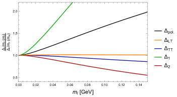
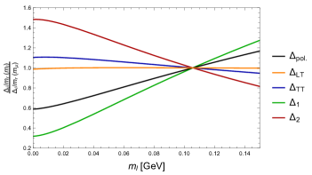
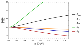
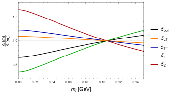
Figure 6: Scaling of $\delta_{i}$ and $\Delta_{i}/m_{r}$ (with $i=1,2,LT,TT$ and pol.), as a function of the lepton mass $m_{\ell}$.

V Extraction of the Zemach radius from spectroscopy

The TPE, entering the hfs, can be decomposed into Zemach radius, polarizability and recoil contributions, as described in Eq. (5). On top of the $\mathcal{O}(\alpha^{5})$ TPE, we consider the leading radiative corrections given by eVP, see Fig. 10 and discussion in Appendix B. Our prediction for the polarizability effect in the hfs, which is smaller than the conventional results from data-driven dispersive evaluations, also implies a smaller proton Zemach radius as previously determined from spectroscopy, cf. Eq. (1). In the following, we will extract the Zemach radius from the precisley measured $1S$ hfs in H, see Eq. (32), and the $2S$ hfs in $\mu$H [5]:

$$E^{\,\text{exp.}}_{\text{HFS}}(2S,\mu\mathrm{H})=22.8089(51)\,\text{meV}.$$ (33)

We use the theory predictions for the $1S$ hfs in H [13]:

$$E_{\text{hfs}}(1S,\text{H}) = \Big{[}1\,420\,453.106(10)\underbrace{-54.430(7)\,\left(\frac{R_{\mathrm{Z}}}{\text{fm}}\right)+E_{\mathrm{F}}\,\Big{(}0.99807(13)\,\Delta_{\mathrm{recoil}}+1.00002\,\Delta_{\mathrm{pol.}}\Big{)}}_{\text{TPE including radiative corrections}}\Big{]}\,\text{kHz}$$ (34)

and the $2S$ hfs in $\mu$H [13]:

$$E_{\text{hfs}}(2S,\mu\text{H})=\Big{[}22.9584(8)\underbrace{-0.16319(2)\left(\frac{R_{\mathrm{Z}}}{\text{fm}}\right)+\frac{E_{\mathrm{F}}}{8}\,\Big{(}1.01580(4)\,\Delta_{\mathrm{recoil}}+1.00326\,\Delta_{\mathrm{pol.}}\Big{)}}_{\text{TPE including radiative corrections}}\Big{]}\,\text{meV},$$ (35)

with the recently re-evaluated $\mathcal{O}(\alpha^{5})$ recoil correction [33]:

$$\Delta_{\mathrm{recoil}}(\mathrm{H}) = 5.269\,{}^{+0.017}_{-0.004}\;\text{ppm},$$ (36a)

$$\Delta_{\mathrm{recoil}}(\mu\mathrm{H}) = 837.6\,{}^{+2.8}_{-1.0}\;\text{ppm},$$ (36b)

up to a factor $3$ more precise than the previous best determination [67] based on the electromagnetic form factors obtained from dispersion theory [68]. An itemized list of contributions to the $2S$ hfs in $\mu$H is given in Table 3 of Appendix C. From the LO B$\chi$PT prediction for the polarizability effect, including also the eVP in Eq. (17), we obtain:

$$R_{\mathrm{Z}}(\mathrm{H}) = 1.010(9)\,\mathrm{fm},$$ (37a)

$$R_{\mathrm{Z}}(\mu\mathrm{H}) = 1.040(33)\,\mathrm{fm}.$$ (37b)

This can be compared to other determinations of the proton Zemach radius collected in Table 1. The radii we find are in agreement with the proton form factor analysis from Ref. [69], which uses the proton charge radius from the $\mu$H Lamb shift [5] as a constraint for their fit.

Figure 7 shows how the Zemach and charge radius of the proton are correlated. It suggests that a “smaller” charge radius, as seen initially in the $\mu$H Lamb shift by the CREMA collaboration [5] (red line), comes with a “smaller” Zemach radius. The dashed black curve is calculated with a dipole form, $G(Q^{2})\propto(1+Q^{2}/\Lambda^{2})^{-2}$, for the electric and magnetic Sachs form factors, by varying $\Lambda$. The light red and orange bands show $R_{Z}$ as extracted by us, Eq. (37), based on the LO B$\chi$PT prediction for the polarizability effect in the hfs.

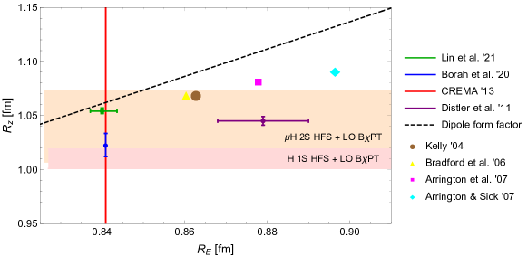
Figure 7: Correlation between the Zemach and charge radius of the proton. Our extractions based on LO B$\chi$PT are compared to results from Lin et al. [68], Borah et al. [69], CREMA [5], Distler et al. [70], Kelly [71], Bradford et al. [72], Arrington et al. [73], and Arrington & Sick [74].

Table 1: Determinations of the proton Zemach radius $R_{\mathrm{Z}}$, in units of fm.

$ep$ scattering		$\mu$H $2S$ hfs		H $1S$ hfs
Lin et al. ’21 [68]	Borah et al. ’20 [69]	Antognini et al. ’13 [5]	LO B$\chi$PT	Volotka et al. ’04  [75]	LO B$\chi$PT
$1.054^{+0.003}_{-0.002}$	$1.0227(107)$	$1.082(37)$	$1.040(33)$	$1.045(16)$	$1.010(9)$

VI Theory prediction for the ground-state hyperfine splitting in $\mu$H

The upcoming measurements of the $1S$ hfs in $\mu$H [8, 9, 10, 11] crucially rely on a precise theory prediction. The limiting uncertainty is given by the TPE, which is conventionally split into Zemach radius, polarizability and recoil contributions [13]:

$$E_{\text{hfs}}(1S,\mu\text{H})=\Big{[}183.797(7)\underbrace{-1.30653(17)\left(\frac{R_{\mathrm{Z}}}{\text{fm}}\right)+E_{\mathrm{F}}\,\Big{(}1.01656(4)\,\Delta_{\mathrm{recoil}}+1.00402\,\Delta_{\mathrm{pol.}}\Big{)}}_{\text{TPE including radiative corrections}}\Big{]}\,\text{meV},$$ (38)

see Appendix C and Table 2 for an itemized list of the individual contributions. As explained in Sec. IV.4, it is customary to refine the theory prediction of $1S$ hfs in $\mu$H with the help of the high-precision measurement of the $1S$ hfs in H. We do so by combining our B$\chi$PT prediction for the polarizability effect in the $\mu$H hfs, Eq. (17b), and the Zemach radius extracted from H spectroscopy, Eq. (37a), based on the same prediction for the polarizability effect in the H hfs. We arrive at:

$$E_{\text{hfs}}(1S,\mu\text{H}) = 182.640(18)\,\mathrm{meV},$$ (39a)

$$E^{\text{TPE}}_{\mathrm{hfs}}(1S,\mu\text{H}) = -1.157(16)\,\mathrm{meV},$$ (39b)

where $E^{\text{TPE}}_{\mathrm{hfs}}$ corresponds to the TPE including radiative corrections and recoil corrections from Ref. [33], as indicated by the curly brace in Eq. (38).

In Figs. 8 and 9, we compare our predictions to results from data-driven dispersive evaluations [14, 16] and HB EFT [58]. While almost all available predictions for the total hfs in $\mu$H are in agreement after the H refinement procedure, further improvements of the theory are required in order to compete with the anticipated experimental accuracy.

VII Conclusions and outlook

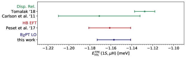
Figure 8: Two-photon-exchange effect on the $1S$ hyperfine splitting in $\mu$H [14, 58, 16].

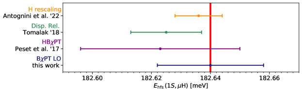
Figure 9: Predictions for the $1S$ hyperfine splitting in $\mu$H [13, 58, 16], compared to the projected uncertainty of the planned CREMA measurement (red vertical line).

We have presented the LO B$\chi$PT prediction for the $\mathcal{O}(\alpha^{5})$ polarizability effect on the hfs in H and $\mu$H, see Eq. (15). Contrary to the data-driven evaluations, the B$\chi$PT prediction is compatible with zero. This was expected from the HB$\chi$PT limit of the VVCS amplitudes, in particular $\bar{S}_{1}(0,Q^{2})$, which partially display a cancellation of the leading order in the chiral expansion of small $m_{\pi}$, see discussion in Sec. III.1. The small polarizability effect is then mainly a remnant of higher orders in the HB expansion.

A new formalism where the polarizability effect is split into contributions from the longitudinal-transverse and helicity-difference cross sections, $\sigma_{LT}$ and $\sigma_{TT}$, instead of contributions from the spin structure functions, $g_{1}$ and $g_{2}$, has been introduced in Eq. (12). It was shown that these contributions, $\Delta_{LT}$ and $\Delta_{TT}$, cancel by one order of magnitude when combined into $\Delta_{\mathrm{pol.}}$. Only $\Delta_{LT}$ and $\Delta_{TT}$ are good observables in the B$\chi$PT framework, for which the contributions from beyond the scale at which this EFT is safely applicable, $Q_{\mathrm{max}}>m_{\rho}=775$ MeV, are within the expected uncertainty. In addition, only $\Delta_{LT}$ and $\Delta_{TT}$ satisfy the conventionally assumed scaling with the reduced mass $m_{r}$ of the hydrogen-like system to $10\%$ relative accuracy, while the cancellations in $\Delta_{\mathrm{pol.}}$ enhance any violation in the scaling by one order of magnitude.

As shown in Fig. 4, our model-independent LO B$\chi$PT prediction is substantially smaller than the data-driven dispersive evaluations. An estimate for the effect of the $\Delta(1232)$-resonance [61], obtained from large-$N_{c}$ relations for the nucleon-to-delta transition form factors, shows that the discrepancy is likely to increase at the NLO. The smaller polarizability effect, in turn, leads to a smaller Zemach radius as extracted from the experimental $1S$ hfs in H and the $2S$ hfs in $\mu$H, cf. Eq. (37). Therefore, resolving the present discrepancy for the polarizability effect is crucial for the analysis of the forthcoming measurements of the $1S$ hfs in $\mu$H and the extraction of the Zemach radius.

The data-driven approach relies on empirical information on the inelastic spin structure functions, or the measured cross sections to be precise, as well as the elastic form factors and polarizabilities at $Q^{2}=0$. Due to the large cancellations between $\sigma_{LT}$ and $\sigma_{TT}$, as well as $g_{1}$ and $F_{2}$, precise parametrizations of the former are needed, and the uncertainty of the TPE evaluation has to be estimated with great care, taking into account all correlations. Furthermore, due to a lack of data at low-$Q$, one uses an interpolation from $Q^{2}=0$ to the onset of data [14]. As we showed in Sec. IV.3 based on LO B$\chi$PT, the quality of these approximations is rather poor and is yet another source of uncertainty. New data from the Jefferson Lab “Spin Physics Program” [17, 18, 19, 20, 21], including also the substantially extended dataset for $g_{2}$ [23], will allow for a re-evaluation of the polarizability effect on the hfs in H and $\mu$H.

An accurate theoretical prediction of the $1S$ hfs in $\mu$H is crucial for the future measurement campaigns, since it allows to reduce the search range for the resonance in experiment. Thus, one might find the resonance faster and acquire more statistics during the allocated beam time, see discussion in Ref. [13]. The present discrepancy between predictions for the polarizability effect can be mended if the high-precision measurement of the $1S$ hfs in H is implemented as a constraint. Applying this procedure, good agreement is found between all theory predictions for the total $1S$ hfs in $\mu$H hfs, see Fig. 9. Eventually, after a successful measurement of the $1S$ hfs in $\mu$H, one can combine it with the $1S$ hfs in H to disentangle the Zemach radius and polarizability effects, leveraging radiative corrections as explained in Ref. [13]. The empirical polarizability effect, obtained in this way, can reach a precision of $\sim 40$ ppm [13]. That is sufficient to discriminate between the presently inconsistent theoretical predictions.

Appendix A Two-photon-exchange master formula and dispersive approach

The proton-structure effects at $\mathcal{O}(\alpha^{5})$ are described by TPE in forward kinematics, i.e., by the diagram in Fig. 1 where the momentum transfer between the initial and final particles is vanishing. The (forward) TPE can be related to the amplitudes of (forward) VVCS off the proton, which in turn can be expressed in terms of proton structure functions via dispersion relations. A detailed review of the VVCS theory can be found in Ref. [36, Section 5]. Even though the TPE formalism is well-known, see for instance Ref. [14, 7], we will present here its derivation for the hfs.

As implied above, it is customary to split the TPE into leptonic and hadronic tensors ($L^{\mu\nu}$ and $T^{\mu\nu}$):

$$\mathcal{M} = \frac{1}{2}\!\int\!\frac{\mathrm{d}^{4}q}{i(2\pi)^{4}}\frac{1}{q^{4}}\left[\bar{u}(\ell)L_{\mu\nu}(\ell,q)u(\ell)\right]\left[\bar{N}(p)T^{\mu\nu}(p,q)N(p)\right]\!,$$ (40)

where $u(\ell)$ and $N(p)$ are the lepton and proton Dirac spinors, with $\ell$, $p$ and $q$ being the lepton, proton and photon four-momenta (see Fig. 1), respectively. Here, a factor of $\nicefrac{{1}}{{2}}$ has been introduced to avoid double counting when contracting the crossing-invariant tensors.

Only the spin-dependent part of the forward VVCS will contribute to the hfs. For the proton, it reads:

$$T^{\mu\nu}_{A}(q,p) = -\frac{1}{M}\gamma^{\mu\nu\alpha}q_{\alpha}\,S_{1}(\nu,Q^{2})+\frac{Q^{2}}{M^{2}}\gamma^{\mu\nu}S_{2}(\nu,Q^{2}),$$ (41)

where $S_{1}$ and $S_{2}$ are two independent scalar functions of the photon lab-frame energy $\nu$ and the photon virtuality $Q^{2}=-q^{2}=\mathbf{q}^{2}-\nu^{2}$. Equivalently, one can write Eq. (41) with the help of the spin four-vector $\mathtt{s}^{\alpha}$ (satisfying $\mathtt{s}^{2}=-1$ and $\mathtt{s}\cdot p=0$):

$$T^{\mu\nu}_{A}(q,p) = \frac{i}{M}\,\epsilon^{\mu\nu\alpha\beta}\,q_{\alpha}\mathtt{s}_{\beta}\,S_{1}(\nu,Q^{2})+\frac{i}{M^{3}}\,\epsilon^{\mu\nu\alpha\beta}\,q_{\alpha}(p\cdot q\ \mathtt{s}_{\beta}-\mathtt{s}\cdot q\ p_{\beta})\,S_{2}(\nu,Q^{2}).$$ (43)

Since $T_{A}^{\mu\nu}$ is antisymmetric in its indices, it is sufficient to replace the lepton tensor with the antisymmetric part of the tree-level QED amplitude of forward VVCS [in the structureless limit with the Dirac and Pauli form factors $F_{1}\rightarrow 1$ and $F_{2}\rightarrow 0$, cf. Eqs. (41) and (51)]:

$$L_{A}^{\mu\nu}=\frac{-2\pi\alpha\,Q^{2}}{(\ell\cdot q)^{2}-\mbox{$\frac{1}{4}$}Q^{4}}\,\gamma^{\mu\nu\alpha}q_{\alpha}.$$ (45)

The lepton and proton momenta are of typical atomic scales, thus, much smaller than the other scales we are considering. Therefore, in the center-of-mass frame, we assume both of them to be at rest, $p=\nicefrac{{M}}{{m}}\,\ell=(M,\boldsymbol{0})$:

$$\left[\bar{u}(\ell)\gamma_{\mu\nu\alpha}q^{\alpha}\,u(\ell)\right]\left[\bar{N}(p)\gamma^{\mu\nu}\,N(p)\right]=8\nu\,\boldsymbol{s}\cdot\boldsymbol{S},\qquad$$ (46)

$$\left[\bar{u}(\ell)\gamma_{\mu\nu\alpha}q^{\alpha}u(\ell)\right]\left[\bar{N}(p)\gamma^{\mu\nu\beta}q_{\beta}N(p)\right]=\frac{8}{3}(\nu^{2}-2Q^{2})\,\boldsymbol{s}\cdot\boldsymbol{S},$$

with the lepton and proton spin operators $\boldsymbol{s}$ and $\boldsymbol{S}$, and $\ell\cdot q=m\nu$.

The forward TPE generates a $\delta(\vec{r}\,)$-function potential: $V(r)=\mathcal{M}\,\delta(\vec{r}\,)$. Treated in perturbation theory, such kind of potential generates an energy shift of the $nS$ levels: $E_{nS}=\phi_{n}^{2}\,\mathcal{M}$, where $\phi_{n}^{2}=1/(\pi a^{3}n^{3})$ is the hydrogen wave function at the origin. When acting on the wave functions, the product of spin operators can be replaced by the atom’s total angular momentum $f$ [76]:

$$\boldsymbol{s}\cdot\boldsymbol{S}\xrightarrow{{nS\text{ level }}}\mbox{$\frac{1}{2}$}\left[f(f+1)-\mbox{$\frac{3}{2}$}\right].$$ (47)

Recalling that the $nS$ hfs is defined as the splitting between $S$ levels with $f=1$ and $f=0$, we finally arrive at the following master formula for the TPE contribution to the hfs in terms of proton VVCS amplitudes:

$$E^{\mathrm{TPE}}_{\mathrm{hfs}}(nS) = \frac{E_{\mathrm{F}}}{n^{3}}\frac{4m}{1+\kappa}\frac{1}{i}\int_{-\infty}^{\infty}\!\frac{\mathrm{d}\nu}{2\pi}\int\!\!\frac{\mathrm{d}\mathbf{q}}{(2\pi)^{3}}\,\frac{1}{Q^{4}-4m^{2}\nu^{2}}\left\{\frac{\left(2Q^{2}-\nu^{2}\right)}{Q^{2}}S_{1}(\nu,Q^{2})+\frac{3\nu}{M}S_{2}(\nu,Q^{2})\right\}.$$ (48)

The Lamb shift analogue reads

$$E^{\mathrm{TPE}}_{nS}=8\pi\alpha m\,\phi_{n}^{2}\,\frac{1}{i}\int_{-\infty}^{\infty}\!\frac{\mathrm{d}\nu}{2\pi}\int\!\!\frac{\mathrm{d}\mathbf{q}}{(2\pi)^{3}}\frac{\left(Q^{2}-2\nu^{2}\right)T_{1}(\nu,Q^{2})-(Q^{2}+\nu^{2})\,T_{2}(\nu,Q^{2})}{Q^{4}(Q^{4}-4m^{2}\nu^{2})},$$ (49)

where $T_{1}$ and $T_{2}$ are the spin-independent forward VVCS amplitudes. The VVCS amplitudes can be split into Born and non-Born parts:

$$S_{1}(\nu,Q^{2}) = S_{1}^{\mathrm{Born}}(\nu,Q^{2})+\bar{S}_{1}(\nu,Q^{2}),$$ (50a)

$$S_{2}(\nu,Q^{2}) = S_{2}^{\mathrm{Born}}(\nu,Q^{2})+\bar{S}_{2}(\nu,Q^{2}),$$ (50b)

where Born corresponds to the simplest tree-level diagrams with a proton in the intermediate state, and non-Born corresponds to everything else. The finite-size recoil and Zemach radius effects are described by the well-known Born part of the VVCS amplitudes [77]:

$$S_{1}^{\mathrm{Born}}(\nu,Q^{2}) = \frac{2\pi\alpha}{M}\bigg{[}\frac{4M^{2}Q^{2}\,G_{M}(Q^{2})F_{1}(Q^{2})}{Q^{4}-4M^{2}\nu^{2}}-F_{2}^{2}(Q^{2})\bigg{]},$$ (51a)

$$S_{2}^{\mathrm{Born}}(\nu,Q^{2}) = -\,\frac{8\pi\alpha M^{2}\nu}{Q^{4}-4M^{2}\nu^{2}}\,G_{M}(Q^{2})F_{2}(Q^{2}),$$ (51b)

where $F_{1}(Q^{2})$ and $F_{2}(Q^{2})$ are the Dirac and Pauli form factors of the proton, and $G_{M}(Q^{2})=F_{1}(Q^{2})+F_{2}(Q^{2})$ is the magnetic Sachs form factor. The Zemach radius and its effect on the hfs are defined in Eqs. (6) and (7). Exact formulas for the TPE recoil contribution can be found for instance in Ref. [7]. The polarizability effect is described by the non-Born part of the VVCS amplitudes.

Using the general principles of analyticity, unitarity, crossing symmetry and gauge invariance, one can conveniently express the spin-dependent VVCS amplitudes through the proton spin structure functions $g_{1}(x,Q^{2})$ and $g_{2}(x,Q^{2})$ by means of the optical theorem:

$$\operatorname{Im}S_{1}(\nu,Q^{2}) = \frac{4\pi^{2}\alpha}{\nu}\,g_{1}(x,Q^{2})=\frac{M\nu^{2}}{\nu^{2}+Q^{2}}\left[\frac{Q}{\nu}\sigma_{LT}+\sigma_{TT}\right](\nu,Q^{2}),$$ (52a)

$$\operatorname{Im}S_{2}(\nu,Q^{2}) = \frac{4\pi^{2}\alpha M}{\nu^{2}}\,g_{2}(x,Q^{2})=\frac{M^{2}\nu}{\nu^{2}+Q^{2}}\left[\frac{\nu}{Q}\sigma_{LT}-\sigma_{TT}\right](\nu,Q^{2}),\qquad\quad$$ (52b)

and dispersion relations:

$$\bar{S}_{1}(\nu,Q^{2}) = \frac{2\pi\alpha}{M}\Bigg{\{}\left[F_{2}^{2}(Q^{2})+4I_{1}(Q^{2})\right]+\frac{32M^{4}\nu^{2}}{Q^{6}}\int_{0}^{x_{0}}\!\mathrm{d}x\,\frac{x^{2}g_{1}(x,Q^{2})}{1-x^{2}(\nu/\nu_{\mathrm{el}})^{2}-i0^{+}}\Bigg{\}},$$ (53a)

$$\nu\bar{S}_{2}(\nu,Q^{2}) = \frac{64\pi\alpha M^{4}\nu^{2}}{Q^{6}}\int_{0}^{x_{0}}\!\mathrm{d}x\,\frac{x^{2}g_{2}(x,Q^{2})}{1-x^{2}(\nu/\nu_{\mathrm{el}})^{2}-i0^{+}},$$ (53b)

with $\nu_{\mathrm{el}}=\nicefrac{{Q^{2}}}{{2M}}$ and $I_{1}(Q^{2})$ defined in Eq. (11). As shown in Eq. (52), the spin structure functions correspond to certain combinations of photoabsorption cross sections. Here, $\sigma_{LT}$ is the longitudinal-transverse photoabsorption cross section describing a spin-flip of the proton, and $\sigma_{TT}=\nicefrac{{1}}{{2}}\,(\sigma_{1/2}-\sigma_{3/2})$ is the helicity-difference cross section for transversely polarized photons, where the subscripts on $\sigma_{1/2}$ and $\sigma_{3/2}$ denote the total helicity of the $\gamma^{\ast}N$ state.

To solve Eq. (48) one uses a Wick rotation to imaginary energies, and hyperspherical coordinates. Employing the dispersive representation from Eq. (53), after the angular integrations one obtains the polarizability effect as presented in Eq. (10), where one conventionally splits into contributions from $g_{1}$ and $g_{2}$. As we explain in our paper, in view of the uncertainty estimate, it is favorable to consider instead a splitting into contributions from $\sigma_{LT}$ and $\sigma_{TT}$, derived by us in Eq. (12).

It is worth to discuss some subtleties entering the definition of the polarizability effect through the non-Born VVCS amplitudes in the dispersive approach. Naively, one would expect the Born and non-Born amplitudes to be expressed entirely through elastic form factors and inelastic structure functions, respectively. Instead, one finds:

$$S_{1}^{\mathrm{elastic}}(\nu,Q^{2})-S_{1}^{\mathrm{Born}}(\nu,Q^{2}) = \bar{S}_{1}(\nu,Q^{2})-S_{1}^{\mathrm{inelastic}}(\nu,Q^{2})=\frac{2\pi\alpha}{M}F_{2}^{2}(Q^{2}),$$ (54a)

$$\left[\nu S_{2}\right]^{\mathrm{elastic}}(\nu,Q^{2})-\nu S_{2}^{\mathrm{Born}}(\nu,Q^{2}) = \nu\bar{S}_{2}(\nu,Q^{2})-\left[\nu S_{2}\right]^{\mathrm{inelastic}}(\nu,Q^{2})=-2\pi\alpha\,F_{2}(Q^{2})G_{M}(Q^{2}),$$ (54b)

where $S_{1}^{\mathrm{elastic}}$ and $\left[\nu S_{2}\right]^{\mathrm{elastic}}$ are pure nucleon-pole terms. In Eq. (53a), the necessary conversion term to obtain the non-Born amplitude, given on the right-hand side of Eq. (54a), is easily seen. Here, even though $S_{1}$ satisfies an unsubtracted dispersion relation, we wrote a once-subtracted dispersion relation, with the subtraction term $\bar{S}_{1}(0,Q^{2})$ defined in Eq. (27). This is useful to emphasize the interplay of the elastic Pauli form factor $F_{2}$ and the inelastic spin structure function $g_{1}$, as explained in Sections II and IV.3. For Eq. (53b), the applied conversion procedure is less obvious. Starting from a dispersion relation for $\nu S_{2}$:

$$\nu S_{2}(\nu,Q^{2})=2\pi\alpha\,\frac{2}{\tau}\int_{0}^{1}\!\mathrm{d}x\,\frac{g_{2}(x,Q^{2})}{1-x^{2}(\nu/\nu_{\mathrm{el}})^{2}-i0^{+}},$$ (55)

we separate the inelastic part (i.e., limit the integration to $x\in\{0,x_{0}\}$) and add the conversion term from the right-hand side of Eq. (54b). The latter then cancels the inelastic part of the zeroth moment of the $g_{2}$ structure function, due to the Burkhardt-Cottingham (BC) sum rule [78]:

$$0=\int_{0}^{1}\mathrm{d}x\,g_{2}(x,\,Q^{2})=\int_{0}^{x_{0}}\mathrm{d}x\,g_{2}(x,\,Q^{2})-\frac{\tau}{2}F_{2}(Q^{2})G_{M}(Q^{2}),$$ (56)

leading to Eq. (53b). Thus, splitting into Born and non-Born amplitudes, the BC sum rule constraint is automatically satisfied. In other words, we showed that:

$$\nu S_{2}^{\mathrm{Born}}(\nu,Q^{2})\big{|}_{\nu\rightarrow 0}=\nu\bar{S}_{2}(\nu,Q^{2})\big{|}_{\nu\rightarrow 0}=0.$$ (57)

Appendix B Electron vacuum polarization correction

Figure 10: Two-photon exchange with vacuum-polarization insertion at $O(\alpha^{6})$.

In this appendix, we consider the one-loop eVP correction to the TPE, shown in Fig. 10. This amounts to multiplying the integrand in Eq. (48) with $\left[1-\overline{\Pi}^{(1)}(Q^{2})\right]^{-2}$, where the VP is given by:

$$\overline{\Pi}^{(1)}(Q^{2})=\Pi^{(1)}(Q^{2})-\Pi^{(1)}(0) =\frac{\alpha}{3\pi}\left[2\left(1-\frac{1}{2\tau_{e}}\right)\left(\sqrt{1+\frac{1}{\tau_{e}}}\operatorname{arccoth}\sqrt{1+\frac{1}{\tau_{e}}}-1\right)+\frac{1}{3}\right],$$ (58)

with $\tau_{e}=Q^{2}/4m_{e}^{2}$ and $m_{e}$ the electron mass. The resulting corrections to the polarizability effect are given in Eq. (17).

Table 2: $1S$ hfs in $\mu$H. All values in meV

	Contribution	Our Choice	Reference
h1	Fermi energy, $(Z\alpha)^{4}$	$182.44333$
h2	Breit corr., $(Z\alpha)^{6}$	$0.01457$
h4	$\mu$ anomalous magnetic moment corr., $\alpha(Z\alpha)^{4}$	$0.21271$
h5	eVP in 2nd-order PT, $\alpha^{2}(Z\alpha)^{4}m_{r}$	$0.73449$	[79, Table 1 b)]
h7	Two-loop corr. to Fermi energy, $\alpha^{2}(Z\alpha)^{4}m_{r}$	$0.00556$	[79, Table 2 c) and d)]
h8	One-loop eVP in $1\gamma$ int., $\alpha(Z\alpha)^{4}m_{r}$	$0.37465$	[79, Table 1 a)]
h9	Two-loop eVP in $1\gamma$ int., $\alpha^{2}(Z\alpha)^{4}m_{r}$	$0.00292$	[79, Table 2 a) and b)]
h10	Further two-loop eVP corr. in 2nd and 3rd-order PT	$0.00387$	[79, Table 2 e), f) and g)]
h11	$\mu$VP	$0.00729$	$\sim E_{\mathrm{F}}\,\alpha(Z\alpha)\,3/4$
h13	Vertex, $\alpha(Z\alpha)^{5}$	$-0.02484$	$\sim E_{\mathrm{F}}\,\alpha(Z\alpha)\left[\ln 2-13/4\right]$
h14	Higher-order corr.  $\alpha(Z\alpha)^{6}$	$-0.00128$	[80, Eq. 7.1]
h18	hVP, $\alpha^{6}$	$0.00356$	[81]
h19	Weak interaction contribution	$0.00221$	[82, Eq. 374]
h28	Recoil corr. with $p$ AMM, $\alpha^{6}$	$0.01752$	[14, Eq. 22] and [83]

Table 3: $2S$ hfs in $\mu$H. All values in meV

	Contribution	Our Choice	Reference
h1	Fermi energy, $(Z\alpha)^{4}$	$22.80542$
h2	Breit corr., $(Z\alpha)^{6}$	$0.00258$
h4	$\mu$ anomalous magnetic moment corr., $\alpha(Z\alpha)^{4}$	$0.02659$
h5	eVP in 2nd-order PT, $\alpha^{2}(Z\alpha)^{4}m_{r}$	$0.07447$	[79, Table 1 b)]
h7	Two-loop corr. to Fermi energy, $\alpha^{2}(Z\alpha)^{4}m_{r}$	$0.00056$	[79, Table 2 c) and d)]
h8	One-loop eVP in $1\gamma$ int., $\alpha(Z\alpha)^{4}m_{r}$	$0.04828$	[79, Table 1 a)]
h9	Two-loop eVP in $1\gamma$ int., $\alpha^{2}(Z\alpha)^{4}m_{r}$	$0.00037$	[79, Table 2 a) and b)]
h10	Further two-loop eVP corr. in 2nd & 3rd-order PT	$0.00037$	[79, Table 2 e), f) and g)]
h11	$\mu$VP	$0.00091$	$\sim E_{\mathrm{F}}\,\alpha(Z\alpha)\,3/4$
h13	Vertex, $\alpha(Z\alpha)^{5}$	$-0.00311$	$\sim E_{\mathrm{F}}\,\alpha(Z\alpha)\left[\ln 2-13/4\right]$
h14	Higher-order corr.  $\alpha(Z\alpha)^{6}$	$-0.00013$	[80, Eq. 7.1]
h18	hVP, $\alpha^{6}$	$0.0006(1)$	[84]
h19	Weak interaction contribution	$0.00028$	[82, Eq. 374]
h21	Higher-order finite-size corr. to Fermi energy	$-0.0022\,r_{p}^{2}+0.0009$	[85, Eq. 107]
		$\approx-0.00065$
h28	Recoil corr. with $p$ AMM, $\alpha^{6}$	$0.00185$	[58, Eqs. 1.3 and 2.13]

Appendix C Theory compilation for hyperfine splitting in $\mu$H

In this appendix, we present the details of our theory compilations for the $1S$ and $2S$ hfs in $\mu$H, shown in Eqs. (35) and (38). All individual contributions, except the TPE, are listed in Tables 2 and 3. The notation is the same as in Ref. [6]. The difference with Ref. [86] is in the inclusion of ##h10, h14, h18, h19 and h21, as well as some additional radiative corrections to the TPE evaluated in Ref. [13]. Compared to Refs. [6, 84], we suggest to use Eq. (7.1) from Ref. [80]:

$$E^{[\alpha(Z\alpha)^{6}]}_{nS\text{-hfs}} = \frac{\alpha(Z\alpha)^{2}}{\pi}\,\frac{E_{\mathrm{F}}}{n^{3}}\left\{-\frac{8}{3}\ln^{2}\frac{2n}{Z\alpha}+\left[\frac{37}{36}+\frac{8}{15}+7(n-1)\right]\ln\frac{n}{2Z\alpha}\right.$$

$$\left.+\left[\frac{22}{3}\ln 2-\frac{2\pi^{2}}{9}+18-\frac{457}{2700}-\left(4+\frac{2993}{8640}\right)(n-1)\right]\right\},$$

for the higher-order corrections of $\mathcal{O}(\alpha(Z\alpha)^{6})$ [#h14]. This includes higher-order muon vacuum polarization corrections. Previously included were only the logarithmically enhanced terms [84]. The effect on the TPE from eVP corrections to the wave function is given in Ref. [87, Eq. (B3)]. For the radius-independent term, we are keeping the error estimate from Ref. [58], which does take into account missing higher-order recoil corrections.

Appendix D Expansions in terms of polarizabilities

In the following, we will present two further low-energy expansions of the polarizability effect in the hfs. Due to the high-energy asymptotics of the TPE contribution to the hfs, these formulas will merely serve illustrative purposes, while their approximation of the full result is rather poor. Up to and including second moments of the structure functions, Eq. (10) can be written as [62]:

$$\delta_{1} = 2\int_{0}^{\infty}\frac{\mathrm{d}Q}{Q}\frac{1}{(v_{l}+1)^{2}}\bigg{\{}4(5+4v_{l})\,\bar{I}_{1}(Q^{2})-\frac{11+9v_{l}}{(v_{l}+1)}\left[\frac{M^{2}Q^{2}}{2\alpha}\,\gamma_{0}(Q^{2})+\frac{32Z^{2}M^{6}}{Q^{6}}\int_{0}^{x_{0}}\mathrm{d}x\,x^{4}\,g_{2}(x,Q^{2})\right]\!\bigg{\}},\qquad\quad$$ (59a)

$$\delta_{2} = -24\int_{0}^{\infty}\frac{\mathrm{d}Q}{Q}\frac{1}{(v_{l}+1)^{2}}\left\{\frac{M^{2}Q^{2}}{2\alpha}\,\left[\delta_{LT}(Q^{2})-\gamma_{0}(Q^{2})\right]-\frac{32Z^{2}M^{6}}{Q^{6}}\int_{0}^{x_{0}}\mathrm{d}x\,x^{4}\,g_{2}(x,Q^{2})\right\},$$ (59b)

where $\gamma_{0}(Q^{2})$ and $\delta_{LT}(Q^{2})$ are the forward spin and longitudinal-transverse polarizabilities of the proton,

$$\gamma_{0}(Q^{2}) = \frac{16\alpha M^{2}}{Q^{6}}\int_{0}^{x_{0}}\mathrm{d}x\,x^{2}\Big{[}g_{1}-x^{2}\tau^{-1}g_{2}\Big{]}(x,Q^{2})=\frac{1}{2\pi^{2}}\int_{\nu_{0}}^{\infty}\frac{\mathrm{d}\nu}{\nu^{3}}\,\sigma_{TT}(\nu,Q^{2}),$$ (60a)

$$\delta_{LT}(Q^{2}) = \frac{16Z^{2}\alpha M^{2}}{Q^{6}}\int_{0}^{x_{0}}\mathrm{d}x\,x^{2}\big{[}g_{1}+g_{2}\big{]}(x,Q^{2})=\frac{1}{2\pi^{2}}\int_{\nu_{0}}^{\infty}\frac{\mathrm{d}\nu}{Q\nu^{2}}\,\sigma_{LT}(\nu,Q^{2}).$$ (60b)

The first term in this expansion, corresponds to the $\bar{S}_{1}(0,Q^{2})$ subtraction term already discussed in Sec. IV.3.

Analogously to Ref. [27, Eq. (12)], we try to find an approximation for the hfs master formula assuming that the photon energy in the atomic system is small compared to all other scales. Thus, we expand the numerator of Eq. (48) around $\nu=0$. The resulting approximate formula for the polarizability contribution to the hfs we call $\tilde{E}$:

$$\tilde{E}(nS)=\frac{E_{\mathrm{F}}}{n^{3}}\frac{4\alpha}{\pi mM}\frac{1}{1+\kappa}\int_{0}^{\infty}\!\mathrm{d}Q\,Q\,(v_{l}-1)\,\bar{I}_{1}(Q^{2}).$$ (61)

For B$\chi$PT, it gives:

$$\tilde{E}(1S,\mathrm{H}) = 3.0\,\text{peV},$$ (62a)

$$\tilde{E}(1S,\mu\mathrm{H}) = 19.0\,\upmu\text{eV}.$$ (62b)

In Fig. 11, we show Eq. (61) as a running integral with cut-off $Q_{\mathrm{max}}$ (gray line), this time for the $2S$ hfs in $\mu$H. In addition, we show the contributions of the longitudinal-transverse (orange line) and helicity-difference (blue line) cross sections to Eq. (61), and the exact result from Eq. (10). One can easily see that the quality of the approximation is indeed rather poor.

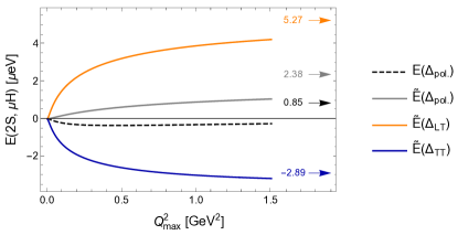
Figure 11: Polarizability effect on the $2S$ hyperfine splitting in $\mu$H: Comparison of exact result (10) [black dashed line] and approximate formula (61) [gray solid line].

References

- Pohl et al. [2010] Randolf Pohl et al., “The size of the proton,” Nature 466, 213–216 (2010).
- Pohl et al. [2016a] Randolf Pohl et al. (CREMA), “Laser spectroscopy of muonic deuterium,” Science 353, 669–673 (2016a).
- Krauth et al. [2021] Julian J. Krauth et al., “Measuring the -particle charge radius with muonic helium-4 ions,” Nature 589, 527–531 (2021).
- Antognini et al. [2022a] Aldo Antognini et al., “Muonic-Atom Spectroscopy and Impact on Nuclear Structure and Precision QED Theory,” (2022a), arXiv:2210.16929 [nucl-th] .
- Antognini et al. [2013a] Aldo Antognini, Francois Nez, Karsten Schuhmann, Fernando D. Amaro, et al., “Proton Structure from the Measurement of Transition Frequencies of Muonic Hydrogen,” Science 339, 417–420 (2013a).
- Antognini et al. [2013b] Aldo Antognini, Franz Kottmann, Francois Biraben, Paul Indelicato, et al., “Theory of the Lamb shift and hyperfine splitting in muonic hydrogen,” Annals Phys. 331, 127–145 (2013b), arXiv:1208.2637 [physics.atom-ph] .
- Carlson et al. [2011] Carl E. Carlson, Vahagn Nazaryan, and Keith Griffioen, “Proton structure corrections to hyperfine splitting in muonic hydrogen,” Phys. Rev. A 83, 042509 (2011), arXiv:1101.3239 [physics.atom-ph] .
- Amaro et al. [2022] P. Amaro et al., “Laser excitation of the -hyperfine transition in muonic hydrogen,” SciPost Phys. 13, 020 (2022), arXiv:2112.00138 [physics.atom-ph] .
- Pizzolotto et al. [2021] C. Pizzolotto et al., “Measurement of the muon transfer rate from muonic hydrogen to oxygen in the range 70-336 K,” Phys. Lett. A 403, 127401 (2021), arXiv:2105.06701 [physics.atom-ph] .
- Pizzolotto et al. [2020] C. Pizzolotto et al., “The FAMU experiment: muonic hydrogen high precision spectroscopy studies,” Eur. Phys. J. A 56, 185 (2020).
- Sato et al. [2014] Masaharu Sato et al., “Laser spectroscopy of the hyperfine splitting energy in the ground state of muonic hydrogen,” in Proceedings, 20th International Conference on Particles and Nuclei (PANIC 14), Hamburg, Germany, August 24-29, 2014 (2014).
- Pohl et al. [2016b] Randolf Pohl et al., “Laser Spectroscopy of Muonic Atoms and Ions,” in Proceedings, 12th International Conference on Low Energy Antiproton Physics (LEAP2016), Kanazawa, Japan, March 6-11, 2016 (2016) arXiv:1609.03440 [physics.atom-ph] .
- Antognini et al. [2022b] Aldo Antognini, Franziska Hagelstein, and Vladimir Pascalutsa, “The proton structure in and out of muonic hydrogen,” Ann. Rev. Nucl. Part. Sci. 72, 389–418 (2022b), arXiv:2205.10076 [nucl-th] .
- Carlson et al. [2008] Carl E. Carlson, Vahagn Nazaryan, and Keith Griffioen, “Proton structure corrections to electronic and muonic hydrogen hyperfine splitting,” Phys. Rev. A 78, 022517 (2008), arXiv:0805.2603 [physics.atom-ph] .
- Faustov et al. [2006] R.N. Faustov, I.V. Gorbacheva, and A.P. Martynenko, “Proton polarizability effect in the hyperfine splitting of the hydrogen atom,” Proc. SPIE Int. Soc. Opt. Eng. 6165, 0M (2006), arXiv:hep-ph/0610332 [hep-ph] .
- Tomalak [2019] Oleksandr Tomalak, “Two-Photon Exchange Correction to the Lamb Shift and Hyperfine Splitting of S Levels,” Eur. Phys. J. A 55, 64 (2019), arXiv:1808.09204 [hep-ph] .
- Chen [2008] J. P. Chen, “Highlights and Perspectives of the JLab Spin Physics Program,” Advanced Studies Institute on Symmetries and Spin (SPIN-Praha-2007) Prague, Czech Republic, July 8-14, 2007, Eur. Phys. J. ST 162, 103–116 (2008), arXiv:0804.4486 [nucl-ex] .
- Adhikari et al. [2018] K. P. Adhikari et al. (CLAS), “Measurement of the Dependence of the Deuteron Spin Structure Function and its Moments at Low with CLAS,” Phys. Rev. Lett. 120, 062501 (2018), arXiv:1711.01974 [nucl-ex] .
- Zheng et al. [2021] X. Zheng et al. (CLAS), “Measurement of the proton spin structure at long distances,” Nature Phys. 17, 736–741 (2021), arXiv:2102.02658 [nucl-ex] .
- Sulkosky et al. [2020] V. Sulkosky et al. (Jefferson Lab E97-110), “Measurement of the 3He spin-structure functions and of neutron (3He) spin-dependent sum rules at ,” Phys. Lett. B 805, 135428 (2020), arXiv:1908.05709 [nucl-ex] .
- Sulkosky et al. [2021] Vincent Sulkosky et al. (E97-110), “Puzzle with the precession of the neutron spin,” Nature Phys. 17, 687–692 (2021), [Erratum: Nature Phys. 18, (2022)], arXiv:2103.03333 [nucl-ex] .
- Zielinski [2017 [nucl-ex/1708.08297]] Ryan Zielinski, The g2p Experiment: A Measurement of the Proton’s Spin Structure Functions, Ph.D. thesis, New Hampshire U. (2017 [nucl-ex/1708.08297]), arXiv:nucl-ex/1708.08297 [nucl-ex] .
- Ruth et al. [2022] D. Ruth et al. (Jefferson Lab Hall A g2p), “Proton spin structure and generalized polarizabilities in the strong quantum chromodynamics regime,” Nature Phys. 18, 1441–1446 (2022), arXiv:2204.10224 [nucl-ex] .
- Weinberg [1979] Steven Weinberg, “Phenomenological Lagrangians,” Physica A 96, 327 (1979).
- Gasser and Leutwyler [1984] J. Gasser and H. Leutwyler, “Chiral Perturbation Theory to One Loop,” Ann. Phys. 158, 142 (1984).
- Gasser et al. [1988] J. Gasser, M. E. Sainio, and A. Švarc, “Nucleons with Chiral Loops,” Nucl. Phys. B 307, 779 (1988).
- Alarcón et al. [2014] Jose Manuel Alarcón, Vadim Lensky, and Vladimir Pascalutsa, “Chiral perturbation theory of muonic hydrogen Lamb shift: polarizability contribution,” Eur. Phys. J. C 74, 2852 (2014), arXiv:1312.1219 [hep-ph] .
- Gegelia et al. [2003] J. Gegelia, G. Japaridze, and X. Q. Wang, “Is heavy baryon approach necessary?” J. Phys. G29, 2303–2309 (2003), arXiv:hep-ph/9910260 .
- Fuchs et al. [2003] T. Fuchs, J. Gegelia, G. Japaridze, and S. Scherer, “Renormalization of relativistic baryon chiral perturbation theory and power counting,” Phys. Rev. D 68, 056005 (2003), arXiv:hep-ph/0302117 .
- Pascalutsa et al. [2007] Vladimir Pascalutsa, Marc Vanderhaeghen, and Shin Nan Yang, “Electromagnetic excitation of the -resonance,” Phys. Rept. 437, 125–232 (2007), arXiv:hep-ph/0609004 .
- Geng [2013] Lisheng Geng, “Recent developments in SU(3) covariant baryon chiral perturbation theory,” Front. Phys. China 8, 328–348 (2013), arXiv:1301.6815 [nucl-th] .
- Pachucki [1996] Krzysztof Pachucki, “Theory of the Lamb shift in muonic hydrogen,” Phys. Rev. A 53, 2092–2100 (1996).
- Antognini et al. [2022c] Aldo Antognini, Yong-Hui Lin, and Ulf-G. Meißner, “Precision calculation of the recoil–finite-size correction for the hyperfine splitting in muonic and electronic hydrogen,” Phys. Lett. B 835, 137575 (2022c), arXiv:2208.04025 [nucl-th] .
- Hagelstein and Pascalutsa [2021] Franziska Hagelstein and Vladimir Pascalutsa, “The subtraction contribution to the muonic-hydrogen Lamb shift: A point for lattice QCD calculations of the polarizability effect,” Nucl. Phys. A 1016, 122323 (2021), arXiv:2010.11898 [hep-ph] .
- Biloshytskyi et al. [2024] Volodymyr Biloshytskyi, Iulian Ciobotaru-Hriscu, Franziska Hagelstein, Vadim Lensky, and Vladimir Pascalutsa, “QED of Bernabéu-Tarrach sum rule for electric polarizability and its implication for the Lamb shift,” Phys. Rev. D 109, 016026 (2024), arXiv:2305.08814 [hep-ph] .
- Hagelstein et al. [2016] Franziska Hagelstein, Rory Miskimen, and Vladimir Pascalutsa, “Nucleon Polarizabilities: from Compton Scattering to Hydrogen Atom,” Prog. Part. Nucl. Phys. 88, 29–97 (2016), arXiv:1512.03765 [nucl-th] .
- Nazaryan et al. [2006] Vahagn Nazaryan, Carl E. Carlson, and Keith A. Griffioen, “New experimental constraints on polarizability corrections to hydrogen hyperfine structure,” Phys. Rev. Lett. 96, 163001 (2006), arXiv:hep-ph/0512108 [hep-ph] .
- Lensky and Pascalutsa [2010] Vadim Lensky and Vladimir Pascalutsa, “Predictive powers of chiral perturbation theory in Compton scattering off protons,” Eur. Phys. J. C 65, 195–209 (2010), 0907.0451 [hep-ph] .
- Patrignani et al. [2016] C. Patrignani et al. (Particle Data Group), “Review of Particle Physics,” Chin. Phys. C 40, 100001 (2016).
- Lensky et al. [2014] Vadim Lensky, Jose Manuel Alarcón, and Vladimir Pascalutsa, “Moments of nucleon structure functions at next-to-leading order in baryon chiral perturbation theory,” Phys. Rev. C 90, 055202 (2014), arXiv:1407.2574 [hep-ph] .
- Alarcón et al. [2020a] Jose Manuel Alarcón, Franziska Hagelstein, Vadim Lensky, and Vladimir Pascalutsa, “Forward doubly-virtual Compton scattering off the nucleon in chiral perturbation theory: the subtraction function and moments of unpolarized structure functions,” Phys. Rev. D 102, 014006 (2020a), arXiv:2005.09518 [hep-ph] .
- Alarcón et al. [2020b] Jose Manuel Alarcón, Franziska Hagelstein, Vadim Lensky, and Vladimir Pascalutsa, “Forward doubly-virtual Compton scattering off the nucleon in chiral perturbation theory: II. Spin polarizabilities and moments of polarized structure functions,” Phys. Rev. D 102, 114026 (2020b), arXiv:2006.08626 [hep-ph] .
- Pascalutsa and Phillips [2003] Vladimir Pascalutsa and Daniel R. Phillips, “Effective theory of the in Compton scattering off the nucleon,” Phys. Rev. C 67, 055202 (2003), nucl-th/0212024 .
- Bernard et al. [2003] Veronique Bernard, Thomas R. Hemmert, and Ulf-G. Meissner, “Spin structure of the nucleon at low-energies,” Phys. Rev. D 67, 076008 (2003), arXiv:hep-ph/0212033 [hep-ph] .
- Bernard [2008] Véronique Bernard, “Chiral perturbation theory and baryon properties,” Progress in Particle and Nucl. Phys. 60, 82–160 (2008), 0706.0312 [hep-ph] .
- Bernard et al. [2013] Veronique Bernard, Evgeny Epelbaum, Hermann Krebs, and Ulf G. Meißner, “New insights into the spin structure of the nucleon,” Phys. Rev. D 87, 054032 (2013), arXiv:1209.2523 [hep-ph] .
- Hemmert et al. [1997a] Thomas R. Hemmert, Barry R. Holstein, and Joachim Kambor, “Systematic expansion for spin particles in baryon chiral perturbation theory,” Phys. Lett. B 395, 89–95 (1997a), arXiv:hep-ph/9606456 [hep-ph] .
- Ji and Osborne [2001] Xiang-Dong Ji and Jonathan Osborne, “Generalized sum rules for spin dependent structure functions of the nucleon,” J. Phys. G 27, 127 (2001), arXiv:hep-ph/9905410 [hep-ph] .
- Vijaya Kumar et al. [2000] K. B. Vijaya Kumar, J. A. McGovern, and M. C. Birse, “Spin polarisabilities of the nucleon at NLO in the chiral expansion,” Phys. Lett. B 479, 167–172 (2000), arXiv:hep-ph/0002133 .
- Hemmert et al. [1997b] Thomas R. Hemmert, Barry R. Holstein, Germar Knochlein, and Stefan Scherer, “Virtual Compton scattering off the nucleon in chiral perturbation theory,” Phys. Rev. D 55, 2630–2643 (1997b), nucl-th/9608042 .
- Hemmert et al. [1997c] Thomas R. Hemmert, Barry R. Holstein, Germar Knochlein, and Stefan Scherer, “Generalized polarizabilities and the chiral structure of the nucleon,” Phys. Rev. Lett. 79, 22–25 (1997c), nucl-th/9705025 .
- Hemmert et al. [2000] Thomas R. Hemmert, Barry R. Holstein, Germar Knochlein, and Dieter Drechsel, “Generalized polarizabilities of the nucleon in chiral effective theories,” Phys. Rev. D 62, 014013 (2000), nucl-th/9910036 .
- Kao and Vanderhaeghen [2002] Chung Wen Kao and Marc Vanderhaeghen, “Generalized spin polarizabilities of the nucleon in heavy baryon chiral perturbation theory at next-to-leading order,” Phys. Rev. Lett. 89, 272002 (2002), hep-ph/0209336 .
- Kao et al. [2004] Chung-Wen Kao, Barbara Pasquini, and Marc Vanderhaeghen, “New predictions for generalized spin polarizabilities from heavy baryon chiral perturbation theory,” Phys. Rev. D 70, 114004 (2004), [Erratum: Phys. Rev. D 92, no. 11, 119906 (2015)], arXiv:hep-ph/0408095 [hep-ph] .
- Lensky et al. [2017] Vadim Lensky, Vladimir Pascalutsa, Marc Vanderhaeghen, and Chungwen Kao, “Spin-dependent sum rules connecting real and virtual Compton scattering verified,” Phys. Rev. D 95, 074001 (2017), arXiv:1701.01947 [hep-ph] .
- Pineda [2003a] Antonio Pineda, “Leading chiral logarithms to the hyperfine splitting of the hydrogen and muonic hydrogen,” Phys. Rev. C 67, 025201 (2003a), arXiv:hep-ph/0210210 .
- Peset and Pineda [2014] Clara Peset and Antonio Pineda, “The two-photon exchange contribution to muonic hydrogen from chiral perturbation theory,” Nucl. Phys. B 887, 69–111 (2014), arXiv:1406.4524 [hep-ph] .
- Peset and Pineda [2017] Clara Peset and Antonio Pineda, “Model-independent determination of the two-photon exchange contribution to hyperfine splitting in muonic hydrogen,” JHEP 04, 060 (2017), arXiv:1612.05206 [nucl-th] .
- Pineda [2003b] Antonio Pineda, “Learning about the chiral structure of the proton from the hyperfine splitting,” in 17th International IUPAP Conference on Few-Body Problems in Physics (2003) arXiv:hep-ph/0308193 .
- Peset and Pineda [2015] Clara Peset and Antonio Pineda, “Model-independent determination of the Lamb shift in muonic hydrogen and the proton radius,” Eur. Phys. J. A 51, 32 (2015), arXiv:1403.3408 [hep-ph] .
- Hagelstein [2018] Franziska Hagelstein, “-Resonance in the Hydrogen Spectrum,” Proceedings, 11th International Workshop on the Physics of Excited Nucleons (NSTAR 2017): Columbia, SC, USA, August 20-23, 2017, Few Body Syst. 59, 93 (2018), arXiv:1801.09790 [nucl-th] .
- Hagelstein [2017] Franziska Hagelstein, Exciting Nucleons in Compton Scattering and Hydrogen-Like Atoms, Ph.D. thesis, JGU Mainz (2017), arXiv:1710.00874 [nucl-th] .
- Prok et al. [2009] Y. Prok et al. (CLAS), “Moments of the Spin Structure Functions and for ,” Phys. Lett. B 672, 12–16 (2009), arXiv:0802.2232 [nucl-ex] .
- Dharmawardane et al. [2006] K.V. Dharmawardane et al. (CLAS), “Measurement of the - and -dependence of the asymmetry on the nucleon,” Phys. Lett. B 641, 11–17 (2006), arXiv:nucl-ex/0605028 [nucl-ex] .
- Hellwig et al. [1970] H. Hellwig, R. F. C. Vessot, M. W. Levine, P. W. Zitzewitz, D. W. Allan, and D. J. Glaze, “Measurement of the unperturbed hydrogen hyperfine transition frequency,” IEEE Transactions on Instrumentation and Measurement 19, 200–209 (1970).
- Karshenboim [2000] Savely G. Karshenboim, “Some possibilities for laboratory searches for variations of fundamental constants,” Can. J. Phys. 78, 639–678 (2000), arXiv:physics/0008051 .
- Tomalak [2018] Oleksandr Tomalak, “Hyperfine splitting in ordinary and muonic hydrogen,” Eur. Phys. J. A 54, 3 (2018), arXiv:1709.06544 [hep-ph] .
- Lin et al. [2022] Yong-Hui Lin, Hans-Werner Hammer, and Ulf-G. Meißner, “New Insights into the Nucleon’s Electromagnetic Structure,” Phys. Rev. Lett. 128, 052002 (2022), arXiv:2109.12961 [hep-ph] .
- Borah et al. [2020] Kaushik Borah, Richard J. Hill, Gabriel Lee, and Oleksandr Tomalak, “Parametrization and applications of the low- nucleon vector form factors,” Phys. Rev. D 102, 074012 (2020), arXiv:2003.13640 [hep-ph] .
- Distler et al. [2011] Michael O. Distler, Jan C. Bernauer, and Thomas Walcher, “The RMS Charge Radius of the Proton and Zemach Moments,” Phys. Lett. B 696, 343–347 (2011), arXiv:1011.1861 [nucl-th] .
- Kelly [2004] J. J. Kelly, “Simple parametrization of nucleon form factors,” Phys. Rev. C 70, 068202 (2004).
- Bradford et al. [2006] R. Bradford, A. Bodek, Howard Scott Budd, and J. Arrington, “A New parameterization of the nucleon elastic form-factors,” NuInt05, proceedings of the 4th International Workshop on Neutrino-Nucleus Interactions in the Few-GeV Region, Okayama, Japan, 26-29 September 2005, Nucl. Phys. Proc. Suppl. 159, 127–132 (2006), arXiv:hep-ex/0602017 [hep-ex] .
- Arrington et al. [2007] J. Arrington, W. Melnitchouk, and J. A. Tjon, “Global analysis of proton elastic form factor data with two-photon exchange corrections,” Phys. Rev. C 76, 035205 (2007), arXiv:0707.1861 [nucl-ex] .
- Arrington and Sick [2007] John Arrington and Ingo Sick, “Precise determination of low- nucleon electromagnetic form factors and their impact on parity-violating e-p elastic scattering,” Phys. Rev. C 76, 035201 (2007), arXiv:nucl-th/0612079 [nucl-th] .
- Volotka et al. [2005] A.V. Volotka, V.M. Shabaev, G. Plunien, and G. Soff, “Zemach and magnetic radius of the proton from the hyperfine splitting in hydrogen,” Eur. Phys. J. D 33, 23–27 (2005), arXiv:physics/0405118 [physics] .
- Bethe and Salpeter [1957] H. A. Bethe and E. E. Salpeter, Quantum Mechanics of One- and Two-Electron Atoms (Springer-Verlag, 1957).
- Drechsel et al. [2003] D. Drechsel, B. Pasquini, and M. Vanderhaeghen, “Dispersion relations in real and virtual Compton scattering,” Phys. Rept. 378, 99–205 (2003), hep-ph/0212124 .
- Burkhardt and Cottingham [1970] Hugh Burkhardt and W. N. Cottingham, “Sum rules for forward virtual Compton scattering,” Annals Phys. 56, 453–463 (1970).
- Karshenboim et al. [2009] S. G. Karshenboim, E. Yu. Korzinin, and V. G. Ivanov, “Hyperfine splitting in muonic hydrogen: QED corrections of the order,” JETP Letters 89, 216–216 (2009).
- Brodsky and Erickson [1966] Stanley J. Brodsky and Glen W. Erickson, “Radiative level shifts. 3. Hyperfine structure in hydrogenic Atoms,” Phys. Rev. 148, 26–46 (1966).
- Faustov and Martynenko [1998] R. N. Faustov and A. P. Martynenko, “Contribution of hadronic vacuum polarization to hyperfine splitting of muonic hydrogen,” Phys. Atom. Nucl. 61, 471–475 (1998), arXiv:hep-ph/9709374 .
- Eides et al. [2001] Michael I. Eides, Howard Grotch, and Valery A. Shelyuto, “Theory of light hydrogenlike atoms,” Phys. Rept. 342, 63–261 (2001), arXiv:hep-ph/0002158 [hep-ph] .
- Bodwin and Yennie [1988] Geoffrey T. Bodwin and D.R. Yennie, “Some Recoil Corrections to the Hydrogen Hyperfine Splitting,” Phys. Rev. D 37, 498 (1988).
- Borie [2012] E. Borie, “Lamb shift in light muonic atoms: Revisited,” Annals Phys. 327, 733–763 (2012), 1103.1772 [physics.atom-ph] .
- Indelicato [2013] Paul Indelicato, “Nonperturbative evaluation of some QED contributions to the muonic hydrogen Lamb shift and hyperfine structure,” Phys. Rev. A 87, 022501 (2013), arXiv:1210.5828 [physics.atom-ph] .
- Peset et al. [2021] Clara Peset, Antonio Pineda, and Oleksandr Tomalak, “The proton radius (puzzle?) and its relatives,” Prog. Part. Nucl. Phys. 121, 103901 (2021), arXiv:2106.00695 [hep-ph] .
- Karshenboim and Shelyuto [2021] Savely G. Karshenboim and Valery A. Shelyuto, “Hadronic vacuum-polarization contribution to various QED observables,” Eur. Phys. J. D 75, 49 (2021).