Non-trivial Flat Bands in Three Dimensions

Abstract

We report the presence of exactly and nearly flat bands with non-trivial topology in a three-dimensional lattice model. We show that an approximate flat band with finite Chern number can be realized in a two-orbital square lattice by tuning the nearest-neighbor and next-nearest-neighbor hopping between the two orbitals. With this, we construct a minimal three-dimensional flat band model without stacking the two-dimensional layers. Specifically, we demonstrate that a genuine three-dimensional non-trivial insulating phase can be realized by allowing only nearest and next-nearest hopping among different orbitals in the third direction. We find both perfect and nearly perfect flat bands in all three planes at some special parameter values. While the nearly flat band carries a finite Chern number, the perfect flat bands have zero Chern number. Further, we find that such a three-dimensional insulator with flat bands carry an additional three-dimensional topological invariant, namely Hopf invariant. Finally, we show that higher Chern models with Hopf invariant can also be constructed with only nearest and next-nearest hopping, but the appearance of flat bands along high-symmetric points in the Brillouin zone requires long-range hopping. We close with a discussion on possible experimental platforms to realize the model.

Introduction: The discovery of topological insulators[1] has culminated in a new classification scheme for free fermion theories, namely tenfold way for solids that relies on the interplay between symmetries and dimensionality. While the tenfold symmetry classification predicts no topological phases in three dimensions (3D), particularly in the absence of time-reversal $(T)$, particle-hole $(P)$ and sub-lattice $(S)$ symmetries, there exist 3D magnetic insulators with gapless surface mode without these symmetries. These insulators are termed as Hopf insulators and they are characterized by an integer-valued ($\mathcal{Z}$) invariant, namely linking number. The first ever genuinely three dimensional Hopf insulator was proposed a decade back [2] and subsequently there have been several proposals and studies on Hopf insulators [3, 4, 5, 6, 7, 8, 9, 10, 11, 12, 13, 14, 15, 16, 17, 18, 19, 20, 21, 22, 23, 24, 25, 26, 27, 28, 13].

Recently, there has been tremendous research interests in studying topology together with dispersionless bands. This is because the dispersionless bands can host a plethora of interesting physical phenomena such as inverse Anderson insulators[29, 30], multifractality at weak disorder[31, 32], Hall ferromagnetism[33, 34], and many more[35, 36, 37, 38, 39, 40, 41, 42, 43, 44, 45]. Additionally, mixing flat bands with topology makes them promising venues for studying lattice version of fractional topological states at various fillings[46, 47, 48]. This has led to a great volume of works focusing on flat bands with non-trivial topology, particularly in two dimensions (2D)[49, 50, 51, 52, 53, 54, 55]. Flat bands in three dimensions with non-trivial topology are rare and limited to topology involving either Chern number or $\mathcal{Z}_{2}$ invariant[56, 57]. Flat bands in 3D lattice models with non-trivial Hopf number remain to be elusive.

In view of the above, here we propose a 3D lattice model with Hopf number that can support nearly and perfectly flat bands in different crystalline planes only with nearest neighbor (NN) and next-nearest neighbor hopping (NNN). The nearly flat band is found to carry a finite Chern number whereas the perfect flat bands carry zero Chern number with an additional 3D Hopf invariant. We show that such a construction of 3D lattice can be obtained from a 2D Chern insulator with specific hopping along the third direction. We further chart out phase diagram of the 3D model Hamiltonian for different configurations of parameters. We find that both Hopf and Chern phases appear together and symmetrically with respect to trivial insulating phases. In addition, both the insulating and Hopf-Chern phases can host flat bands. We further show that higher Chern phases with Hopf invariant can also be constructed out of the same lattice model for a particular choice of parameters, restricting to only NN and NNN hoppings. However, such a construction does not allow flat bands in all high-symmetric points in the Brillouin zone (BZ). To this end, we comment on the feasibility of such a minimal Hopf model with trivial and non-trivial Chern numbers.

Figure 1: (a) The schematics of two-orbital 2D tight binding model where the A and B orbitals are represented by up-arrow and down-arrow, respectively. Distinct colored lines such as brown, green, magenta and blue denote the hopping between A to A, B to B, A to B and B to A respectively. The parameter $t_{a}(t_{b})$ represents NN hopping strength between A (B) orbital states, while $t^{\prime}$ denotes NNN strength between similar orbital states. The hopping magnitude between distinct orbitals along the x and y direction is represented by $t_{2}$ and they differ by a phase $\pm\pi/2$. b) The bulk band spectra of Eq. (3) with a nearly flat band for the parameter $h=-4$, $t_{2}=-2$, $t^{\prime}=0.5$ , $t_{a}=1$ and $t_{b}=-3$. (c) Gapless edge spectrum in the $E-k_{y}$ plane and (d) Plot of Berry curvature of the nearly flat band.

Nearly Flat Chern band in 2D: We begin with a two-band model on a square lattice in which each lattice site contains two orbital states $|A\rangle$, $|B\rangle$. The tight-binding Hamiltonian reads off

$$H_{\textrm{2}D} =\sum_{i\sigma}\epsilon_{\sigma}c_{i\sigma}^{\dagger}c_{i\sigma}+\sideset{}{{}_{x}}{\sum}_{<ij>,\sigma,\sigma^{\prime}}t_{\sigma\sigma^{\prime}}^{x}c_{i\sigma}^{\dagger}c_{j\sigma^{\prime}}$$

$$+\sideset{}{{}_{y}}{\sum}_{<ij>\sigma,\sigma^{\prime}}t_{\sigma\sigma^{\prime}}^{y}c_{i\sigma}^{\dagger}c_{j\sigma^{\prime}}+\sum_{\ll ij\gg\sigma,\sigma^{\prime}}t^{\prime}_{\sigma\sigma^{\prime}}c_{i\sigma}^{\dagger}c_{j\sigma^{\prime}}$$ (1)

where the angular bracket $<>$ and $\ll\gg$ represent NN and NNN lattice sites, respectively; $t^{x/y},t^{\prime}$ are corresponding hopping strengths, $\epsilon_{\sigma}$ denotes onsite energy and $\sigma\in(A,B)$. In Fig. (1a), the hopping between different sites and species are shown. The parameters $t_{\sigma\sigma^{\prime}}^{\alpha}$ and $t^{\prime}_{\sigma\sigma^{\prime}}$ have the form

$$t_{\sigma\sigma^{\prime}}^{\alpha}=\left(\begin{matrix}t_{AA}^{\alpha}&t_{AB}^{\alpha}\cr t_{BA}^{\alpha}&t_{BB}^{\alpha}\end{matrix}\right),t^{\prime}_{\sigma\sigma^{\prime}}=\left(\begin{matrix}t^{\prime}_{AA}&0\cr 0&t^{\prime}_{BB}\end{matrix}\right)$$ (2)

where $\alpha\in(x,y)$. Assuming $t_{AA}^{x}=t_{AA}^{y}=t_{a},t_{BB}^{x}=t_{BB}^{y}=t_{b}$, $t_{AB}^{x}=t_{BA}^{x}=-it_{2}$, $t_{AB}^{y}=-t_{BA}^{y}=-t_{2}$, $\epsilon_{A}=-\epsilon_{B}=h$, and $t^{\prime}_{AA}=t^{\prime}_{BB}=t^{\prime}$, the Hamiltonian in Eq. (1) can be expressed in momentum space as

$$H_{\textrm{2}D}(\textbf{k})=d_{0}({\bf k})\mathbb{1}+{\bf d({\bf k})}\cdot{\bf\sigma},$$ (3)

where $d_{0}=4t^{\prime}\cos k_{x}\cos k_{y}+(t_{a}+t_{b})(\cos k_{x}+\cos k_{y})$, ${\bf d(\bf k)}=(2t_{2}\sin k_{x},2t_{2}\sin k_{y},(h+(t_{a}-t_{b})(\cos k_{x}+\cos k_{y}))$; ${\bf\sigma}=(\sigma_{x},\sigma_{y},\sigma_{z})$ are the Pauli matrices, ${\bf k}=(k_{x},k_{y})$ is the crystal momentum. The energy dispersion of Eq. (3) is $E({\bf k})=d_{0}({\bf k})\pm\sqrt{|{\bf d(k)}|^{2}}$. It is apparent that one of the bands may become nearly flat if the $k$ dependence of $d_{0}({\bf k})$ approximately cancels the $k$ dependence of $\sqrt{|{\bf d(k)}|^{2}}$. Indeed, this scenario is achievable if we take $(t_{a}-t_{b})>0$, $(t_{a}-t_{b})=-h=-2t_{2}$, and $(t_{a}+t_{b})=-4t^{\prime}$. This leads one of the bands nearly flat and the flatness is nearly $1/8$ of the band gap. The corresponding plot is shown in Fig. 1b. It is perhaps possible to enhance the flatness by utilizing a methodical numerical minimization approach. It is worth noting that both the NN ($t_{a},t_{b}$) and NNN ($t^{\prime}$) hopping are required to obtain nearly flat bands in the current setting. This is in contrast to earlier studies where flat bands with non-trivial topology on a square lattice were mainly obtained in the presence of a specific flux [47, 48] in a fine-tuned parameter regime.

To find the topology of the two-band model in Eq. (3), we compute Berry curvature (cf. Fig. 1d) ($\Omega({\bf k})$) of the occupied band ($\epsilon_{F}=0$) in Fig. 1b. Subsequently, we compute Chern number $C=\frac{1}{4\pi}\int d{\bf k}\,\Omega({\bf k})$ and it turns out the model in Eq. (3) exhibits three distinct Chern numbers. For $0<h<2(t_{a}-t_{b})$, we obtain $C=-1$, whereas for $-2(t_{a}-t_{b})<h<0$, $C=1$, otherwise we obtain zero Chern number. This is manifested in the edge spectrum illustrated in Fig. (1c). It is evident that $d_{0}$ does not contribute to the topological invariant, however the parameters $t^{\prime},t_{a},t_{b}$ in $d_{0}$ play important role in making the Chern band nearly flat as discussed in the preceding section.

Figure 2: The schematics of 3D tight binding model. Brown, green, purple and blue colored arrows represent hopping between A to A, B to B, A to B and B to A orbitals, respectively. Note that the $x-y$ planes allow NN and NNN hopping between similar orbitals. In contrast, the $y-z$ and $x-z$ planes introduce NNN hopping between opposite orbital states. This is a minimal lattice model that can give rise to Hopf number in contrast to the standard Hopf insulator where more terms are required to be incorporated[2].

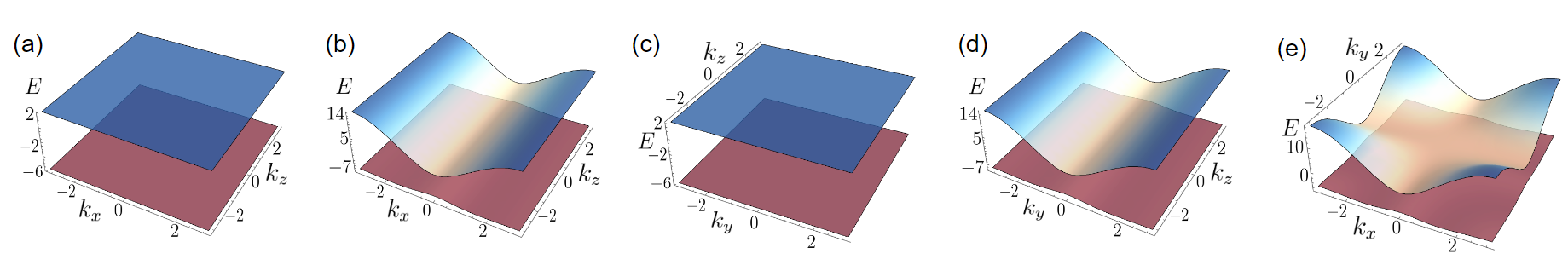
Figure 3: Energy spectrum of Eq. (5) for a) $k_{y}=0$, b) $k_{y}=2$, c) $k_{x}=0$, d) $k_{x}=2$, and e) any $k_{z}$ planes for $h=-(t_{a}-t_{b})=2t_{2}$, $4t^{\prime}=-(t_{a}+t_{b})$, $h=-4$, $t^{\prime}=0.5$ and $t_{2}=-2$. As discussed in the main text, both the bands are exactly flat for $k_{x}=0$ and $k_{y}=0$ planes. In contrast, for other 2D plane (any $k_{z}$) one of the bands become dispersive while the other becomes nearly flat.

Construction of non-trivial flat bands in 3D: To construct a three-dimensional insulator with non-trivial flat bands, we can simply stack several layers of the 2D Chern insulators with weak nearest-neighbor interaction ($t_{3}$). This adds a term $2\,t_{3}\cos k_{z}$ with $\sigma_{z}$ in Eq. (3). As $t_{3}$ increases, the flatness gradually diminishes although the bulk spectrum maintains a gap with nontrivial Chern number in $k_{x}-k_{y}$ plane. At $t_{3}/h=\pm\frac{1}{2}$, the bulk gap closes and a trivial metallic phase is obtained. Indeed, this is a trivial construction of 3D insulators with flat bands exhibiting only Chern invariant.

In contrast, we now provide a genuinely 3D lattice model which exhibits flat bands with both Chern and 3D Hopf invariants. To construct such a 3D lattice, we allow non-identical orbital hopping between next-nearest-neighbor in two different planes in contrast to the 2D case discussed earlier. The schematic of such construction is illustrated in Fig. (2). Note that we retain NN and NNN hopping between similar orbitals with similar strength in the $x-y$ plane as in 2D case. This leaves $d_{0}({\bf k})$ invariant. In the planes $x-z$ and $y-z$, the orbital-flipping NN terms of the previous 2D lattice act as NNN hopping. The momentum space Hamiltonian for such a 3D lattice construction reads off

$$H_{\textrm{3}D}(\textbf{k})=d_{0}(\textbf{k})\mathbb{1}+d_{x}(\textbf{k})\sigma_{x}+d_{y}(\textbf{k})\sigma_{y}+d_{x}(\textbf{k})\sigma_{z},$$ (4)

where $k=(k_{x},k_{y},k_{z})$ is a 3D crystal momentum; $d_{0}(\textbf{k})$ is same as before, however $d_{i}(\textbf{k})$s ($i\in\{x,y,z\}$) are modified as $d_{x}(\textbf{k})=2t_{2}(\sin k_{x}\sin k_{z}+\cos k_{z}\sin k_{y})$, $d_{y}(\textbf{k})=2t_{2}(-\sin k_{y}\sin k_{z}+\cos k_{z}\sin k_{x})$, $d_{z}(\textbf{k})=(h+(t_{a}-t_{b})(\cos k_{x}+\cos k_{y}))+2t_{3}\cos k_{z}$, due to the presence of hopping matrix elements along the $k_{z}$ direction. We note that the form of the 3D lattice model Hamiltonian has similar momentum structure (except a few other terms in the current model) with the rotated 2D Chern insulator introduced by Kennedy[4], where rotation is along the $z$ direction and the third momentum $k_{z}$ plays the role of angle of rotation. It is important to note that such a construction of 3D insulators by rotation may not be a generic construction, particularly for arbitrary Chern phases and it requires a detailed investigation in its own right.

Next, we investigate the presence of flat bands in $H_{3D}$. Notice that although $d_{x}({\bf k})$ and $d_{y}({\bf k})$ individually depends on $k_{z}$, the square of their sum $d_{x}({\bf k})^{2}+d_{y}({\bf k})^{2}$ is independent of $k_{z}$. The $k_{z}$ dependence enters in the spectrum only through $t_{3}$ term in $d_{z}({\bf k})$. However, for $t_{3}\ll t_{a},t_{b},t^{\prime},t_{2}$, the bands are nearly flat along $k_{z}$ and dispersive only along $k_{x}$ and $k_{y}$ for a particular configuration of parameters. For simplicity, we set $t_{3}=0$, and this simplifies energy spectrum in the $k_{y}=0$ plane as

$$E(k_{x},0,k_{z})= (t_{a}+t_{b})+(t_{a}+t_{b}+4t^{\prime})\cos(k_{x})$$

$$\pm\left[h^{2}+\frac{3}{2}(t_{a}-t_{b})^{2}+2t_{2}^{2}+2h(t_{a}-t_{b})\right.$$

$$+\frac{1}{2}(t_{a}-t_{b}-2t_{2})(t_{a}-t_{b}+2t_{2})\mbox{cos}(2k_{x})$$

$$\left.+2(t_{a}-t_{b})(t_{a}-t_{b}+h)\mbox{cos}(k_{x})\right]^{1/2}.$$ (5)

Remarkably, for the same flatness conditions in the 2D case, we obtain exact flat bands (see Fig. 3a) with energies

$$E(k_{x},k_{z})=(t_{a}+t_{b})\pm h.$$ (6)

For $k_{y}\neq 0$ planes, one of the bands becomes dispersive while the other one remains nearly flat as shown in Fig. (3)b. This also applies to $k_{x}=0$ and $k_{x}\neq 0$ planes. Fig.  (3c-d) demonstrates these features. In contrast to $k_{x}=0$ and $k_{y}=0$ planes, we obtain one band nearly flat in any $k_{z}$ planes with the same parameter discussed in the 2D case. The corresponding plots are shown in Fig. (3e). We note that for finite but small $t_{3}$, the flatness of the bands retains.

Topological Invariant: Having flat bands in a genuinely 3D cubic lattice model, we now characterise these flat bands either by topological Chern invariant or by Hopf invariant. We first compute Chern number $C$ for different flat bands discussed in the preceding sections. While flat bands in the $y-z$ and $x-z$ planes carry zero Chern number irrespective of the values of the parameters of the Hamiltonian, the flat band in the $x-y$ plane has finite Chern number similar to the 2D case discussed before. Thus the 3D model possesses a finite Chern number in the $x-y$ plane.

We now find if such a 3D model can host 3D Hopf invariant. To measure it, we introduce a Bloch sphere for the Hamiltonian $H_{\textrm{3}D}={\bf d({\bf k})}\cdot{\bf\sigma}$ in Eq. (4). The first term $d_{0}(\textbf{k})$ configures only the band spectrum but has nothing to do in classifying the topology of the system. Here for every k-point in the 3D Hamiltonian, we can identify a specific Bloch vector on the unit sphere defined as, $\hat{\textbf{d}}_{\textbf{k}}=\textbf{d}(\textbf{k})/|\textbf{d}(\textbf{k})|$. Any unit vector in the spherical-polar coordinate can generically be written in terms of azimuthal ($\phi$) and polar ($\theta$) angle by

$$\hat{\textbf{d}}_{\textbf{k}}=(\sin(\theta_{\textbf{k}})\cos(\phi_{\textbf{k}}),\ sin(\theta_{\textbf{k}})\sin(\phi_{\textbf{k}}),\cos(\theta_{\textbf{k}})).$$ (7)

The 3D Brillouin zone (BZ) can be identified as a 3-torus ($\textbf{T}^{3}$) and Bloch sphere of unit radius ($\hat{\textbf{d}}_{\textbf{k}}$) as 2-sphere ($\textbf{S}^{2}$). Following Ref. [17], we define a map $f:\textbf{T}^{3}\rightarrow\textbf{S}^{2}$. Note that there is a dimensional reduction between the initial and final manifold space. This implies there exists a one-dimensional sub-manifold in BZ for the preimage $f^{-1}(s)$, where $s\in\textbf{S}^{2}$ is a zero-dimensional point on the Bloch Sphere. For any two point $s_{1},s_{2}\in\textbf{S}^{2}$, the linking number between the preimage $f^{-1}(s_{1})$ and $f^{-1}(s_{2})$ is related with the Hopf Index of the system.

To visualize this, we consider two antipodal points $s_{1}=(1/\sqrt{2},1/\sqrt{2},0)$ and $s_{2}=(-1/\sqrt{2},-1/\sqrt{2},0)$ from Bloch sphere in its equatorial plane($\theta_{\textbf{k}}=\pi/2$) as shown in Fig. (4). The simultaneous solution of the three equations

$$\{d_{x}({\bf k}),d_{y}({\bf k}),d_{z}({\bf k})\}=\{\frac{1}{\sqrt{2}},\frac{1}{\sqrt{2}},0\}$$ (8)

for the point $s_{1}$ gives a one-dimensional submanifold in the BZ. The red line in Fig. (4) shows the solution and its $\epsilon$-neighbourhood for $f^{-1}(s_{1})$, where $\epsilon\ll 0.1$ and $|f^{-1}(s_{1})_{plot}|-|f^{-1}(s_{1})_{exact}|\leq\epsilon$. Similarly, if we solve for point $s_{2}$ and plot the blue line, it is observed that one line winds around other once. This implies the magnitude of Hopf index is 1.

Figure 4: a) Plot of Bloch sphere with unit radius. Red and blue points represent $s_{1}$ and $s_{2}$ as discussed in the main text. These two points are equated with the ${\bf d({\bf k})}$ to find the solution ${\vec{k}}$. The solutions are then plotted in (b). The parameters are same as in Fig. 1b.

Phase diagram:- Equipped with the computation of Hopf invariant, we now chart out the phase diagram of the Hamiltonian in Eq. (4). Fig. (5) illustrates several distinct phases in the parameter space $t_{2}$ and $(t_{a}-t_{b})$ with $h=-4$, $t^{\prime}=0.5$ and $(t_{a}+t_{b})=-2$. Evidently, the Hopf-Chern phases appear symmetrically in the $t_{2}$-$(t_{a}-t_{b})/2$ plane. For $2|(t_{a}-t_{b})|>|h|$, we find insulating phase with finite 3D Hopf and 2D Chern invariants. Otherwise, we obtain trivial insulating phase. At the transition point i.e, $(t_{a}-t_{b})=\pm h/2$ (vertical red colored line in Fig. (5)), the band gap closes at a single $k$ point in the BZ. In the non-trivial regime, the flat bands appear only at a special configuration of parameters (blue region) as indicated in Fig. (5). It is worth pointing out that the trivial insulating regime may also host flat bands in different planes. For a more weaker orbital-flipping NNN hopping $t_{2}=0.5$, the nearly flat band with a flatness $\sim 1/21$ of band gap in plane $k_{x}\sim 1$ or $k_{y}\sim 1$ is obtained for the parameters $h=-4$, $t^{\prime}=0.5$, $(t_{a}+t_{b})=-2$ and $(t_{a}-t_{b})=\pm 0.6$. This is denoted by dark green dots in the phase diagram.

Figure 5: Phase diagram of 3D Hamiltonian in the plane $t_{2}$-$(t_{a}-t_{b})/2$ with $h=-4$, $t^{\prime}=0.5$ and $(t_{a}+t_{b})=-2$. Note that the Hopf-Chern phases are symmetric with respect to $(t_{a}-t_{b})=0$. The bulk spectrum closes at red colored line. The blue dot represents parameters for having flat bands in the Hopf-Chern phase whereas the dark green dots represent parameters for flat bands in the trivial insulating regime.

Higher Chern model and Hopf Invariant: We next construct a 3D Hopf model which exhibits higher Chern phases with only NN and NNN as before. We take $t^{\prime}_{AA}=-t_{BB}=t^{\prime}$ in Eq. (2). This leads to $d_{0}(k)=(t_{a}+t_{b})(\cos k_{x}+\cos k_{y})$ and $d_{z}(k)=(h+(t_{a}-t_{b})(\cos k_{x}+\cos k_{y}))+4t^{\prime}\cos k_{x}\cos k_{y}$. $d_{x}$ and $d_{y}$ remain same as before. For $t_{a}=t_{b}$, the model exhibits Chern phases with $C=2$ for $-4<h<4$. With this, the 3D model can be constructed following the same procedure discussed in the preceding sections. To find Hopf invariant, the preimages of two antipodal points on the Bloch sphere are shown in Fig. (6c) for $h=-1$, $t^{\prime}=1$, $t_{2}=-2$ and $t_{a}=t_{b}=1$. Evidently, there is a winding between the two preimages, confirming a 3D model of both Hopf and higher Chern invariants with NN and NNN hopping. Moreover, the presence of two loops indeed indicates the two gaped Dirac points in the spectrum responsible for $C=2$ phase. It is worth pointing out that finding Hopf invariant in a higher Chern model is subtle and somewhat it depends on the location of Dirac point within the BZ. For example, the winding of preimages turns out to be easily identifiable in a Chern model with gaped Dirac points at the center of the BZ. In contrast, Chern models with gaped Dirac nodes at arbitrary momenta often give solutions for preimages for which number of winding is not easy to count. Hence, a better diagnostic is required which is beyond the scope of the current work.

We further comment if such a 3D Hopf-Chern model can host flat bands. Evidently, $d_{0}$ is now a constant parameter as $t_{a}$ and $t_{b}$ are fixed to allow only $C=2$ phase in the 2D model in Eq. (3). Consequently, the 3D model does not support flat bands along all the high-symmetric points in the BZ as evident in Fig. (6). For comparison, we have also added band spectrum for $C=1$. To get flat bands in such a 3D model, we must incorporate higher-order hopping which seems to be a natural choice (we do not present here for simplicity). Thus, finding flat bands in a higher Chern-Hopf model with NN and NNN neighbor is not guaranteed.

Figure 6: a) Bulk band spectrum along the high symmetric points in the cubic BZ (b) for both $C=1$ and $C=2$ phases. The parameters for the $C=2$ phase are taken to be $h=-1$, $t_{a}=t_{b}=1$, $t^{\prime}=1$, $t_{2}=-2$ and for $C=1$ phase we use parameters as in Fig. 3. c) The winding of preimages in the Hopf-Chern model with Chern number $C=2$.

Conclusion: In conclusion, we study flat bands with non-trivial Hopf and Chern number in a 3D lattice model. We show that such a lattice model exhibiting Hopf number can be constructed from a 2D Chern insulator. Depending upon the parameters of the model Hamiltonian and crystal planes, completely or nearly flat bands are obtained. We further show that a 3D Hopf model with higher Chern number is realizable with only NN and NNN hopping similar to the $C=1$ model, but the presence of flat bands in all crystal planes is not guaranteed. We point out that it is indeed an open problem to explore if any Chern model with arbitrary Chern number can be converted to a Hopf model with flat bands. This requires further investigation.

The lattice model proposed here is expected to be realizable in three-dimensional optical lattices of dipolar interacting spins. It has already been proposed that the standard Hopf insulators can be realized in polar molecules loaded in 3D optical lattices where dipolar interaction can be tuned to implement various hopping[58, 59]. In addition, Hopf model has been shown to be realizable in a circuit[13]. Since the proposed set up in the current work requires only short range hopping than the standard Hopf model[2], we believe that the flat bands and related Hopf physics can easily be achieved in 3D optical lattices with dipolar interaction and in an electric circuit.

Acknowledgement: We thank Shamik Banerjee for useful discussion.

References

- Fu and Kane [2007] L. Fu and C. L. Kane, Phys. Rev. B 76, 045302 (2007).
- Moore et al. [2008] J. E. Moore, Y. Ran, and X.-G. Wen, Phys. Rev. Lett. 101, 186805 (2008).
- Deng et al. [2013] D.-L. Deng, S.-T. Wang, C. Shen, and L.-M. Duan, Phys. Rev. B 88, 201105(R) (2013).
- Kennedy [2016] R. Kennedy, Phys. Rev. B 94, 035137 (2016).
- Liu et al. [2017] C. Liu, F. Vafa, and C. Xu, Phys. Rev. B 95, 161116(R) (2017).
- Alexandradinata et al. [2021] A. Alexandradinata, A. Nelson, and A. A. Soluyanov, Phys. Rev. B 103, 045107 (2021).
- Zhu et al. [2021] P. Zhu, T. L. Hughes, and A. Alexandradinata, Phys. Rev. B 103, 014417 (2021).
- Yan et al. [2017] Z. Yan, R. Bi, and Z. Wang, Phys. Rev. Lett. 118, 147003 (2017).
- Xu et al. [2022] P. Xu, W. Zheng, and H. Zhai, Phys. Rev. B 105, 045139 (2022).
- Lapierre et al. [2021] B. Lapierre, T. Neupert, and L. Trifunovic, Phys. Rev. Res. 3, 033045 (2021).
- Nelson et al. [2022] A. Nelson, T. Neupert, A. Alexandradinata, and T. c. v. Bzdušek, Phys. Rev. B 106, 075124 (2022).
- Yuan et al. [2017] X.-X. Yuan, L. He, S.-T. Wang, D.-L. Deng, F. Wang, W.-Q. Lian, X. Wang, C.-H. Zhang, H.-L. Zhang, X.-Y. Chang, and L.-M. Duan, Chinese Physics Letters 34, 060302 (2017).
- Wang et al. [2023a] Z. Wang, X.-T. Zeng, Y. Biao, Z. Yan, and R. Yu, Phys. Rev. Lett. 130, 057201 (2023a).
- Chang et al. [2017] G. Chang, S.-Y. Xu, X. Zhou, S.-M. Huang, B. Singh, B. Wang, I. Belopolski, J. Yin, S. Zhang, A. Bansil, H. Lin, and M. Z. Hasan, Phys. Rev. Lett. 119, 156401 (2017).
- Hu et al. [2020] H. Hu, C. Yang, and E. Zhao, Phys. Rev. B 101, 155131 (2020).
- Zhou et al. [2018] Y. Zhou, F. Xiong, X. Wan, and J. An, Phys. Rev. B 97, 155140 (2018).
- Yu [2019] J. Yu, Phys. Rev. A 99, 043619 (2019).
- Deng et al. [2018] D.-L. Deng, S.-T. Wang, K. Sun, and L.-M. Duan, Chinese Physics Letters 35, 013701 (2018).
- He and Chien [2020] Y. He and C.-C. Chien, Phys. Rev. B 102, 035101 (2020).
- Schuster et al. [2019] T. Schuster, S. Gazit, J. E. Moore, and N. Y. Yao, Phys. Rev. Lett. 123, 266803 (2019).
- Ezawa [2017] M. Ezawa, Phys. Rev. B 96, 041202(R) (2017).
- Wang et al. [2023b] Y. Wang, A. C. Tyner, and P. Goswami, Fundamentals of crystalline hopf insulators (2023b), arXiv:2301.08244 [cond-mat.mes-hall] .
- Leng and Van [2022] B. Leng and V. Van, Optics Letters 47, 5128 (2022).
- Cook and Moore [2022] A. M. Cook and J. E. Moore, Communications Physics 5, 262 (2022).
- Ünal et al. [2019] F. N. Ünal, A. Eckardt, and R.-J. Slager, Phys. Rev. Res. 1, 022003(R) (2019).
- Yue and Liu [2023] Y.-G. Yue and Z.-X. Liu, Phys. Rev. B 107, 045130 (2023).
- Graf and Piéchon [2022] A. Graf and F. Piéchon, Multifold hopf semimetals (2022), arXiv:2203.09966 [cond-mat.mes-hall] .
- Ünal et al. [2020] F. N. Ünal, A. Bouhon, and R.-J. Slager, Phys. Rev. Lett. 125, 053601 (2020).
- Goda et al. [2006] M. Goda, S. Nishino, and H. Matsuda, Phys. Rev. Lett. 96, 126401 (2006).
- Chalker et al. [2010] J. T. Chalker, T. S. Pickles, and P. Shukla, Phys. Rev. B 82, 104209 (2010).
- Niţă et al. [2013] M. Niţă, B. Ostahie, and A. Aldea, Phys. Rev. B 87, 125428 (2013).
- Nishino et al. [2003] S. Nishino, M. Goda, and K. Kusakabe, Journal of the Physical Society of Japan 72, 2015 (2003), https://doi.org/10.1143/JPSJ.72.2015 .
- Kimura et al. [2002] T. Kimura, H. Tamura, K. Shiraishi, and H. Takayanagi, Phys. Rev. B 65, 081307(R) (2002).
- Pollmann et al. [2008] F. Pollmann, P. Fulde, and K. Shtengel, Phys. Rev. Lett. 100, 136404 (2008).
- Leykam et al. [2013] D. Leykam, S. Flach, O. Bahat-Treidel, and A. S. Desyatnikov, Phys. Rev. B 88, 224203 (2013).
- Flach et al. [2014] S. Flach, D. Leykam, J. D. Bodyfelt, P. Matthies, and A. S. Desyatnikov, Europhysics Letters 106, 19901 (2014).
- Bodyfelt et al. [2014] J. D. Bodyfelt, D. Leykam, C. Danieli, X. Yu, and S. Flach, Phys. Rev. Lett. 113, 236403 (2014).
- Danieli et al. [2015] C. Danieli, J. D. Bodyfelt, and S. Flach, Phys. Rev. B 91, 235134 (2015).
- Ramachandran et al. [2017] A. Ramachandran, A. Andreanov, and S. Flach, Phys. Rev. B 96, 161104(R) (2017).
- Khomeriki and Flach [2016] R. Khomeriki and S. Flach, Phys. Rev. Lett. 116, 245301 (2016).
- Vicencio et al. [2015] R. A. Vicencio, C. Cantillano, L. Morales-Inostroza, B. Real, C. Mejía-Cortés, S. Weimann, A. Szameit, and M. I. Molina, Phys. Rev. Lett. 114, 245503 (2015).
- Mukherjee et al. [2015] S. Mukherjee, A. Spracklen, D. Choudhury, N. Goldman, P. Öhberg, E. Andersson, and R. R. Thomson, Phys. Rev. Lett. 114, 245504 (2015).
- Apaja et al. [2010] V. Apaja, M. Hyrkäs, and M. Manninen, Phys. Rev. A 82, 041402(R) (2010).
- Wu et al. [2007] C. Wu, D. Bergman, L. Balents, and S. Das Sarma, Phys. Rev. Lett. 99, 070401 (2007).
- Hwang et al. [2021] Y. Hwang, J.-W. Rhim, and B.-J. Yang, Phys. Rev. B 104, 085144 (2021).
- Sun et al. [2011] K. Sun, Z. Gu, H. Katsura, and S. Das Sarma, Phys. Rev. Lett. 106, 236803 (2011).
- Tang et al. [2011] E. Tang, J.-W. Mei, and X.-G. Wen, Phys. Rev. Lett. 106, 236802 (2011).
- Neupert et al. [2011] T. Neupert, L. Santos, C. Chamon, and C. Mudry, Phys. Rev. Lett. 106, 236804 (2011).
- Yang et al. [2012] S. Yang, Z.-C. Gu, K. Sun, and S. Das Sarma, Phys. Rev. B 86, 241112(R) (2012).
- Goldman et al. [2011] N. Goldman, D. F. Urban, and D. Bercioux, Phys. Rev. A 83, 063601 (2011).
- Chen et al. [2012] W.-C. Chen, R. Liu, Y.-F. Wang, and C.-D. Gong, Phys. Rev. B 86, 085311 (2012).
- Bergman et al. [2008] D. L. Bergman, C. Wu, and L. Balents, Phys. Rev. B 78, 125104 (2008).
- Pal and Saha [2018] B. Pal and K. Saha, Phys. Rev. B 97, 195101 (2018).
- Graf and Piéchon [2021] A. Graf and F. Piéchon, Phys. Rev. B 104, 195128 (2021).
- Paananen and Dahm [2015] T. Paananen and T. Dahm, Phys. Rev. A 91, 033604 (2015).
- Sitte et al. [2013] M. Sitte, A. Rosch, and L. Fritz, Phys. Rev. B 88, 205107 (2013).
- Weeks and Franz [2012] C. Weeks and M. Franz, Phys. Rev. B 85, 041104(R) (2012).
- Schuster et al. [2021a] T. Schuster, F. Flicker, M. Li, S. Kotochigova, J. E. Moore, J. Ye, and N. Y. Yao, Phys. Rev. Lett. 127, 015301 (2021a).
- Schuster et al. [2021b] T. Schuster, F. Flicker, M. Li, S. Kotochigova, J. E. Moore, J. Ye, and N. Y. Yao, Phys. Rev. A 103, 063322 (2021b).