What’s the Problem, Linda?
The Conjunction Fallacy as a Fairness Problem

Abstract.

Artificial Intelligence (AI) researchers increasingly focus on creating automated decision-making (ADM) systems that operate close to human-like intelligence. Such efforts have pushed AI researchers into cognitive fields like psychology. As a result, the works of Daniel Kahneman and the late Amos Tversky on biased human decision-making, including the study of the conjunction fallacy, have experienced a second revival. Under the conjunction fallacy a human decision-maker goes against basic probability laws and ranks as more likely a conjunction over one of its parts. It has been proven overtime through a set of experiments with the Linda Problem being the most famous one. Although this interdisciplinary effort is welcomed, we fear that AI researchers ignore the driving force behind the conjunction fallacy as captured by the Linda Problem: the fact that Linda must be stereotypically described as a woman. In this paper, we revisit the Linda Problem and formulate it as a fairness problem. We introduce perception as a parameter of interest through the structural causal perception framework. Using an illustrative decision-making example, we showcase the proposed conceptual framework and its potential impact for developing fair ADM systems.

1. Introduction

The works by psychologists Daniel Kahneman and Amos Tversky have been influential in building our understanding of human decision-making. We now know that humans resort to mental shortcuts or heuristics that enable faster but potentially biased decisions (Tversky and Kahneman, 1974). Heuristics are shaped by each individual’s experience. The situation in which two individuals interpret differently the same information or perception is a consequence of these cognitive processes. The narrative on humans being inconsistent, unreliable, and opaque decision-makers (Kahneman et al., 2016, 2021) is another consequence.

Kahneman and Tversky’s work has had a considerable interdisciplinary impact. Their findings, for instance, challenged the rational agent models that once dominated economic theory and fueled the rise of Behavioral Economics or “nudging” (Thaler and Sunstein, 2008). Kahneman received the 2002 Nobel Prize in Economics (Tversky passed away in 1996). This is no minor achievement. Economics, arguably the most influential field in governance since the Great Depression (Appelbaum, 2019), is an insular social science (Pieters and Baumgartner, 2002; Fourcade et al., 2015; Hamermesh, 2018) known for its preference to describe complex human behavior with well-behaved mathematical formulas, a preference often dubbed as “physics envy” (Nelson, 2015; Skidelsky, 2019).

Their work (though, mostly Kahneman’s at this point) has started to influence Artificial Intelligence (AI), another field with an interest in modeling human behavior in precise and predictable ways. Yoshua Bengio, 2018 Turing Award and prominent AI researcher, for example, proposed in 2019 a System 1 and System 2 for deep learning models (Bengio, 2019) based on Kahneman’s bestselling book, Thinking, Fast and Slow (Kahneman, 2011). The fact that Kahneman himself was invited as a speaker to NeurIPS 2021 (Kahneman, 2021), a leading AI conference, is another example. This trend is unsurprising. There is a genuine push from the AI community to use Kahneman and Tversky’s work to create systems that can operate like, learn from, and improve over human-like intelligence (e.g., (Booch et al., 2021)). Unfortunately, those same findings that put into question human capabilities also help motivate an unchecked AI-hype that ignores its societal impact (e.g., (Crawford, 2021)). We should expect Kahneman and Tversky’s work to continue becoming more influential within AI.

This paper hopes to raise awareness around this trend from a fairness perspective. We focus on one of Kahneman and Tversky’s most famous experiments, the Linda Problem, which studies the conjunction fallacy. The conjunction fallacy occurs when the probability of a conjunction, $P$(Linda is a bank teller and Linda is an active feminist), is considered higher than the probability of one of its parts, $P$(Linda is a bank teller). It is caused by the representativeness heuristic. Under this heuristic, an event is made to be more representative of a class than what it actually is, measured by a higher probability, due to an individual’s perception of the event. We revisit the Linda Problem as a causal fairness problem, highlighting that the biased choice—as in the non-rational choice—of picking the conjunction over one of its parts says a lot about the need for handling better protected attributes like gender when building an automated decision-making (ADM) system. Granted, humans are not always preferred over an ADM (Miller, 2018). Still, it is dangerous to reduce the representativeness and other heuristics as processing flaws while ignoring what motivated an individual to form said heuristics in the first place. We believe the Linda Problem exhibits this tension.

Our contributions are twofold. First, we re-formulate the Linda Problem into a fairness problem with potential implications for ADM systems. Second, we propose the structural causal perception framework and study the role of perception as a fairness parameter. Overall, we contribute to a growing line of position papers (e.g., (Hu and Kohler-Hausmann, 2020; Hanna et al., 2020; Kasirzadeh and Smart, 2021; Lu et al., 2022; Alvarez and Ruggieri, 2023)) warning about using (or misusing) lightly insights from other fields for machine learning research.

The rest of this section covers the required background knowledge. Section 2 studies further the effectiveness of the Linda Problem; Section 3 presents the structural causal perception framework and revisits the Linda Problem with perception as a parameter; and Section 4 illustrates the proposed conceptual framework using a decision-making example. We conclude with the relevant related work in Section 5 and a discussion in Section 6.

1.1. Causal Graphs

Let an upper-case letter denote a random variable or class, and a lower-case letter denote its realization or instance. Hence, $P(X)$ represents the probability distribution of $X$ while $P(x)$ the probability that $X$ equals $x$. We use structural causal models (SCM) as popularized by Pearl (2009) as our modeling approach. SCM allow us to organize our assumptions about the random variables of a given problem in a convenient way that can also engage multiple stakeholders (Mulligan, 2022). Another reason we use SCM are their increasing popularity within AI research that aims to approximate human-like intelligence (Schölkopf, 2019; Schölkopf et al., 2021), which is often described in terms of causal reasoning (Pearl and Mackenzie, 2018).

SCM are a type of probabilistic graphical models in which each node represents a random variable and the directed edges between them, denoted by arrows, represent a causal relation. For instance, the causal graph $X_{1}\rightarrow X_{2}$ reads as “$X_{1}$ causes $X_{2}$” and describes a cause-effect or parent-child pair. Under SCM, the causal effect from parent(s) to child are modeled in terms of (structural) equations.

We define formally the SCM $\mathcal{M}$ with associated causal graph $\mathcal{G}$ for $p$ random variables $\{X_{1},\dots,X_{p}\}$ as the set of assignments $\{X_{i}:=f_{i}(X_{pa(i)},U_{i})\}_{i=1}^{p}$ where $f_{i}$ is a structural equation, $U_{i}$ a noise term, and $X_{pa(i)}$ the parents or direct causes of $X_{i}$. For simplicity, as we use the SCM $\mathcal{M}$ and causal graph $\mathcal{G}$ to revisit conceptually the Linda Problem, we assume $\mathcal{G}$ to be acyclic, $U_{i}$ to be independently distributed, and $f_{i}$ to be an additive noise model specification. These are standard assumption in the causal fairness literature (Makhlouf et al., 2020; Binkyte-Sadauskiene et al., 2022). The first assumption turns $\mathcal{G}$ into a directed acyclical graph (DAG), implying there are no feedback loops of information. The second assumption implies causal sufficiency, meaning there are no unaccounted common causes. And the third assumption implies an invertible function, allowing for the identifiability of causes (Peters et al., 2017).

We also define the adjacency matrix $\mathcal{P}$ associated to the DAG $\mathcal{G}$ as it is useful for communicating the causal graph structure. Let $\mathcal{P}$ be a $p\times p$ matrix with 0 or 1 entries. The $i$-row $j$-column element $p_{i,j}\in\mathcal{P}$ equals 1 if there exist a causal relation between $X_{i}$ and $X_{j}$: $X_{i}\rightarrow X_{j}$; otherwise, $p_{i,j}\in\mathcal{P}$ equals 0.

Under a SCM we can factorize the joint probability distribution of $\{X_{1},\dots,X_{p}\}$ as a product of the parent-child pairs:

(1) $$P(X_{1},\dots,X_{p})=\prod_{i=1}^{p}P\Big{(}X_{i}\,|\,X_{par(i)}\Big{)}$$

which motivates the DAG $\mathcal{G}$. See Appendix A for an illustrative example showcasing $\mathcal{M}$, $\mathcal{P}$, and $\mathcal{G}$.

1.2. The Conjunction Fallacy

For any two random variables $X_{1}$ and $X_{2}$, it holds that their intersection cannot be more probable than any of its parts: $P(X_{1}\cap X_{2})\leq P(X_{1})$ (or $P(X_{2})$). This rule is known as the conjunction rule and it comes from the basic qualitative laws of probability: the probability of what is contained cannot be more than the probability of what contains it. Therefore, we define the conjunction fallacy as the contradiction to the conjunction rule:

(2) $$P(X_{1}\cap X_{2})\;>\;P(X_{1})\;(\text{or}\,>\,P(X_{2}))$$

which holds regardless of whether $X_{1}$ and $X_{2}$ are independent. As with the conjunction rule, the conjunction fallacy follows for more than two random variables.

1.3. The Linda Problem

Kahneman and Tversky tested the conjunction fallacy (2) via a series of decision-making experiments (Tversky and Kahneman, 1981, 1983) in which participants were provided with several fictitious profiles and asked to rank the statements that best described each profile’s outcome in terms of the most probable. The Linda Problem, which we present below in its reduced form, remains the most famous of these profiles.

Definition 1.1 (The Linda Problem).

Linda is 31 years old, single, outspoken, and very bright. She majored in philosophy. As a student, she was deeply concerned with issues of discrimination and social justice, and also participated in anti-nuclear demonstrations. What is more probable today?

(a) Linda is a bank teller; or

(b) Linda is a bank teller and is active in the feminist movement.

The fallacy in Def. 1.1 occurred as participants in the experiments, including those with statistical training, overwhelmingly ranked the conjunction, option (b), over one of the conjunction’s parts, option (a). A “rational” or “unbiased” decision-maker should have been able to see through the conjunction fallacy.

2. What’s the Problem, Linda?

In popular imagination, she lives one or more several cliché-ridden narratives.

Women by Hilton Als

We study the effectiveness of the Linda Problem from a fairness perspective. As shown in (2), the conjunction fallacy is a probabilistic statement, which is usually how information is represented for and by ADM systems. What is interesting about the Linda Problem for our purposes is not that it illustrates irrational decision-making but that it does so by evoking a certain imagery of Linda. This is important as the fairness literature has consistently shown that human bias tends to precede AI bias (Angwin et al., 2016; Dastin, 2018; Heikkila, 2022; Ruggieri et al., 2023).

2.1. The Probabilistic Problem of Representation

The conjunction fallacy and, thus, the Linda Problem are driven by the representativeness heuristics, one of three judgment heuristics that can cause biased decision-making under uncertainty (Tversky and Kahneman, 1974). These heuristics refer to scenarios where humans, often unconsciously, apply shortcuts to reduce the complex task of making decisions via probabilistic reasoning. The representativeness heuristic is used in scenarios where we evaluate the degree to which one instance is representative of another instance. The Linda Problem is, in turn, a representation problem.

The representation problem dwells into the question of resemblance between instances (Tversky and Kahneman, 1974): the more one instance resembles another, the more representative it is of the other instance. Here, we talk about some degree of representativeness, which translates naturally into how we understand probabilities. The question “what is the probability that $a$ belongs to the class $A$?” implicitly asks “to what degree the instance $a$ resembles other known instances $a^{\prime}$ in the class $A$?”. If $a$ resembles $a^{\prime}\in A$, then we will judge the probability that $a$ belongs to $A$ or that $a$ is generated by $A$ to be high. Hence, the formulation $P(a\in A)\equiv P(A=a)$ is a statement of representation where $P$ summarizes our doubts around $a\in A$, or lack of certainty, into a number ranging between 0 and 1.

The question of resemblance behind the representation problem is not far from how a machine learning model approaches a classification task. Usually, we are interested in training a classifier $f$ using data that contains a set of features $X$ and a class $Y$. The resulting classifier outputs a predicted class based on the provided features, $f(X)=\hat{Y}$, judging how representative the inputs are of the data used for training it. If $f$ learned that $X=x^{\prime}$ has $Y=y$ and the new input $x$ resembles $x^{\prime}$, then $f(x)=y$ also.

Given the probabilistic nature of the problem of representation, it is not surprising that Kahneman and Tversky’s work made its way into AI research. In particular, what is implied by the ongoing AI work that borrows from cognitive psychology is that machine learning models represent an opportunity to move away from these heuristics and achieve an unbiased decision-maker. Such view has yet to be made explicit, but we argue that it is implied by, one, the narrative that humans are not reliable decision-makers relative to algorithms (Kahneman et al., 2016; Miller, 2018; Kahneman et al., 2021) and, two, the belief that AI will eventually be capable of imitating human-like intelligence (Bengio, 2019; Booch et al., 2021). Under this premise, a classifier should be able to overcome issues like the conjunction fallacy, seeing right trough the Linda Problem.

We view the existence of a narrative within AI in which algorithms represent the rational agent in this next phase of modeling human decision-making. In fact, it could be argued that algorithms represent the rational agents economists once envisioned in their theoretical models before these judgment heuristics disproved the field’s dominant narrative. Like the homo economicus, algorithms minimize the expected loss (or maximize the expected utility) as defined by an objective function; like the homo economicus, algorithms rationalize the world via probabilities; like the homo economicus, algorithms consistently derive the same answer under the same information; and so on.

A key difference, however, is that Economics, as a social science, could not ignore the dissimilarities between the rational agents in its models and its real-world human subjects; AI instead, as a science interested in the social, can for now focus on developing the algorithms that embrace these dissimilarities under the promise of a new and improved rational agent. We note that this is a legitimate and potentially beneficial goal as human judgment can be flawed (e.g., (Kahneman, 2011)). Our position is that, when drawing from these judgment heuristics for designing better ADM systems, we must acknowledge the social and cultural drivers behind them.

2.2. The Implicit Protected Attribute

We define perception as having different representations for the same information (Kahneman, 2021). Perception leads to the problem of misrepresentation. In the case of the Linda Problem, individuals found Linda to be more representative of a bank teller and an active feminist than just a bank teller, despite the violation of the conjunction rule. What determines the degree of representativeness in the representativeness heuristic varies across individuals. In the Linda Problem respondents were essentially asked whether Linda, based on her description, resembles more a bank teller or an active feminist bank teller. Here, perception triumphed over basic probability laws: something in Linda’s description elicited a representation of her that made the active feminist bank teller statement more likely despite the conjunction fallacy.

This is the whole point of the Linda Problem: to illustrate how the way humans determine resemblance affects human judgement. Kahneman and Tversky purposely wrote Linda’s profile to be representative of an active feminist and unrepresentative of a bank teller (Tversky and Kahneman, 1983), eliciting the biases of the participants through the representativeness heuristics that led them to choose the least likely option. Only Linda is described in the Linda Problem. The meanings behind what represents a bank teller and an active feminist needed to be incorporated somehow into the problem by the participants. This is “data” that is not provided by the problem, yet it is clearly relevant to it.

Kahneman and Tversky relied on building a prototype of Linda that would resonate with known stereotypes of women like Linda at the time. For instance, the reference to anti-nuclear protests illustrates a problem that was written for people that experienced the Cold War era and the overall chaos of the 60s, such as the student demonstrations in US colleges and student protests in cities like Paris and Prague that took place in the late 1960s.

Linda is described as female, meaning that she is an instance of the class gender. Gender, a common protected attributed along with race, plays a role in eliciting the representations of the respondents in the Linda Problem. Gender is considered a social category. Social categories are the result of classifying people and allocating them into groups over shared perceived identities. It is a common human trait as classification systems are embedded in society, historically upheld, and uncontested (Bowker and Star, 1999). Gender is also considered a social construct. Social constructs refer to categorization practices meant to classifyand divide individuals for enforcing, for example, exclusionary policies (Mallon, 2007; Hu and Kohler-Hausmann, 2020; D’Ignazio and Klein, 2020).

Overall, Linda represents some type of female instance(s) of the class gender meant to resonate with the respondents, or a stereotype. Stereotypes, as the ones used for Linda’s description in the problem, are products of social categorization. The concept itself refers to the cognitive representation people develop about a particular social category, based around beliefs and expectations about probable behaviors, features and traits (Beukeboom and Burgers, 2019). For stereotypes to become social phenomena, the perceived collection of expected behaviours, features or traits about particular group of people must transcend individual mental processes, and be shared and maintained among large groups of people (Beukeboom and Burgers, 2019).

Stereotypes, or the representations the individual harbours toward certain groups (Johnson, 2020), can translate into implicit and explicit attitudes that materialize into bias. It is this social kind of bias that mainly motivates fair machine learning today. Forming such biases seems inherently human. Unsurprisingly, some solutions to mitigate these biases focus more on the none human aspects, like developing an algorithm, rather than the human origins of the problem, like our societies and culture. Consider, for instance, that the effectiveness of the Linda Problem to showcase the conjunction fallacy clearly lies on a well-thought-out description of Linda by Kahneman and Tversky based on female stereotypes. The role of the protected attribute in Def. 1.1 is similar to that in fair machine learning where the rational algorithm can make biased decisions due to the observed or latent influence of protected attributes like gender.

Similar to the critique by Hu and Kohler-Hausmann (2020) on fair machine learning research, it is important for AI researchers using the judgment heuristics to state the ontological assumptions of the problem. It is appealing to dismiss the conjunction fallacy as a mistake, an error of judgment, but the fact that the Linda Problem has continued to prove this fallacy might signal a shared social phenomenon that needs to be interpreted meaningfully if we are to use it for training algorithms. We believe there is the need to be more explicit on why Linda elicits such irrational responses. As we view it, the main concern with the Linda Problem is not that it proves the conjunction fallacy and, in turn, our own potential irrationality, but that it takes a Linda to make us irrational.

2.3. As a Causal Problem

We setup Def. 1.1 under the structural causal models (SCM) introduced in Section 1.1. Let $A$ denote the instance where Linda is a bank teller, $B$ denote the instance where Linda is an active feminist, and $M$ represent Linda’s description or the model as referred to by Tversky and Kahneman (1983). We treat all three as random variables and compare the two statements of the Linda Problem, (a) Linda is a bank teller and (b) Linda is a bank teller and an active feminist, in terms of probability distributions:

$$\text{{(a)}}\;P(A) vs.\ \text{{(b)}}\;P(A\cap B) =P(A|B)\cdot P(B)$$

(3) $$=P(B|A)\cdot P(A)$$

$$=P(B)\cdot P(A)\;\;\text{if}\;A\perp\!\!\!\perp B$$

where we factorize the conjunction into three possible factorizations using Bayes’s Theorem. The third factorization occurs when $A$ and $B$ are independent but not mutually exclusive instances, meaning that they can occur simultaneously but without affecting each other. The model $M$ is “integrated out” from the statements as it is omnipresent: both statements or narratives respond to the same information. Formally, we mean $P(A)=\int_{M}P(A|M)\cdot P(M)$ and $P(A\cap B)=\int_{M}P(A,B|M)\cdot P(M)$, which we avoid including in (2.3) to avoid notation cluttering.

To construct the SCM $\mathcal{M}$ and DAG $\mathcal{G}$ for the Linda Problem we must choose one possible factorization for the conjunction—statement (b) in (2.3)—as the causal graph needs to represent a unique or faithfull factorization of the distribution (Peters et al., 2017). Using (1) we write the three options as shown in (2.3): $A\rightarrow B$; $B\rightarrow A$; and $A\,B$ where the arrow denotes the causal relation. We can interpret $A\rightarrow B$ as ‘being a bank teller causes Linda to be active in the feminist movement” while $B\rightarrow A$ as “being active in the feminist movement causes Linda to work as a bank teller”. Similarly, $A\,B$ means that there is no causal link between being a bank teller and active in the feminist movement. All three are equally plausible under $P(A\cap B)$.

We focus on the second option, $B\rightarrow A$, because it allows us to better compare the statements (a) and (b), where the latter differs from the former only by the term $P(B|A)$. We view this term as a sort of adjustment mechanism that shapes the marginal distribution $P(A)$. Our choice for this factorization of the conjunction is based solely on the additional term $P(B|A)$ that differentiates statement (b) from statement (a). The analysis we present in the next sections follows also for the other two factorizations.

Having picked our factorization for the conjunction, we construct the causal graphs for both statements or narratives in Figure 1 based on (1). We include Linda’s description or model $M$. This is because it was constructed by Kahneman and Tversky to elicit the representativeness heuristic along with the classes bank teller and active feminist. The causal graph highlights, structurally, the role of the model $M$ in the Linda Problem. While we marginalized $M$ in (2.3), we now include it explicitly in Figure 1. We could write (a) and (b) in (2.3), respectively, as $P(A|M)\cdot P(M)$ and $P(B|A\cap M)\cdot P(A|M)\cdot P(M)$ using Figure  1—both forms are equivalent.

Figure 1. The causal graphs of the Linda Problem for the statements (a) $P(A)$ or “Linda is a bank teller” (left) and (b) $P(B|A)\cdot P(A)$ or “Linda is a bank teller and an active feminist” (right), respectively, including the model $M$.

3. Perception as a Parameter

We motivate our proposed structural causal perception framework. It is a conceptual framework centered on formalizing the role of perception as a parameter for the fairness problem. Under this framework, we revisit the Linda Problem and use the notion of perception to formulate it, along with the conjunction fallacy, as a case of additional information that is being incorporated by the decision maker. Under Figure 1, can we explain how a respondent chooses (a) $P(A)$ over (b) $P(A\cap B)$ under the same description $M$? In other words, can we explain the conjunction fallacy under this causal formulation of the Linda Problem? Such is the goal of the proposed structural causal perception framework.

3.1. Senders and Receivers

We want to make perception, that is the act of interpreting the same information differently, operational. Despite revisiting Def. 1.1 in Section 2.3, the conjunction rule still holds. In Figure 1 a rational agent should be able to see that:

(4) $$P(A|M)\cdot P(M)\geq P(B|A\cap M)\cdot P(A|M)\cdot P(M)$$

or $P(A)\geq P(B|A)\cdot P(A)$. Hence, where is the elicited additional information coming from? As it is, structurally, we cannot account for the violation of the conjunction rule (4) for the random variables $A$, $B$, and $M$. To do so, borrowing from signaling games (Sobel, 2020) in Economics, we define two types of agents: the senders (S) who provide information about themselves and the receivers (R) who interpret such information. We view Linda (or the description of Linda) as S and the respondents that have to interpret the description of Linda as R. Therefore, we move away from the what you see is what you get (WYSIWYG) default setting when formulating fairness problems. We now allow the receivers to incorporate additional information into the problem through the act of interpretation that characterizes them. Note that here we only borrow from signaling games the notion of two agents, a sender and a receiver, exchanging information. We do not explore, for instance, the potential game theoretic implications, which remains for future work.

Definition 3.1 ($\delta$-adjustment).

From the point of view of a receiver R, we define the $\delta$-adjustment such that:

$$P(A\cap M)<g(\delta,P(A\cap B\cap M))$$

where $|\delta|\in[0,1]$ and $g$ denotes the functional form in which $\delta$ affects the probability distribution.

Def. 3.1 argues that for a receiver $\mathbf{R}$ to fall for the conjunction fallacy it must adjust the information it receives from the sender $\mathbf{S}$. Conceptually, the perception between the two agents toward $M$ differs by some $\delta$-adjustment that influences the ranking of the two statements about Linda. Formally and structurally, as formulated under Figure 1, this step would require $\delta$ to enter the structural equation as described by $g$. Here, we explore the scenario where $\delta$ enters linearly as it is simpler to interpret. See Appendix A for further details. This, in terms of probabilities, means that $\exists\;|\delta|\in[0,1]$ such that:

(5) $$P(A\cap M)<P(A\cap B\cap M)+\delta\leq 1$$

where we expect $A$ not to be certain, i.e., $P(A)=\int_{M}P(A|M)\cdot P(M)<1$. The focus here is more on the conceptualization of the $\delta$-adjustment. Def. 3.1 under the assumed $g$ highlights how we envision perception affecting a causal problem and violating the conjunction rule (4). Given our modeling setup under structural causal models, it is convenient to talk about structural adjustments as any $\delta$-adjustment can have a structural interpretation.

We are interested then in why and how the $\delta$-adjustment is motivated, derived, and applied by the receiver $\mathbf{R}$ based on the description of Linda by the sender $\mathbf{S}$. It is the description of Linda $M$ that elicits the representativeness heuristic. It should also be $M$ that evokes or “calls to mind” the $\delta$-adjustment by the receiver $\mathbf{R}$. Since we have framed this process as $\mathbf{S}$ sending information and $\mathbf{R}$ interpreting it, or a one-sided single stage signaling game, the act of evoking an adjustment falls solely on the receiver $\mathbf{R}$ as it did with the respondents in Kahneman and Tversky’s experiments. There is no verification step, for example, where $\mathbf{R}$ confirms its believes about the information provided by $\mathbf{S}$. It is possible to extend this setting in future work. Now we need to formalize how the receiver derives the $\delta$-adjustment based on $M$.

3.2. Categorization and Signification

We distinguish two processes, categorization and signification (Loury, 2019), that are involved in the act of interpreting protected attributes like genders. Categorization entails sorting instances into categories, or defining the attribute. Signification entails an interpretive act in which we represent the social meanings relevant to the decision context, or interpreting the attribute. For example, female, as in sorting an individual as a female or male, is a category while feminine, as in interpreting individual qualities with being female, is a signification.

Consider the description of Linda in Def. 1.1. We can deconstruct $M$ by writing down its elements or descriptors. In doing so, we answer the question what does it mean to be (or belong to the class) Linda? Based on the Linda Problem, to be Linda means (in no particular order) being: female, 31, single, outspoken, bright, a philosophy major, and active in social causes. In terms of structure, putting aside the causal for now, it means being able to zoom into the node $M$ in Fig. 1 and observe its internal components. It is similar to stating the ontological commitments of Linda (Hu and Kohler-Hausmann, 2020) with Linda being a class and Linda’s descriptors its properties (Gruber, 1995).

The same “zooming into” process could be done for being a bank teller, $A$, and being an active feminist, $B$; though, neither descriptions are provided by the sender $\mathbf{S}$. This means that these conceptualizations are up to the receiver $\mathbf{R}$. For instance, one receiver could describe a bank teller as task oriented, organized, and good with numbers. An individual described by said descriptors, will in turn increase his or her resemblance and thus increase the chances of being associated to the class bank teller. What constitutes $A$ and $B$ will vary by each individual $\mathbf{R}$.

3.3. Structural Causal Perception

We present three definitions: a representative receiver, a conceptualization mapping, and an operationalization mapping. The last two definitions define what we mean by having a receiver that is representative: what perceptions such receiver has (conceptualization) and how these are incorporated into the decision-making process (operationalization) define who or what the receiver represents. Together, these definitions constitute the structural causal perception framework.

Let us consider a given SCM $\mathcal{M}$ with associated DAG $\mathcal{G}$ and adjacency matrix $\mathcal{P}$. It embodies the WYSIWYG setting. Let $X_{i}$ represent a variable from a the set of $|X|=p$ variables. Using the adjacency matrix, let $\mathcal{P}_{i,.}$ represent all direct causes of $X_{i}$ (or children), meaning that for the $i^{th}$ row in $\mathcal{P}$ we focus on all $j^{th}$ column entries that equal to 1. Since $\mathcal{G}$ is a DAG, it follows that $p_{i,j}\in\mathcal{P}$ equals 0 when $i=j$ or when $X_{j}$ is not caused by $X_{i}$.

Definition 3.2 (Conceptualization mapping $\Omega$).

Let $\Omega(X_{i},\mathbf{R})$ denote the conceptualization mapping of a receiver $\mathbf{R}$. It associates the node $X_{i}$ in $\mathcal{G}$ (or variable in $\mathcal{M}$) to a list of descriptors pertaining to $X_{i}$ according to $\mathbf{R}$. We define a descriptor $\omega$ as an element of a given conceptualization $\Omega$. Conceptually, $\Omega(X_{i},\mathbf{R})$ answers to the question what descriptors does $\mathbf{R}$ associate with $X_{i}$?

Definition 3.3 (Operationalization mapping $\Psi$).

Let $\Psi(\mathcal{P}_{i,.},\mathbf{R})$ denote the operationalization mapping of a receiver $\mathbf{R}$. It provides the links or associations between the descriptors of the node $X_{i}$ in $\mathcal{G}$ (or variable in $\mathcal{M}$) with the descriptors of all other nodes (or variables) that are direct effects of $X_{i}$ according to $\mathbf{R}$. $\Psi$ follows the existing structure of the causal graph $\mathcal{G}$ and its adjacency matrix $\mathcal{P}$. Conceptually, $\Psi(\mathcal{P}_{i,.},\mathbf{R})$ answers to the question how does $\mathbf{R}$ relate the descriptors of the cause $X_{i}$ to the descriptors of its direct effects?

Both definitions are conceptual and can be formalized further for a specific application. The main implication derived from both definitions is that, under the structural causal perception framework, we allow for the agent making the decisions to incorporate additional information and enrich with it the information already provided by the problem. In practical terms, Def. 3.2 refers to when the individual enriches the information provided with their own information, such as when each participant in the Linda Problem had to provide an image of what constitutes an active feminist. Similarly, Def. 3.3 refers to when the individual links the additional information in a structured way, such as linking Linda to the traits of an active feminist and concluding a higher degree of resemblance between the two classes. The existing causal structure defined by $\mathcal{M}$, $\mathcal{G}$, and $\mathcal{P}$ remains; what can change is how that information is enhanced according to the decision maker.

Definition 3.4 (Representative receiver $\mathbf{R}_{r}$).

Together, Def. 3.2 and 3.3 define the representative receiver $\mathbf{R}_{r}$. It denotes a profile of interest based on the conceptualization and operationalization mappings for the $p$ variables (or nodes) in a SCM $\mathcal{M}$ (or DAG $\mathcal{G}$). Formally:

$$\mathbf{R}_{r}=\{\Omega(X_{i},\mathbf{R}_{r}),\Psi(\mathcal{P}_{i,.},\mathbf{R}_{r})\}_{i=1}^{p^{*}}$$

meaning it provides an interpretation for each variable (or node) and its direct effects. We use $p^{*}$ to denote that the representative receiver does not need to be exhaustive: $\mathbf{R}_{r}$ can provide a interpretations to $p^{*}$ variables (or nodes) such that $p^{*}\leq p$. In that sense, no interpretation can be viewed as an interpretive act by itself. If $|p^{*}|=0$, then no perception takes places and we are under the WYSIWYG setting.

It is through this representative receiver that we address the representativeness heuristic behind the conjunction fallacy. These three concepts allow us to define who makes the representations, what constitutes these representations, and how these representations are linked to the information that is already available. Together, under a structural causal framing of the problem, they guide how the structural $\delta$-adjustments are implemented.

Definition 3.5 (The $\Delta$ set of structural $\delta$-adjustments).

For a given representative receiver $\mathbf{R}_{r}$, we enhance the provided SCM $\mathcal{M}$ and DAG $\mathcal{G}$ through the set of $p$ structural $\delta$-adjustments:

$$\Delta(\mathcal{M},\mathcal{G},\mathbf{R}_{r})=\{\delta_{X_{i}\rightarrow X_{j}}\}_{i=1}^{p^{*}}$$

where $\delta_{X_{i}\rightarrow X_{j}}$ represents a structural adjustment to the causal pair $X_{i}$ (cause) and $X_{j}$ (effect) motivated by the operationalization $\Psi(\mathcal{P}_{i,.})$ of the conceptualizations $\Omega(X_{i})$ by $\mathbf{R}_{r}$ such that $p^{*}\leq p$. These are structural adjustments as each $\delta$-adjustment is guided by the inherent cause-effect (or parent-child) structure of the problem provided by $\mathcal{M}$ and $\mathcal{G}$. Each $\delta_{X_{i}\rightarrow X_{j}}$ represents local additional structure that adjusts the original informational flow. Together, as in the $\Delta$ set, they summarize the perception of the receiver $\mathbf{R}$ on the information provided by the sender $\mathbf{S}$.

Here, it suffices to only consider the sign and relative magnitude of the $\delta$-adjustments. In other words, for instance, does $\delta_{X_{1}\rightarrow X_{2}}$ increase or decrease the causal relation $X_{1}\rightarrow X_{2}$? If applicable, by how much does it increase or decrease the causal relation $X_{1}\rightarrow X_{2}$ relative to, say, $X_{1}\rightarrow X_{3}$? Clearly these are estimation concerns that would become crucial when moving from the conceptual to the implementation phase of the structural causal perception framework. We plan to explore this phase in future work.

Moving beyond the conceptual level, it should possible in future works to implement the structural causal perception framework using existing AI methods. For example, the conceptualization mapping could be defined using ontologies (Gruber, 1995) or knowledge graphs (Hogan et al., 2021), among other techniques for representing knowledge. Similarly, the operationalization mapping could be defined using logic argumentation (Besnard et al., 2014) or relational learning (Salimi et al., 2020), among other techniques for argumenting knowledge. Knowledge representation and knowledge argumentation are both well-established areas within AI.

3.4. The Linda Problem Revisited

To showcase the structural causal perception framework, let us revisit the Linda Problem (Def. 1.1). Consider the representative receiver $\mathbf{R}_{r}$ representing a respondent at the time of the experiments; the sender $\mathbf{S}$ representing Kahneman and Tversky; and the available information on what constitutes Linda $M$, and the classes of bank teller $A$, and active feminist $B$.

Conceptualization mappings.

Based on $M$, suppose that $\mathbf{R}_{r}$ highlights that Linda is female, in her 30s, single, studied philosophy, was (as a student) concerned with social justice and also an active protester. Recall that only information about $M$ is provided by $\mathbf{S}$. Further, suppose that $\mathbf{R}_{r}$ incorporates descriptors about being a bank teller and being an active feminist. We define the (representative) receiver’s conceptualizations as:

$$\Omega(M,\mathbf{R}_{r}) =\{\text{female, single, 31yr, philosopher, social causes}\}$$

$$\Omega(A,\mathbf{R}_{r}) =\{\text{boring, steady income}\}$$

$$\Omega(B,\mathbf{R}_{r}) =\{\text{activism, women's rights}\}$$

which are essentially the ontological commitments of each node in the causal graph (Figure 1) of the Linda Problem. For instance, $\Omega(A,\mathbf{R}_{r})$ represents what it means to be a bank teller in this setting according to the receiver: i.e., what is the imagery evoked by the mentioning of this class? Here, we essentially zoom into the micro representations of each macro node according to $\mathbf{R}_{r}$. We show this step in Figure 3.

Operationalization mappings.

Based on each of the previous conceptualizations, suppose that $\mathbf{R}_{r}$ associates certain descriptors from each node while respecting the causal relations. We define the receiver’s operationalizations as:

$$\Psi(\mathcal{P}_{M,A},\mathbf{R}_{r}) =(\{\text{single, 31, philosopher}\},\{\text{boring, steady income}\})$$

$$\Psi(\mathcal{P}_{M,B},\mathbf{R}_{r}) =(\{\text{female, soc. causes, 31}\},\{\text{activism, women's rights}\})$$

$$\Psi(\mathcal{P}_{A,B},\mathbf{R}_{r}) =\{\}$$

which are the associations used by the receiver to judge the degree of resemblance between the classes Linda $M$, bank teller $A$, and active feminist $B$. The same descriptor can be used across operationalization mappings (see, e.g., the descriptor on Linda’s age). For instance, $\Psi(\mathcal{P}_{M,B},\mathbf{R}_{r})$ compares and finds descriptors that are representative of Linda and of being an active feminist. $M$ never explicitly describes Linda as an active feminist, but the other descriptors resonate with the imagery that $\mathbf{R}_{r}$ has toward $B$.

Structural adjustments.

Based on the previous steps, we define the set $\Delta$ of structural $\delta$-adjustments elicited by the respondent (or receiver) from the information provided by Kahneman and Tversky (or sender) as:

$$\Delta=\{\delta_{M\rightarrow A},\delta_{M\rightarrow B}\}$$

where both structural adjustments are positive but $\delta_{M\rightarrow A}<<\delta_{M\rightarrow B}$. For instance, suppose $\mathbf{R}_{r}$ believes that being a bank teller gives a certain stability to Linda that allows her to focus on other aspects of her life. However, the degree of resemblance is not enough: given the description of Linda, there are other jobs that she most likely would prefer to do and thus the additional information between these two classes is almost negligible. The same cannot be said about Linda being an active feminist as the degree of resemblance is clearly high according to $\mathbf{R}_{r}$.

The $\Delta$ set summarizes the localized additional structural information that enter the SCM $\mathcal{M}$ (Equation 3.4) and the DAG $\mathcal{G}$ (Figure 2). Here, $\Delta$ represents the interpretive act of perception: it is the informational difference between the sender and the receiver. It formalizes the conjunction fallacy behind the Linda Problem:

$$P(A)+\delta_{M\rightarrow A}< \;P(A\cap B)+\delta_{M\rightarrow A}+\delta_{M\rightarrow B}\leq 1$$

(6) $$\iff P(A)< \;P(A\cap B)+\delta_{M\rightarrow B}\leq 1$$

$$\iff P(A)< \;P(B|A)\cdot P(A)+\delta_{M\rightarrow B}\leq 1$$

where the additional information incorporated by the respondent explains the violation of the conjunction rule. While (4) denotes the informational comparison between the two statements about Linda for the sender $\mathbf{S}$, (3.4) denotes it for the receiver $\mathbf{R}$. We again marginalize $M$ to avoid cluttering the inequality but keep in mind that, e.g., $P(A)=\int_{M}P(A\cap M)=\int_{M}P(A|M)\cdot P(M)=P(A)$.

We now illustrate the structural adjustment for the statement (b) Linda is a bank teller and an active feminist. For the SCM $\mathcal{M}$:

$$M :=U_{1}$$

(7) $$A :=f_{2}(M,{\color[rgb]{1,0,0}\delta_{M\rightarrow A}})+U_{2}$$

$$B :=f_{3}(M,A,{\color[rgb]{0,0,1}\delta_{M\rightarrow B}})+U_{3}$$

where we apply the assumptions of independently distributed additive noise terms (Section 1.1) and thus assume that each variable is caused by its causal parents through some structural function plus a corresponding noise term. The $\delta$-adjustments enter locally, as in a specific part of the causal model and are each highlighted by the colors red and blue. Figure 2 corresponds to the structural equations (3.4). Figure 3 gives a “molecular view” of each node’s descriptors and how the associations motivate the local structural adjustments as shown with the colors. Here, both types of structural causal representations—the SCM and the DAG—explain the violation of the conjunction rule.

Figure 2. Statement (b) of the Linda Problem (Def. 1.1) with the structural $\delta$-adjustments highlighted in color entered by a given respondent $\mathbf{R}_{r}$.

Figure 3. A “molecular view” on all nodes in the Linda Problem (Def. 1.1) for statement (b). The colors red and blue indicate those descriptors used by the representative receiver to evoke the local structural adjustments in Figure 2.

3.5. Fairness Implications

The structural causal perception framework is, above all, conceptual. It offers a structure for enriching the information of a problem from the point of view of a specific decision maker, which can prove useful for tackling fairness problems. How such additional information is represented and argued remains an open question subject to future work. In the next section, we illustrate the usefulness of the framework as a method for stating the potential unfairness of a decision-making scenario.

What the structural causal perception framework shows in the case of the Linda Problem is that the additional information driving the conjunction fallacy is based on a somewhat stereotypical description of a Linda-type (read, female-type) individual. We believe that this point has been downplayed so far by the AI revival of Kahneman and Tversky’s work on judgment heuristics. The Linda Problem works in fooling respondents because it elicits effective imagery of what it means to be a female-type like Linda. The Linda Problem shows that it is not just any description of a Linda-type that works for deceiving the rational agent; rather, it takes a specific composition of descriptors that make a Linda-type convincing enough to resonate with some shared societal bias among the respondents.

The Linda Problem is a poignant reminder of how biases in human decision-making center on protected attributes and the societal expectations around them. It is not just that Linda is described as a female that is important but also that she is described as an educated, single (read, unmarried), 31 year-old, female that creates a strong imagery of what Linda represents and how she relates to other females in the world of the respondents: these are the stated ontological assumptions of the Linda-type (Hu and Kohler-Hausmann, 2020). Hence, there is something both interesting and worrisome about how effective the imagery of a single, young, educated, activist female can be for biasing human decision-makers. It is important to keep this in mind when studying the representativeness and other heuristics for ADM systems.

4. An Illustrative Example

We revisit the “controversial example” presented by Kleinberg et al. (2019). Suppose an admissions officer at a university needs to choose between two candidates for the incoming class based on their profiles. Let $\mathbf{R}$ represent the admissions officer and $\mathbf{S}$ the candidates since candidates send their information and the admissions officer interprets it. The admissions officer only considers each candidate’s SAT scores, $X_{1}$, and high-school GPA, $X_{2}$, to determine the ranking score $Y$ using the function $f()$. Assume $f(X_{1},X_{2})=\beta_{1}\cdot X_{1}+\beta_{2}\cdot X_{2}=Y$ where $\beta_{1}=\beta_{2}=0.5$ but the analysis applies to other, more complex ADM systems. Suppose this information is complemented by each candidate’s motivation letter that contains their home addresses, which includes their zip code. We represent this information as the backstory $M$, which is not used by $f()$ but to which the admissions officer has access to. The candidates $\mathbf{S}$ are similar in terms of $X_{1}$ and $X_{2}$. Based on their zip code, however, it is possible for the admissions officer $\mathbf{R}$ to infer that one candidate comes from a wealthy neighborhood, denoted by $M=m_{0}$, and the other one from a poor neighborhood, denoted by $M=m_{1}$.

The controversy lies in the known link between income and SAT scores, where the test scores are sometimes more indicative of a candidate’s parents’ income than aptitude. Kleinberg et al. (2019) pose the question of whether these two candidates are similar at all? The question is left opened to highlight the difficulty of operationalizing algorithmic fairness. On one hand, based on $X_{1},X_{2},$ and $M$ both candidates have the same profile and are equally deserving of being accepted into the university according to $f$; on the other hand, acknowledging the link between income and SAT scores renders the profile of the candidate from the poor neighborhood more impressive from the perspective of $\mathbf{R}$. We believe this is a case of perception. In both cases, we are looking at the same information but deriving at different results as the interpretation of $M$ is not provided by $\mathbf{S}$ but incorporated by $\mathbf{R}$.

For this example, we propose two statements: (i) both candidates are the same irrespective of $M$; (ii) the candidate from the poor neighborhood, $M=m_{1}$, is better than the other candidate. Under (i) the admissions officer is indifferent and can break the tie randomly by using a fair coin; under (ii) there is a clear preference that the admissions officer wants to reflect through the ranking score. The issue is that the function $f()$ is indifferent to either scenarios.

Suppose the admissions officer would like to reflect this duality in his or her decision-making process, which includes the usage of $f()$. Prior to becoming an implementation problem around intervening $f()$ under some fairness metric, we first need to tackle it as a conceptual problem. It is unclear or, at least, unstated why this situation might be unfair. In other words, what would we need to assume (or what are we already assuming) about this data to tackle this situation as an algorithmic fairness problem? This is important because we are not provided with sufficient information to, say, unanimously agree on the unfairness of these two candidates from different backgrounds being considered similar. At best, there is an image evoked by the zip codes of each candidate that may or may not resonate with all the stakeholders involved. For instance, the candidate from the wealthy neighborhood to some receivers might be representative of a negative stereotype around privileged individuals; to other receivers that same candidate might simply represent an individual that used to the fullest his or her means. Hence, already at the conceptual level, it is important to formalize why statement (ii) is more valid than (i). One way of doing so is by defining a representative receiver.

We summarize the problem in Figure 4. Since $f()$ uses both $X_{1}$ and $X_{2}$ to derive $Y$, it follows that the cause-effect pairs $X_{1}\rightarrow Y$ and $X_{2}\rightarrow Y$. Unless $f()$ uses zip code explicitly, we argue we cannot draw $M\rightarrow Y$. What about $M\rightarrow X_{1}$ and $M\rightarrow X_{2}$? We argue that these additional causal structures are not as clear as the others. It boils down to a matter of causal perception: how is the information of the ADM used, or who uses the information of the ADM? The role of $M$ will depend on who is interpreting this information In other words, we need to be explicit about what constitutes $M$ and how it relates with $X_{1}$ and $X_{2}$.

Figure 4. The causal graph for the admissions problem, where only a candidate’s SAT score ($X_{1}$) and high-school GPA ($X_{2}$) are used to derive the ranking score $Y$ by $f$. In blue, the structural additional $\delta$-adjustment under a (representative) admissions officer $\mathbf{R}_{r}$ who in this scenario interprets and acts upon the ranking scores.

Let us define a representative receiver $\mathbf{R}_{r}$ that would choose statement (ii) over (i). We define a representative admissions officer, $\mathbf{R}_{r}$, under the structural causal perception framework. The zip codes alone are not informative; it is their contextualization by some $\mathbf{R}_{r}$ what matters. In this decision context, what does it mean for $M=m_{0}$ and $M=m_{1}$ according to $\mathbf{R}_{r}$? Suppose that it means:

$$\Omega(M=m_{0},\mathbf{R}_{r}) =\{\text{suburbia, good schooling, tutoring}\}$$

$$\Omega(M=m_{1},\mathbf{R}_{r}) =\{\text{ghetto, average schooling, self-study}\}$$

where we have explicitly written down the descriptors that come to mind or are evoked when picturing these two zip codes. Similarly, suppose $X_{1}$ and $X_{2}$ mean to $\mathbf{R}_{r}$:

$$\Omega(X_{1},\mathbf{R}_{r}) =\{\text{discipline, practice tests}\}$$

$$\Omega(X_{2},\mathbf{R}_{r}) =\{\text{discipline, teaching quality}\}$$

where we can further state the links between the descriptors of $M$, $X_{1}$ and $X_{2}$. For simplicity, whatever benefits a candidate of background $M=m_{0}$ will not benefit (or could even potentially harm) a candidate of background $M=m_{1}$. Let us then focus on the candidate from the wealthy neighborhood, $M=m_{0}$:

$$\Psi(\mathcal{P}_{M=m_{0},X_{1}},\mathbf{R}_{r}) =(\{\text{tutoring}\},\{\text{practice test}\})$$

$$=\delta_{M=m_{0}\rightarrow X_{1}}>0$$

$$\Psi(\mathcal{P}_{M=m_{0},X_{2}},\mathbf{R}_{r}) =(\{\text{good schooling}\},\{\text{teaching quality}\})$$

$$=\delta_{M=m_{0}\rightarrow X_{2}}>0$$

where we already denote the structural $\delta$-adjustments for this profile. Conversely, these adjustments would be negative or, at least, negligible for the candidate of the poor neighborhood, $M=m_{1}$. These two localized structural adjustments constitute $\Delta$. Now, according to $\mathbf{R}_{r}$, being from a wealthy neighborhood allows the candidate to perform better both in the SAT and in high-school.

Under this admissions officer $\mathbf{R}_{r}$, we have one interpretation and, in turn, formalization of the potential unfairness of this situation. In other words, we can formally make the case that statement (ii) is preferred over (i). We illustrate the influence of $\mathbf{R}_{r}$ in Figure 4, where the additional local structural information appears in blue. Since the candidate from the poor neighborhood did not enjoy these $\delta$ “benefits” as did the other candidate from the wealthy neighborhood, the fact that the candidate from $m_{1}$ managed to obtain the same SAT scores and high-school GPA as the candidate from $m_{0}$ makes his or her profile more impressive to $\mathbf{R}_{r}$, which breaks the tie in terms of $Y$.

This illustrative example is still a conceptual one. It is also relatively simple compared to other decision-making scenarios. However, it shows the value of the structural causal perception framework. At a minimum, the framework serves as a blueprint for the fairness problem, highlighting the role of interpretation and thus perception. What we have done here for this “controversial example” is, after all, stating explicitly the statements of representation to turn it into a fairness problem.

These conceptualizations and operationalizations respond to what one kind of decision maker views as representative of university applicants from, say, the inner city versus the suburbs. Other views and, thus, kinds of decision makers are possible. It is also possible, for instance, that such imagery around inner city versus suburbs is outdated. By being explicit about it, we promote transparency in the fairness problem formulation and consequently promote dialogue across stakeholders.

5. Related Work

The lack of a fallacy.

Works in psychology question the existence of the conjunction fallacy due to the vagueness of the Linda Problem. Some argue (Gigerenzer, 1996; Fiedler, 1988) that the interpretation of “probable” within the question posed in Def. 1.1 is closer in meaning to “believable” or “imaginable” than to modern probability theory. Similarly, others argue (Hertwig et al., 2008) that the “and” in option (b) in Def. 1.1 concerns the sentential connective and, as opposed to the logical connective $\wedge$, which can reflect a wide range of temporal relationships. In this paper, we take the prevalent view that the conjunction fallacy is real as shown in the Linda Problem based on subsequent experiments that disprove the previous critiques (Tentori, 2022). However, we acknowledge that this is an interdisciplinary work that has only a partial view of the (ongoing) debate on the conjunction fallacy.

Explaining the conjunction fallacy.

Tversky and Kahneman explained the conjunction fallacy via the representativeness heuristic. Subsequent works have focused on explaining it in terms of probabilities (e.g., (Costello, 2009)). Indeed, if there is no doubt behind the meaning of probable and and in Def. 1.1, the conjunction fallacy translates naturally into a probability problem. The standard probability formulation of the Linda Problem has relied on Bayesian statistics. These works (e.g., (Fitelson, 1999; Crupi et al., 2007; Crupi and Tentori, 2016)) describe the conjunction fallacy using Bayesian theories of confirmation where option (b) is probable based on Linda’s description, but also positively supported by the description of Linda (Tentori, 2022). In other words, asking whether Linda is an active feminist after having described her (implicitly) as one, updates the (posterior) probability on the conjunction as it confirms our view on Linda. What differentiates our paper from previous works is our focus on perception as a parameter of interest. We are also the first to use structural causal models for the Linda Problem and to tackle it from a fairness perspective.

Human-like intelligence.

There is a growing literature that uses works from psychology for designing better AI systems with a focus on human-AI interactions (e.g., (Yang et al., 2023; Caraban and Karapanos, 2020)). Within this literature some works are directly/explicitly inspired by Tversky and Kahneman’s work (e.g., (Bengio, 2019; Booch et al., 2021)), though, as argued in Section 1, we believe that this kind of work will increase. For now, Tversky and Kahneman’s work has allowed to position ADM systems and overall AI as an alternative to human decision-making due to its biases (Miller, 2018; Kahneman et al., 2016; Kahneman, 2021). Our paper represents the first to position itself relative to this line of work and to raise awareness on how Tversky and Kahneman’s work relates to fairness.

6. Discussion

We formulated the Linda Problem using structural causal models with fairness in mind (Section 2). We then examined the role of perception as a parameter and proposed a conceptual framework, the structural causal perception framework, to formalize the conjunction fallacy as an act of interpretation (Section 3). Finally, under this framework we stated the unfairness of a the “controversial example” by Kleinberg et al. (2019) (Section 4).

The proposed conceptual framework provides a blueprint for future work aiming to use knowledge representation and knowledge argumentation techniques to enhance fairness problems by taking different points of view into account. As already discussed, for the framework to be implemented we require techniques for representing knowledge (i.e., conceptualization mapping) as well as techniques for argumenting knowledge (i.e., operationalization mapping). Future work, for instance, might include using ontologies (Gruber, 1995) to define the descriptors of the classes and first-order logic (Besnard et al., 2014) to argument the links between the variables and their descriptors for motivating the additional (structural) adjustments.

Given that we started with Kahneman and Tversky’s impact on Economics, it seems appropriate to warn the AI community about the risk of suffering from physics envy. Our community has remained largely detached from real world problems, allowing us to develop AI solutions for well-behaved, predictable scenarios. As ADM systems have become more ubiquitous, we have started to face the difficulties of modeling human behavior. Kahneman and Tversky’s work helped Economics to stop expecting humans to behave like particles; hopefully, we learn to do the same.

Appendix A Supplementary Material

Full version of the Linda Problem. Below we present the full version of the Linda Problem as presented by Tversky and Kahneman (1983). The order of the response options is meaningless as these were randomized during the experiments. In the first experiments, 80-90% of participants ranked the conjunction “Linda is a bank teller and is an active feminist” as more probable than its less representative constitunet “Linda is a bank teller”.

Definition A.1 (The Linda Problem).

Linda is 31 years old, single, outspoken, and very bright. She majored in philosophy. As a student, she was deeply concerned with issues of discrimination and social justice, and also participated in anti-nuclear demonstrations. What is more probable today?

• Linda is a teacher in elementary school.

• Linda works in a bookstore and takes Yoga classes.

• Linda is active in the feminist movement.

• Linda is a psychiatric social worker.

• Linda is a member of the League of Women Voters.

• Linda is a bank teller.

• Linda is an insurance salesperson.

• Linda is a bank teller and is active in the feminist movement.

A causal graph example. Consider the famous Berkeley Admissions example used for motivating causal fairness methods (Makhlouf et al., 2020). We denote department choice with $D$, gender with $G$, and decision outcome with $O$. Let $P(D,G,O)$ denote the joint probability distribution of this example.

Using the same structural causal model as in (Pearl and Mackenzie, 2018, p. 312), we say that gender causes both department choice and decision outcome while department causes decision outcome. For the DAG $\mathcal{G}$ in Figure 5, we can write the corresponding SCM $\mathcal{M}$ under the assumptions presented in Section 1.1 as:

$$G :=U_{1}$$

$$D :=f_{2}(G)+U_{2}$$

$$O :=f_{3}(G,D)+U_{3}$$

and corresponding adjacency matrix $\mathcal{P}$ as:

$$\begin{pmatrix}&G&D&O\\ G&0&1&1\\ D&0&0&1\\ O&0&0&0\end{pmatrix}$$

where all three allow us to summarize how the variables in the problem relate to each other in terms of cause-effect pairs as well as to factorize the joint probability distribution of the problem.

Figure 5. Berkeley Admission example as in Pearl and Mackenzie (2018, p. 312)

On the additive form of the $\delta$-adjustment. From Def. 3.1 it is clear that it is not possible for the function $g$ to impose a multiplicative form for the $\delta$-adjustment. To see this notice that:

$$P(A) <\delta\cdot P(A\cap B)$$

$$P(A) <\delta\cdot P(B|A)\cdot P(A)$$

$$\delta >\frac{1}{P(B|A)}$$

where in the (unlikely) case that $P(B|A)=1$, which is clearly not enough to justify the decision of R and motivate the fallacy, $\delta$ is not bounded by 1. Formally, $\exists\delta\in[0,1]$ such that:

$$P(A)<P(A\cap B)+\delta\leq 1$$

where we expect the event $A$ not to be a certainty, $P(A)<1$. What this means on a high-level, which we would like to emphasize again, is that S and R seem to be viewing different causal structures that differ by some $\delta$-adjustment.

Appendix B Is Linda (still) a Problem for AI?

Given that this paper was written during the recent hype around large language models (LLMs) in the form of OpenAI’s ChatGPT, we decided to test the Linda Problem on what might the “closest” AI system to the respondents in Tversky and Kahneman (1983).

This is not by all means a serious test on the Linda Problem and AI, but purely from a user’s perspective we believe it already highlights both how impressive these LLMs can be and how tricky it is for us humans to understand them. Based on the screenshots of our interaction with the chat bot (Figures 6 and 7), we do wonder whether ChatGPT can see through the Linda Problem because it “reasons” like humans or because it “imitates” humans well-enough to “know” that the correct answer in this specific decision-making problem would be not to reason like a human? Clearly, further research is needed.

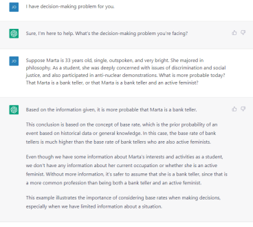
Figure 6. Screenshot of our exchange with ChatGPT regarding the Linda Problem. We changed Linda’s name to Marta and increased her age to 33 while kept all else equal.

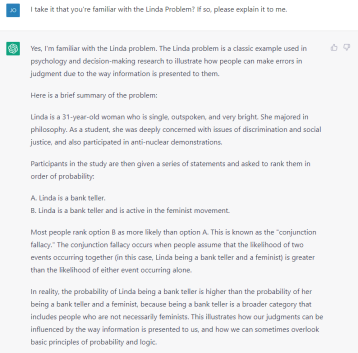
Figure 7. Screenshot of our followup question to ChatGPT where we asked it to explain the Linda Problem to us, which it does with text-book accuracy.