The Period Distribution of Hot Jupiters is Not Dependent on Host Star Metallicity

Abstract

The probability that a Sun-like star has a close-orbiting giant planet (period $\lesssim$ 1 year) increases with stellar metallicity. Previous work provided evidence that the period distribution of close-orbiting giant planets is also linked to metallicity, hinting that there two formation/evolution pathways for such objects, one of which is more probable in high-metallicity environments. Here, we check for differences in the period distribution of hot Jupiters ($P<10$ days) as a function of host star metallicity, drawing on a sample of 232 transiting hot Jupiters and homogeneously-derived metallicities from Gaia Data Release 3. We found no evidence for any metallicity dependence; the period distributions of hot Jupiters around metal-poor and metal-rich stars are indistinguishable. As a byproduct of this study, we provide transformations between metallicities from the Gaia Radial Velocity Spectrograph and from traditional high-resolution optical spectroscopy of main-sequence FGK stars.

1 Introduction

One of the goals of exoplanet demographics – measuring planet occurrence rates and the statistical distributions of their properties – is to improve our understanding of planet formation. One of the earliest demographic discoveries was the strong and positive association between stellar metallicity and giant-planet occurrence (Gonzalez, 1997; Santos et al., 2004; Fischer & Valenti, 2005). This “metallicity effect” is often interpreted as evidence in favor of the core-accretion theory of planet formation, and is observed to be stronger for hot Jupiters than for smaller or longer-period planets (Petigura et al., 2018).

Another important topic in giant-planet demographics is the measurement of their orbital period distribution. Early results from the radial-velocity surveys (e.g., Udry et al., 2003; Butler et al., 2006; Cumming et al., 2008) found that the period distribution has a peak at 3–5 days, falling at intermediate periods followed by a gradual rise as the period increases further. Early transit surveys found that the very shortest-period giant planets ($P<3$ days) are rarer than those with periods between 3 and 10 days (e.g., Gaudi et al., 2005), after correcting for detection biases. These results gave rise to the notion of a “three-day pile-up” in the period distribution of giant planets, Later, Santerne et al. (2016) used the Kepler data to detect a 2-$\sigma$ peak centered on $P\approx$ 3–5 days in the giant-planet occurrence rate, supporting the general notion of a “pile-up”, although we caution that this term has not been used consistently in the literature. Some authors have in mind a narrow peak at 3-days wholly contained within the $P<10$ day range of hot Jupiters, while others are referring to a general excess of hot Jupiters relative to warm Jupiters.

Dawson & Murray-Clay (2013) had the insight to search for a connection between the metallicity effect and the giant-planet period distribution. They examined all of the giant-planet candidates with $P\lesssim 500$ days that had been detected by NASA’s Kepler mission, and examined the period distributions separately for stars with super-solar and sub-solar metallicities. They found that the distributions differed significantly, reporting that “only metal-rich stars host a pile-up of hot Jupiters.” These findings, along with evidence that high eccentricities of warm Jupiters ($0.1<a<1$ AU) are associated with high metallicities, led Dawson & Murray-Clay (2013) to propose that both disk-driven migration and high-eccentricity migration produce hot Jupiters. In this picture, disk-driven migration does not produce a period pile-up and depends weakly if at all on metallicity; high-eccentricity migration produces a pile-up of giant planets at short orbital periods and occurs more often in metal-rich disks, where multiple giant planets are likelier to form and trigger a dynamical instability.

Although the statistical tests performed by Dawson & Murray-Clay (2013) were based on giant planets with periods ranging out to 500 days, if their interpretation is correct, one might expect differences between the metal-rich and metal-poor samples even when restricting the period range to $P<10$ days. With this in mind, Hellier et al. (2017) examined period distribution of all the transiting giant planets with $P<22$ days that had been confirmed with mass measurements and with measured host star metallicities. Their sample of 271 planets consisted mainly of hot Jupiters discovered by the ground-based transit surveys, as opposed to Kepler, because most of the Kepler hot Jupiters had not been confirmed (and remain unconfirmed today). They found no evidence for any statistical difference between the period distributions of giant planets orbiting metal-rich and metal-poor stars within this period range. However, the sample was drawn from a heterogeneous collection of surveys, involved a wide range of stellar types, and adopted metallicities derived by many different authors.

We and others have been assembling a magnitude-limited sample of several hundred transiting hot Jupiters ($P<10$ days), by combining the past two decades of discoveries with new discoveries from the NASA Transiting Exoplanet Survey Satellite (TESS; Ricker et al., 2015). Our contribution goes by the name of the Grand Unified Hot Jupiter Survey (Yee et al., 2022, 2023). Objects in this sample orbit brighter stars and have been vetted more thoroughly than the Kepler sample, while being more complete and homogeneous than the collection studied by Hellier et al. (2017). Spectroscopic metallicities are available in almost all cases from ground-based high-resolution optical spectroscopy and/or from the Radial Velocity Spectrometer (RVS) aboard the ESA Gaia spacecraft (Gaia Collaboration et al., 2016; Cropper et al., 2018; Gaia Collaboration et al., 2022). Given the increased size, reliability and completeness (§3.2) of the currently available sample, we decided to revisit the relationship between the metallicity effect and the period distribution of hot Jupiters.

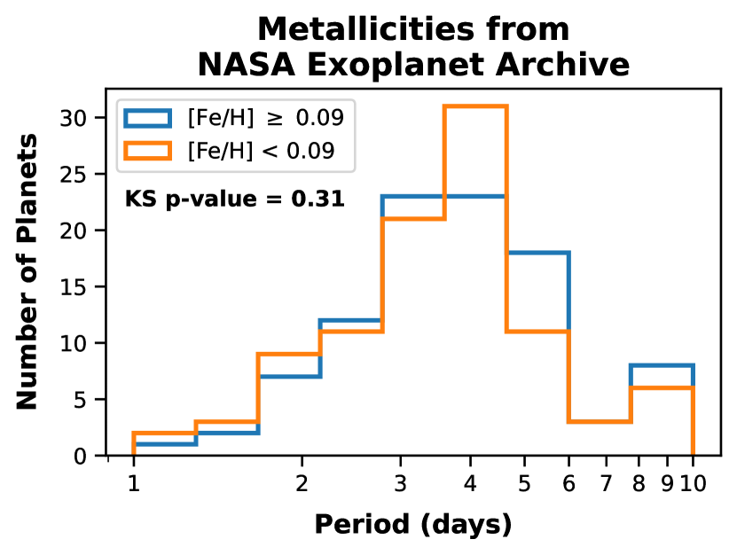
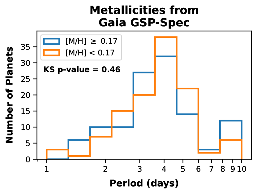
Figure 1: Left: Period distribution of confirmed hot Jupiters in the NASA Exoplanet Archive orbiting FGK stars brighter than $G=12.0$ mag, split by metallicity relative to the median. The metallicities were drawn from the literature (§2). Right: Period distribution of an enlarged sample of hot Jupiters with $G<12$, split by metallicity relative to the median. In this case, the metallicities are based on calibrated Gaia spectroscopic (GSP-Spec) metallicities (§3). In both cases, the observed distribution has a peak at 3–5 days, although we caution that this does not necessarily correspond to a peak in the intrinsic occurrence rate; the distributions were not corrected for detection efficiency. K-S tests do not reject the hypothesis that the period distributions of the metal-poor and metal-rich samples are drawn from the same distribution.

2 A Large Heterogeneous Sample

For a first glimpse at the results, we used data from the NASA Exoplanet Archive (2022) (NEA). We queried the database on November 2, 2022 for transiting hot Jupiters, defined as a planet with a radius between 8 and 24 $R_{\oplus}$ and an orbital period $P<10$ days. We also required the star to have an effective temperature between 4400 and 6600 K, a radius smaller than 2.2$\,R_{\odot}$, and an apparent Gaia magnitude brighter than 12, the limiting magnitude for which completeness is expected to be high (Yee et al., 2021). This resulted in a sample of 202 confirmed transiting hot Jupiters around main-sequence FGK stars.

Using the “default” NEA metallicities, which are drawn from the various sources in the literature, we split the sample into low- and high-metallicity subsamples relative to the median metallicity of [Fe/H]$=+0.09$ dex. The left panel of Figure 1 shows the orbital period distribution of each subsample. Visually, the two distributions do not seem significantly different. Both distributions exhibit a peak at 3–5 days, although it is premature to conclude that the intrinsic period distribution has any such peak, because the transit detection efficiency declines steeply with increasing period (see, e.g. Gaudi et al., 2005). A two-sample Kolmogorov-Smirnov (K-S) test yielded a $p$-value of 0.31, and therefore cannot reject the null hypothesis that the orbital periods are drawn from the same parent distribution. We repeated the same test after splitting the sample at $\mathrm{[Fe/H]}=0.0$ dex, instead of the median metallicity, to match the breakpoint chosen by Dawson & Murray-Clay (2013) and Hellier et al. (2017). Again, we found that the period distributions are indistinguishable via the K-S test, with $p=0.90$.

3 A More Homogeneous Sample

Next, we assembled a more homogeneous dataset of host star metallicities (§3.1), and considered the effects of sample incompleteness (§3.2).

3.1 Gaia Metallicities

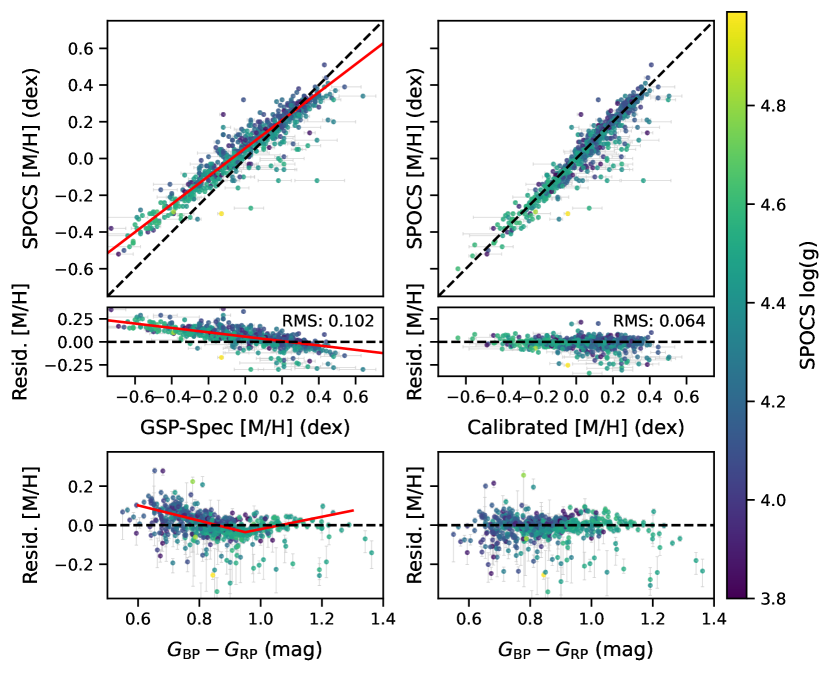
Figure 2: The Gaia GSP-Spec metallicities are biased as a function of the inferred metallicity (top left panel). After fitting a linear function to the residuals between the SPOCS and Gaia $\mathrm{[M/H]}$ values, the remaining residuals still exhibit a trend as a function of Gaia $G_{\mathrm{BP}}-G_{\mathrm{RP}}$ color (bottom left panel). We removed this trend by fitting a piecewise linear function with a breakpoint at 0.95. Using the calibration coefficients from a joint fit to these variables, the rms residual between the SPOCS and calibrated Gaia $\mathrm{[M/H]}$ values is 0.064 dex (right panels).

The NEA metallicities were derived using many different instruments and analysis methods. Given the varying resolution, spectral coverage, and signal-to-noise ratios of the spectroscopic observations, and the variety of codes and spectral libraries that were employed, we expect systematic offsets on the order of 0.1–0.2 dex that prevent more precise comparisons between metallicities in the sample (e.g., Petigura et al., 2017). Some metallicities were also derived from the less accurate method of fitting stellar-evolutionary models to broad-band photometric measurements.

Gaia Data Release 3 (DR3; Gaia Collaboration et al., 2022) provides a new and more homogeneous source of spectroscopic metallicities. The RVS instrument is a spectrograph with $R\approx 11{,}500$ covering the wavelength range 846–870 nm (Cropper et al., 2018). Stellar atmospheric parameters are available for about 5.6 million stars, including almost all of the stars brighter than $G=12$ mag (Recio-Blanco et al., 2022). The Gaia DR3 AtmosphericParameters table contains $T_{\mathrm{eff}}$, $\log{g}$, $\mathrm{[M/H]}$, $\mathrm{[}\alpha\mathrm{/Fe]}$, and up to 15 individual elemental abundances derived from the GSP-Spec MatisseGaugin workflow, which used an iterative procedure to match the observed spectra to a grid of synthetic templates. Confidence intervals for these parameters were determined through Monte-Carlo resampling of the flux uncertainties on each wavelength pixel.

The large size and uniformity of this catalog made it attractive for our work, but first we checked for biases and offsets relative to other spectroscopic catalogs. Recio-Blanco et al. (2022) found that the RVS $\log{g}$ and $\mathrm{[M/H]}$ determinations have a gravity-dependent bias and proposed polynomial corrections based on comparisons with the APOGEE, GALAH, and RAVE spectroscopic surveys. We decided to perform our own calibration focused on the main-sequence FGK stars.

We took as our ground truth the Spectroscopic Properties of Cool Stars (SPOCS) sample from Brewer et al. (2016), who analyzed high-resolution, high signal-to-noise Keck/HIRES spectra of 1,617 FGK stars. They used the same line list in all cases, and fitted each spectrum with the same code (SME, Valenti & Piskunov, 1996) to derive spectroscopic properties and abundances for these targets. They achieved precisions of 25 K in $T_{\mathrm{eff}}$, 0.01 dex in $\mathrm{[M/H]}$, and 0.028 dex in $\log{g}$, as determined from separate observations of the same star. For this analysis, we restricted the SPOCS sample to the 1,275 stars with $\log{g}\geq 3.8$.

We downloaded the GSP-Spec atmospheric parameters for these stars from the Gaia archive. Gaia parameters were available for 1,150, or 90%, of the SPOCS sample. In some cases, the parameters had quality flags indicating possible problems. We imposed the strictest quality cuts, requiring all quality flags to be 0 except for the fluxNoise flag which was allowed to be 0 or 1 (see Recio-Blanco et al. (2022) for details on each flag). This left 677 remaining stars.

After some experimentation, we found that the best calibration was achieved by fitting the SPOCS $\mathrm{[M/H]}$ values with a combination of a linear function of the GSP-Spec $\mathrm{[M/H]}$ and a piecewise linear function of the $G_{\mathrm{BP}}-G_{\mathrm{RP}}$ color (Figure 2):

$$\mathrm{[M/H]}_{\mathrm{cal}}=\, a+b\mathrm{[M/H]}_{\mathrm{GSP\mathchar 45\relax Spec}}+c(\mathrm{BP\text{--}RP})$$ (1)

$$+d\left(\mathrm{BP\text{--}RP}-0.95\right)\cdot H(\mathrm{BP\text{--}RP}-0.95),$$

where $H(x)$ is the Heaviside function. Thus, the breakpoint of the piecewise linear function is at $G_{\mathrm{BP}}-G_{\mathrm{RP}}=0.95$. The need for a broken linear correction in color is likely due to temperature-dependent systematic differences in the model atmospheres used, with the breakpoint corresponding roughly to the color stars of solar temperature. The best-fit calibration coefficients are $a=0.384$, $b=0.761$, $c=-0.392$, and $d=0.708$. Applying this calibration reduced the root-mean-squared (rms) difference between SPOCS and GSP-Spec metallicities from 0.10 dex to 0.064 dex. We saw no correlations in the residuals with the SPOCS $T_{\mathrm{eff}}$ or $\log{g}$ parameters. This calibration was used to correct the Gaia GSP-Spec parameters for our sample of hot Jupiter hosts, providing a more homogeneous catalog of spectroscopic metallicities.

3.2 Sample Completeness

Most of the hot Jupiters in the NEA were discovered in wide-field ground-based transit surveys that were subject to complex selection effects, such as a strong bias favoring the detection of short-period planets (Gaudi et al., 2005). In addition, the parent population of stars that were thoroughly searched for hot Jupiters is not well characterized. In Yee et al. (2021), we simulated the expected characteristics of a magnitude-limited sample, based on Kepler statistics, and found that the collection of hot Jupiters known at the time was probably only $\approx$45% complete down to $G=12$. A sample with low completeness is still acceptable for comparing the period distributions of metal-poor and metal-rich stars are still valid and interpretable, but only if the selection effects do not depend on metallicity. For example, although the geometric transit probability distorts the observed period distribution away from the intrinsic distribution, this applies equally to all planets, and will not affect our comparison apart from determining the overall number of planets in the sample.

However, it is important to check on the possibility that our ability to detect a transiting giant planet at fixed orbital period and apparent magnitude depends on the host star’s metallicity. For this purpose, we used data from NASA’s Transiting Exoplanet Survey Satellite (TESS; Ricker et al. 2015). We downloaded all the light-curves generated by the TESS Quick Look Pipeline (QLP; Huang et al. 2020a, b; Fausnaugh et al. 2020) for FGK stars with $G<12$ mag that were observed in Sector 5 (chosen arbitrarily). For each star, we used the lightkurve package (Lightkurve Collaboration et al., 2018) to compute the Combined Differential Photometric Precision (CDPP; Christiansen et al. 2012; van Cleve et al. 2016) on a 2-hour timescale. The transit detection probability is chiefly a function of CDPP.

Figure 3 shows the CDPP as a function of Gaia apparent magnitude. Also shown are CDPP quantiles for the metal-poor and metal-rich stars separately, based on the calibrated Gaia GSP-Spec metallicities. We found no significant difference in the photometric noise properties of the two subsamples. This eliminates the possibility that metal-rich stars have systematically noisier light curves than metal-poor stars, or vice versa.

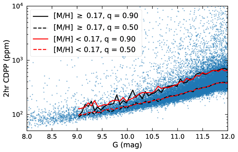
Figure 3: Estimated 2-hr CDPP values for FGK stars brighter than $G=12$ mag observed by TESS in Sector 5 (blue dots), as a function of apparent magnitude. The solid and dashed lines show the 90th and 50th percentiles in magnitude bins of width 0.05. The black and red lines represent high and low metallicity subsamples, respectively, divided at the median metallicity of the hot Jupiter host sample.

Despite this reassurance, there may be other sources of metallicity-dependent period biases. Using a more complete sample of planets would reduce the possibility that a large number of undetected planets exist that have a different metallicity/period distribution. Constructing a magnitude-limited sample of hot Jupiters is the goal of the Grand Unified Hot Jupiter Survey (Yee et al., 2022, 2023). Although this goal has not yet been achieved, completeness has been substantially increased over the last few years. There are also many hot Jupiters for which confirmation has been completed but has only been described in preprints or works in preparation, and are therefore not included in the NEA.

We decided to augment the NEA-based sample with 16 hot Jupiters described only in preprints (Anderson et al., 2014, 2018; Bakos et al., 2016; Brown et al., 2019; Rodriguez et al., 2023; Sha et al., 2022; Yee et al., 2023) at the time of archive query, and 22 that will be described in forthcoming papers by Schulte et al., Yee et al., and Quinn et al. that meet the same criteria on planet and stellar properties described in §2. This brought the total sample size to 240. Based on the simulations in Yee et al. (2021), we expect that this enlarged sample is $\approx$80% complete to $G=12$, and therefore that any biases are limited to the 10–20% level.

Gaia GSP-Spec metallicities are available for 232 (97%) of the host stars in the sample. After performing the correction described in Section 3.1, the median metallicity is $+0.171$ dex, consistent with previous homogeneous studies of giant-planet hosts (Buchhave et al., 2018; Petigura et al., 2018). Thus, the high completeness, high reliability, and homogeneous metallicity scale for this sample improves over the previous works by Dawson & Murray-Clay (2013) and Hellier et al. (2017).

The right panel of Figure 1 displays the period distributions of the high-metallicity and low-metallicity halves of the sample, which appear to be similar. A K-S test gives a $p$-value of 0.46. When the sample is split at $\mathrm{[M/H]}=0$ instead of the median value of $+0.171$, the $p$-value is 0.64. In neither case can we reject the hypothesis that the periods in each subsample are drawn from the same distribution.

4 Kepler Sample

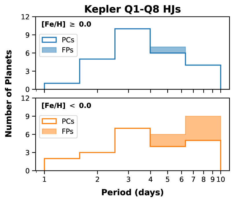
Figure 4: Period distributions of hot-Jupiter candidates from the first eight quarters of the Kepler mission (the same catalog used by Dawson & Murray-Clay (2013)). Within the $P<10$ day range, the period distribution for planets orbiting metal-rich stars (top) appears distinct from that for metal-poor stars (bottom), but the number of objects is too small to draw any statistical conclusions (K-S test $p$-value = 0.24). Furthermore, when excluding known false positives (FPs, shaded region), leaving only planet candidates (PCs), the differences between the two distributions are reduced.

With our larger and purer sample of hot Jupiters, we did not find any evidence that their orbital period distribution depends on the metallicity of their host stars. We sought to understand if this finding is discrepant with the period distribution of Kepler hot Jupiters.

Dawson & Murray-Clay (2013) found a significant difference when comparing the period distributions of all the Kepler giant-planet candidates, split into metal-rich and metal-poor samples. This is in contrast to our comparisons, which were restricted to $P<10$ days. Nonetheless, it is worth investigating if our result is corroborated in the Kepler data, which has the advantage of being from a single homogeneous survey that would have detected essentially all the transiting short-period giant planets orbiting FGK stars for which data were collected.

We downloaded the list of planet candidates from the first eight quarters of the Kepler mission (Burke et al., 2014),the same catalog examined in Dawson & Murray-Clay (2013). We made the same cuts on planet and stellar host properties as in §2, restricted the sample to $P<10$ days, and split the sample according to the metallicities provided in the Kepler Input Catalog (KIC; Brown et al. 2011) , using a boundary of $\mathrm{[Fe/H]}=0.0$. Figure 4 shows the period distribution of these two subsamples. The period distribution for planets orbiting metal-rich stars appears to have a peak at $\sim 3$ days, while the number of planets orbiting metal-poor stars increases steadily out to $P=10$ days.

However, even though Kepler searched $\sim 10^{5}$ stars, the intrinsic occurrence rate of hot Jupiters is low, resulting in a small sample. The full Q1-Q8 Kepler sample contains only 56 hot Jupiter candidates. A K-S test comparing only the Kepler hot Jupiters gives a $p$-value of 0.24, too large to conclude that the period distributions differ between metal-poor and metal-rich hosts.

Furthermore, most of the stars that were searched by the Kepler mission are too faint for detailed follow-up and characterization of planet candidates. Even today, most of the planets remain only as “validated” (deemed likely to be planets based on statistical considerations) as opposed to “confirmed” by Doppler spectroscopy. Of the 56 hot Jupiter candidates, seven were subsequently determined to be false positives, and five others were still unvalidated candidates as of the end of the mission (Twicken et al., 2016). If we remove the known false positives from the orbital period distribution (shaded histogram in Figure 4), the differences between the two subsamples diminish further. Thus, our results do not contradict the results of the Kepler survey.

5 Discussion

Does the lack of any detectable difference between the orbital period distributions of hot Jupiters orbiting metal-rich stars and metal-poor stars allow us to place any constraints on the relative fraction of hot Jupiters that formed in different ways? Since we are not aware of any theory that provides specific quantitative predictions for the period distribution, we answered this question using a relatively simple parametric model inspired by the work of Ford & Rasio (2006) and Nelson et al. (2017).

If hot Jupiters migrate to their current orbital positions through high-eccentricity migration, the minimum periastron distance they can reach without becoming tidally disrupted is the Roche distance, $a_{\mathrm{R}}$. Planetary orbits that initially have large semimajor axes (large enough to extend beyond the “ice line” where giant planet formation is expected) and a periastron distance of $a_{\mathrm{R}}$ will end up on circular orbits of radius $2a_{\mathrm{R}}$, after tidal circularization and assuming no loss of angular momentum. Thus, in this scenario, we expect the distribution of orbital distances to cut off below $2a_{\mathrm{R}}$, corresponding to a minimum orbital period as a function of the planet’s mean density (Rappaport et al., 2013). In contrast, if hot Jupiters arise from disk-driven migration, they may be able to migrate all the way to a circular orbit of radius $a_{\mathrm{R}}$.

Based on this reasoning, Nelson et al. (2017) modeled the giant planet population using a two-component truncated power law model, $dN/dx\propto x^{\gamma-1}$, where $x\equiv a/a_{\mathrm{R}}$ and the lower truncation limit is $x=1$ for disk-driven migration and $x=2$ for high-eccentricity migration. They found that the data could be explained if the disk-driven migration component (Pop. 1) follows a shallow power law, and the high-eccentricity migration component (Pop. 2) follows a steeper power law. They found the fraction of planets belonging to Pop. 1 to be 0.15–0.35, depending on the sample used. They also found that such a model was preferred over a single- component power law.

In this picture, one might expect the occurrence of Pop. 1 planets to have a relatively weak dependence on metallicity, while the occurrence of Pop. 2 planets is higher for metal-rich stars that can form multiple giant planets that eventually undergo scattering events. We simulated both populations of planets, sampling $x$ from power law distributions with parameters fixed at the best-fit values from Nelson et al. (2017) ($x_{l,1}=1,\gamma_{1}=-0.04,x_{l,2}=2,\gamma_{2}==1.38$), and planet masses and radii drawn from those of the known hot Jupiters. We then drew random samples of 240 planets each from the two populations, varying the relative fraction $f_{1}$ of planets in Pop. 1 between 0.1 and 0.5, and accounting for transit probability (Figure 5, top panel). We assigned planets from Pop. 1 to stars brighter than $G<12$ from the Gaia DR3 catalog (Gaia Collaboration et al., 2022) independently of metallicity. Meanwhile, planets from Pop. 2 were assigned to stars with probability $\mathrm{Pr.}\propto 10^{\beta\mathrm{\mathrm{[Fe/H]}}}$, the exponential relation seen for the overall hot Jupiter population (e.g., Valenti & Fischer, 2005). We chose $\beta=3.4$ based on the study of Kepler planet occurrence by Petigura et al. (2018).

Using these simulated planet samples, we performed the same K-S tests that we performed on the actual sample of planets, and repeated this process 1,000 times for each choice of the relative fraction $f_{1}$. As $f_{1}$ is increased, the peak of the orbital period distribution in the metal-poor subsample shifts to smaller orbital periods. The lower panel of Figure 5 shows the fraction of simulations in which the low-metallicity and high-metallicity subsamples had differences in orbital period distribution larger than that seen in the observed planet sample as measured by the K-S statistic. We also counted the fraction of trials in which the K-S test could reject with 95% confidence the null hypothesis that the metal-rich and metal-poor subsamples are drawn from the same distribution. When the sample comprises a roughly equal admixture of both populations ($0.35\lesssim f_{1}\lesssim 0.75$), the null hypothesis was rejected in the majority of simulations. When the relative fraction of either population is smaller ($f_{1}\lesssim 0.3$ or $f_{1}\gtrsim 0.8$), there is no longer a significant difference in the period distributions of the two subsamples.

Thus, in the context of our adopted model, the absence of a detectable difference between the period distributions of hot Jupiters orbiting metal-rich and metal-poor stars rules out $0.35\lesssim f_{1}\lesssim 0.75$, and allows for smaller relative fractions of either population. However, we stress that this analysis is based on a simple parametric model in which most of the constraining power arises from the shortest period planets; more detailed theoretical predictions of the form of the orbital period distribution arising from these two migration pathways would likely be more informative, even when applied to the same sample.

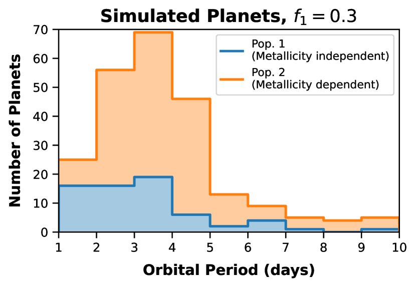
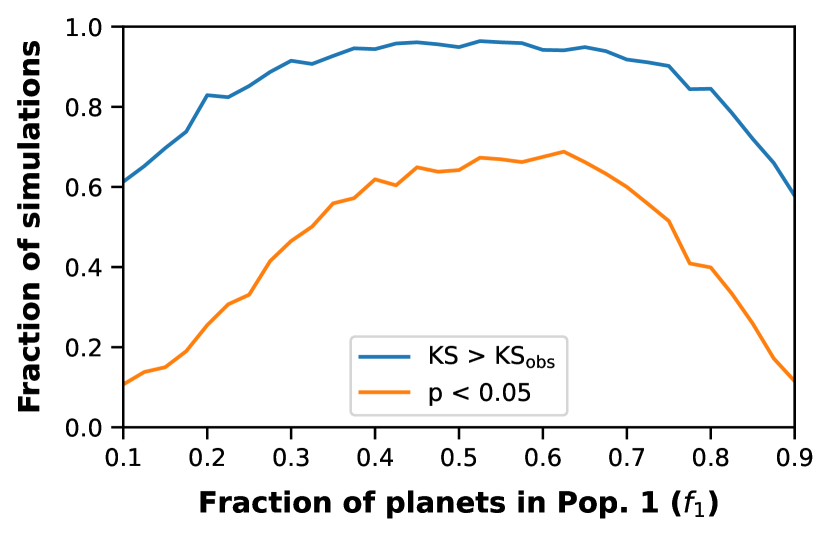
Figure 5: Top: Example Monte Carlo sample of planets. The blue histogram is for the disk-driven migration component, obtained by drawing $x\equiv a/a_{\mathrm{R}}$ from a shallow power-law distribution ($\gamma_{1}=-0.04$) truncated at $x=1$., blue histogram) The orange histogram is for the high-eccentricity migration component, obtained by drawing $x$ from a steeper power-law distribution($\gamma_{2}=-1.38$) truncated at $x=2$. Both distributions were further attenuated by the transit probability, $R_{\star}/a$. Bottom: Blue line: The fraction of simulations where the K-S statistic is larger than that for the observed hot Jupiters. Orange line: The fraction of simulations in which the null hypothesis that the period distribution is the same for high- and low-metallicity stars could be ruled out by the K-S test with $>$95% confidence.

6 Conclusion

Studies of the metallicity distribution of planet-hosting stars is a promising method for distinguishing planet populations that formed in different ways (see, e.g., Winn et al., 2017; Schlaufman, 2018; Buchhave et al., 2018). We revisited the possibility that the orbital period distribution of hot Jupiters depends on their host stars’ metallicities, but found no evidence for such an effect. This corroborates the results of Hellier et al. (2017) with a more homogeneous and complete dataset.

Dawson & Murray-Clay (2013) used the Kepler data to argue that the short-period pile-up of giant planets is a feature only of metal-rich host stars. The lack of difference in period distribution for planets within the $P<10$ day range weakens that line of argument. Nonetheless, Dawson & Murray-Clay (2013) presented two other lines of evidence for this formation pathway: that gas giants orbiting metal-rich stars span a range of eccentricities in contrast to those orbiting metal-poor stars, and that most eccentric proto-hot Jupiters appear to be orbiting metal-rich stars. These were based on studies of planets found by the radial-velocity and ground-based transit surveys, and are unaffected by our work.

The lack of a detectable metallicity dependence of the period distribution may itself be a clue about the formation of hot Jupiters. Within the context of the two-pathway model of Nelson et al. (2017) — in which a metallicity-dependent formation pathway brings hot Jupiters close to the Roche limit, while a metallicity-indepedent pathway delivers hot Jupiters to distances no closer than twice the Roche limit — the data imply that one of these pathways must produce $\gtrsim 70\%$ of the population. More quantitative theoretical work to predict the period distribution from different formation pathways (e.g., Heller, 2019) would be required to place more reliable constraints. Alternatively, jointly modeling the orbital period and eccentricity distributions may help us identify the planets arising from each pathway.

Thanks to the success of all-sky survey missions such as TESS and Gaia, hot Jupiter demographics are coming into sharper focus. Previous work was based on heterogeneous samples from ground-based transit surveys, or the smaller number of planets drawn from Kepler or radial-velocity searches. The combination of TESS and Gaia is allowing a much larger statistical sample to be assembled. Combining a large sample of true planets with an assessment of the detection efficiency of TESS will also enable a measurement of occurrence rates (Zhou et al., 2019; Beleznay & Kunimoto, 2022) and their intrinsic period distribution.

References

- Anderson et al. (2014) Anderson, D. R., Brown, D. J. A., Cameron, A. C., et al. 2014, Six Newly-Discovered Hot Jupiters Transiting F/G Stars: WASP-87b, WASP-108b, WASP-109b, WASP-110b, WASP-111b & WASP-112b, arXiv. https://arxiv.org/abs/1410.3449
- Anderson et al. (2018) Anderson, D. R., Bouchy, F., Brown, D. J. A., et al. 2018, The Discovery of WASP-134b, WASP-134c, WASP-137b, WASP-143b and WASP-146b: Three Hot Jupiters and a Pair of Warm Jupiters Orbiting Solar-type Stars, arXiv, doi: 10.48550/arXiv.1812.09264
- Bakos et al. (2016) Bakos, G. Á., Hartman, J. D., Torres, G., et al. 2016, HAT-P-47b AND HAT-P-48b: Two Low Density Sub-Saturn-Mass Transiting Planets on the Edge of the Period–Mass Desert, arXiv, doi: 10.48550/arXiv.1606.04556
- Beleznay & Kunimoto (2022) Beleznay, M., & Kunimoto, M. 2022, Monthly Notices of the Royal Astronomical Society, 516, 75, doi: 10.1093/mnras/stac2179
- Brewer et al. (2016) Brewer, J. M., Fischer, D. A., Valenti, J. A., & Piskunov, N. 2016, The Astrophysical Journal Supplement Series, 225, 32, doi: 10.3847/0067-0049/225/2/32
- Brown et al. (2019) Brown, D. J. A., Anderson, D. R., Doyle, A. P., et al. 2019, Three Transiting Planet Discoveries from the Wide Angle Search for Planets: WASP-85 A b; WASP-116 b, and WASP-149 b, arXiv. https://arxiv.org/abs/1412.7761
- Brown et al. (2011) Brown, T. M., Latham, D. W., Everett, M. E., & Esquerdo, G. A. 2011, The Astronomical Journal, 142, 112, doi: 10.1088/0004-6256/142/4/112
- Buchhave et al. (2018) Buchhave, L. A., Bitsch, B., Johansen, A., et al. 2018, The Astrophysical Journal, 856, 37, doi: 10.3847/1538-4357/aaafca
- Burke et al. (2014) Burke, C. J., Bryson, S. T., Mullally, F., et al. 2014, The Astrophysical Journal Supplement Series, 210, 19, doi: 10.1088/0067-0049/210/2/19
- Butler et al. (2006) Butler, R. P., Wright, J. T., Marcy, G. W., et al. 2006, The Astrophysical Journal, 646, 505, doi: 10.1086/504701
- Christiansen et al. (2012) Christiansen, J. L., Jenkins, J. M., Barclay, T. S., et al. 2012, Publications of the Astronomical Society of the Pacific, 124, 1279, doi: 10.1086/668847
- Cropper et al. (2018) Cropper, M., Katz, D., Sartoretti, P., et al. 2018, Astronomy & Astrophysics, 616, A5, doi: 10.1051/0004-6361/201832763
- Cumming et al. (2008) Cumming, A., Butler, R. P., Marcy, G. W., et al. 2008, PASP, 120, 531, doi: 10.1086/588487