HyHTM: Hyperbolic Geometry based
Hierarchical Topic Models

Abstract

Hierarchical Topic Models (HTMs) are useful for discovering topic hierarchies in a collection of documents. However, traditional HTMs often produce hierarchies where lower-level topics are unrelated and not specific enough to their higher-level topics. Additionally, these methods can be computationally expensive. We present HyHTM - a Hyperbolic geometry based Hierarchical Topic Models - that addresses these limitations by incorporating hierarchical information from hyperbolic geometry to explicitly model hierarchies in topic models. Experimental results with four baselines show that HyHTM can better attend to parent-child relationships among topics. HyHTM produces coherent topic hierarchies that specialise in granularity from generic higher-level topics to specific lower-level topics. Further, our model is significantly faster and leaves a much smaller memory footprint than our best-performing baseline.We have made the source code for our algorithm publicly accessible.

1 Introduction

The topic model family of techniques is designed to solve the problem of discovering human-understandable topics from unstructured corpora paul2014discovering where a topic can be interpreted as a probability distribution over words blei2003latent. Hierarchical Topic Models (HTMs), in addition, organize the discovered topics in a hierarchy, allowing them to be compared with each other. The topics at higher levels are generic and broad while the topics lower down in the hierarchy are more specific teh2004sharing.

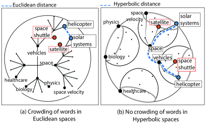
Figure 1: In figure (a) we see a concept tree in Euclidean spaces. Words such as space shuttle and satellite, which belong to moderately different super-concepts such as vehicles and space, respectively, are brought closer together due to their semantic similarity. This leads to a convergence of their surrounding words, such as helicopter and solar system, creating a false distance relationship and a crowding effect in Euclidean spaces. In figure (b), we see a concept tree in Hyperbolic spaces (Poincaré ball), which inherently has more space (represented by grey circles) than Euclidean spaces. The distances here grow exponentially towards the edge of the ball, and the concepts at deeper levels such as helicopter and solar systems move apart in these growing spaces and are far from each other. The dashed blue line shows how the distances in both spaces are calculated.

While significant efforts have been made to develop HTMs blei2003hierarchical; chirkova2016additive; isonuma2020tree; viegas2020cluhtm, there are still certain areas of improvement. First, the ordering of topics generated by these approaches provides little to no information about the granularity of concepts within the corpus. By granularity, we mean that topics near the root should be more generic, while topics near the leaves should be more specific. Second, the lower-level topics must be related to the corresponding higher-level topics. Finally, some of these approaches such as CluHTM viegas2020cluhtm are very computationally intensive. We argue that these HTMs have such shortcomings primarily because they do not explicitly account for the hierarchy of words between topics.

Most of the existing approaches use document representations that employ word embeddings from euclidean spaces. These spaces tend to suffer from the crowding problem which is the tendency to accommodate moderately distant words close to each other van2008visualizing. There are several notable efforts that have shown that Euclidean spaces are suboptimal for embedding concepts in hierarchies such as trees, words, or graph entities chami2019hyperbolic; chami2020low; guo2022co. In figure 1(a), we show the crowding of concepts in euclidean spaces. Words such as space shuttle and satellite, which belong to moderately different concepts such as vehicles and space, respectively, are brought closer together due to their semantic similarity. This also leads to a convergence of their surrounding words, such as helicopter and solar system creating a false distance relationship. As a result of this crowding, topic models such as CluHTM that use Euclidean word similarities in their formulation tend to mix words that belong to different topics.

Contrary to this, hyperbolic spaces are naturally equipped to embed hierarchies with arbitrarily low distortion nickel2017poincare; tifrea2018poincar; chami2020low. The way distances are computed in these spaces are similar to tree distances, i.e., children and their parents are close to each other, but leaf nodes in completely different branches of the tree are very far apart chami2019hyperbolic. In figure 1(b), we visualise this intuition on a Poincaré ball representation of hyperbolic geometry (discussed in detail in Section 3). As a result of this tree-like distance computation, hyperbolic spaces do not suffer from the crowding effect and words like helicopter and satellite are far apart in the embedding space.

Inspired by the above intuition and to tackle the shortcomings of traditional HTMs, we present HyHTM, a Hyperbolic geometry based Hierarchical Topic Model which uses hyperbolic geometry to create topic hierarchies that better capture hierarchical relationships in real-world concepts. To achieve this, we propose a novel method of incorporating semantic hierarchy among words from hyperbolic spaces and encoding it explicitly into topic models. This encourages the topic model to attend to parent-child relationships between topics.

Experimental results and qualitative examples show that incorporating hierarchical information guides the lower-level topics and produces coherent, specialised, and diverse topic hierarchies (Section LABEL:sect:experiments). Further, we conduct ablation studies with different variants of our model to highlight the importance of using hyperbolic embeddings for representing documents and guiding topic hierarchies (Section LABEL:sect:roleofHyperbolic). We also compare the scalability of our model with different sizes of datasets and find that our model is significantly faster and leaves much smaller memory footprint than our best-performing baseline (Section LABEL:sect:speed). We also present qualitative results in Section LABEL:sect:quality), where we observe that HyHTM topic hierarchies are much more related, diverse and specialised. Finally, we discuss and perform in-depth ablations to show the role of hyperbolic spaces and importance of every choice we made in our algorithm (See Section LABEL:sect:roleofHyperbolic).

Figure 2: Comparing our Hyperbolic-based HyHTM model to the Euclidean-based CluHTM, for selected 20News document labels (comp.graphics, comp.os.ms-windows.misc), we find that HyHTM is better at discriminating between similar document labels. CluHTM’s root-level topics are not related to computer concepts, and it cannot separate these labels at lower levels. HyHTM groups them in the same root level and separates them into different lower-level topics, showing the advantage of using hyperbolic embeddings over euclidean ones to avoid the crowding problem. We show the top words with the highest probability for the topics.

2 Related Work

To the best of our knowledge, HTMs can be classified into three categories, (I) Bayesian generative model like hLDA blei2003hierarchical, and its variants paisley2013nested; kim2012modeling; tekumalla2015nested utilize bayesian methods like Gibbs sampler for inferring latent topic hierarchy. These are not scalable due to the high computational requirements of posterior inference. (II) Neural topic models like TSNTM isonuma2020tree and others wang2021layer; pham2021neural use neural variational inference for faster parameter inference and some heuristics to learn topic hierarchies but lack the ability to learn appropriate semantic embeddings for topics. Along with these methods, there are (III) Non-negative matrix factorization (NMF) based topic models, which decompose a term-document matrix (like bag-of-words) into low-rank factor matrices to find latent topics. The hierarchy is learned using some heuristics HSOC; liu2018topic or regularisation methods chirkova2016additive based on topics in the previous level.

However, the sparsity of the BoW representation for all these categories leads to incoherent topics, especially for short texts. To overcome this, some approaches have resorted to incorporating external knowledge from knowledge bases (KBs) duan2021topicnet; wang2022knowledge or leveraging word embeddings meng2020hierarchical. Pre-trained word embeddings are trained on a large corpus of text data and capture the relationships between words such as semantic similarities, and concept hierarchies. These are used to guide the topic hierarchy learning process by providing a semantic structure to the topics. viegas2020cluhtm utilizes euclidean embeddings for learning the topic hierarchy. However, tifrea2018poincar; nickel2017poincare; chami2020low; dai2020apo have shown how the crowding problem in Euclidean spaces makes such spaces suboptimal for representing word hierarchies. These works show how Hyperbolic spaces can model more complex relationships better while preserving structural properties like concept hierarchy between words. Recently, shihyperminer made an attempt to learn topics in hyperbolic embedding spaces. Contrary to the HTMs above, this approach adopts a bottom-up training where it learns topics at each layer individually starting from the bottom, and then during training leverages a topic-linking approach from duan2021sawtooth, to link topics across levels. They also have a supervised variant that incorporates concept hierarchy from KBs.

Our approach uses latent word hierarchies from pretrained hyperbolic embeddings to learn the hierarchy of topics that are related, diverse, specialized, and coherent.

3 Preliminaries

We will first review the basics of Hyperbolic Geometry and define the terms used in the remainder of this section. We will then describe the basic building blocks for our proposed solution, followed by a detailed description of the underlying algorithm.

3.1 Hyperbolic Geometry

Hyperbolic geometry is a non-Euclidean geometry with a constant negative Gaussian curvature. Hyperbolic geometry does not satisfy the parallel postulate of Euclidean geometry. Consequently, given a line and a point not on it, there are at least two lines parallel to it. There are many models of hyperbolic geometry, and we direct the interested reader to an excellent exposition of the topic by book-hyperbolic. We base our approach on the Poincaré ball model, where all the points in the geometry are embedded inside an $n$-dimensional unit ball equipped with a metric tensor (nickel2017poincare). Unlike Euclidean geometry, where the distance between two points is defined as the length of the line segment connecting the two points, given two points $u\in\mathbb{D}^{n}$ and $v\in\mathbb{D}^{n}$, the distance between them in the Poincaré model is defined as follows:

$$\begin{multlined}d_{P}(u,v)=\operatorname{arcosh}\left(1+2\frac{{\|u-v\|}^{2}}{(1-\|u\|^{2})(1-\|v\|^{2})}\right)\end{multlined}d_{P}(u,v)=\operatorname{arcosh}\left(1+2\frac{{\|u-v\|}^{2}}{(1-\|u\|^{2})(1-\|v\|^{2})}\right)$$ (1)

Here, $\operatorname{arcosh}$ is the inverse hyperbolic cosine function, and $\|.\|$ is the Euclidean norm. Figure 1 has shown an exemplary visualization of how words get embedded in hyperbolic spaces using the Poincaré ball model. As illustrated in Figure 1(b), distances in hyperbolic space follow a tree-like path, and hence they are informally also referred to as tree distances. As can be observed from the figure, the distances grow exponentially larger as we move toward the boundary of the Poincaré ball. This alleviates the crowding problem typical to Euclidean spaces, making hyperbolic spaces a natural choice for the hierarchical representation of data.

3.2 Matrix Factorization for Topic Models

A topic can be defined as a ranked list of strongly associated terms representative of the documents belonging to that topic. Let us consider a document corpus $\mathcal{D}$ consisting of $n$ documents $d_{1},d_{2},\dots,d_{n}$, and let $\mathcal{V}$ be the corpus vocabulary consisting of $m$ distinct words $w_{1},w_{2},\dots,w_{m}$. The corpus can also be represented by a document-term matrix $\textbf{A}\in\mathbb{R}^{n\times m}$ such that $\textbf{A}_{ij}$ represents the relative importance of word $w_{j}$ in document $d_{i}$ (typically represented by the TF-IDF weights of $w_{i}$ in $d_{j}$).

A popular way of inferring topics from a given corpus is to factorize the document-term matrix. Typically, non-negative Matrix Factorization (NMF) is employed to decompose the document-term matrix, A, into two non-negative approximate factors: $\textbf{W}\in\mathbb{R}^{n\times\textbf{N}}$ and $\textbf{H}\in\mathbb{R}^{\textbf{N}\times m}$. Here, N can be interpreted as the number of underlying topics. The factor matrix W can then be interpreted as the document-topic matrix, providing the topic memberships for documents, and H, the topic-term matrix, describes the probability of a term belonging to a given topic. This basic algorithm can also be applied recursively to obtain a hierarchy of topics by performing NMF on the set of documents belonging to each topic produced at a given level to get more fine-grained topics (chirkova2016additive; viegas2020cluhtm).

4 Hierarchical Topic Models Using Hyperbolic Geometry

We now describe HyHTM – our proposed Hyperbolic geometry-based Hierarchical Topic Model. We first describe how we capture semantic similarity and hierarchical relationships between terms in hyperbolic space. We then describe the step-by-step algorithm for utilizing this information to generate a topic hierarchy.

4.1 Learning Document Representations in Hyperbolic Space and Root Level Topics

As discussed in Section 3.2, the first step in inferring topics from a corpus using NMF is to compute the document-term matrix A. A typical way to compute the document-term matrix A is by using the TF-IDF weights of terms in a document that provides reprsentations of the documents in the term space. However, usage of TF-IDF (and its variants) results in sparse representations and ignores the semantic relations between different terms by considering only the terms explicitly present in a given document. viegas2019cluwords proposed an alternative formulation for document representations that utilizes pre-trained word embeddings to enrich the document representations by incorporating weights for words that are semantically similar to the words already present in the document. The resulting document representations are computed as follows.

$$\textbf{A}=(\textbf{TF}\times\textbf{M}_{\text{S}})\odot(\mathbf{1}\times\textbf{IDF}^{T})$$ (2)

Here, $\odot$ indicates the Hadamard product. A is the $n\times m$ document-term matrix. TF is the term-frequency matrix such that $\textbf{TF}_{i,j}=tf(d_{i},w_{j})$ and $\textbf{M}_{\text{S}}$ is the $m\times m$ term-term similarity matrix that captures the pairwise semantic relatedness between the terms and is defined as $\textbf{M}_{\text{s}_{i,j}}=sim(w_{i},w_{j})$, where $sim(w_{i},w_{j})$ represents the similarity between terms $w_{i}$ and $w_{j}$ and can be computed using typical word representations such as word2vec (w2v) and GloVe (pennington2014glove). Finally, IDF is the $m\times 1$ inverse-document-frequency vector representing the corpus-level importance of each term in the vocabulary. Note that viegas2019cluwords used the following modified variant of IDF in their formulation, which we also chose in this work.

$$\textbf{IDF}(i)=\log\left(\frac{|D|}{\sum_{d\in D}\mu\left(w_{i},d\right)}\right)$$ (3)

Here, $\mu\left(w_{i},d\right)$ is the average of the similarities between term $w_{i}$ and all the terms $w$ in document $d$ such that $\textbf{M}_{\text{S}}(w_{i},w)\neq 0$. Thus, unlike traditional IDF formulation where the denominator is document-frequency of a term, the denominator in the above formulation captures the semantic contribution of $w_{i}$ to all the documents.

In our work, we adapt the above formulation to obtain document representations in Hyperbolic spaces by using Poincaré GloVe embeddings (tifrea2018poincar), an extension of the traditional Euclidean space GloVe (pennington2014glove) to hyperbolic spaces. Due to the nature of the Poincaré Ball model, the resulting embeddings in the hyperbolic space arrange the correspondings words in a hierarchy such that the sub-concept words are closer to their parent words than the sub-concept words of other parents.

There is one final missing piece of the puzzle before we can obtain suitable document representations in hyperbolic space. Recall that due to the nature of the Poincaré Ball model, despite all the points being embedded in a unit ball, the hyperbolic distances between points, i.e., tree distances (Section 3.1) grow exponentially as we move towards boundary of the ball (see Figure 1). Consequently, the distances are bounded between $0$ and $1$. As NMF requires all terms in the input matrix to be positive, we cannot directly use these distances to compute the term-term similarity matrix $\textbf{M}_{\text{S}}$ in Equation (2) as $1-d_{P}\left(w,w^{\prime}\right)$ can be negative. To overcome this limitation, we introduce the notion of Poincaré Neighborhood Similarity, ($s_{p_{n}}$), which uses a neighborhood normalization technique. The $k$-neighborhood of a term $w$ is defined as the set of top k-nearest terms ${w_{1},...,w_{k}}$ in the hyperbolic space and is denoted as $n_{k}(w)$. For every term in the vocabulary $\mathcal{V}$, we first calculate the pair-wise poincaré distances with other terms using Equation (1). Then, for every term $w\in\mathcal{V}$, we compute similarity scores with all the other terms in its $k$-neighborhood $n_{k}(w)$ by dividing each pair-wise poincaré distance between the term and its neighbor by the maximum pair-wise distance in the neighborhood. This can be represented by the following equation where $w^{\prime}\in n_{k}(w)$:

$$s_{p_{n}}\left(w,w^{\prime}\right)=1-\frac{d_{P}\left(w,w^{\prime}\right)}{\max\limits_{w_{a},w_{b}\in n_{k}(w)}(d_{P}\left(w_{a},w_{b}\right))}$$ (4)

With this, we can now compute the term-term similarity matrix $\bm{M_{S}}$ as follows.

$$\textbf{M}_{\text{S}}{(w,w^{\prime})}=\begin{cases}s_{p_{n}}\left(w,w^{\prime}\right)&\text{ if }s_{p_{n}}\left(w,w^{\prime}\right)\geq\alpha,\\ 0&\text{ otherwise }\end{cases}$$ (5)

Note that there are two hyperparameters to control the neighborhood – (i) the neighborhood size using $k_{s}$; and (ii) the quality of words using $\alpha$, which keeps weights only for the pair of terms where the similarity crosses the pre-defined threshold $\alpha$ thereby reducing noise in the matrix. Without $\alpha$, words with very low similarity may get included in the neighborhood eventually leading to noisy topics.

We now have all the ingredients to compute the document-representation matrix A in the hyperbolic space and NMF can be performed to obtain the first set of topics from the corpus as described in Section 3.2. This gives us the root level topics of our hierarchy. Next, we describe how we can discover topics at subsequent levels.

4.2 Building the Topic Hierarchy

In order to build the topic hierarchy, we can iteratively apply NMF for topics discovered at each level as is typically done in most of the NMF based approaches. However, do note that working in the Hyperbolic space allows us to utilize hierarchical information encoded in the space to better guide the discovery of topic hierarchies. Observe that the notion of similarity in the hyperbolic space as defined in Equation(4) relies on the size of the neighborhood. In large neighborhood, a particular term will include not only its immediate children and ancestors but also other semantically similar words that may not be hierarchically related. On the other hand, a small neighborhood will include only the immediate parent-child relationships between the words, since subconcept words are close to their concept words. HyHTM uses this arrangement of words in hyperbolic space to explicitly guide the lower-level topics to be more related and specific to higher-level topics. In order to achieve this, we construct a Term-Term Hierarchy matrix, $\textbf{M}_{\text{H}}\in R^{|V|\times|V|}$ as follows.

$$\textbf{M}_{\text{H}}{(w,w^{\prime})}=\begin{cases}1&\text{if }w^{\prime}\in n_{k_{h}}(w),\\ 0&\text{ otherwise }\end{cases}$$ (6)

Here, $k_{H}$ is a hyperparameter that controls the neighborhood size. $\textbf{M}_{\text{H}}$ is a crucial component of our algorithm as it encodes the hierarchy information and helps guide the lower-level topics to be related and specific to the higher-level topics.

Without loss of generality, let us assume we are at $i^{th}$ topic node $t_{i}$ at level $l$ in the hierarchy. We begin by computing $\textbf{A}_{0}=\textbf{A}$, as outlined in Equation (2), at the root node (representing all topics) and subsequently obtaining the first set of topics (at level $l=1$). Also, let the number of topics at each node in the hierarchy be $N$ (a user-specified parameter). Every document is then assigned to one topic with which it has the highest association in the document-topic matrix $\textbf{W}_{l-1}$. Once all the documents are collected into disjoint parent topics, we use a subset of $\textbf{A}_{0}$ with only the set of documents ($\mathcal{D}_{t_{j}}$) belonging to the $j^{th}$ topic, and denote this by $\textbf{A}_{l-1}$. We then branch out to $N$ lower-level topics at the $i^{th}$ node, using the following steps:

Parent-Child Re-weighting for Topics in the Next Level: We use the term-term hierarchical matrix $\textbf{M}_{\text{H}}$ to assign more attention to words hierarchically related to all the terms in the topic node $t_{i}$, and guide the topic hierarchy so that the lower-level topics are consistent with their parent topics. We take the product of the topic-term matrix of the $t_{i}$, denoted by, $\textbf{H}_{i}$ with the hierarchy matrix $\textbf{M}_{\text{H}}$. This assigns weights with respect to associations in the topic-term matrix

$$\textbf{M}_{ti}=\mathbbm{1}_{i}^{T}\textbf{H}_{l-1}\times\textbf{M}_{\text{H}}$$ (7)

Here, $\mathbbm{1}_{i}$ is the one-hot vector for topic $i$, and $\textbf{H}_{l-1}$ is the topic-term factor obtained by factorizing the document-representations $\textbf{A}_{l-1}$ of the parent level.

Document representation for computing next level topics: We now compute the updated document representations for documents in topic node $t_{i}$ that infuse semantic similarity between terms with hierarchical information as follows.

$$\textbf{A}_{l}=\textbf{A}_{l-1}\odot\textbf{M}_{ti}$$ (8)

By using the updated document representations $\textbf{A}_{l}$ we perform NMF as usual and obtain topics for level $l+1$. The algorithm then continues to discover topics at subsequent levels and stops exploring topic hierarchy under two conditions – (i) if it reaches a topic node such that the number of documents in the node is less than a threshold ($D_{min}$); (ii) when the maximum hierarchy depth ($\mathcal{L}_{max}$) is reached. We summarize the whole process in the form of a pseudcode in Algorithm 1.

1

Input :  Max depth level ($\mathcal{L}_{\text{max}}$)

Min # of documents ($D_{\text{min}}$)

Default # of topics ($N$)

Output : Hierarchy of Topics

2 Compute A using Eq (2) & (5)

3 GetHier(A, $1$)

4 def GetHier(A, $L$):

5if $L$ $>$ $L_{max}$ or len(A) $<$ $D_{min}$: return

6 $\textbf{W}_{l-1},\textbf{H}_{l-1}\leftarrow\textnormal{{{NMF}}}(\textbf{A},N)$

7 for $i=0$ to $H_{l-1}.\text{size}$ do

8     

9     Get parent topic using $\textbf{H}_{l-1}$

10      Add topic to hierarchy

11     

12     Get Docs of topic $t_{j}$ using $\textbf{W}_{l-1}$

13      Get $\textbf{A}_{l-1}$ for $D_{t_{j}}$ from $\textbf{A}_{0}$

14     

15     Compute Parent-Child Reweighting $\textbf{M}_{ti}$ using Eq (7)

16     

17     Compute $\textbf{A}_{l}$ next level from $\textbf{M}_{ti}$ & $\textbf{A}_{l-1}$ using Eq (8)

18     

19     GetHier($\textbf{A}_{l}$, $L+1$)

Algorithm 1 The HyHTM Algorithm

5 Experimental Setup

Datasets: To evaluate our topic model, we consider 8 well-established public benchmark datasets. In Table LABEL:tab:dataset we report the number of words and documents, as well as the average number of words per document. We have used datasets with varying numbers of documents and average document lengths. We provide preprocessing details in the Appendix (See LABEL:sect:preprocessing).