Compatibility of CE$\nu$NS with muon $g-2$, $W$ mass, and $R(D^{(*)})$ in a gauged ${L_{\mu}-L_{\tau}}$ with a scalar LQ

Abstract

Coherent elastic neutrino-nucleon scattering, challenged by the low nucleus recoil energy of a few tens of keV, has been observed by the COHERENT experiment using targets CsI and Ar. We study the contribution of a light $Z^{\prime}$ mediator in a gauged $U(1)_{L_{\mu}-L_{\tau}}$ symmetry. In contrast to the mechanism from the kinetic mixing between $U(1)_{\rm em}$ and $U(1)_{L_{\mu}-L_{\tau}}$, we adopt a dynamical symmetry breaking of the $U(1)_{L_{\mu}-L_{\tau}}$ by employing an extra Higgs doublet. As a result, the weak charge mediated by $Z^{\prime}$ only depends on the mass of light gauge boson. Since two Goldstone bosons are required to serve as the longitudinal components of $Z$ and $Z^{\prime}$, the model does not contain a physical CP-odd scalar. Using the introduced Higgs doublet carrying the $U(1)_{\mu-\tau}$ charge, new Higgs decay channels $h\to Z_{1}Z_{1}/Z_{1}Z_{2}$ with percent-level branching fractions become accessible. The $W$-mass anomaly observed by CDF II can be resolved by enhancing the oblique parameter $T$. With the flavored gauge symmetry, the Yukawa couplings to fermion flavors are strictly limited. By utilizing the characteristic and introducing a scalar leptoquark $S^{\frac{1}{3}}=(3,1,2/3)$ that uniquely couples to the $\tau$ lepton, the excesses of $R(D)$ and $R(D^{*})$ can be explained. Moreover, $\tau\to\mu(Z_{1}\to)e^{-}e^{+}$ via the resonant light gauge boson decay can reach the sensitivity of Belle II at an integrated luminosity of 50 ab^-1.

I Introduction

Since the proposal of coherent elastic neutrino-nucleon scattering (CE$\nu$NS) Freedman:1973yd , it has been a challenging experiment. The difficulty in measuring this process is not due to its small cross section, but rather due to the maximum nucleus recoil energy being only several tens of keV. The long-standing difficult measurement of CE$\nu$NS has finally been observed by the COHERENT experiment using CsI and Ar targets COHERENT:2017ipa ; COHERENT:2021xmm ; COHERENT:2020iec , where the total cross sections averaged over neutrino fluxes are obtained as:

$$\langle\sigma\rangle_{\phi} =(16.5^{+3.0}_{-2.5})\times 10^{-39}\,{\rm cm^{2}}~{}~{}[{\rm CsI}]\,,$$

$$\langle\sigma\rangle_{\phi} =(2.2\pm 0.7)\times 10^{-39}\,{\rm cm^{2}}~{}[{\rm Ar}]\,.$$ (1)

The standard model (SM) predictions are $18.9\times 10^{-39}$ cm² COHERENT:2021xmm and $1.8\times 10^{-39}$ cm² COHERENT:2020iec , respectively.

In addition to providing an alternative understanding of the properties of atomic nucleus and neutrino, precision measurements of CE$\nu$NS can be used to probe or constrain physics beyond the SM Coloma:2017ncl ; Liao:2017uzy ; Giunti:2019xpr ; Coloma:2019mbs ; Denton:2020hop ; Khan:2021wzy ; Hoferichter:2020osn ; Liao:2022hno ; Abdullah:2022zue ; Calabrese:2022mnp . Since the momentum transfer to the nucleus is at the sub-MeV level, new light vector or scalar mediators that can mediate the CE$\nu$NS process are among the more attractive extensions of the SM Papoulias:2017qdn ; Abdullah:2018ykz ; Denton:2018xmq ; CONNIE:2019xid ; Miranda:2020tif ; Cadeddu:2020nbr ; Coloma:2020gfv ; delaVega:2021wpx ; CONUS:2021dwh ; Coloma:2022avw ; AtzoriCorona:2022moj . In light of this finding, we investigate the impact of a light gauge boson $Z^{\prime}$ in a gauged $U(1)_{L_{\mu}-L_{\tau}}\equiv U(1)_{\mu-\tau}$ model. Instead of the effect induced by kinetic mixing between $U(1)_{\rm em}$ and $U(1)_{\mu-\tau}$ Abdullah:2018ykz ; Cadeddu:2020nbr ; AtzoriCorona:2022moj , we examine the $Z^{\prime}-Z$ mass mixing scenario, which primarily arises from the spontaneous $U(1)_{\mu-\tau}$ symmetry breaking when a new scalar field carrying the $U(1)_{\mu-\tau}$ charge is introduced Heeck:2011wj ; Chen:2017cic .

Having $U(1)_{\mu-\tau}$ symmetry as a gauge extension of the SM has many advantages from a phenomenological viewpoint He:1990pn ; He:1991qd . The gauge coupling $g_{Z^{\prime}}$ of ${\cal O}(10^{-4})$ with $Z^{\prime}$ mass of ${\cal O}(10-200)$ MeV can explain the anomalous magnetic dipole moment of muon (muon $g-2$) Chen:2017cic , where the discrepancy between experimental measurements and theoretical calculations, that use the data-driven approach to evaluate the hadronic vacuum polarization (HVP), reaches $\sim 4\sigma$ and is given as Aoyama:2020ynm :

$$\Delta a_{\mu}=a^{\rm exp}_{\mu}-a^{\rm SM}_{\mu}=(2.51\pm 0.59)\times 10^{-9}\,.$$ (2)

Due to the flavored $U(1)_{\mu-\tau}$ symmetry, the Yukawa couplings to different lepton flavors are strictly limited. With this property, if we further introduce a scalar leptoquark (LQ) as the origin of lepton non-universality Becirevic:2016yqi ; Bhattacharya:2016mcc ; Crivellin:2016ejn ; Crivellin:2017zlb ; Chen:2017hir ; Chen:2017usq ; Crivellin:2019dwb ; Heeck:2022znj , the LQ coupling to the $\tau$-lepton is uniquely selected when appropriate $U(1)_{\mu-\tau}$ charges are assigned. The anomalies found in the ratio of branching fractions in semileptonic charmed $B$ decays, defined by

$$R(M)=\frac{BR(B\to M\tau\bar{\nu})}{BR(B\to M\ell\bar{\nu})}\,,$$ (3)

can then be resolved, where the SM predictions are $R(D)\approx 0.30$ and $R(D^{*})\approx 0.25$ MILC:2015uhg ; Na:2015kha ; Bigi:2016mdz ; Bernlochner:2017jka ; Jaiswal:2017rve ; BaBar:2019vpl ; Bordone:2019vic ; Martinelli:2021onb while the current experimental values are $R(D)=0.356\pm 0.029$ and $R(D^{*})=0.284\pm 0.013$ HeavyFlavorAveragingGroup:2022wzx . Recent measurements from LHCb have been included in the average LHCb:2023zxo ; LHCb:2023cjr . As seen, there is a 3.2$\sigma$ deviation from the SM. Although $R(J/\Psi)$ and $R(\Lambda_{c})$ have the potential to observe the breakdown of lepton-universality as well, their statistical errors in the experimental data are still large LHCb:2017vlu ; LHCb:2022piu ; Fedele:2022iib . Hence, we concentrate on just $R(D)$ and $D(D^{*})$ in this work.

To spontaneously break the $U(1)_{\rm\mu-\tau}$ symmetry, we introduce a new scalar field. It would be useful if the new scalar field could also resolve any potential anomalies from a phenomenological perspective. Interestingly, the CDF II Collaboration used the full dataset from proton-antiproton collisions at $\sqrt{s}=1.96$ TeV to measure the mass of the $W$ boson as CDF:2022hxs :

$$m_{W}=80.4335\pm 0.0094~{}\text{GeV}\,.$$ (4)

The newly observed value differs from earlier measurements of $m_{W}=80.385\pm 0.015$ GeV from the combined results of LEP and Tevatron CDF:2013dpa and $m_{W}=80.360\pm 0.016$ GeV from the updated ATLAS result ATLAS:2023fsi . Moreover, it deviates from the SM prediction of $m_{W}=80.361$ GeV Heinemeyer:2013dia by $7\sigma$. If the anomaly in the $W$-mass measurement is confirmed with more data from the LHC, it would provide very strong evidence for new physics. Fan:2022dck ; Strumia:2022qkt ; Bagnaschi:2022whn ; Bahl:2022xzi ; Cheng:2022jyi ; Asadi:2022xiy ; Heckman:2022the ; Crivellin:2022fdf ; FileviezPerez:2022lxp ; Kanemura:2022ahw ; Kim:2022hvh ; Li:2022gwc ; Dcruz:2022dao ; Chowdhury:2022dps ; Gao:2022wxk ; Han:2022juu ; Cheng:2022hbo ; Bandyopadhyay:2022bgx ; Chen:2023eof . Motivated by this anomaly, we adopt a Higgs doublet charged under the $U(1)_{\mu-\tau}$ symmetry as the new scalar field Heeck:2014qea ; Heeck:2016xkh .

Here we highlight the interesting properties in the simple extension of the SM with a gauged $U(1)_{\mu-\tau}$ symmetry.

• The gauge coupling $g_{Z^{\prime}}$ and the $Z^{\prime}$ mass $m_{Z^{\prime}}$ are correlated by spontaneous $U(1)_{\mu-\tau}$ symmetry breakdown.

• The contribution of the $Z^{\prime}$ gauge boson to the cross section of CE$\nu$NS depends only on the mass of the physical light gauge boson $m_{Z_{1}}$.

• The ratio of the two doublet vacuum expectation values (VEVs) $\tan\beta=v_{2}/v_{1}$ and the mixing parameter $\cos(\beta-\alpha)$ are strongly constrained by the partial widths of the $h\to HH$ and $h\to Z_{1}Z_{1}$ decays, where $\alpha$ denotes the mixing angle of two CP-even scalars, and $H$ is one of the CP-even scalars with mass less than half that of the 125-GeV Higgs boson $h$. A large $\tan\beta$ scheme is inevitable when a small $\cos(\beta-\alpha)$ is required to accommodate the precision Higgs decays.

• The pseudoscalar in the conventional two-Higgs-doublet model (2HDM) now becomes the longitudinal mode of $Z^{\prime}$. Consequently, the scalar sector contains just two CP-even scalars, $h$ and $H$, and one charged-Higgs $H^{+}$.

• The mixing between $h$ and $H$ leads to new Higgs decay channels, $h\to Z_{1}Z_{1}/Z_{1}Z_{2}$, and their percent-level branching ratios (BRs) could be interesting collider signals of the model.

• The oblique parameters ($S$, $T$ and $U$) are only functions of $m_{H}$ and $m_{H^{+}}$ when the $\cos(\beta-\alpha)\ll 1$ limit is taken. The new physics effects on the $S$ and $U$ parameters are up to the percent level, while the contribution to $T$ is significant and can accommodate the $W$ mass anomaly.

• Due to the $\mu-\tau$ flavor mixing, a BR of ${\cal O}(10^{-3})$ for the lepton-flavor violating (LFV) process $\tau\to\mu Z_{1}$ can be achieved. Combined with the BR of ${\cal O}(10^{-6})$ for the $Z_{1}\to e^{-}e^{+}$ decay, the BR for $\tau\to\mu(Z_{1}\to)e^{-}e^{+}$ can reach ${\cal O}(10^{-9})$, a level that Belle II is sensitive to.

In addition to the total cross section of CE$\nu$NS and $R(D^{(*)})$, we propose new observables sensitive to new physics as a function of incident neutrino energy for elastic neutrino-nucleus scattering and as a function of invariant mass-square $q^{2}$ of $\ell\nu$ for semileptonic charmed $B$ decays. We find that CE$\nu$NS mediated by $Z_{1}$ can deviate significantly from the SM in the low neutrino energy regime. Additionally, $R(D)$ in the large $q^{2}$ regime is more sensitive to the leptoquark effects and can have a significant deviation from the SM.

This paper is organized as follows: In Sec. II, we formulate the model and derive the spectra of scalar bosons and various new couplings. The $Z^{\prime}-Z$ mixing and lepton-flavor mixing are also discussed in detail. With the new interactions, Sec. III discusses the new physics effects on various phenomena, including the cross section of CE$\nu$NS, values of $R(D)$ and $R(D^{*})$, new Higgs decay channels $h\to HH/Z_{1}Z_{1}/Z_{1}Z_{2}$, LFV processes, lepton $g-2$, and the oblique parameters. Constraints on the model parameters and a detailed numerical analysis are presented in Sec. IV. A summary of our findings is given in Sec. V.

II The Model

We consider in this work a model that extends the SM gauge symmetry by the $U(1)_{\mu-\tau}$ gauge symmetry, under which only the $\mu$ and $\tau$ leptons in the SM are charged. In addition to the SM Higgs doublet, denoted by $H_{2}$, whose neutral component has a vacuum expectation value (VEV), $v_{2}$, to spontaneously break $SU(2)_{L}\times U(1)_{Y}$, we introduce an additional Higgs doublet, denoted by $H_{1}$, which carries not only the $U(1)_{\mu-\tau}$ charge, twice that of $\mu$, but also the weak isospin and $U(1)_{Y}$ hypercharge. The new Higgs doublet is assumed to also develop a VEV, $v_{1}$, in its neutral component to break $U(1)_{\mu-\tau}$ besides $SU(2)_{L}\times U(1)_{Y}$, resulting in a massive $Z^{\prime}$ boson. Therefore, unlike the conventional two-Higgs-doublet model (2HDM), the model has one charged Higgs and two CP-even scalar bosons but has no pseudoscalar, as it has become the longitudinal component of $Z^{\prime}$. Finally, we include an $SU(2)_{L}$-singlet scalar leptoquark (LQ) with hypercharge $Y=2/3$ that also has the same $U(1)_{\mu-\tau}$ charge as $\mu$. The quantum number assignment of the leptons, the Higgs doublets, and the LQ are given in Table 1. As we will see, such a model can simultaneously accommodate the measured lepton $g-2$, $R(D^{(*)})$, and $W$ mass anomalies while enhancing the cross section of the CE$\nu$NS process can deviate from the SM expectation by up to $25\%$.

Table 1: Quantum numbers of the leptons, Higgs doublets, and scalar leptoquark.

	$e_{L(R)}$	$\mu_{L(R)}$	$\tau_{L(R)}$	$H_{2}$	$H_{1}$	$S^{\frac{1}{3}}$
${L_{\mu}-L_{\tau}}$	0	$q_{X}$	$-q_{X}$	$0$	$2q_{X}$	$q_{X}$
$SU(2)_{L}$	2(1)	2(1)	2 (1)	2	2	1
$U(1)_{Y}$	$-1(-2)$	$-1(-2)$	$-1(-2)$	1	1	$2/3$

In the following subsections, we analyze the spectra of scalar and gauge bosons and determine their physical eigenstates. In addition, we also derive the gauge, Yukawa, and trilinear couplings of scalars, which are used for phenomenological analysis presented in the paper.

II.1 Spectra of scalars and Higgs-related trilinear couplings

We first write down the scalar potential consistent with the $SU(2)_{L}\times U(1)_{Y}\times U(1)_{\mu-\tau}$ gauge symmetry as:

$$V(H_{1},H_{2},S^{\frac{1}{3}})= \mu^{2}_{1}H^{\dagger}_{1}H_{1}+\mu^{2}_{2}H^{\dagger}_{2}H_{2}+\frac{\lambda_{1}}{2}(H^{\dagger}_{1}H_{1})^{2}+\frac{\lambda_{2}}{2}(H^{\dagger}_{2}H_{2})^{2}+\lambda_{3}H^{\dagger}_{1}H_{1}H^{\dagger}_{2}H_{2}$$

$$+\lambda_{4}H^{\dagger}_{1}H_{2}H^{\dagger}_{2}H_{1}+\mu^{2}_{S}S^{-\frac{1}{3}}S^{\frac{1}{3}}+S^{-\frac{1}{3}}S^{\frac{1}{3}}\left(\lambda^{S}_{1}H^{\dagger}_{1}H_{1}+\lambda^{S}_{2}H^{\dagger}_{2}H_{2}\right)\,.$$ (5)

Since all the operators in Eq. (5) are self-Hermitian, their coefficients are real. Owing to the $U(1)_{\mu-\tau}$ symmetry, there is no so-called $\mu$ term that couples $H_{1,2}$ quadratically and all terms are self-Hermitian due to the $U(1)_{\mu-\tau}$ symmetry. The components of Higgs doublets can be parametrized as:

$$H_{i}=\begin{pmatrix}\phi^{+}\\ \frac{1}{\sqrt{2}}(v_{i}+\phi^{0}_{i}+i\eta_{i})\end{pmatrix}\,.$$ (6)

Using the tadpole conditions $\partial V/\partial v_{1,2}=0$, we obtain two equalities:

$$\begin{split}&\mu^{2}_{1}+\frac{\lambda_{1}}{2}v^{2}_{1}+\frac{\lambda_{34}}{2}v^{2}_{2}=0\,,\\ &\mu^{2}_{2}+\frac{\lambda_{2}}{2}v^{2}_{2}+\frac{\lambda_{34}}{2}v^{2}_{1}=0\,,\end{split}$$ (7)

with $\lambda_{34}\equiv\lambda_{3}+\lambda_{4}$. To achieve spontaneous breakdown of the $SU(2)_{L}\times U(1)_{Y}\times U(1)_{\mu-\tau}$ gauge symmetry, we require $\mu^{2}_{1,2}<0$. For the vacuum stability, where the scalar potential is bounded from below in all field configurations, the quartic couplings have to satisfy the criteria given by Klimenko:1984qx ; Kannike:2012pe

$$\lambda_{1,2}\geq 0\,,~{}\lambda_{3}+\sqrt{\lambda_{1}\lambda_{2}}\geq 0\,,~{}\lambda_{34}+\sqrt{\lambda_{1}\lambda_{2}}\geq 0\,.$$ (8)

Two neutral Goldstone bosons result from the mixing between the two CP-odd components:

$$\begin{pmatrix}G^{0}_{Z^{\prime}}\\ G^{0}_{Z}\\ \end{pmatrix}=\begin{pmatrix}c_{\beta}&s_{\beta}\\ -s_{\beta}&c_{\beta}\\ \end{pmatrix}\begin{pmatrix}\eta_{1}\\ \eta_{2}\\ \end{pmatrix}\equiv U_{\beta}\begin{pmatrix}\eta_{1}\\ \eta_{2}\\ \end{pmatrix}\,,$$ (9)

where $\beta$ is defined by $t_{\beta}\equiv\tan\beta=v_{2}/v_{1}$, $v=\sqrt{v^{2}_{1}+v^{2}_{2}}$, $c_{\beta}\equiv\cos\beta$, and $s_{\beta}\equiv\sin\beta$. To obtain the states of charged Goldstone and charged Higgs bosons, we can use Eq. (9) by substituting $(G^{\pm},H^{\pm})$ and $(\phi^{+}_{1},\phi^{+}_{2})$ for $(G^{0}_{Z^{\prime}},G^{0}_{Z})$ and $(\eta_{1},\eta_{2})$, respectively. As a result, the mass-squared of the charged Higgs boson is solely dependent on the parameter $\lambda_{4}$ as follows:

$$m^{2}_{H^{\pm}}=-\frac{\lambda_{4}}{2}v^{2}\,.$$ (10)

Since the massive LQ is irrelevant to the EWSB, its mass-squared with the assumption that $\mu^{2}_{S}>0$ is found as:

$$m^{2}_{S}=\mu^{2}_{S}+\frac{v^{2}}{2}\left(\lambda^{S}_{1}c^{2}_{\beta}+\lambda^{S}_{2}s^{2}_{\beta}\right)\,.$$ (11)

and can be as heavy as ${\cal O}({\rm TeV})$.

From the scalar potential in Eq. (5) and the tadpole conditions in Eq. (7), the mass terms for the $CP$-even scalars can be written as:

$$\frac{1}{2}\begin{pmatrix}\phi^{0}_{1}\,,&\phi^{0}_{2}\\ \end{pmatrix}\begin{pmatrix}\lambda_{1}v^{2}_{1}&v_{1}v_{2}\lambda_{34}\\ v_{1}v_{2}\lambda_{34}&\lambda_{2}v^{2}_{2}\\ \end{pmatrix}\begin{pmatrix}\phi^{0}_{1}\\ \phi^{0}_{2}\\ \end{pmatrix}\,.$$ (12)

Eq. (12) can be diagonalized by a $2\times 2$ orthogonal matrix, and the resulting eigenstates of neutral Higgses can be parametrized using a mixing angle $\alpha$ as:

$$\begin{pmatrix}H\\ h\end{pmatrix}=\begin{pmatrix}c_{\alpha}&s_{\alpha}\\ -s_{\alpha}&c_{\alpha}\end{pmatrix}\begin{pmatrix}\phi^{0}_{1}\\ \phi^{0}_{2}\end{pmatrix}\equiv U_{\alpha}\begin{pmatrix}\phi^{0}_{1}\\ \phi^{0}_{2}\end{pmatrix}\,,$$ (13)

where $h$ is the 125-GeV SM-like Higgs boson, $c_{\alpha}\equiv\cos\alpha$, and $s_{\alpha}\equiv\sin\alpha$. In the following, we would focus on the scenario where the new $CP$-even state is a lighter than the SM-like Higgs boson, i.e., $m_{h}>m_{H}$. Using the parameters $\lambda_{i}$ and $v_{i}$, the masses of the $h$ and $H$ states, as well as the mixing angle between them, can be obtained as:

$$\begin{split}m^{2}_{h,H}&=\frac{\lambda_{1}v^{2}_{1}+\lambda_{2}v^{2}_{2}}{2}\pm\frac{1}{2}\sqrt{(\lambda_{1}v^{2}_{1}-\lambda_{2}v^{2}_{2})^{2}+4v^{2}_{1}v^{2}_{2}\lambda^{2}_{34}}\,,\\ \tan 2\alpha&=-\frac{2v_{1}v_{2}\lambda_{34}}{\lambda_{2}v^{2}_{2}-\lambda_{1}v^{2}_{1}}\,.\end{split}$$ (14)

The scalar potential in the model involves six parameters, namely, $\mu^{2}_{1,2}$ and $\lambda_{1-4}$. One can write them in terms of the physical parameters $\{m_{H^{\pm},h,H},v,\alpha,\beta\}$ as

$$\mu^{2}_{1} =-\frac{1}{2c_{\beta}}\left(-s_{\alpha}s_{\beta-\alpha}m^{2}_{h}+c_{\alpha}c_{\beta-\alpha}m^{2}_{H}\right)\,,$$ (15a)

$$\mu^{2}_{2} =-\frac{1}{2s_{\beta}}\left(c_{\alpha}s_{\beta-\alpha}m^{2}_{h}+s_{\alpha}c_{\beta-\alpha}m^{2}_{H}\right)\,,$$ (15b)

$$\lambda_{1} =\frac{1}{v^{2}c^{2}_{\beta}}\left(m^{2}_{h}s^{2}_{\alpha}+m^{2}_{H}c^{2}_{\alpha}\right)\,,$$ (15c)

$$\lambda_{2} =\frac{1}{v^{2}s^{2}_{\beta}}\left(m^{2}_{h}c^{2}_{\alpha}+m^{2}_{H}s^{2}_{\alpha}\right)\,,$$ (15d)

$$\lambda_{3} =-\frac{s_{2\alpha}}{v^{2}s_{2\beta}}\left(m^{2}_{h}-m^{2}_{H}\right)+\frac{2m^{2}_{H^{\pm}}}{v^{2}}\,,$$ (15e)

$$\lambda_{4} =-\frac{2m^{2}_{H^{\pm}}}{v^{2}}\,.$$ (15f)

An important parameter of the scalar potential in the SM is the quartic parameter $\lambda_{\rm SM}$, which not only determines the mass of the SM Higgs via $m^{2}_{h}=\lambda_{\rm SM}v^{2}$, but also controls the potential shape. Therefore, to probe the existence of extra scalars, it becomes crucial to precisely determine the Higgs self-coupling through the $hh$ production that involves the Higgs trilinear coupling Baur:2002rb . In the 2HDM, the scalar potential is more complicated than that in the SM, and the SM-like Higgs field is a linear combination of $\phi^{0}_{1,2}$. Therefore, instead of a factor of $3m^{2}_{h}/v$ for the SM, the Higgs self-coupling also involves the parameters $\beta$ and $\alpha$. Moreover, when $m_{H}<m_{h}/2$, the decay channel $h\to HH$ becomes accessible. Current measurements of Higgs decays can impose stringent constraints on the related parameters. To take these constraints into account, we present all the Higgs trilinear couplings as follows:

$$-{\cal L}\supset -\frac{s_{2\alpha}s_{\beta-\alpha}}{vs_{2\beta}}\left(m^{2}_{h}+2m^{2}_{H}\right)\frac{hH^{2}}{2}+\frac{s_{2\alpha}c_{\beta-\alpha}}{vs_{2\beta}}\left(2m^{2}_{h}+m^{2}_{H}\right)\frac{h^{2}H}{2}$$

$$+\frac{3m^{2}_{h}}{v}\left(s_{\beta-\alpha}+\frac{2}{s_{2\beta}}c_{\beta+\alpha}c^{2}_{\beta-\alpha}\right)\frac{h^{3}}{3!}+\frac{3m^{2}_{H}}{v}\left(c_{\beta-\alpha}+\frac{2}{s_{2\beta}}s_{\beta+\alpha}s^{2}_{\beta-\alpha}\right)\frac{H^{3}}{3!}$$

$$+v\left(\lambda^{S}_{+}c_{\beta-\alpha}+\lambda^{S}_{-}c_{\beta+\alpha}\right)HS^{-\frac{1}{3}}S^{\frac{1}{3}}+v\left(\lambda^{S}_{+}s_{\beta-\alpha}-\lambda^{S}_{-}s_{\beta+\alpha}\right)hS^{-\frac{1}{3}}S^{\frac{1}{3}}\,.$$ (16)

Taking the limits of $\alpha\to 0$ and $s_{\beta}\to 1$, it can be seen that only the self-couplings of $h$ and $H$ remain. We note that the scalar couplings to the LQ are also included, which can be used to analyze the loop-induced scalar decays.

II.2 $Z^{\prime}-Z$ mixing and gauge couplings of scalars

The masses of the gauge bosons and the gauge couplings of scalars are determined by the kinetic terms of $H_{1,2}$, with the covariant derivatives given as:

$$\begin{split}D_{\mu}H_{1}&=\left(\partial_{\mu}+i\frac{g}{2}\vec{\tau}\cdot\vec{W}_{\mu}+i\frac{g^{\prime}}{2}B_{\mu}+g_{Z^{\prime}}XZ^{\prime}_{\mu}\right)H_{1}\,,\\ D_{\mu}H_{2}&=\left(\partial_{\mu}+i\frac{g}{2}\vec{\tau}\cdot\vec{W}_{\mu}+i\frac{g^{\prime}}{2}B_{\mu}\right)H_{2}\,,\\ D_{\mu}S^{\frac{1}{3}}&=\left(\partial_{\mu}+iQ_{S}g^{\prime}B_{\mu}+ig_{Z^{\prime}}q_{X}Z^{\prime}_{\mu}\right)S^{\frac{1}{3}}\,,\end{split}$$ (17)

where $g$, $g^{\prime}$, and $g_{Z^{\prime}}$ denote the gauge couplings of $SU(2)_{L}$, $U(1)_{Y}$, and $U(1)_{\mu-\tau}$, respectively, $X=2q_{X}$ is the $U(1)_{\mu-\tau}$ charge of $H_{1}$, and $Q_{S}=1/3$ is the electric charge of LQ. As in the conventional 2HDM, the tree-level $W$ boson mass can be obtained as $m_{W}=gv/2$. However, since $H_{1}$ carries the charges of both electroweak and $U(1)_{\mu-\tau}$ symmetries, its VEV breaks not only $SU(2)_{L}\times U(1)_{Y}$ but also $U(1)_{\mu-\tau}$ at the same time. As a result, the $Z$ and $Z^{\prime}$ states are not physical and generally mix with each other. More explicitly, the mass-squared matrix for $Z$ and $Z^{\prime}$ is given by:

$$\frac{1}{2}\begin{pmatrix}Z^{\prime}\,,&Z\end{pmatrix}\begin{pmatrix}m^{2}_{Z^{\prime}}&m^{2}_{Z^{\prime}Z}\\ m^{2}_{Z^{\prime}Z}&m^{2}_{Z}\end{pmatrix}\begin{pmatrix}Z^{\prime}\\ Z\end{pmatrix}\,,$$ (18)

where $m^{2}_{Z^{\prime}}$, $m^{2}_{Z}$, and $m^{2}_{Z^{\prime}Z}$ are defined as:

$$\begin{split}m^{2}_{Z^{\prime}}&=g^{2}_{Z^{\prime}}X^{2}v^{2}_{1}=\frac{(g_{Z^{\prime}}Xv)^{2}}{1+t^{2}_{\beta}}\,,\\ m^{2}_{Z}&=\frac{g^{2}+g^{\prime 2}}{4}v^{2}=\frac{g^{2}v^{2}}{4}\left(1+t^{2}_{W}\right)\,,\\ m^{2}_{Z^{\prime}Z}&=-\frac{gg_{Z^{\prime}}X}{2c_{W}}v^{2}_{1}=-\frac{gg_{Z^{\prime}}Xv^{2}}{2c_{W}(1+t^{2}_{\beta})}\,.\end{split}$$ (19)

The states of the photon and $Z$ boson fields are written, as in the SM, as:

$$\begin{split}A_{\mu}&=c_{W}B_{\mu}+s_{W}W^{3}_{\mu}\,,\\ Z_{\mu}&=-s_{W}B_{\mu}+c_{W}W^{3}_{\mu}\,,\end{split}$$ (20)

where $c_{W}\equiv\cos\theta_{W}$, $s_{W}\equiv\sin\theta_{W}$, and $\theta_{W}$ is the weak mixing angle. The mass-squared matrix in Eq. (18) can be diagonalized using a $2\times 2$ orthogonal matrix, parametrized by a mixing angle $\theta_{Z}$, in a fashion analogous to Eq. (13). Assuming that $m_{Z^{\prime}}\ll m_{Z}$ and taking $Z_{1}$ and $Z_{2}$ as the physical states of the neutral gauge bosons, their mass-squares and mixing angle can be approximately obtained as follows:

$$\begin{split}m^{2}_{Z_{1}}&\simeq m^{2}_{Z^{\prime}}-\frac{m^{4}_{Z^{\prime}Z}}{m^{2}_{Z}}=m^{2}_{Z^{\prime}}\frac{t^{2}_{\beta}}{1+t^{2}_{\beta}}\,,\\ m^{2}_{Z_{2}}&\simeq m^{2}_{Z}+\frac{m^{4}_{Z^{\prime}Z}}{m^{2}_{Z}}\,,\\ s_{\theta_{Z}}&\simeq-{\rm sign}(\theta_{Z})\frac{m^{2}_{Z^{\prime}Z}}{m^{2}_{Z}}={\rm sign}(\theta_{Z})\frac{2c_{W}}{gt_{\beta}}\frac{m_{Z_{1}}}{v}\,,\end{split}$$ (21)

where sign$(\theta_{Z})=\pm 1$ represents the sign of the mixing angle. Apparently, the mixing angle is suppressed by $m_{Z_{1}}/(vt_{\beta})$ as $t_{\beta}$ gets large. If the mass of $m_{Z_{1}}$ is of ${\cal O}(10)$ MeV, $s_{\theta_{Z}}$ is at most of ${\cal O}(10^{-5})$.

To study the loop-induced processes or variables (e.g., lepton $g-2$) mediated by the $Z_{1}$ boson, we also need the gauge couplings of scalars and LQ as follows:

$${\cal L}\supset \,i\frac{g}{2c_{W}}\left[(\partial^{\mu}H^{-})H^{+}-H^{-}\partial^{\mu}H^{+}\right]\left(s_{2W}A_{\mu}+c_{2W}Z_{\mu}\right)$$

$$+\left[-i\frac{gs_{\beta-\alpha}}{2}W^{+}_{\mu}\left(H\partial^{\mu}H^{-}-H^{-}\partial^{\mu}H\right)\right.$$

$$\qquad\left.+i\frac{gc_{\beta-\alpha}}{2}W^{+}_{\mu}\left(h\partial^{\mu}H^{-}-H^{-}\partial^{\mu}h\right)+\mbox{H.c.}\right]$$

$$+gm_{W}W^{-}_{\mu}W^{+\mu}\left(s_{\beta-\alpha}h+c_{\beta-\alpha}H\right)$$

$$-iQ_{S}e\left(A_{\mu}-t_{W}Z_{\mu}\right)\left(S^{-\frac{1}{3}}\partial^{\mu}S^{\frac{1}{3}}-S^{\frac{1}{3}}\partial^{\mu}S^{-\frac{1}{3}}\right)$$

$$+\frac{2m^{2}_{Z}}{v}\left(c_{\beta-\alpha}H+s_{\beta-\alpha}h\right)\frac{Z_{\mu}Z^{\mu}}{2}+\frac{2m^{2}_{Z^{\prime}}}{v_{1}}\left(c_{\alpha}H-s_{\alpha}h\right)\frac{Z^{\prime}_{\mu}Z^{\prime\mu}}{2}$$

$$-\frac{gm_{Z^{\prime}}}{c_{W}}\left(c_{\alpha}H-s_{\alpha}h\right)Z^{\prime}_{\mu}Z^{\mu}\,.$$ (22)

II.3 Yukawa Couplings of Fermions

The Yukawa sector plays a crucial role in flavor physics as it governs the mass generation of the SM fermions and the couplings of scalars to fermions in the model. The Lagrangian of the Yukawa sector under $SU(2)_{L}\times U(1)_{Y}\times U(1)_{\mu-\tau}$ gauge symmetry can be written based on the quantum number assignments in Table 1 as:

$$-{\cal L}_{Y}= \ \overline{Q_{L}}H_{2}{\bf Y}^{d}d_{R}+\overline{Q_{L}}\tilde{H}_{2}{\bf Y}^{u}u_{R}+\bar{L}_{\ell}H_{2}{\bf Y}^{\ell}\ell_{R}+y_{\mu\tau}\bar{L}_{\mu}H_{1}\tau_{R}$$

$$+\overline{Q^{c}_{L}}i\tau_{2}{\bf y}^{q}_{L}L_{\tau}S^{\frac{1}{3}}+\overline{u^{c}_{R}}{\bf y}^{u}_{R}\tau_{R}S^{\frac{1}{3}}+\text{H.c.}~{},$$ (23)

where, except for the $\bar{L}_{\mu}H_{1}\tau_{R}$ term, the flavor indices are all suppressed, $Q^{T}_{L}=(u,d)_{L}$ and $L^{T}=(\nu_{\ell},\ell)_{L}$ represent the quark and lepton doublets, respectively, $\ell_{R}$ denotes the right-handed charged lepton, and $F^{c}=C\gamma^{0}F^{*}$ with $C$ being the charge conjugation operator. The $U(1)_{\mu-\tau}$ gauge symmetry restricts the $3\times 3$ Yukawa matrix ${\bf Y}^{\ell}$ to be a diagonal matrix, i.e., ${\bf Y}^{\ell}=\mbox{diag}(y^{e},y^{\mu},y^{\tau})$. We note that because $H_{1}$ and $H_{2}$ simultaneously couple to the charged leptons, the term $\bar{L}_{\mu}H_{1}\tau_{R}$ will induce flavor-changing neutral-currents (FCNCs) at tree level. After diagonalizing the quark mass matrices and using the physical states of scalars, the Yukawa couplings of quarks to $h(H)$ and $H^{\pm}$ are found to be the same as those in type-I 2HDM Branco:2011iw . Although the charged Higgs boson could in principle enhance the $b\to c\tau\nu$ transition Crivellin:2012ye ; Crivellin:2013wna ; Crivellin:2015hha ; Chen:2017eby ; Akeroyd:2017mhr ; Chen:2018hqy , the involved Yukawa couplings in this model are suppressed by $m_{b,c}/(\tan\beta\sqrt{v^{2}_{1}+v^{2}_{2}})$ and are irrelevant for our later discussions. The explicit expressions of the couplings can be found in Ref. Branco:2011iw .

While the diagonal ${\bf Y}^{\ell}$ matrix contributes to the charged lepton masses, the $\bar{L}_{\mu}H_{1}\tau_{R}$ term induces flavor mixing between the $\mu$ and $\tau$ leptons. Thus, the electron mass is simply $m_{e}=y^{e}v_{2}/\sqrt{2}$, and the mass matrix for the $\mu$ and $\tau$ leptons is expressed as:

$$(\bar{\mu}_{L}\,,~{}\bar{\tau}_{L}){\bf M}_{\ell}\begin{pmatrix}\mu_{R}\\ \tau_{R}\end{pmatrix}=(\bar{\mu}_{L}\,,~{}\bar{\tau}_{L})\begin{pmatrix}\hat{m}_{\mu}&\hat{m}_{\mu\tau}\\ 0&\hat{m}_{\tau}\end{pmatrix}\begin{pmatrix}\mu_{R}\\ \tau_{R}\end{pmatrix}\,,$$ (24)

where $\hat{m}_{\mu(\tau)}=y^{\mu(\tau)}v_{2}/\sqrt{2}$ and $\hat{m}_{\mu\tau}=y_{\mu\tau}v_{1}/\sqrt{2}$. The matrix ${\bf M}_{\ell}$ can be diagonalized through a bi-unitary transformation: ${\bf m}_{\ell}=V^{\ell}_{L}{\bf M}_{\ell}V^{\ell\dagger}_{R}$. Accordingly, the Yukawa couplings of the scalars to the leptons are found as:

$$-{\cal L}_{Y}\supset ~{}\overline{\ell_{L}}{\bf m}_{\ell}\ell_{R}+\overline{\ell_{L}}\frac{{\bf m}_{\ell}}{v}\ell_{R}\left(\frac{c_{\alpha}}{s_{\beta}}h+\frac{s_{\alpha}}{s_{\beta}}H\right)+\overline{\ell_{L}}\frac{{\bf X_{\ell}}}{v}\ell_{R}\left(-\frac{2c_{\beta-\alpha}}{s_{2\beta}}h+\frac{2s_{\beta-\alpha}}{s_{2\beta}}H\right)$$

$$+\overline{\nu_{L}}\left(\frac{\sqrt{2}{\bf m}_{\ell}}{vt_{\beta}}-\frac{2\sqrt{2}{\bf X}_{\ell}}{s_{2\beta}v}\right)\ell_{R}H^{+}+\text{H.c.}\,,$$ (25)

where ${\bf X}_{\ell}$ is defined as:

$${\bf X}_{\ell}=V^{\ell}_{L}\begin{pmatrix}0&\hat{m}_{\mu\tau}\\ 0&0\end{pmatrix}V^{\ell{\dagger}}_{R}\,.$$ (26)

It is worth mentioning that ${\bf X}_{\ell}$ induces the tree-level FCNCs mediated by the scalars in the lepton sector. To see the decoupling and large $\tan\beta$ limits, it is useful to rewrite $c_{\alpha}/s_{\beta}$ and $s_{\alpha}/s_{\beta}$ as:

$$\frac{c_{\alpha}}{s_{\beta}} =s_{\beta-\alpha}+t^{-1}_{\beta}c_{\beta-\alpha}\,,$$

$$\frac{s_{\alpha}}{s_{\beta}} =c_{\beta-\alpha}-t^{-1}_{\beta}s_{\beta-\alpha}\,.$$ (27)

When the lepton Yukawa couplings are real, we can obtain the $2\times 2$ flavor mixing matrices $V^{\ell}_{R,L}$ using the identities:

$${\bf m}^{\dagger}_{\ell}{\bf m}_{\ell} =V^{\ell}_{R}{\bf M}^{\dagger}_{\ell}{\bf M}_{\ell}V^{\ell{\dagger}}_{R}\,,$$

$${\bf m}_{\ell}{\bf m}^{\dagger}_{\ell} =V^{\ell}_{L}{\bf M}_{\ell}{\bf M}^{\dagger}_{\ell}V^{\ell{\dagger}}_{L}\,.$$ (28)

By parametrizing $V^{\ell}_{R,L}$ in the same form as $U_{\alpha}$ in Eq. (13), we can obtain the mixing angles $\theta_{R,L}$ as:

$$\tan 2\theta_{R} =-\frac{2\hat{m}_{\mu}\hat{m}_{\mu\tau}}{\hat{m}^{2}_{\tau}+\hat{m}^{2}_{\mu\tau}-\hat{m}^{2}_{\mu}}\,,$$

$$\tan 2\theta_{L} =-\frac{2\hat{m}_{\tau}\hat{m}_{\mu\tau}}{\hat{m}^{2}_{\tau}-\hat{m}^{2}_{\mu\tau}-\hat{m}^{2}_{\mu}}\,.$$ (29)

In the limit when $\hat{m}_{\mu}\hat{m}_{\mu\tau}/\hat{m}^{2}_{\tau}$ is negligible, these mixing angles can be obtained to a good approximation as:

$$\theta_{R}\approx 0,~{}s_{\theta_{L}}\simeq-\hat{m}_{\mu\tau}/\hat{m}_{\tau}\,.$$ (30)

As a free parameter with the mass dimension that appears only in the $\mu-\tau$ element of ${\bf X}_{\ell}$, $\hat{m}_{\mu\tau}$ can be parametrized in terms of a free parameter $\chi_{\mu\tau}$ as $\hat{m}_{\mu\tau}=\chi_{\mu\tau}\sqrt{m_{\mu}m_{\tau}}$, where $m_{\mu,\tau}$ are the physical masses of $\mu$ and $\tau$ leptons. Using the approximate mixing angles in Eq. (30), we obtain

$$\hat{m}^{2}_{\mu} \simeq m^{2}_{\mu}\left(1-\chi^{2}_{\mu\tau}\frac{m_{\mu}}{m_{\tau}}\right)\approx m^{2}_{\mu}\,,$$

$$\hat{m}^{2}_{\tau} \simeq m^{2}_{\tau}\left(1-\chi^{2}_{\mu\tau}\frac{m_{\mu}}{m_{\tau}}\right)\,,$$

$${\bf X}_{\ell} \simeq\left(\begin{array}[]{cc}0&\chi_{\mu\tau}\sqrt{m_{\mu}m_{\tau}}\\ 0&\chi^{2}_{\mu\tau}m_{\mu}\\ \end{array}\right)\,.$$ (33)

We now discuss the LQ couplings to quarks and leptons. Since the Yukawa couplings ${\bf y}^{q}_{L}$ and ${\bf y}^{u}_{R}$ are free parameters, the up-type quark flavor mixings can be absorbed into these parameters. As such, the up-type quark fields appearing in the LQ couplings in Eq. (23) can be treated as the physical states. However, the same ${\bf y}^{q}_{L}$ also appears in the couplings to the down-type quarks. Therefore, in addition to $V^{d}_{L}$, the LQ couplings to the down-type quarks must include $V^{u}_{L}$. With $V^{\ell}_{R}\simeq\mathbbm{1}$ and $V_{\rm CKM}=V^{u}_{L}V^{d{\dagger}}_{L}$, we can express the Yukawa couplings of the LQ as:

$$-{\cal L}_{Y}\supset\left(\overline{u^{C}_{L}}{\bf y}^{q}_{L}V^{\ell{\dagger}}_{L\tau\ell}P_{L}\ell+\overline{u^{C}_{R}}{\bf y}^{u}_{R}P_{R}\tau\right)S^{\frac{1}{3}}-\overline{d^{C}_{L}}V^{T}_{\rm CKM}{\bf y}^{q}_{L}P_{L}\nu_{\tau}S^{\frac{1}{3}}+\text{H.c.}$$ (34)

II.4 Gauge Couplings of Fermions

Next, we consider the gauge couplings to the fermions. Since the $U(1)_{\mu-\tau}$ gauge symmetry does not affect the weak charged currents, they remain the same as those in the SM. Although quarks do not carry the $U(1)_{\mu-\tau}$ charge and thus do not directly couple to the $Z^{\prime}$ gauge boson, their couplings to the $Z^{\prime}$ boson can be induced through the mixing with the SM $Z$ boson. Intriguingly, the distinct $U(1)_{\mu-\tau}$ charges carried by the muon and tau-lepton lead to a lepton FCNC in the interaction $\bar{\mu}_{L}\gamma^{\mu}\tau_{L}Z^{\prime}_{\mu}$. Due to the $Z^{\prime}-Z$ mixing, they then result in $Z$-mediated lepton FCNC although such FCNC effects are suppressed by $s_{\theta_{L}}s_{\theta_{Z}}$. Using the results shown in Eq. (21) and Eq. (30) for the lepton-flavor and $Z^{\prime}-Z$ mixings, respectively, we obtain the neutral gauge couplings to fermions as follows:

$${\cal L}^{N}_{ffV}= -\sum_{f}Q_{f}e\bar{f}\gamma^{\mu}fA_{\mu}-\frac{g}{2c_{W}}\sum_{f}\bar{f}\gamma^{\mu}\left(C^{f}_{iV}-C^{f}_{iA}\gamma_{5}\right)fZ_{i\mu}$$

$$+\left[g_{Z^{\prime}}q_{X}s_{2\theta_{L}}\overline{\mu_{L}}\gamma^{\mu}\tau_{L}(c_{\theta_{Z}}Z_{1\mu}-s_{\theta_{Z}}Z_{2\mu})+\text{H.c.}\right]\,,$$ (35)

where the coefficients $C^{f}_{iV,iA}$ are explicitly given by:

$$C^{f}_{1V} =c^{f}_{V}s_{\theta_{Z}}+\frac{c_{W}m_{Z_{1}}c_{\theta_{Z}}}{gv}X^{f}_{V}\sqrt{2+t^{2}_{\beta}+t^{-2}_{\beta}}\,,$$

$$C^{f}_{1A} =c^{f}_{A}s_{\theta_{Z}}+\frac{c_{W}m_{Z_{1}}c_{\theta_{Z}}}{gv}X^{f}_{A}\sqrt{2+t^{2}_{\beta}+t^{-2}_{\beta}}\,,$$

$$C^{f}_{2V} =c^{f}_{V}c_{\theta_{Z}}-\frac{c_{W}m_{Z_{1}}s_{\theta_{Z}}}{gv}X^{f}_{V}\sqrt{2+t^{2}_{\beta}+t^{-2}_{\beta}}\,,$$

$$C^{f}_{2A} =c^{f}_{A}c_{\theta_{Z}}-\frac{c_{W}m_{Z_{1}}s_{\theta_{Z}}}{gv}X^{f}_{A}\sqrt{2+t^{2}_{\beta}+t^{-2}_{\beta}}\,,$$ (36)

with $c^{f}_{V}=T^{3}_{f}-2s^{2}_{W}Q_{f}$, $c^{f}_{A}=T^{3}_{f}$ given in terms of the weak isospin $T^{3}_{f}$ and the electric charge $Q_{f}$ of the fermion $f$, and $X^{f}_{V}=(0,1/2,-1/2,0,1,-1,0,0)$ and $X^{f}_{A}=(0,1/2,-1/2,0,0,0,0,0)$ for $f=(\nu_{e},\nu_{\mu},\nu_{\tau},e,\mu,\tau,u,d)$. Because only vector currents are involved in the $Z^{\prime}$ couplings to the charged leptons, $X^{\ell}_{A}=0$. However, $X^{\nu_{\mu},\nu_{\tau}}_{A}$ are non-vanishing because neutrinos are left-handed particles in the model.

III Phenomenology

In this section, we derive the formalisms for the processes studied in this work. These include the cross section for CE$\nu$NS via the $Z^{\prime}-Z$ mixing, the $R(D)$ and $R(D^{*})$ from LQ interactions, new Higgs decay modes, lepton $g-2$, and the effects on the oblique parameters and the $W$ mass.

III.1 CE$\nu$NS through the $Z^{\prime}-Z$ mixing

In the model, elastic electron- and muon-neutrino (including anti-neutrino) scatterings off a nucleus arise from gauge interactions with the neutral gauge bosons $Z_{1}$ and $Z_{2}$. Using the gauge couplings given in Eq. (35), we can write the effective Hamiltonian for neutrino scattering at the quark level as:

$${\cal H}_{\nu_{\ell}q\to\nu_{\ell}q} =\sqrt{2}G_{F}\left(\frac{m_{Z}c_{\theta_{Z}}}{m_{Z_{2}}}\right)^{2}\left[1+\Delta^{\ell}(q^{2})\right]\left[\bar{\nu}_{\ell}\gamma^{\mu}P_{L}\nu_{\ell}\right]\left[\bar{q}\gamma_{\mu}\left(c^{q}_{V}-c^{q}_{A}\gamma_{5}\right)q\right]\,,$$ (37)

$$\Delta^{\ell}(q^{2}) ={\rm sign}(\theta_{Z})\frac{m^{2}_{Z_{1}}}{c^{2}_{\theta_{Z}}(q^{2}+m^{2}_{Z_{1}})}\frac{m^{2}_{Z_{2}}}{m^{2}_{Z}t^{2}_{\beta}}\left(1+\delta^{\ell}_{\mu}\frac{1+t^{2}_{\beta}}{2}\right)\,,$$

$$\simeq{\rm sign}(\theta_{Z})\frac{m^{2}_{Z_{1}}}{q^{2}+m^{2}_{Z_{1}}}\left(\frac{1}{t^{2}_{\beta}}+\frac{\delta^{\ell}_{\mu}}{2}\right)\,,$$ (38)

where the Kronecker delta $\delta^{\ell}_{\mu}$ indicates that only the muon-neutrino or anti-muon-neutrino contributes. The second line in Eq. (38) results from the limits of $c_{\theta_{Z}}\simeq 1$, $m_{Z_{2}}\simeq m_{Z}$ and large $t_{\beta}$. We will demonstrate that due to the $h\to HH$ and $h\to Z_{1}Z_{1}$ constraints, a large $t_{\beta}$ is required for the model. As a result, the electron-neutrino scattering becomes insignificant and negligible. Since the structure of the four-fermion interaction in Eq. (37) is the same as that in the SM, the new physics contribution can be obtained simply by replacing $C_{\rm SM}$ with $C_{\rm SM}\left[1+\Delta^{\ell}(q^{2})\right]$. In contrast to the effects induced by the kinetic mixing in the conventional $U(1)_{\mu-\tau}$ model, the $g_{Z^{\prime}}$ dependence has been absorbed into $m_{Z_{1}}$. Thus, the new physics effect depends only on $m_{Z_{1}}$ in the large-$t_{\beta}$ scheme. Because the LQ mass is of ${\cal O}(1)$ TeV, its contribution is negligible. As such, we skip the discussion related to the LQ effects.

The cross section for the elastic neutrino-nucleus scattering can be written as Abdullah:2022zue :

$$\frac{d\sigma}{dE_{r}} =\frac{G^{2}_{F}m_{A}}{\pi}\left(1-\frac{m_{A}E_{r}}{2E^{2}_{\nu}}-\frac{E_{r}}{E_{\nu}}\right)\left|Q^{\ell}_{w}(q^{2})\right|^{2}\,,$$ (39)

$$Q^{\ell}_{w}(q^{2}) =Zg^{\ell}_{p}F_{p}(q^{2})+Ng^{\ell}_{n}F_{n}(q^{2})\,,$$ (40)

where $m_{A}$ is the nucleus mass, $Z(N)$ is the proton (neutron) number of the target nucleus, $E_{\nu}$ is the incident neutrino energy, $E_{r}$ is the nuclear recoil energy, and $q^{2}\simeq 2m_{A}E_{r}$. The couplings to the proton $g_{p}$ and to the neutron $g_{n}$ are given by:

$$g^{\ell}_{p} =(2c^{u}_{V}+c^{d}_{V})\left[1+\Delta^{\ell}(q^{2})\right]\,,$$

$$g^{\ell}_{n} =(c^{u}_{V}+2c^{d}_{V})\left[1+\Delta^{\ell}(q^{2})\right]\,.$$ (41)

Since the contribution from the weak axial-vector currents is much smaller than that from the vector currents, we have ignored their effects in Eq. (39). To include the nuclear effects, we adopt the Klein-Nystrand approach Klein:1999qj for $F_{p/n}(q^{2})$, expressed as Abdullah:2022zue

$$F_{KN}(q^{2})=\frac{3j_{1}(qR_{A})}{qR_{A}}\frac{1}{1+qa_{K}}\,,$$ (42)

where $R_{A}=1.2A^{1/3}$ with $A$ being the mass number, $j_{1}$ is the spherical Bessel function of order one, and $a_{K}$ denotes the range of a short-range Yukawa potential. For a numerical estimate, we take $a_{K}=0.7$ fm. In the study, we assume that the shapes of neutrino fluxes are the same as their energy spectra, expressed as Barbeau:2021exu ; Bertuzzo:2021opb :

$$\frac{d\phi_{\mu}(E_{\nu})}{dE_{\nu}} ={\cal N}\delta\left(E_{\nu}-\frac{m^{2}_{\pi}-m^{2}_{\mu}}{2m_{\pi}}\right)\,,$$

$$\frac{d\phi_{\bar{\mu}}(E_{\nu})}{dE_{\nu}} ={\cal N}\frac{64}{m_{\mu}}\frac{E^{2}_{\nu}}{m^{2}_{\mu}}\left(\frac{3}{4}-\frac{E_{\nu}}{m_{\mu}}\right)\,,$$

$$\frac{d\phi_{e}(E_{\nu})}{dE_{\nu}} ={\cal N}\frac{192}{m_{\mu}}\frac{E^{2}_{\nu}}{m^{2}_{\mu}}\left(\frac{1}{2}-\frac{E_{\nu}}{m_{\mu}}\right)\,,$$ (43)

with ${\cal N}$ being a normalization factor. Hence, the total cross section averaged over the neutrino fluxes can be obtained as:

$$\langle\sigma\rangle_{\phi}=\sum_{\ell=e,\mu,\bar{\mu}}\int^{E^{\rm max}_{\nu}}_{E^{\rm min}_{\nu}}dE^{\prime}_{\nu}\int^{E^{\rm max}_{r}}_{E^{\rm min}_{r}}dE_{r}\frac{d\sigma(\nu_{\ell}A\to\nu_{\ell}A)}{dE_{r}}\frac{d\phi_{\ell}(E^{\prime}_{\nu})}{dE^{\prime}_{\nu}}\,,$$ (44)

where $E^{\rm max,\nu_{\mu}}_{r}=2E^{2}_{\nu_{\mu}}/(m_{A}+2E_{\nu_{\mu}})$, $E_{\nu_{\mu}}=(m^{2}_{\pi}-m^{2}_{\mu})/2m_{\pi}$, $E^{\rm max,\nu_{e,\bar{\mu}}}_{r}=2E^{\prime 2}_{\nu}/(m_{A}+2E^{\prime}_{\nu})$, $E^{\rm max}_{\nu}=m_{\mu}/2$.

III.2 $R(D)$ and $R(D^{*})$

The model has two different mechanisms contributing to the $b\to c\ell\nu$ process: one involves the charged Higgs boson, and the other is from the LQ. However, the effects of the charged Higgs are not significant as its couplings to quarks and leptons are suppressed by $m_{b,c,\ell}/(vt_{\beta})$. We thus focus exclusively on the LQ contributions. Based on the Yukawa couplings of LQ in Eq. (34), the effective Hamiltonian for $b\to c\ell\nu$ mediated by the $W$ gauge boson and $S^{1/3}$ can be obtained as Chen:2017hir :

$${\cal H}_{b\to c\ell\nu}= \frac{4G_{F}V_{cb}}{\sqrt{2}}\left[(\delta^{\ell^{\prime}}_{\ell}+C^{\ell}_{V}\delta^{\ell^{\prime}}_{\tau})\bar{c}\gamma^{\mu}P_{L}b~{}\bar{\ell}\gamma_{\mu}P_{L}\nu_{\ell^{\prime}}+C^{\ell}_{S}\bar{c}P_{L}b~{}\bar{\ell}P_{L}\nu_{\tau}+C^{\ell}_{T}\bar{c}\sigma_{\mu\nu}P_{L}b~{}\bar{\ell}\sigma^{\mu\nu}P_{L}\nu_{\tau}\right]\,,$$ (45)

where the effective Wilson coefficients at the $m_{S}$ scale are given as:

$$C^{\ell}_{V} =\frac{\sqrt{2}}{4G_{F}V_{cb}}\frac{y^{q}_{L3}y^{q}_{L2}V^{\ell}_{L\ell\tau}}{2m^{2}_{S}}\,,$$

$$C^{\ell}_{S} =-\frac{\sqrt{2}}{4G_{F}V_{cb}}\frac{y^{q}_{L3}y^{u}_{R2}V^{\ell}_{L\ell\tau}}{2m^{2}_{S}}\,,$$

$$C^{\ell}_{T} =\frac{\sqrt{2}}{4G_{F}V_{cb}}\frac{y^{q}_{L3}y^{u}_{R2}V^{\ell}_{L\ell\tau}}{8m^{2}_{S}}\,.$$ (46)

We note that since the electron does not mix with the $\mu$ and $\tau$ leptons, the $b\to ce\nu$ process only arises from the SM contribution. In addition, because the LQ contribution to $b\to c\ell\nu$ only involves the tau-neutrino, the induced $b\to c\mu\nu_{\tau}$ decay does not interfere with the SM contribution. The effective couplings $C_{S}^{\ell}$ and $C_{T}^{\ell}$ at the $m_{b}$ scale can be obtained from the LQ mass scale via the renormalization group (RG) equations. Following the results in Ref. Dorsner:2013tla , we obtain $C_{S}^{\ell}(m_{b})\approx 1.57\,C^{\ell}_{S}(m_{S})$ and $C_{T}^{\ell}(m_{b})=0.86\,C_{T}^{\ell}(m_{S})$.

To calculate the BRs for the $\bar{B}\to(D,D^{*})\ell\nu$ decays, one requires the hadronic effects for the $B\to D^{(*)}$ transitions. The parametrization of form factors for different weak currents can be found in Appendix A.1. By utilizing these form factors, the differential decay rate for the $\bar{B}\to D\ell\bar{\nu}$ process as a function of the invariant mass $q^{2}$ of $\ell\nu$ can be expressed as:

$$\frac{d\Gamma^{\ell}_{D}}{dq^{2}}= \frac{G^{2}_{F}|V_{cb}|^{2}\sqrt{\lambda_{D}}}{256\pi^{3}m^{3}_{B}}\left(1-\frac{m^{2}_{\ell}}{q^{2}}\right)^{2}\left[\frac{2}{3}\left(2+\frac{m^{2}_{\ell}}{q^{2}}\right)\left(\delta^{\ell}_{\mu}|X^{e}_{+}|^{2}+|X^{\ell}_{+}|^{2}\right)\right.$$

$$+\frac{2m^{2}_{\ell}}{q^{2}}\left(\delta^{\ell}_{\mu}\left|X^{e}_{0}\right|^{2}+\left|X^{\ell}_{0}+\frac{\sqrt{q^{2}}}{m_{\ell}}X^{\ell}_{S}\right|^{2}\right)$$

$$\left.+16\left(\frac{2}{3}\left(1+\frac{2m^{2}_{\ell}}{q^{2}}\right)|X^{\ell}_{T}|^{2}-\frac{m_{\ell}}{\sqrt{q^{2}}}X^{\ell}_{T}X^{\ell}_{0}\right)\right]\,,$$ (47)

where $X^{\ell}_{+,0,S,T}$ and $\lambda_{M}$ are defined as:

$$X^{e,\mu,\tau}_{+} =\sqrt{\lambda_{D}}F_{+}\left(1,~{}C^{\mu}_{V},~{}1+C^{\tau}_{V}\right)\,,$$

$$X^{e,\mu,\tau}_{0} =(m^{2}_{B}-m^{2}_{D})F_{0}\left(1,~{}C^{\mu}_{V},~{}1+C^{\tau}_{V}\right)\,,$$

$$X^{\ell}_{S} =(m_{B}+m_{D})C^{\ell}_{S}\sqrt{q^{2}}F_{S}\,,$$

$$X^{\ell}_{T} =-\frac{\sqrt{q^{2}\lambda_{D}}}{m_{B}+m_{D}}C^{\ell}_{T}F_{T}$$

$$\lambda_{M} =m^{4}_{B}+m^{4}_{M}+q^{4}-2(m^{2}_{B}m^{2}_{M}+m^{2}_{M}q^{2}+q^{2}m^{2}_{B})\,.$$ (48)

The $q^{2}$ dependence of the form factors has been suppressed.

The $\bar{B}\to D^{*}\ell\bar{\nu}_{\ell}$ decay involves $D^{*}$ polarizations, and the transition form factors are more complicated. Using the parametrization in Eq. (84), the differential decay rate after summing all $D^{*}$ helicities is given by:

$$\frac{d\Gamma^{\ell}_{D^{*}}}{dq^{2}}=\sum_{h=L,+,-}\frac{d\Gamma^{\ell h}_{D^{*}}}{dq^{2}}=\frac{G^{2}_{F}|V_{cb}|^{2}\sqrt{\lambda_{D^{*}}}}{256\pi^{3}m^{3}_{B}}\left(1-\frac{m^{2}_{\ell}}{q^{2}}\right)^{2}\sum_{h=L,+,-}V^{\ell h}_{D^{*}}(q^{2})\,,$$ (49)

where $\lambda_{D^{*}}$ can be found in Eq. (48) and

$$V^{\ell L}_{D^{*}}(q^{2})= \frac{2}{3}\left(2+\frac{m^{2}_{\ell}}{q^{2}}\right)\left(\delta^{\ell}_{\mu}|h^{e}_{0}|^{2}+|h^{\ell}_{0}|^{2}\right)+\frac{2}{3}\left(1+2\frac{m^{2}_{\ell}}{q^{2}}\right)|h^{0\ell}_{T}|^{2}$$

$$+\frac{2m^{2}_{\ell}}{q^{2}}\lambda_{D^{*}}\left(\delta^{\ell}_{\mu}\left|X^{e}_{V}A_{0}\right|^{2}+\left|X^{\ell}_{V}A_{0}+\frac{C^{\ell}_{S}\,q^{2}\,F_{P}}{m_{\ell}(m_{B}+m_{D^{*}})}\right|^{2}\right)-\frac{16m_{\ell}}{\sqrt{q}}h^{\ell}_{0}h^{0\ell}_{T}\,,$$

$$V^{\ell\pm}_{D^{*}}(q^{2})= \frac{2q^{2}}{3}\left(2+\frac{m^{2}_{\ell}}{q^{2}}\right)\left(\delta^{\ell}_{\mu}|h^{e}_{\pm}|^{2}+|h^{\ell}_{\pm}|^{2}\right)$$

$$+\frac{32q^{2}}{3}\left(1+\frac{2m^{2}_{\ell}}{q^{2}}\right)|h^{\pm\ell}_{T}|^{2}-16m_{\ell}\sqrt{q^{2}}h^{\ell}_{\pm}h^{\pm\ell}_{T}\,.$$ (50)

The quantities $h^{\ell}_{0}$, $h^{0\ell}_{T}$, $h^{\ell}_{\pm}$, and $h^{\pm\ell}_{T}$ are defined by:

$$h^{e,\mu,\tau}_{0} =\frac{X^{e,\mu,\tau}_{V}}{2m_{D^{*}}}\left((m^{2}_{B}-m^{2}_{D^{*}}-q^{2})(m_{B}+m_{D^{*}})A_{1}-\frac{\lambda_{D^{*}}}{m_{B}+m_{D^{*}}}A_{2}\right)\,,$$

$$h^{0\ell}_{T} =\frac{C^{\ell}_{T}\sqrt{q^{2}}}{2m_{D^{*}}}\left((m^{2}_{B}+3m^{2}_{D^{*}}-q^{2})T_{2}-\frac{\lambda_{D^{*}}}{m^{2}_{B}-m^{2}_{D^{*}}}T_{3}\right)\,,$$

$$h^{e,\mu,\tau}_{\pm} =X^{e,\mu,\tau}_{V}\left[(m_{B}+m_{D^{*}})A_{1}\mp\frac{\sqrt{\lambda_{D^{*}}}}{m_{B}+m_{D^{*}}}V\right]\,,$$

$$h^{\pm\ell}_{T} =\frac{C^{\ell}_{T}}{\sqrt{q^{2}}}\left[\left(m^{2}_{B}-m^{2}_{D^{*}}\right)T_{2}\pm\sqrt{\lambda_{D^{*}}}T_{1}\right]\,,$$ (51)

with $X^{e,\mu,\tau}_{V}=(1,C^{\mu}_{V},1+C^{\tau}_{V})$, respectively. Based on Eqs. (47) and (49), $R(M)$ ($M=D,D^{*}$) can be calculated by:

$$R_{M}=\frac{\displaystyle\int^{q^{2}_{\rm max}}_{m^{2}_{\tau}}dq^{2}~{}\frac{d\Gamma^{\tau}_{M}}{dq^{2}}}{\displaystyle\int^{q^{2}_{\rm max}}_{m^{2}_{\ell}}dq^{2}~{}\frac{d\Gamma^{\ell^{\prime}}_{M}}{dq^{2}}}~{},$$ (52)

with $q^{2}_{\rm max}=(m_{B}-m_{M})^{2}$ and $\Gamma^{\ell^{\prime}}_{M}=(\Gamma^{e}_{M}+\Gamma^{\mu}_{M})/2$.

III.3 New Higgs decays

Eq. (21) shows that utilizing an additional Higgs doublet to spontaneously break the $U(1)_{\mu-\tau}$ gauge symmetry leads to a strong correlation among $m_{Z_{1}}$, $g_{Z^{\prime}}$, and $t_{\beta}$. As a result, several processes involving the same set of parameters exhibit distinct behaviors. In the following, we discuss these interesting processes.

With focus on the scenario with $m_{H}<m_{h}/2$ and $m_{Z_{1}}<200$ MeV, the new Higgs decay channels $h\to HH$ and $h\to(Z_{1}Z_{1},Z_{1}Z_{2})$ become kinematically accessible. Using the Higgs trilinear and gauge couplings given in Eqs. (16) and (22), the partial decay rates for these channels are obtained as:

$$\Gamma(h\to HH) =\frac{m_{h}}{32\pi}\left(\frac{\xi m^{2}_{h}}{v^{2}}\right)\left(1+\frac{2m^{2}_{H}}{m^{2}_{h}}\right)^{2}\sqrt{1-\frac{4m^{2}_{H}}{m^{2}_{h}}}\,,$$

$$\qquad\mbox{with }\xi=s^{2}_{\beta-\alpha}\left(c_{\beta-\alpha}+t_{\beta}s_{\beta-\alpha}\right)^{2}\left(c_{\beta-\alpha}-t^{-1}_{\beta}s_{\beta-\alpha}\right)^{2}\,,$$ (53)

$$\Gamma(h\to Z_{1}Z_{1}) \simeq\frac{m_{h}}{32\pi}\frac{m^{2}_{h}}{v^{2}}\left(s_{\beta-\alpha}-\frac{t^{2}_{\beta}-1}{t_{\beta}}c_{\beta-\alpha}\right)^{2}\,,$$

$$\Gamma(h\to Z_{1}Z_{2}) \simeq\frac{m_{h}}{16\pi}\left(\frac{gm_{h}}{2c_{W}m_{Z_{2}}}c_{\beta-\alpha}\right)^{2}\left(1-\frac{m^{2}_{Z_{2}}}{m^{2}_{h}}\right)^{3}\,.$$ (54)

In the decoupling limit when $s_{\beta-\alpha}\to 1$, as required by the current Higgs signal strength measurements, the processes $h\to(HH,Z_{1}Z_{1})$ can in principle have large decay rates. Hence, the observed Higgs width $\Gamma_{h}$ strongly constrains the values of $t_{\beta}$ and $c_{\beta-\alpha}$. Therefore, from Eq. (53), the condition of $c_{\beta-\alpha}\sim s_{\beta-\alpha}/t_{\beta}\ll 1$ has to be satisfied, i.e., a large $t_{\beta}$ scheme is demanded by data in the model. Interestingly, when we use a large $t_{\beta}$ value, the same condition can be used to suppress the partial decay width of $h\to Z_{1}Z_{1}$. Moreover, since $h\to Z_{1}Z_{2}$ does not depend on the $t_{\beta}$ parameter, we can use the limit of $\Gamma(h\to Z_{1}Z_{2})$ as an independent constraint on $c_{\beta-\alpha}$. Although our analysis does not focus on the search for collider signals, the percent-level BR for $h\to Z_{1}Z_{2}$ with invisible $Z_{1}$ decay could be an interesting channel for detecting new physics. We note that $c_{\beta-\alpha}\sim 0.1$ is still permissible when considering the constraints from the current measurements of Higgs decays. We will see later that the BRs of new Higgs decay modes can reach the percent level with $c_{\beta-\alpha}\sim 0.05$.

In addition to the flavor-conserving Higgs Yukawa couplings, which are suppressed by $m_{\ell}/v$ according to Eq. (25), there is a tree-level LFV Higgs coupling, i.e., $h\bar{\mu}_{L}\tau_{R}$, where the strength of this LFV coupling is primarily determined by $\chi_{\mu\tau}c_{\beta-\alpha}\sqrt{m_{\mu}m_{\tau}}/(s_{2\beta}v)$. The partial decay rate for $h\to\mu\tau$ can thus be written as:

$$\Gamma(h\to\mu\tau) =\frac{m_{h}}{16\pi}\left|c_{\beta-\alpha}\zeta_{\mu\tau}\right|^{2}\,,~{}\mbox{with }\zeta_{\mu\tau}=\frac{\sqrt{m_{\mu}m_{\tau}}}{v}\chi_{\mu\tau}\sqrt{2+t^{2}_{\beta}+t^{-2}_{\beta}}\,.$$ (55)

When $c_{\beta-\alpha}$ and $t_{\beta}$ are determined from the processes $h\to HH/Z_{1}Z_{2}$, the $h\to\mu\tau$ decay rate then depends only on $\chi_{\mu\tau}$.

From Eq. (35), it can be seen that the tree-level lepton FCNC arises not only from the Higgs couplings but also from the $Z_{i}$ couplings. For a light $Z_{1}$ gauge boson, the $\tau\to\mu Z_{1}$ decay can be induced at the tree level and the BR can be obtained as:

$$BR(\tau\to\mu Z_{1})\simeq\frac{m_{\tau}\left(g_{Z^{\prime}}q_{X}s_{2\theta_{L}}c_{\theta_{Z}}\right)^{2}}{32\pi\Gamma_{\tau}}\left(1+\frac{m^{2}_{\tau}}{m^{2}_{Z_{1}}}\right)\,,$$ (56)

where we have dropped the $m_{\mu,Z_{1}}/m_{\tau}$ factors because $m_{\mu,Z_{1}}\ll m_{\tau}$. The $1/m^{2}_{Z_{1}}$ factor in the parentheses from the contribution of the longitudinal component of $Z_{1}$ will largely enhance the BR as $m_{Z_{1}}$ is taken at the sub-GeV level. Since the BR of this decay is mainly determined by $g_{Z^{\prime}}$, $m_{Z_{1}}$, and $s_{\theta_{L}}$, we can use $\tau\to\mu Z_{1}$ to constrain the $\theta_{L}$ parameter when $g_{Z^{\prime}}$ and $m_{Z_{1}}$ are fixed by other processes.

III.4 Lepton $(g-2)$’s

Our model makes additional contributions to the lepton $g-2$ through the mediations of $Z_{1}$, $H$, and LQ at the one-loop level. One can neglect the contribution from LQ as it is suppressed by $m^{2}_{\mu}/m^{2}_{S}$. Based on the gauge couplings given in Eq. (35), although the LFV coupling $\mu\tau Z_{1}$ can contribute to the muon and tau $(g-2)$’s, its effect is negligible as the coupling is proportional to $g_{Z^{\prime}}s_{\theta_{L}}$, where $g_{Z^{\prime}}$ is of ${\cal O}(10^{-4})$ and $s_{\theta_{L}}$ is highly constrained by the $\tau\to\mu Z_{1}$ decay, as argued at the end of last subsection. On the contrary, the contribution from the light $H$ is through the LFV coupling $\mu\tau H$. From Eq. (25), it can be seen that although this coupling is suppressed by a factor of $m_{\ell}/v$, the factor $1/c_{\beta}$ can enhance the lepton $g-2$ in the regime of large $t_{\beta}$ and small $m_{H}$.

The explicit expression of the $Z_{1}$ and $H$ contributions to the lepton $g-2$ are respectively given by:

$$\Delta a^{Z_{1}}_{\ell}= \frac{g^{2}}{32\pi^{2}c^{2}_{W}}\left(C^{\ell^{2}}_{1V}+C^{\ell^{2}}_{1A}\right)\int^{1}_{0}dx\frac{2m^{2}_{\ell}x^{2}(1-x)}{m^{2}_{Z_{1}}(1-x)+m^{2}_{\ell}x^{2}}\,,$$

$$-\frac{g^{2}}{32\pi^{2}c^{2}_{W}}C^{\ell^{2}}_{1A}\int^{1}_{0}dx\frac{8m^{2}_{\ell}x(1-x)}{m^{2}_{Z_{1}}(1-x)+m^{2}_{\ell}x^{2}}\,,$$ (57)

$$\Delta a^{H}_{\ell^{\prime}}= \frac{m^{2}_{\ell^{\prime}}}{8\pi^{2}m^{2}_{H}}\left|s_{\beta-\alpha}\zeta_{\mu\tau}\right|^{2}\,,$$ (58)

with $\ell=(e,\mu,\tau)$ and $\ell^{\prime}=(\mu,\tau)$. Although the couplings of $Z_{2}$, excluding the SM part, can contribute to the lepton $g-2$, the suppression factors of $(s_{\theta_{Z}},g_{Z^{\prime}})m^{2}_{\ell}/m^{2}_{Z_{2}}$ make the effects negligible. We therefore disregard the new physics contribution from $Z_{2}$.

III.5 Oblique parameters and the $W$ mass

An important set of precision measurements for constraining new physics comprises the oblique parameters denoted by $S$, $T$, and $U$. These quantities are related to the loop-induced vacuum polarizations of vector gauge bosons, and their detailed definitions can be found in Refs. Peskin:1990zt ; Peskin:1991sw . In our model, in addition to the SM-like Higgs doublet $H_{2}$, the oblique parameters receive effects from the extra $SU(2)$ Higgs doublet $H_{1}$ and the new gauge coupling to $Z^{\prime}$. Since we will focus on $g_{Z^{\prime}}\sim{\cal O}(10^{-4})$, we ignore the $Z^{\prime}$ contribution and take $m_{Z_{2}}\simeq m_{Z}$ in the analysis. Therefore, the situation is somewhat analogous to that of the conventional 2HDM. However, a distinctive difference is that the pseudoscalar in the conventional 2HDM becomes the longitudinal component of $Z^{\prime}$. Thus, the main contributions running in the loops to the oblique parameters are from $H^{\pm}$, $h$, and $H$.

To calculate the $S$, $T$, and $U$ parameters in the model, we apply the results obtained in Ref. Grimus:2008nb , where the resulting oblique parameters are suitable for the multi-Higgs-doublet models, and even for the models with new singlet charged scalars. Using the mixing matrices of Goldstone and scalar bosons shown in Eqs. (9) and (13), the resulting $T$ parameter subtracting the SM result is expressed as:

$$\alpha_{\rm em}T= \frac{1}{16\pi^{2}v^{2}}\left[c^{2}_{\beta-\alpha}F(m^{2}_{H^{+}},m_{h})+s^{2}_{\beta-\alpha}F(m^{2}_{H^{+}},m_{H})\right.$$

$$\left.+3c^{2}_{\beta-\alpha}\left(F(m^{2}_{Z},m^{2}_{H})-F(m^{2}_{W},m^{2}_{H})-F(m^{2}_{Z},m^{2}_{h})+F(m^{2}_{W},m^{2}_{h})\right)\right]\,,$$ (59)

where $\alpha_{\rm em}=e^{2}/4\pi$ is the fine structure constant of QED, and the function $F$ is defined as:

$$F(m^{2}_{a},m^{2}_{b})=\frac{m^{2}_{a}+m^{2}_{b}}{2}-\frac{m^{2}_{a}m^{2}_{b}}{m^{2}_{a}-m^{2}_{b}}\ln\frac{m^{2}_{a}}{m^{2}_{b}}\,.$$ (60)

In the limit of $s_{\beta-\alpha}\to 1$, the $H^{\pm}$- and $H$-mediated loop effects are the most dominant.

The $S$ and $U$ parameters are respectively given by:

$$S= \frac{1}{24\pi}\left[(c^{2}_{W}-s^{2}_{W})^{2}G(m^{2}_{H^{+}},m^{2}_{H^{+}},m^{2}_{Z})+\ln\frac{m^{2}_{H^{+}}}{m^{2}_{H}}\right.$$

$$\left.+c^{2}_{\beta-\alpha}\left(\hat{G}(m^{2}_{H},m^{2}_{Z})-\hat{G}(m^{2}_{h},m^{2}_{Z})\right)\right]\,,$$ (61)

and

$$U= \frac{1}{24\pi}\left[c^{2}_{\beta-\alpha}G(m^{2}_{H^{+}},m^{2}_{h},m^{2}_{W})+s^{2}_{\beta-\alpha}G(m^{2}_{H^{+}},m^{2}_{H},m^{2}_{W})-(2s^{2}_{W}-1)^{2}G(m^{2}_{H^{+}},m^{2}_{H^{+}},m^{2}_{Z})\right.$$

$$\left.+c^{2}_{\beta-\alpha}\left(\hat{G}(m^{2}_{H},m^{2}_{W})-\hat{G}(m^{2}_{H},m^{2}_{Z})-\hat{G}(m^{2}_{h},m^{2}_{W})+\hat{G}(m^{2}_{h},m^{2}_{Z})\right)\right]\,,$$ (62)

where the functions of $G$ and $\tilde{G}$ are given by:

$$G(m^{2}_{a},m^{2}_{b},m^{2}_{c})= -\frac{16}{3}+\frac{5(m^{2}_{a}+m^{2}_{b})}{m^{2}_{c}}-\frac{2(m^{2}_{a}-m^{2}_{b})^{2}}{m^{4}_{c}}+\frac{r}{m^{6}_{c}}f(t,r)$$

$$+\frac{3}{m^{2}_{c}}\left(\frac{m^{4}_{a}+m^{4}_{b}}{m^{2}_{a}-m^{2}_{b}}-\frac{m^{4}_{a}-m^{4}_{b}}{m^{2}_{c}}+\frac{(m^{2}_{a}-m^{2}_{b})^{3}}{3m^{4}_{c}}\right)\ln\frac{m^{2}_{a}}{m^{2}_{b}}\,,$$ (63)

$$\tilde{G}(m^{2}_{a},m^{2}_{b},m^{2}_{c})= -2+\left(\frac{m^{2}_{a}-m^{2}_{b}}{m^{2}_{c}}-\frac{m^{2}_{a}+m^{2}_{b}}{m^{2}_{a}-m^{2}_{b}}\right)\ln\frac{m^{2}_{a}}{m^{2}_{b}}+\frac{f(t,r)}{m^{2}_{c}}\,.$$ (64)

and $\hat{G}$, $t$, $r$, and $f(t,r)$ are defined as:

$$\hat{G}(m^{2}_{a},m^{2}_{b}) =G(m^{2}_{a},m^{2}_{b},m^{2}_{b})+12\tilde{G}(m^{2}_{a},m^{2}_{b},m^{2}_{b})\,,$$

$$t =m^{2}_{a}+m^{2}_{b}-m^{2}_{c}\,,$$

$$r =m^{4}_{c}-2m^{2}_{c}(m^{2}_{a}+m^{2}_{b})+(m^{2}_{a}-m^{2}_{b})^{2}\,,$$

$$f(t,r) =\begin{cases}\sqrt{r}\ln\left|\frac{t-\sqrt{r}}{t+\sqrt{r}}\right|&\text{for}~{}r>0\,,\\ 0&\text{for}~{}r=0\,,\\ 2\sqrt{-r}\,\arctan\frac{\sqrt{-r}}{t}&\text{for}~{}r<0\,.\end{cases}$$ (65)

Using the obtained oblique parameters, the $W$ mass under the influence of new radiative corrections can be expressed as Peskin:1991sw ; Maksymyk:1993zm ; Burgess:1993vc :

$$m_{W} \equiv m^{\rm SM}_{W}\delta_{O}=m^{\rm SM}_{W}\left[1+\frac{\alpha_{\rm em}}{c^{2}_{W}-s^{2}_{W}}\left(c^{2}_{W}T-\frac{S}{2}+\frac{c^{2}_{W}-s^{2}_{W}}{4s^{2}_{W}}U\right)\right]^{1/2}\,,$$ (66)

where $m^{\rm SM}_{W}$ denotes the $W$ mass in the SM, and its relationship with $m_{Z}$ is defined to be the same as that in the SM, i.e., $m^{\rm SM}_{W}=m_{Z}c_{W}$. It is worth mentioning that the tree-level $Z^{\prime}-Z$ mixing can affect the oblique parameters and modify the relation between $m^{\rm SM}_{W}$ and $m_{Z}$ Burgess:1993vc . However, since the mixing angle $\theta_{Z}$ in the model is of ${\cal O}(10^{-5})$ in our study, the effects can be safely ignored.

IV Numerical Analysis and Discussions

Before conducting a numerical analysis of the physical processes studied in this work, we should first find the viable ranges of new physics parameters in the $U(1)_{\mu-\tau}$-extended model. For example, as alluded to before, the most influential parameter for the CE$\nu$NS is $m_{Z_{1}}$ and its cross section can be potentially enhanced by a larger value of $m_{Z_{1}}$. The magnitude of $m_{Z_{1}}$, on the other hand, is proportional to $g_{Z^{\prime}}$ whose value can be constrained by, e.g., the observed muon $g-2$. In the following, we start by setting bounds on the parameter space, and then make predictions for the CE$\nu$NS cross section, $R(D^{(*)})$, and the oblique parameters and $W$ boson mass. We will also study the decays of the $Z_{1}$ and $H$ bosons in the model.

IV.1 Constraints of parameters

The free parameters considered in this study are $m_{H}$, $m_{Z_{1}}$, $m_{S}$, $g_{Z^{\prime}}$, $\chi_{\mu\tau}$, $c_{\beta-\alpha}$, and $t_{\beta}$, where $\chi_{\mu\tau}$ parametrizes the $\mu-\tau$ mixing effect through $s_{\theta_{L}}\simeq\chi_{\mu\tau}\sqrt{m_{\mu}/m_{\tau}}$ and the $Z^{\prime}-Z$ mixing is determined by $m_{Z_{1}}$ and $t_{\beta}$. Based on the constraints from the neutrino trident process Altmannshofer:2014pba , measured by CCFR CCFR:1991lpl , and the $4\mu$ final states in the BaBar experiment BaBar:2016sci , we can conservatively take the bounds of $g_{Z^{\prime}}q_{X}\lesssim 1.3\times 10^{-3}$ and $m_{Z_{1}}<200$ MeV. According to Eq. (57), the $Z_{1}$ boson makes an important contribution to the muon $g-2$. Therefore, we show in Fig. 1 the CCFR bound Altmannshofer:2014pba and the $\pm 3\sigma$ contours (blue dot-dashed curves) of the measured muon $g-2$ in the $m_{Z_{1}}$-$g_{Z^{\prime}}q_{X}$ plane, where the shaded region above the red dashed curve is ruled out by the CCFR experiment. Although $\Delta a^{Z_{1}}_{\mu}$ depends on $t_{\beta}$ via the $Z^{\prime}-Z$ mixing, its effect is negligibly small because $s_{\theta}\sim{\cal O}(10^{-5})$ in the considered range of $m_{Z_{1}}$. As a result, the electron $g-2$ mediated by $Z_{1}$ and induced through $Z^{\prime}-Z$ mixing is estimated to be $\Delta a^{Z_{1}}_{e}\approx-1.4\times 10^{-16}$, completely negligible. We will show later that due to the small lepton-flavor mixing, as constrained by other processes, the effect mediated by $H$ for the lepton $g-2$ is also highly suppressed. In the model, $m_{Z_{1}}$ and $g_{Z^{\prime}}q_{X}$ are not independent parameters and are related by $m_{Z_{1}}=2vt_{\beta}g_{Z^{\prime}}q_{X}/(1+t^{2}_{\beta})$. In Fig. 1, we also show contours of $t_{\beta}$ using solid lines. The large $t_{\beta}$ scheme as required to restrict the $h\to HH$ and $h\to Z_{1}Z_{1}$ rates, to be discussed in more detail below, further narrows down the preferred $m_{Z_{1}}$ range.

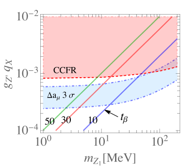
Figure 1: Parameter space preferred by the muon $g-2$ (shaded region bounded by blue dot-dashed curves) and ruled out by the CCFR experiment (shaded region above the red dashed curve). The solid lines represent the contours for $t_{\beta}$.

The SM prediction for the Higgs boson width is $\Gamma^{\rm SM}_{h}\approx 4.1$ MeV LHCHiggsCrossSectionWorkingGroup:2016ypw , while the current measurement gives $\Gamma^{\rm exp}_{h}=3.2^{+2.8}_{-2.2}$ MeV PDG2022 . As an illustrated example, we assume that each new Higgs decay channel in the model contributes less than $5\%$ of $\Gamma^{\rm SM}_{h}$, i.e., $\Gamma^{\rm NP}_{h}\leq 0.20$ MeV. This assumption is consistent with the current upper limit on the Higgs invisible decays, $BR(h\to\text{invisible})<0.19$ PDG2022 . To fit the observed Higgs signal strengths, the Higgs couplings to the fermions and the $W^{\pm}$ and $Z$ gauge bosons should have $s_{\beta-\alpha}\approx 1$.

We now use $\Gamma(h\to HH)$ to bound $c_{\beta-\alpha}$ and $t_{\beta}$. Since the $h\to HH$ process depends on $m_{H}$, we show the upper bound on $\xi$, defined in Eq. (53), for some benchmarks of $m_{H}$:

$$\xi\lesssim\frac{10^{-3}\Gamma(h\to HH)}{\text{0.20 MeV}}\times\left\{\begin{array}[]{cc}0.59&\text{$m_{H}=30$ GeV}\,,\\ 0.61&\text{$m_{H}=50$ GeV}\,,\\ 1.07&\text{$m_{H}=60$ GeV}\,.\end{array}\right.$$ (67)

To illustrate the dependence of $\xi$ on $c_{\beta-\alpha}$ and $t_{\beta}$, we show in Fig. 2 the contour plot of $\xi$ in the $t_{\beta}$-$c_{\beta-\alpha}$ plane, where we have fixed $\xi=0.61\times 10^{-3}$ and $\Gamma(h\to HH)=0.20$ MeV. It is found that there are two slightly separated contours, which are insensitive to the chosen value of $\xi$ and indicate that $c_{\beta-\alpha}$ decreases as $t_{\beta}$ increases. With the choice of $t_{\beta}=25$, $m_{H}=50$ GeV, and $\xi=0.61\times 10^{-3}$, we obtain $c_{\beta-\alpha}\approx 4.095\%$ and $s_{\beta-\alpha}\approx 99.92\%$. The values in turn determine that $\Gamma(h\to Z_{1}Z_{1})\approx 0.17$ MeV and $\Gamma(h\to Z_{1}Z_{2})\approx 0.11$ MeV.

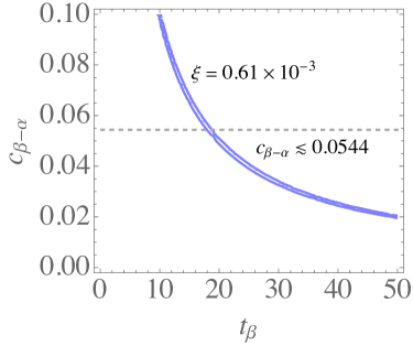
Figure 2: Contours of $\xi$ (blue solid curves) in the $t_{\beta}$-$c_{\beta-\alpha}$ plane, assuming $\xi=0.61\times 10^{-3}$ and $\Gamma(h\to HH)=0.20$ MeV. The dashed line denotes the upper bound on $c_{\beta-\alpha}$ from $\Gamma(h\to Z_{1}Z_{2})\leq 0.20$ MeV.

In the large $t_{\beta}$ scheme now, $\Gamma(h\to Z_{1}Z_{2})$ only depends on $c_{\beta-\alpha}$. With $m_{h}=125$ GeV and $m_{Z_{2}}=91.187$ GeV, the limit of $c_{\beta-\alpha}$ can be determined as:

$$c_{\beta-\alpha}\lesssim 0.0544\left(\frac{\Gamma(h\to Z_{1}Z_{2})}{\text{0.20 MeV}}\right)^{1/2}\,.$$ (68)

The assumption of $\Gamma(h\to Z_{1}Z_{2})\leq 0.20$ MeV then translates into the dashed line in Fig. 2. According to the result in Eq. (21), we can estimate the $Z^{\prime}-Z$ mixing angle to have:

$$|s_{\theta_{Z}}|\approx 1.08\times 10^{-5}\left(\frac{20}{t_{\beta}}\right)\left(\frac{m_{Z_{1}}}{\text{20 MeV}}\right)\,.$$ (69)

Clearly, $s_{\theta_{Z}}$ can be larger than the loop-induced kinetic mixing between $Z^{\prime}$ and $\gamma$, characterized by the mixing parameter Holdom:1985ag ; Chen:2017cic :

$$\epsilon=\frac{g_{Z^{\prime}}e}{6\pi^{2}}\ln\frac{m_{\tau}}{m_{\mu}}\approx 8.68\times 10^{-6}\left(\frac{g_{Z^{\prime}}}{6\times 10^{-4}}\right)\,.$$ (70)

Consequently, we concentrate on the contributions from the $Z^{\prime}-Z$ mixing in this study.

The $\chi_{\mu\tau}$ parameter is related to the $h\to\mu\tau$ and $\tau\to\mu Z_{1}$ decays and $\Delta a^{H}_{\ell}$. Since the $\tau\to\mu Z_{1}$ process is strongly enhanced by $m^{2}_{\tau}/m^{2}_{Z_{1}}$, its measurement will put a strict constraint on $\chi_{\mu\tau}$. To bound the $\chi_{\mu\tau}$ parameter, we can use the upper limit of the process $\tau\to\mu+\text{light boson}$ as an estimate, where the current data give $BR(\tau\to\mu+\text{light boson})<5\times 10^{-3}$ PDG2022 ; Belle-II:2022heu . With $c_{\theta_{L}}\approx c_{\theta_{Z}}\approx 1$ and the result in Eq. (56), we obtain an upper bound on $\chi_{\mu\tau}$ as:

$$\chi_{\mu\tau}<1.82\times 10^{-5}\left(\frac{25}{t_{\beta}}\right)\,.$$ (71)

The resulting $BR(h\to\mu\tau)$ and $\Delta a^{H}_{\mu}$ are then less than ${\cal O}(10^{-11})$ and ${\cal O}(10^{-16})$, respectively.

The primary purpose of introducing the LQ, $S^{1/3}$, in the model is to address the $R(D^{(*)})$ anomalies. Along with the mass of LQ, the related parameters are $y^{q}_{L3,L2}$, $y^{u}_{R2}$, and $V^{\ell}_{L\ell\tau}$. Due to the $\tau\to\mu Z_{1}$ constraint, the lepton-flavor mixing matrix can be approximated as $V^{\ell}_{L}\approx 1$, allowing us to ignore its contribution to the muon mode. Consequently, the LQ only couples to the third-generation leptons. According to Eq. (34), unlike the independent couplings to the different up-type quarks, the LQ couplings to the different flavor down-type quarks are related by the CKM matrix and can be written as:

$$(V^{T}_{\rm CKM}{\bf y}^{q}_{L})_{d} \approx\frac{10}{3}\lambda^{4}y^{q}_{L3}-\lambda y^{q}_{L2}+y^{q}_{L1}\,,$$

$$(V^{T}_{\rm CKM}{\bf y}^{q}_{L})_{s} \approx-\frac{4}{5}\lambda^{2}y^{q}_{L3}+y^{q}_{L2}+\lambda y^{q}_{L1}\,,$$

$$(V^{T}_{\rm CKM}{\bf y}^{q}_{L})_{b} \approx y^{q}_{L3}\,,$$ (72)

where $\lambda\approx 0.2257$ is a Wolfenstein parameter and $V_{ub}\ll V_{cb}\ll V_{tb}\approx V_{cs}\approx V_{ud}\approx 1$ has been applied. To suppress the LQ couplings to the first- and second-generation quarks so as to satisfy constraints from low-energy physics, such as $P-\bar{P}$ mixing and $q_{i}\to q_{j}\bar{f}^{\prime}f^{\prime}$, where $P$ and $f^{\prime}$ are respectively possible neutral mesons and leptons, we require the Yukawa couplings to have the hierarchy:

$$y^{q}_{L3}\sim{\cal O}(1)\,,~{}y^{q}_{L2}\sim{\cal O}(\lambda^{2})\,,~{}y^{q}_{L1}\sim{\cal O}(\lambda^{3})~{}.$$ (73)

If cancellations are allowed in the terms of $(V^{T}_{\rm CKM}{\bf y}^{q}_{L})_{d,s}$, small LQ couplings to the first two generations of down-type quarks can be easily achieved in the model. Although $D-\bar{D}$ mixing can constrain $y^{u}_{R2}y^{u}_{R1}$, we can take a small $y^{u}_{R1}$ to avoid this constraint on $|y^{u}_{R2}|$, for which we need $y^{u}_{R2}\sim{\cal O}(0.5)$ to enhance $R(D^{(*)})$.

In this model, the LQ couplings to the third-generation quarks are dominant. Both CMS CMS:2020wzx and ATLAS ATLAS:2021oiz have searched for the scalar LQ with a charge of $e/3$ using the $t\tau$ and $b\nu$ production channels. ATLAS has placed a stronger upper bound on the LQ mass when $BR(S^{-1/3}\to t\tau)=1/2$, obtaining $m_{S}\geq 1.22$ TeV. If we set $y^{u}_{R3}=0$, then the ATLAS measurement can be directly applied to our model and we thus assume that $t\tau$ and $b\nu_{\tau}$ are the dominant decays of the LQ. To be more conservative, we use $m_{S}=1.5$ TeV in our numerical calculations.

IV.2 Phenomenological Analysis

Here we present the numerical results of the observables discussed in Sec. III and highlight their features, while taking into account the constrained parameter space obtained in Sec. IV.1.

IV.2.1 Cross sections of CE$\nu$NS on Ar and CsI targets

Since the targets of the measured coherent elastic neutrino scattering in the COHERENT experiment are Ar and CsI, we focus on both targets in the following numerical analysis. Because CsI is a compound of cesium and iodide, the fraction of each nucleus contributing to the cross section is defined by $f_{i}=A_{i}/(A_{\rm Cs}+A_{\rm Ar})$ AristizabalSierra:2019zmy . Based on COHERENT’s best-fit results for $\langle\sigma\rangle_{e}$ and $\langle\sigma\rangle_{\mu+\bar{\mu}}$ COHERENT:2021xmm , where the resulting $\langle\sigma\rangle_{\mu+\bar{\mu}}$ is noticeably smaller than the SM prediction, we choose to present the numerical results with sign$(\theta_{Z})=-1$.

Using Eq. (44), we show the total cross section of CE$\nu$NS for Ar (solid) and CsI (dashed) as a function of $m_{Z_{1}}$ in Fig. 3(a). We estimate the SM results for Ar and CsI to be $18.2\times 10^{-40}$ cm² and $183.12\times 10^{-40}$ cm², respectively. Since the cross section is plotted in the logarithmic scale, the sensitivity in $m_{Z_{1}}$ is not obvious. To illustrate the new physics effects, we show the deviation from the SM result, defined by ($\langle\sigma^{\rm NP+SM}\rangle_{\phi}-\langle\sigma^{\rm SM}\rangle_{\phi})/\langle\sigma^{\rm SM}\rangle_{\phi}$, in Fig. 3(b). It can be seen that the influence of new physics can exceed $10\%$ when $m_{Z_{1}}\gtrsim 12$ MeV, with a slightly larger influence on CsI than on Ar.

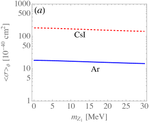
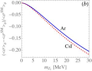
Figure 3: (a) Cross section averaged by neutrino fluxes for Ar and CsI targets as a function of $m_{Z_{1}}$, where the points for $m_{Z_{1}}=0$ correspond to the SM results. (b) Fractional deviation on the total cross section $\langle\sigma\rangle_{\phi}$ from its SM value as a function of $m_{Z_{1}}$. In both plots, the solid and dashed curves represent the results for Ar and CsI targets, respectively.

In addition to the total cross section of CE$\nu$NS, the cross section at specific incident neutrino energy $E_{\nu}$ serves as another useful physical observable for probing the new physics effects. For clarity, we define the averaged total cross section as a function of $E_{\nu}$ as follows:

$$\langle\Sigma\rangle =\frac{1}{\Phi(E_{\nu})}\sum_{\ell=e,\mu,\bar{\mu}}\int^{E^{\rm max}_{r}}_{E^{\rm min}_{r}}dE_{r}\frac{d\sigma(\nu_{\ell}A\to\nu_{\ell}A)}{dE_{r}}\frac{d\phi_{\ell}(E_{\nu})}{dE_{\nu}}\,,$$

$$\Phi(E_{\nu}) =\sum_{\ell=e,\mu,\bar{\mu}}\frac{d\phi_{\ell}(E_{\nu})}{dE_{\nu}}\,.$$ (74)

In Fig. 4(a), we show $\langle\Sigma\rangle$ as a function of $E_{\nu}$ in the SM for the targets of Ar, I, and Cs by the solid, dot-dashed, and dashed curves, respectively. To demonstrate the sensitivity of $\langle\Sigma\rangle$ to the new physics effects, we present the results for Ar and CsI in Figs. 4(b) and (c), respectively, where the solid, dot-dashed, and dashed curves denote cases with $m_{Z_{1}}=(0,10,30)$ MeV. It can be seen that the deviation from the SM increases with $m_{Z_{1}}$. To illustrate the sensitivity of $\langle\Sigma\rangle$ on the $Z^{\prime}$ mass, we exhibit $\delta\langle\Sigma\rangle=(\langle\Sigma^{\rm NP+SM}\rangle-\langle\Sigma^{\rm SM}\rangle)/\langle\Sigma^{\rm SM}\rangle$ in Fig. 4(d) for Ar and CsI, where the dot-dashed and dashed curves are for $m_{Z_{1}}=10$ and $30$ MeV. From the results, we find that the sensitivity level $|\delta\langle\Sigma\rangle|$ first decreases with $E_{\nu}$ increases and then turn to increase with $E_{\nu}$ at some higher $E_{\nu}$, e.g. at $E_{\nu}\sim(41,36)$ MeV for $m_{Z_{1}}=(10,30)$ MeV. Hence, the deviation from the SM result can reach $\sim 11\%$ ($22\%$) at $E_{\nu}=15$ MeV and $\sim 7\%$ ($25\%$) at $E_{\nu}=50$ MeV for $m_{Z_{1}}=10~{}(30)$ MeV.

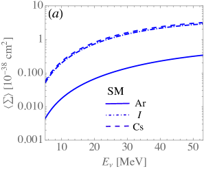
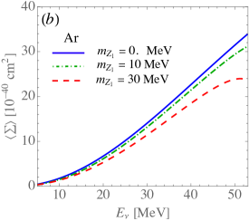
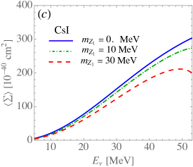
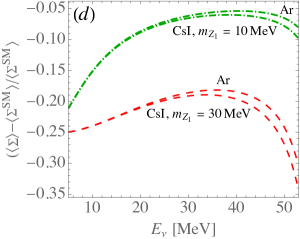
Figure 4: (a) $\langle\Sigma\rangle$ as a function of $E_{\nu}$ for Ar (solid), I (dot-dashed) , and Cs (dashed) in the SM. $\langle\Sigma\rangle$ for (b) Ar and (c) CsI with $m_{Z_{1}}=0$ MeV (solid), $10$ MeV (dot-dashed), and $30$ MeV (dashed). (d) Sensitivity of $\langle\Sigma\rangle$ on the $Z^{\prime}$ boson for Ar and CsI with $m_{Z_{1}}=10$ MeV (dot-dashed) and $30$ MeV (dashed).

IV.2.2 $R(D)$ and $D(D^{*})$ mediated by LQ

The calculations of $R(D)$ and $R(D^{*})$ depend on the form factors of the $B\to(D,D^{*})$ transitions. In the study, we use the form factors given in Ref. Bernlochner:2017jka , obtained using the heavy quark effective theory (HQET). With the input values of $m_{B^{+}}=5.28~{}{\rm GeV}$, $m_{D^{0}}=1.864~{}{\rm GeV}$, $m_{D^{0*}}=2.007~{}{\rm GeV}$, $\tau_{B^{-}}=2.450\times 10^{12}~{}{\rm GeV}^{-1}$, and $V_{ub}=0.0395$, the BRs for $B^{+}\to(D^{0},D^{0*})\ell\nu$ are found to be consistent with current experimental data, as shown in Table 2. Using the formulas presented in Sec. III.2, we obtain for the SM that:

$$R^{\rm SM}(D)\approx 0.297\,,~{}R^{\rm SM}(D^{*})\approx 0.258\,.$$ (75)

The values are within $1\sigma$ errors of those obtained in Ref. Bernlochner:2017jka and are consistent with the results given in Refs. MILC:2015uhg ; Na:2015kha ; Bigi:2016mdz ; Bernlochner:2017jka ; Jaiswal:2017rve ; BaBar:2019vpl ; Bordone:2019vic ; Martinelli:2021onb .

Table 2: Branching ratios of the $B^{-}\to D^{0(*)}\ell\nu$ decays in the SM and their experimental measurements.

Mode	$B^{-}\to D^{0}\ell\nu$	$B^{-}\to D\tau\nu$	$B^{-}\to D^{0*}\ell\nu$	$B^{-}\to D^{0*}\tau\nu$
SM	$2.32\%$	$6.89\times 10^{-3}$	$5.84\%$	$1.50\%$
Exp PDG2022	$(2.30\pm 0.09)\%$	$(7.7\pm 2.5)\times 10^{-3}$	$(5.58\pm 0.22)\%$	$(1.88\pm 0.20)\%$

The parameters involved in the $b\to c\tau\nu$ transitions mediated by the LQ appear in the combinations of $y^{q}_{L3}y^{q}_{L2}/m^{2}_{S}$ and $y^{q}_{L3}y^{u}_{R2}/m^{2}_{S}$. For the numerical analysis, we fix $m_{S}=1.5$ TeV. From Eq. (72), we see that $y^{q}_{L2}\sim{\cal O}(\lambda^{2})\ll y^{q}_{L3}$, indicating that the dominant effect on $R(D)$ and $R(D^{*})$ comes from the combination $y^{q}_{L3}y^{u}_{R2}$. To simplify the analysis, we take the assumption that $y^{q}_{L2}=0$, in which case $R(D^{(*)})$ is found to deviate from that with $y^{q}_{L2}=0.04$ by only $\sim 2\%$. We present the contours of $R(D)$ and $R(D^{*})$ in the $y^{q}_{L3}$-$y^{u}_{R2}$ plane in the left plot of Fig. 5, with the shaded areas (light-green and grey, respectively) covering the $2\sigma$ ranges of their world averages. It is seen that the low boundaries of $R(D)$ and $R(D^{*})$ match exactly, while the upper boundary for $R(D)=0.414$ is close to the contour of $R(D^{*})=0.297$. This illustrates that an accurate measurement of $R(D)$ can indirectly constrain the value of $R(D^{*})$, and vice versa. The right plot of Fig. 5 shows the dependence of $R(D^{(*)})$ on the product $y^{q}_{L3}y^{u}_{R2}$. To explain the $R(D)$ and $R(D^{*})$ anomalies, we need $-1<y^{q}_{L3}y^{u}_{R2}<0$ for $m_{LQ}=1.5$ TeV. It is observed that $R(D)$ is more sensitive to the $S^{1/3}$ contribution.

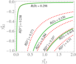
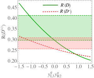
Figure 5: Left: Contours of $R(D)$ and $R(D^{*})$ in the $y^{q}_{L3}$-$y^{u}_{R2}$ plane. The solid (darker-green) and dashed (red) lines cover the $2\sigma$ range of the world-averaged $R(D)$ and $R(D^{*})$, respectively. Right: Dependence of $R(D^{(*)})$ on $y^{q}_{L3}y^{u}_{R2}$. The light-green [pink] shaded region represents the $2\sigma$ range of the world-averaged $R(D)$ [$R(D^{*})$].

In addition to the ratio of the BR for $\tau\nu$ to that for $\ell\nu$, there are other physical observables that may be sensitive to new physics, such as forward-backward asymmetry of the charged lepton, $\tau$-polarization Chen:2017eby ; Chen:2018hqy , and $q^{2}$-dependent differential decay rates. The BR is sensitive to the CKM matrix elements and the form factors of the $B\to(D,D^{*})$ transitions. To eliminate these factors, we propose the ratio of the $q^{2}$-dependent differential decay rates, defined to be:

$$R_{M}(q^{2})=\frac{d\Gamma^{\tau}_{M}/dq^{2}}{d\Gamma^{\ell^{\prime}}_{M}/dq^{2}}H(q^{2}-m^{2}_{\tau})\,,$$ (76)

where $H(x)$ is the Heaviside step function, and $d\Gamma^{\ell^{\prime}}_{M}/dq^{2}$ is the average of the electron and muon modes. Because the threshold invariant mass-squared of $\tau\nu$ in the $B\to M\tau\nu$ decay is $q^{2}=m^{2}_{\tau}$, we thus require that the denominator $d\Gamma^{\ell^{\prime}}_{M}/dq^{2}$ also starts from the same invariant mass-squared. To appreciate the benefit of considering the observable defined in Eq. (76), we first show the $q^{2}$-dependent BRs for $B^{-}\to(D^{0},D^{0*})\ell\nu$ in the SM in Figs. 6(a) and (b). Plot (a) shows that when $q^{2}\gtrsim 8$ GeV², the decay $B^{-}\to D^{0}\tau\nu$ becomes larger than the light lepton mode, and it is expected that $R_{D}(q^{2})>1$ in this region. $D^{*}$ is a vector meson and has longitudinal ($P_{L}$) and transverse ($P_{T}$) components. To exhibit their contributions, we separately show $P_{L}$ and $P_{T}$ in Fig. 6 (b). The results indicate that $P_{T}$ becomes larger than $P_{L}$ at somewhat large $q^{2}$ regions in both light lepton and $\tau$ modes. In contrast to the $B^{-}\to D^{0}\ell\nu$ decay, $d\Gamma^{\ell^{\prime}}_{D^{*}}/dq^{2}$ is always larger than $d\Gamma^{\tau}_{D^{*}}/dq^{2}$ in the allowed kinematic region, thus, it is expected that $R_{D^{*}}(q^{2})<1$.

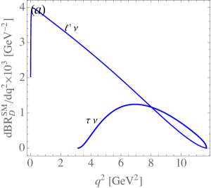
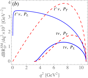
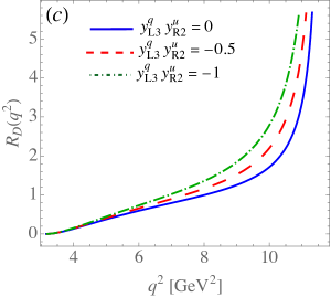
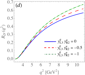
Figure 6: Differential BR as a function of $q^{2}$ in the SM for (a) $B^{-}\to D^{0}\ell^{\prime}\nu$ and (b) $B^{-}\to D^{*}\tau\nu$. The ratios $R_{D}(q^{2})$ (c) and $R_{D^{*}}(q^{2})$ (d) as functions of $q^{2}$, where the solid, dashed, and dot-dashed curves are for $y^{q}_{L3}y^{u}_{R2}=0$, $-0.5$, and $-1$, respectively.

The $q^{2}$-dependence of $R_{D}(q^{2})$ and $R_{D^{*}}(q^{2})$ in the SM is shown in Figs. 6(c) and (d), respectively, using the solid curves. It is confirmed that $R_{D}(q^{2})\gtrsim 1$ at $q^{2}\gtrsim 8$ GeV, while $R_{D^{*}}(q^{2})<1$ in the physical kinematic region. Additionally, we find that $R_{M}(q^{2})$ increases monotonically with $q^{2}$. This means that the decreasing rate of $d\Gamma^{\ell^{\prime}}_{M}/dq^{2}$ in $q^{2}$ is faster than that of $d\Gamma^{\tau}_{M}/dq^{2}$. To see how sensitive $R_{M}(q^{2})$ is to new physics effects, we show the results using benchmarks of $y^{q}_{L3}y^{u}_{R2}=-0.5$ (dashed) and $y^{q}_{L3}y^{u}_{R2}=-1$ (dot-dashed) for $R_{D}(q^{2})$ and $R_{D^{*}}(q^{2})$ in the corresponding plots. We also consider the quantity $(R^{\rm NP}_{M}(q^{2})-R^{\rm SM}(q^{2}))/R^{\rm SM}_{M}(q^{2})$ to show the deviation caused by the new physics effects in $R_{M}(q^{2})$ from the SM result, and show the results in Fig. 7. The variations of these curves show that $R_{D}(q^{2})$ is more sensitive to new physics than $R_{D^{*}}(q^{2})$ in the model.

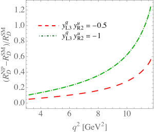
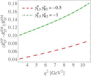
Figure 7: Deviation of $R_{M}(q^{2})$ from the SM result for $B^{-}\to D^{0}\ell\nu$ (left) and $B^{-}D^{0*}\ell\nu$ (right).

IV.2.3 The oblique parameters and $W$-mass

By combining the CDF II measurement of $m_{W}$ with others, the oblique parameters are determined to be deBlas:2022hdk :

$$U \equiv 0\,,~{}S=0.10\pm 0.073\,,~{}T=0.202\pm 0.056\,,$$

$$U =0.134\pm 0.087\,,~{}S=0.05\pm 0.096\,,~{}T=0.040\pm 0.120\,.$$ (77)

We can use these results to constrain the free parameters in the model. Based on Eqs. (59), (61), and (62), the oblique parameters have a quadratic dependence on $c_{\beta-\alpha}$. However, $c_{\beta-\alpha}\lesssim{\cal O}(0.04)$ as previously discussed, meaning that its effects on the $S$, $T$, and $U$ parameters are negligible. Therefore, these parameters can be approximated for the model as follows:

$$T \simeq\frac{1}{16\alpha_{\rm em}\pi^{2}v^{2}}s^{2}_{\beta-\alpha}F(m^{2}_{H^{+}},m_{H})\,,$$

$$S \simeq\frac{1}{24\pi}\left[(c^{2}_{W}-s^{2}_{W})^{2}G(m^{2}_{H^{+}},m^{2}_{H^{+}},m^{2}_{Z})+\ln\frac{m^{2}_{H^{+}}}{m^{2}_{H}}\right]\,,$$

$$U \simeq\frac{1}{24\pi}\left[s^{2}_{\beta-\alpha}G(m^{2}_{H^{+}},m^{2}_{H},m^{2}_{W})-(2s^{2}_{W}-1)^{2}G(m^{2}_{H^{+}},m^{2}_{H^{+}},m^{2}_{Z})\right]\,.$$ (78)

In this simplified form, the oblique parameters depend only on the ratio $m_{H^{+}}/m_{H}$. The contours for $S$ (solid), $T$ (dashed), and $U$ (dot-dashed) in the plane of $m_{H^{+}}$ and $m_{H}$ for the model are drawn in Fig. 8(a), where $s_{\beta-\alpha}\approx 1$ is taken in the estimates. From the results, the values of $S$ and $U$ in the model can only be up to the percent level and can be neglected in the numerical estimates for futher phenomenological analysis. Thus, using the obtained $T$ parameter, the loop-corrected $W$ mass in the model is shown in Fig. 8(b), where the contours correspond to the central value, $\pm 2\sigma$ and $\pm 5\sigma$ of the world average of $m_{W}=80.4133\pm 0.0080$ deBlas:2022hdk . We observe that $m_{W}$ increases with $m_{H^{+}}$ for a given $m_{H}$, while a lower $m_{H}$ is needed to increase $m_{W}$ when $m_{H^{+}}$ is fixed. For instance, $m_{W}\approx 80.43$ GeV can be achieved as $m_{H}\approx 50$ GeV and $m_{H^{+}}\approx 150$ GeV.

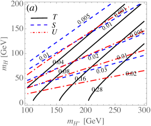
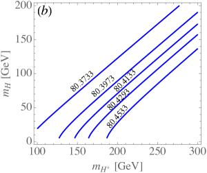
Figure 8: (a) Contours of the oblique parameters, $S$, $T$, and $U$, in the $m_{H}$-$m_{H^{+}}$ plane. (b) Contours of $m_{W}$ in the $m_{H}$-$m_{H^{+}}$ plane.

IV.2.4 $Z_{1}$ and $H$ decays

Finally, let’s discuss possible decays of light $Z_{1}$ and $H$. Because the mass of the light gauge boson is limited in the region of $m_{Z_{1}}\in(10,100)$ MeV, it can only decay dominantly into on-shell light leptons through two-body decay. The $Z_{1}$ partial decay rate for possible final leptons is given by:

$$\Gamma(Z_{1}\to f\bar{f})\simeq\frac{g^{2}m_{Z_{1}}}{96c^{2}_{W}}\left(|C^{f}_{R}|^{2}+|C^{f}_{L}|^{2}\right)\,,$$ (79)

where $C^{f}_{R(L)}=C^{f}_{1V}\mp C^{f}_{1A}$, $f$ denotes the possible light leptons (such as the three active neutrinos and electron), and $m^{2}_{f}/m^{2}_{Z_{1}}\approx 0$ is applied. The effective couplings of $C^{f}_{R,L}$ for each involved $f$ are given as follows:

$$C^{\nu_{\ell}}_{R} =0~{},~{}C^{\nu_{e}}_{L}=s_{\theta_{Z}}~{},$$

$$C^{\nu_{\mu,\tau}}_{L} =s_{\theta_{Z}}\pm\frac{c_{W}m_{Z_{1}}c_{\theta_{Z}}}{gv}\sqrt{2+t^{2}_{\beta}+t^{-2}_{\beta}}\,,$$ (80)

$$C^{e}_{R} =2s^{2}_{W}s_{\theta_{Z}}\,,~{}C^{e}_{L}=(-1+2s^{2}_{W})s_{\theta_{Z}}\,.$$

Although $Z^{\prime}$ does not couple to the first-generation leptons, the physical $Z_{1}$ can decay to them via $Z^{\prime}-Z$ mixing.

If $s_{\theta_{Z}}$ were not significantly smaller than $g_{Z^{\prime}}$, the decay rates for $Z_{1}\to(\bar{\nu}_{e}\nu_{e},\,e^{-}e^{+})$ could be sizable compared to the $Z_{1}\to\bar{\nu}_{\ell^{\prime}}\nu_{\ell^{\prime}}$ decays. However, due to the large $t_{\beta}$ enhancement in the $Z_{1}$ gauge coupling to $\nu_{\mu,\tau}$, the dominant decay channels are $Z_{1}\to\nu_{\mu}\bar{\nu}_{\mu}/\nu_{\tau}\bar{\nu}_{\tau}$, with estimated BRs of approximately $50.5\%$ and $49.5\%$, respectively. The BRs for $\nu_{e}\bar{\nu}_{e}$ and $e^{-}e^{+}$ as functions of $t_{\beta}$ are presented in Fig. 9(a). It is found that the BRs are more sensitive to $t_{\beta}$ and less sensitive to $m_{Z_{1}}$. Because $Z_{1}$ can be produced in the $\tau\to\mu Z_{1}$ decay, which depends on the lepton-flavor mixing $\theta_{L}$, a significant $BR(Z_{1}\to e^{-}e^{+})$ thus implies a large BR for the LFV process $\tau\to\mu Z_{1}\to\mu e^{-}e^{+}$, where the current upper limit is $BR(\tau\to\mu e^{-}e^{+})<1.8\times 10^{-8}$ PDG2022 . Our estimate of $BR(\tau\to\mu e^{-}e^{+})$ is shown in Fig. 9(b), where $\chi_{\mu\tau}=10^{-5}$ is used. Since $\tau\to\mu Z_{1}$ is also not sensitive to $m_{Z_{1}}$, the dependence of $m_{Z_{1}}$ in $BR(\tau\to\mu e^{-}e^{+})$ is not manifest. Assuming the integrated luminosity of $50$ ab^-1, Belle II will be capable of probing the LFV process BRs down to the level of $10^{-10}-10^{-9}$ Banerjee:2022vdd . The BR of ${\cal O}(10^{-9})$ for $\tau\to\mu e^{-}e^{+}$ predicted in this model can thus be probed at Belle II.

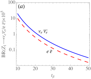
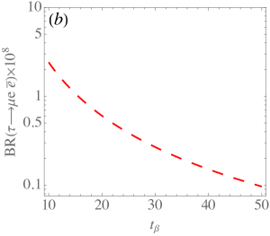
Figure 9: BRs for (a) $Z_{1}\to(\nu_{e}\bar{\nu}_{e},e\bar{e})$ and (b) $\tau\to\mu Z_{1}\to\mu e^{-}e^{+}$ as functions of $t_{\beta}$.

As discussed earlier, when $m_{H}<m_{h}/2$, $H$ can be produced through the $h\to HH$ decay. The partial decay width of this process can provide a strict limit on the $t_{\beta}$ and $c_{\beta-\alpha}$ parameters. In the following, we concentrate on this scenario, even though $H$ generally can be heavier.

For two-body decays, $H$ should decay into a pair of fermions, as long as the phase space permits. From Eq. (25), its Yukawa couplings to fermions are suppressed by $m_{f}/v$ and $(c_{\beta-\alpha}-t_{\beta}s_{\beta-\alpha})$, with no other factors that can enhance the partial decay width. As a result, $\Gamma(H\to f\bar{f})$ is small and negligible. However, even though suppressed by $m^{2}_{Z_{1}}/v$ from the gauge coupling as shown in

$${\cal L}_{HZ_{1}Z_{1}}\simeq\frac{2(t^{2}_{\beta}-1)}{t_{\beta}}\frac{m^{2}_{Z_{1}}}{v}s_{\beta-\alpha}\frac{HZ_{1\mu}Z^{\mu}_{1}}{2}\,,$$ (81)

the $H\to Z_{1}Z_{1}$ decay rate can be enhanced by the longitudinal component, which is proportional to $1/m_{Z_{1}}$. This leads to a partial decay width,

$$\Gamma(H\to Z_{1}Z_{1})\simeq\frac{m_{H}}{32\pi}\frac{m^{2}_{H}}{v^{2}}\left|\frac{t^{2}_{\beta}-1}{t_{\beta}}s_{\beta-\alpha}\right|^{2}\,.$$ (82)

The original suppression factor from the gauge coupling is seen to be canceled by the longitudinal effect of $1/m^{2}_{Z_{1}}$ from each $Z_{1}$ boson. With $m_{H}=50$ GeV and $t_{\beta}=20$, we obtain $\Gamma(H\to Z_{1}Z_{1})\approx 8.2$ GeV. The other decay processes are subdominant. For example, the $H\to Z_{1}Z^{*}_{2}\to Z_{1}f\bar{f}$ decay has additional suppression factors due to the phase space and $1/m^{2}_{Z_{2}}$. An explicit estimate shows that the partial width for $H\to Z_{1}Z^{*}_{2}$ is of ${\cal O}(10^{-5})$. According to the earlier analysis, $Z_{1}\to\nu\bar{\nu}$ is the dominant decay channel. Consequently, $H$ predominantly decays into invisible neutrinos and becomes missing energy in the detector.

We now turn to the production of $H$ at the LHC. First, $H$ could also be singly produced according to Eq. (22) via the vector boson fusion (VBF) processing. But the $W^{-}W^{+}(ZZ)H$ coupling is suppressed by $c_{\beta-\alpha}$. Additionally, the Yukawa coupling for the bremsstrahlung production of $H$ with the top quark is determined by $(m_{t}/v)(c_{\beta-\alpha}-s_{\beta-\alpha}/t_{\beta})$ and is also suppressed. However, $H$ can be pair-produced more copiously through the $hHH$ and $W^{-}H^{+}H$ couplings. In the former case, the $H$ pair is produced by the on-shell Higgs boson, i.e., $pp\to h\to HH$. From Eq. (53), although $\Gamma(h\to HH)$ is associated with the small factor $\xi$, its BR can still be at the percent level. This amounts to the invisible decay of the Higgs boson ATLAS:2022yvh . In the latter case, the $W^{-}H^{+}H$ coupling, as given in Eq. (22), is determined by the gauge coupling $g$ with $s_{\beta-\alpha}\approx 1$. When $H^{+}$ is taken as an intermediate state in the t-channel scattering, $H$ pair production occurs via the VBF channel, i.e., $pp\to HH+{\rm jets}$. We may probe such an effect by the search for invisible decays of the new scalar $H$ ATLAS:2022yvh .

V Summary

Motivated by the observation of coherent elastic neutrino-nucleus scattering (CE$\nu$NS) measured by the COHERENT experiment, we have studied in this work an extension of the SM with a gauged $U(1)_{\mu-\tau}$ symmetry. To dynamically break the new $U(1)$ gauge symmetry and to accommodate several other observed anomalies, such as the muon $g-2$, $R(D)$ and $R(D^{*})$, and the $W$ mass deviation, we introduce a new Higgs doublet and a scalar singlet leptoquark $S^{1/3}$.

In such a two-Higgs-doublet model, two Goldstone bosons serve as the longitudinal components of the $Z$ and $Z^{\prime}$ bosons. As a result, the physical scalar states include two CP-even Higgs and one charged Higgs boson. With the new Higgs doublet carrying also the $U(1)_{\mu-\tau}$ charge, the mixing between the new scalar boson and the SM-like Higgs leads to new decay channels for the Higgs boson, including $h\to\mu\tau/Z_{1}Z_{1}/Z_{1}Z_{2}$ (and $h\to HH$ when $m_{H}<m_{h}/2$). It was found that the $\tau\to\mu Z_{1}$ decay strictly constrains the $\mu-\tau$ flavor mixing, resulting in a highly suppressed $h\to\mu\tau$ decay. By assuming proper partial widths to the new Higgs decay channels, the $\tan\beta$ and $\cos(\beta-\alpha)$ parameters are limited, and the large $\tan\beta$ scheme is favored. Although the $\mu-\tau$ flavor-changing coupling is restricted to be small, the $\tau\to\mu Z_{1}\to\mu e^{-}e^{+}$ decay can still reach the sensitivity of ${\cal O}(10^{-9})$ at Belle II.

Taking into account all potential constraints, we have found that the cross section of CE$\nu$NS induced by the $Z^{\prime}-Z$ mixing depends solely on the light gauge boson mass, $m_{Z_{1}}$. The mass region of $m_{Z_{1}}$ that is used to fit the CE$\nu$NS cross section, measured by COHERENT using the CsI target COHERENT:2021xmm , can also explain the muon $g-2$ anomaly within $3\sigma$. To demonstrate the sensitivity of new physics to CE$\nu$NS in the model, we propose to study the cross section as a function of the incident neutrino energy. Our results show that in the low energy region, such as $E_{\nu}\sim 10$ MeV, the deviation from the SM can exceed $15\%$, depending on the value of $m_{Z_{1}}$.

In addition to explaining the observed excesses in $R(D)$ and $R(D^{*})$ using the introduced leptoquark, we have proposed a $q^{2}$-dependent ratio of $d\Gamma/dq^{2}(B\to M\tau\nu)$ to $d\Gamma/dq^{2}(B\to M\ell\nu)$, denoted by $R_{M}(q^{2})$. Our results show that in the high $q^{2}$ region, $R_{D}(q^{2})$ is more sensitive to the new physics effects and exhibits a significant deviation from the SM.

We have also studied the impact of the two-Higgs-doublet model on the oblique parameters and their relations to the $W$ boson mass. With the approximation that $\cos(\beta-\alpha)\ll 1$, the parameters involved in the oblique parameters are $m_{H}$ and $m_{H^{+}}$. We find that there is a significant space in the $m_{H}$-$m_{H^{+}}$ plane that allows an enhancement of $m_{W}$ up to the value observed by CDF II. Finally, we have discussed the possible decay channels for $Z_{1}$ and $H$ in the scenario where $m_{Z_{1}}\in(10,100)$ MeV and $m_{H}<m_{h}/2$. The analysis shows that $Z_{1}\to\nu_{\mu}\bar{\nu}_{\mu}/\nu_{\tau}\bar{\nu}_{\tau}$ and $H\to Z_{1}Z_{2}$ are the dominant decay channels.

Appendix A $\bar{B}\to D^{(*)}$ transition form factors

A.1 Form factor parameterization

In this section, we define the $\bar{B}\to D^{(*)}$ transition form factors for the $\bar{B}\to D^{(*)}\ell\nu$ decays. First, the transition form factors associated with the various currents mediating the $\bar{B}\to D$ transitions are parametrized as:

$$\langle D(p_{2})|qb|\bar{B}(p_{1})\rangle =(m_{B}+m_{D})F_{S}(q^{2})\,,$$

$$\langle D(p_{2})|q\gamma^{\mu}b|\bar{B}(p_{1})\rangle =F_{+}(q^{2})\left((p_{1}+p_{2})^{\mu}-\frac{m^{2}_{B}-m^{2}_{D}}{q^{2}}q^{\mu}\right)+\frac{m^{2}_{B}-m^{2}_{D}}{q^{2}}q^{\mu}F_{0}(q^{2})\,,$$

$$\langle D(p_{2})|q\sigma_{\mu\nu}b|\bar{B}(p_{1})\rangle =-i(p_{1\mu}p_{2\nu}-p_{1\nu}p_{2\mu})\frac{2F_{T}(q^{2})}{m_{B}+m_{D}}\,,$$ (83)

where the momentum transfer $q=p_{1}-p_{2}$. For the $\bar{B}\to D^{*}$ transitions, the form factors are parametrized as:

$$\langle D^{*}(p_{2},\epsilon)|\bar{q}\gamma_{\mu}b|\bar{B}(p_{1})\rangle= i\varepsilon_{\mu\nu\rho\sigma}\epsilon^{\nu*}p^{\rho}_{1}p^{\sigma}_{2}\frac{2V(q^{2})}{m_{B}+m_{D^{*}}}\,,$$

$$\langle D^{*}(p_{2},\epsilon)|\bar{q}\gamma_{5}b|\bar{B}(p_{1})\rangle= -\frac{2m_{D^{*}}}{m_{B}+m_{D^{*}}}F_{P}(q^{2})\epsilon^{*}\cdot q~{},$$

$$\langle D^{*}(p_{2},\epsilon)|\bar{q}\gamma_{\mu}\gamma_{5}b|\bar{B}(p_{1})\rangle= 2m_{D^{*}}A_{0}(q^{2})\frac{\epsilon^{*}\cdot q}{q^{2}}q_{\mu}+(m_{B}+m_{D^{*}})A_{1}(q^{2})\left(\epsilon^{*}_{\mu}-\frac{\epsilon^{*}\cdot q}{q^{2}}q_{\mu}\right)$$

$$-A_{2}(q^{2})\frac{\epsilon^{*}\cdot q}{m_{B}+m_{D^{*}}}\left((p_{1}+p_{2})_{\mu}-\frac{m^{2}_{B}-m^{2}_{D^{*}}}{q^{2}}q_{\mu}\right)\,,$$

$$\langle D^{*}(p_{2},\epsilon)|\bar{q}\sigma_{\mu\nu}b|\bar{B}(p_{1})\rangle= \varepsilon_{\mu\nu\rho\sigma}\left[\epsilon^{\rho*}(p_{1}+p_{2})^{\sigma}T_{1}(q^{2})+\epsilon^{\rho*}q^{\sigma}\frac{m^{2}_{B}-m^{2}_{D^{*}}}{q^{2}}(T_{2}(q^{2})-T_{1}(q^{2}))\right.$$

$$\left.+2\frac{\epsilon^{*}\cdot q}{q^{2}}p^{\rho}_{1}p^{\sigma}_{2}\left(T_{2}(q^{2})-T_{1}(q^{2})+\frac{q^{2}}{m^{2}_{B}-m^{2}_{D^{*}}}T_{3}(q^{2})\right)\right]\,,$$ (84)

where $\epsilon^{0123}\equiv 1$, $\sigma_{\mu\nu}\gamma_{5}=\frac{i}{2}\epsilon_{\mu\nu\rho\sigma}\sigma^{\rho\sigma}$, and $\epsilon^{\mu}$ denotes the polarization vector of the $D^{*}$ meson.

A.2 Form factors in the HQET

To numerically estimate the BRs of the $\bar{B}\to D^{(*)}\ell\nu$ decays, a QCD approach is necessary to evaluate the involved form factors. In this study, we use the results presented in Ref. Bernlochner:2017jka , which is based on the HQET. Since the parametrization of the form factors in the HQET differs from those in Eqs. (83) and (84), we introduce here the HQET notation and provide the relationship between the different parametrizations. We first define the dimensionless kinetic variables in the HQET:

$$v^{\mu}=\frac{p^{\mu}_{B}}{m_{B}}\,,\ v^{\prime\mu}=\frac{p^{\mu}_{D^{(*)}}}{m_{D^{(*)}}}\,,\ w=v\cdot v^{\prime}=\frac{m^{2}_{B}+m^{2}_{D^{(*)}}-q^{2}}{2m_{B}m_{D^{(*)}}}\,.$$ (85)

The form factors for the $\bar{B}\to D$ transitions are then parametrized as Bernlochner:2017jka :

$$\langle D|\bar{c}b|\bar{B}\rangle =\sqrt{m_{B}m_{D}}h_{S}(w+1)\,,$$

$$\langle D|\bar{c}\gamma^{\mu}b|\bar{B}\rangle =\sqrt{m_{B}m_{D}}\left[h_{+}(v+v^{\prime})^{\mu}+h_{-}(v-v^{\prime})^{\mu}\right]\,,$$

$$\langle D|\bar{c}\sigma^{\mu\nu}b|\bar{B}\rangle =i\sqrt{m_{B}m_{D}}h_{T}\left(v^{\prime\mu}v^{\nu}-v^{\prime\nu}v^{\mu}\right)\,,$$ (86)

and those for the $\bar{B}\to D^{*}$ transitions are:

$$\langle D^{*}|\bar{c}\gamma^{5}b|\bar{B}\rangle =-\sqrt{m_{B}m_{D^{*}}}h_{P}\,\epsilon^{*}\cdot v\,,$$

$$\langle D^{*}|\bar{c}\gamma^{\mu}b|\bar{B}\rangle =i\sqrt{m_{B}m_{D^{*}}}h_{V}\varepsilon^{\mu\nu\alpha\beta}\epsilon^{*}_{\nu}v^{\prime}_{\alpha}v_{\beta}\,,$$

$$\langle D^{*}|\bar{c}\gamma^{\mu}\gamma^{5}b|\bar{B}\rangle =\sqrt{m_{B}m_{D^{*}}}\left[h_{A_{1}}(w+1)\epsilon^{*\mu}-h_{A_{2}}(\epsilon^{*}\cdot v)v^{\mu}-h_{A_{3}}(\epsilon^{*}\cdot v)v^{\prime\mu}\right]\,,$$

$$\langle D^{*}|\bar{c}\sigma^{\mu\nu}b|\bar{B}\rangle =-\sqrt{m_{B}m_{D^{*}}}\left[h_{T_{1}}\epsilon^{*}_{\alpha}(v+v^{\prime})_{\beta}+h_{T_{2}}\epsilon^{*}_{\alpha}(v-v^{\prime})_{\beta}+h_{T_{3}}(\epsilon^{*}\cdot v)v_{\alpha}v^{\prime}_{\beta}\right]\,,$$ (87)

where $h_{-}$, $h_{A_{2}}$, and $h_{T_{2,3}}$ vanish in the heavy quark limit, and the remaining form factors are equal to the leading-order Isgur-Wise function $\xi(w)$.

We take the parametrization of the leading-order Isgur-Wise function as Caprini:1997mu :

$$\frac{\xi(w)}{\xi(w_{0})}\simeq 1-8a^{2}\bar{\rho}^{2}_{*}z_{*}+\left[V_{21}\bar{\rho}^{2}_{*}-V_{20}+\Delta(e_{b},e_{c},\alpha_{s})\right]z^{2}_{*}\,,$$ (88)

where $V_{21}=57.0$, $V_{20}=7.5$, $z_{*}$ and $a$ are defined as Caprini:1997mu :

$$z_{*}=\frac{\sqrt{w+1}-\sqrt{2}a}{\sqrt{w+1}+\sqrt{2}a}\,,~{}a=\sqrt{\frac{1+r_{D}}{2\sqrt{r_{D}}}}\,,$$ (89)

$r_{D}=m_{D}/m_{B}$, $w_{0}$ is determined from solving $z_{*}(w_{0})=0$, $\bar{\rho}^{2}_{*}$ is the slope parameter of $\xi(w)/\xi(w_{0})$, and $\Delta(e_{b},e_{c},\alpha_{s})$ denotes the correction effects of ${\cal O}(e_{b,c})$ with $e_{b(c)}=\bar{\Lambda}/m_{b(c)}$ and ${\cal O}(\alpha_{s})$. For numerical estimates, we take the results from the fit scenario of “$L_{w\geq 1}$+SR” shown in Bernlochner:2017jka . In addition to $\bar{\rho}^{2}_{*}=1.24\pm 0.08$, the values of sub-leading Isgur-Wise functions at $w=1$ are given in Table 3. Using these results, the correction of ${\cal O}(e_{b,c})$ and ${\cal O}(\alpha_{s})$ can be obtained as:

$$\Delta(e_{b},e_{c},\alpha_{s})\approx 0.582\pm 0.298\,,$$ (90)

where we take the $1S$ scheme for $m_{b}$ and $m^{1S}_{b}=4.71\pm 0.05$ GeV Bernlochner:2017jka . In addition, $\delta m_{bc}=m_{b}-m_{c}=3.40\pm 0.02$ GeV and $\bar{\Lambda}=0.45$ GeV are used.

Table 3: The results of sub-leading Isgur-Wise functions from the “$L_{w\geq 1}$+SR” fit scenario.

FS	$\hat{\chi}_{2}(1)$	$\hat{\chi}^{\prime}_{2}(1)$	$\hat{\chi}^{\prime}_{3}(1)$	$\eta(1)$	$\eta^{\prime}(1)$
$L_{w\geq 1}$ + SR	$-0.06\pm 0.02$	$-0.00\pm 0.02$	$0.05\pm 0.02$	$0.30\pm 0.03$	$-0.05\pm 0.09$

Hence, the form factors up to ${\cal O}(e_{b,c})$ and ${\cal O}(\alpha_{s})$ can be expressed by factoring out $\xi$, i.e., $h_{i}=\hat{h}_{i}\,\xi$, where $\hat{h}_{i}$ for the $\bar{B}\to D$ transitions are given by Bernlochner:2017jka :

$$\hat{h}_{+} =1+\hat{\alpha}_{s}\left[C_{V_{1}}+\frac{w+1}{2}(C_{V_{1}}+C_{V_{3}})\right]+(e_{c}+e_{b})\hat{L}_{1}\,,$$ (91a)

$$\hat{h}_{-} =\hat{\alpha}_{s}\frac{w+1}{2}(C_{V_{2}}-C_{V_{3}})+(e_{c}-e_{b})\hat{L}_{4}\,,$$ (91b)

$$\hat{h}_{S} =1+\hat{\alpha}_{s}C_{S}+(e_{c}+e_{b})\left[\hat{L}_{1}-\hat{L}_{4}\frac{w-1}{w+1}\right]\,,$$ (91c)

$$\hat{h}_{T} =1+\hat{\alpha}_{s}(C_{T_{1}}-C_{T_{2}}+C_{T_{3}})+(e_{c}+e_{b})(\hat{L}_{1}-\hat{L}_{4})\,,$$ (91d)

and those for the $\bar{B}\to D^{*}$ transitions are given by:

$$\hat{h}_{V} =1+\alpha_{s}C_{V_{1}}+e_{c}(\hat{L}_{2}-\hat{L}_{5})+e_{b}(\hat{L}_{1}-\hat{L}_{4})\,,$$ (92a)

$$\hat{h}_{A_{1}} =1+\hat{\alpha}_{s}C_{A_{1}}+e_{c}\left(\hat{L}_{2}-\hat{L}_{5}\frac{w-1}{w+1}\right)+e_{b}\left(\hat{L}_{1}-\hat{L}_{4}\frac{w-1}{w+1}\right)\,,$$ (92b)

$$\hat{h}_{A_{2}} =\hat{\alpha}_{s}C_{A_{2}}+e_{c}(\hat{L}_{3}+\hat{L}_{6})\,,$$ (92c)

$$\hat{h}_{A_{3}} =1+\hat{\alpha}_{s}(C_{A_{1}}+C_{A_{3}})+e_{c}(\hat{L}_{2}-\hat{L}_{3}+\hat{L}_{6}-\hat{L}_{5})+e_{b}(\hat{L}_{1}-\hat{L}_{4})\,,$$ (92d)

$$\hat{h}_{P} =1+\hat{\alpha}_{s}C_{P}+e_{c}\left[\hat{L}_{2}+\hat{L}_{3}(w-1)+\hat{L}_{5}-\hat{L}_{6}(w+1)\right]+e_{b}(\hat{L}_{1}-\hat{L}_{4})\,,$$ (92e)

$$\hat{h}_{T_{1}} =1+\hat{\alpha}_{s}\left[C_{T_{1}}+\frac{w-1}{2}(C_{T_{2}}-C_{T_{3}})\right]+e_{c}\hat{L}_{2}+e_{b}\hat{L}_{1}\,,$$ (92f)

$$\hat{h}_{T_{2}} =\hat{\alpha}_{s}\frac{w+1}{2}(C_{T_{2}}+C_{T_{3}})+e_{c}\hat{L}_{5}-e_{b}\hat{L}_{4}\,,$$ (92g)

$$\hat{h}_{T_{3}} =\hat{\alpha}_{s}C_{T_{2}}+e_{c}(\hat{L}_{6}-\hat{L}_{3})\,.$$ (92h)

The $w$-dependent functions $C_{\Gamma_{i}}$ can be found in Ref. Neubert:1992qq , and the sub-leading Isgur-Wise functions are Falk:1992wt :

$$\hat{L}_{1}=-4(w-1)\hat{\chi}_{2}+12\hat{\chi}_{3}\,,\ \hat{L}_{2}=-4\hat{\chi}_{3}\,,\ \hat{L}_{3}=4\hat{\chi}_{2}\,,$$

$$\hat{L}_{4}=2\eta-1\,,\ \hat{L}_{5}=-1\,,\ \hat{L}_{6}=-2\frac{1+\eta}{w+1}\,,$$ (93)

where the $w$-dependent functions $\hat{\chi}_{i}$ and $\eta$ can be approximated as:

$$\hat{\chi}_{2}(w) \simeq\hat{\chi}_{2}(1)+\hat{\chi}^{\prime}_{2}(1)(w-1)\,,$$

$$\hat{\chi}_{3}(w) \simeq\hat{\chi}^{\prime}_{3}(1)(w-1)\,,$$

$$\eta(w) \simeq\eta(1)+\eta^{\prime}(1)(w-1)\,.$$ (94)

The form factor parametrizations in Eqs. (83) and (84), using which we formulate the BRs, and in Eqs. (86) and (87), for which we evaluate within the framework of the HQET, are related as follows:

$$F_{S}(q^{2}) =\frac{\sqrt{m_{B}m_{D}}}{m_{B}+m_{D}}\left(w-1\right)h_{S}(w)\,,$$

$$F_{+}(q^{2}) =\frac{1}{2\sqrt{m_{B}m_{D}}}\left[(m_{B}+m_{D})h_{+}(w)-(m_{B}-m_{D})h_{-}(w)\right]\,,$$

$$F_{0}(q^{2}) =\frac{1}{2\sqrt{m_{B}m_{D}}}\left[\frac{(m_{B}+m_{D})^{2}-q^{2}}{m_{B}+m_{D}}h_{+}(w)-\frac{(m_{B}-m_{D})^{2}-q^{2}}{m_{B}-m_{D}}h_{-}(w)\right]\,,$$

$$F_{T}(q^{2}) =\frac{m_{B}+m_{D}}{2\sqrt{m_{B}m_{D}}}h_{T}(w)\,.$$ (95)

The relations for the form factors arising from the pseudoscalar, vector, and axial-vector currents for the $\bar{B}\to D^{*}$ transitions are found to be:

$$F_{P}(q^{2}) =\frac{m_{B}+m_{D^{*}}}{2\sqrt{m_{B}m_{D^{*}}}}h_{P}(w)\,,$$

$$V(q^{2}) =\frac{m_{B}+m_{D^{*}}}{2\sqrt{m_{B}m_{D^{*}}}}h_{V}(w)\,,$$

$$A_{0}(q^{2}) =\frac{1}{2\sqrt{m_{B}m_{D^{*}}}}\left[\frac{(m_{B}+m_{D^{*}})^{2}-q^{2}}{2m_{D^{*}}}h_{A_{1}}(w)\right.$$

$$\left.-\frac{m^{2}_{B}-m^{2}_{D^{*}}+q^{2}}{2m_{B}}h_{A_{2}}(w)-\frac{m^{2}_{B}-m^{2}_{D^{*}}-q^{2}}{2m_{D^{*}}}h_{A_{3}}(w)\right]\,,$$

$$A_{1}(q^{2}) =\frac{(m_{B}+m_{D^{*}})^{2}-q^{2}}{2\sqrt{m_{B}m_{D^{*}}}(m_{B}+m_{D^{*}})}h_{A_{1}}(w)\,,$$

$$A_{2}(q^{2}) =\frac{m_{B}+m_{D^{*}}}{2\sqrt{m_{B}m_{D}}}\left(h_{A_{3}}(w)+\frac{m_{D^{*}}}{m_{B}}h_{A_{2}}(w)\right)\,.$$ (96)

Finally, the tensor form factors for the $\bar{B}\to D^{*}$ transitions are related by:

$$T_{1}(q^{2}) =\frac{1}{2\sqrt{m_{B}m_{D^{*}}}}\left[(m_{B}+m_{D^{*}})h_{T_{1}}(w)-(m_{B}-m_{D^{*}})h_{T_{2}}(w)\right]\,,$$

$$T_{2}(q^{2}) =\frac{1}{2\sqrt{m_{B}m_{D^{*}}}}\left[\frac{(m_{B}+m_{D^{*}})^{2}-q^{2}}{m_{B}+m_{D^{*}}}h_{T_{1}}(w)-\frac{(m_{B}-m_{D^{*}})^{2}-q^{2}}{m_{B}-m_{D^{*}}}h_{T_{2}}(w)\right]\,,$$

$$T_{3}(q^{2}) =\frac{1}{2\sqrt{m_{B}m_{D^{*}}}}\left[(m_{B}-m_{D^{*}})h_{T_{1}}(w)-(m_{B}+m_{D^{*}})h_{T_{2}}(w)\right.$$

$$+\left.\frac{m^{2}_{B}-m^{2}_{D^{*}}}{m_{B}}h_{T_{3}}(w)\right]\,.$$ (97)

References

- (1) D. Z. Freedman, Phys. Rev. D 9, 1389-1392 (1974).
- (2) D. Akimov et al. [COHERENT], Science 357, no.6356, 1123-1126 (2017) [arXiv:1708.01294 [nucl-ex]].
- (3) D. Akimov et al. [COHERENT], Phys. Rev. Lett. 129, no.8, 081801 (2022) [arXiv:2110.07730 [hep-ex]].
- (4) D. Akimov et al. [COHERENT], Phys. Rev. Lett. 126, no.1, 012002 (2021) [arXiv:2003.10630 [nucl-ex]].
- (5) P. Coloma, M. C. Gonzalez-Garcia, M. Maltoni and T. Schwetz, Phys. Rev. D 96, no.11, 115007 (2017) [arXiv:1708.02899 [hep-ph]].
- (6) J. Liao and D. Marfatia, Phys. Lett. B 775, 54-57 (2017) [arXiv:1708.04255 [hep-ph]].
- (7) C. Giunti, Phys. Rev. D 101, no.3, 035039 (2020) [arXiv:1909.00466 [hep-ph]].
- (8) P. Coloma, I. Esteban, M. C. Gonzalez-Garcia and M. Maltoni, JHEP 02, 023 (2020) [arXiv:1911.09109 [hep-ph]].
- (9) P. B. Denton and J. Gehrlein, JHEP 04, 266 (2021) [arXiv:2008.06062 [hep-ph]].
- (10) A. N. Khan, D. W. McKay and W. Rodejohann, Phys. Rev. D 104, no.1, 015019 (2021) [arXiv:2104.00425 [hep-ph]].
- (11) M. Hoferichter, J. Menéndez and A. Schwenk, Phys. Rev. D 102, no.7, 074018 (2020) [arXiv:2007.08529 [hep-ph]].
- (12) J. Liao, H. Liu and D. Marfatia, Phys. Rev. D 106, no.3, L031702 (2022) [arXiv:2202.10622 [hep-ph]].
- (13) M. Abdullah, H. Abele, D. Akimov, G. Angloher, D. Aristizabal Sierra, C. Augier, A. B. Balantekin, L. Balogh, P. S. Barbeau and L. Baudis, et al. [arXiv:2203.07361 [hep-ph]].
- (14) R. Calabrese, J. Gunn, G. Miele, S. Morisi, S. Roy and P. Santorelli, Phys. Rev. D 107, no.5, 055039 (2023) [arXiv:2212.11210 [hep-ph]].
- (15) D. K. Papoulias and T. S. Kosmas, Phys. Rev. D 97, no.3, 033003 (2018) [arXiv:1711.09773 [hep-ph]].
- (16) M. Abdullah, J. B. Dent, B. Dutta, G. L. Kane, S. Liao and L. E. Strigari, Phys. Rev. D 98, no.1, 015005 (2018) [arXiv:1803.01224 [hep-ph]].
- (17) P. B. Denton, Y. Farzan and I. M. Shoemaker, JHEP 07, 037 (2018) [arXiv:1804.03660 [hep-ph]].
- (18) A. Aguilar-Arevalo et al. [CONNIE], JHEP 04, 054 (2020) [arXiv:1910.04951 [hep-ex]].
- (19) O. G. Miranda, D. K. Papoulias, G. Sanchez Garcia, O. Sanders, M. Tórtola and J. W. F. Valle, JHEP 05, 130 (2020) [erratum: JHEP 01, 067 (2021)] [arXiv:2003.12050 [hep-ph]].
- (20) M. Cadeddu, N. Cargioli, F. Dordei, C. Giunti, Y. F. Li, E. Picciau and Y. Y. Zhang, JHEP 01, 116 (2021) [arXiv:2008.05022 [hep-ph]].
- (21) P. Coloma, M. C. Gonzalez-Garcia and M. Maltoni, JHEP 01, 114 (2021) [erratum: JHEP 11, 115 (2022)] [arXiv:2009.14220 [hep-ph]].
- (22) L. M. G. de la Vega, L. J. Flores, N. Nath and E. Peinado, JHEP 09, 146 (2021) [arXiv:2107.04037 [hep-ph]].
- (23) H. Bonet et al. [CONUS], JHEP 05, 085 (2022) [arXiv:2110.02174 [hep-ph]].
- (24) P. Coloma, I. Esteban, M. C. Gonzalez-Garcia, L. Larizgoitia, F. Monrabal and S. Palomares-Ruiz, JHEP 05, 037 (2022) [arXiv:2202.10829 [hep-ph]].
- (25) M. Atzori Corona, M. Cadeddu, N. Cargioli, F. Dordei, C. Giunti, Y. F. Li, E. Picciau, C. A. Ternes and Y. Y. Zhang, JHEP 05, 109 (2022) [arXiv:2202.11002 [hep-ph]].
- (26) J. Heeck and W. Rodejohann, Phys. Rev. D 84, 075007 (2011) [arXiv:1107.5238 [hep-ph]].
- (27) C. H. Chen and T. Nomura, Phys. Rev. D 96, no.9, 095023 (2017) [arXiv:1704.04407 [hep-ph]].
- (28) X. G. He, G. C. Joshi, H. Lew and R. R. Volkas, Phys. Rev. D 43, 22-24 (1991)
- (29) X. G. He, G. C. Joshi, H. Lew and R. R. Volkas, Phys. Rev. D 44, 2118-2132 (1991).
- (30) T. Aoyama, N. Asmussen, M. Benayoun, J. Bijnens, T. Blum, M. Bruno, I. Caprini, C. M. Carloni Calame, M. Cè and G. Colangelo, et al. Phys. Rept. 887, 1-166 (2020) [arXiv:2006.04822 [hep-ph]].
- (31) J. A. Bailey et al. [MILC], Phys. Rev. D 92, no.3, 034506 (2015) [arXiv:1503.07237 [hep-lat]].
- (32) H. Na et al. [HPQCD], Phys. Rev. D 92, no.5, 054510 (2015) [erratum: Phys. Rev. D 93, no.11, 119906 (2016)] [arXiv:1505.03925 [hep-lat]].
- (33) D. Bigi and P. Gambino, Phys. Rev. D 94, no.9, 094008 (2016) [arXiv:1606.08030 [hep-ph]].
- (34) F. U. Bernlochner, Z. Ligeti, M. Papucci and D. J. Robinson, Phys. Rev. D 95, no.11, 115008 (2017) [erratum: Phys. Rev. D 97, no.5, 059902 (2018)] [arXiv:1703.05330 [hep-ph]].
- (35) S. Jaiswal, S. Nandi and S. K. Patra, JHEP 12, 060 (2017) [arXiv:1707.09977 [hep-ph]].
- (36) J. P. Lees et al. [BaBar], Phys. Rev. Lett. 123, no.9, 091801 (2019) doi:10.1103/PhysRevLett.123.091801 [arXiv:1903.10002 [hep-ex]].
- (37) M. Bordone, M. Jung and D. van Dyk, Eur. Phys. J. C 80, no.2, 74 (2020) [arXiv:1908.09398 [hep-ph]].
- (38) G. Martinelli, S. Simula and L. Vittorio, Phys. Rev. D 105, no.3, 034503 (2022) [arXiv:2105.08674 [hep-ph]].
- (39) S. Klein and J. Nystrand, Phys. Rev. C 60, 014903 (1999) [arXiv:hep-ph/9902259 [hep-ph]].
- (40) P. S. Barbeau, Y. Efremenko and K. Scholberg, [arXiv:2111.07033 [hep-ex]].
- (41) E. Bertuzzo, G. Grilli di Cortona and L. M. D. Ramos, JHEP 06, 075 (2022) [arXiv:2112.04020 [hep-ph]].
- (42) D. Aristizabal Sierra, J. Liao and D. Marfatia, JHEP 06, 141 (2019) [arXiv:1902.07398 [hep-ph]].
- (43) Y. S. Amhis et al. [Heavy Flavor Averaging Group and HFLAV], Phys. Rev. D 107, no.5, 052008 (2023) [arXiv:2206.07501 [hep-ex]].
- (44) R. Aaij et al. [LHCb], [arXiv:2302.02886 [hep-ex]].
- (45) R. Aaij et al. [LHCb], [arXiv:2305.01463 [hep-ex]].
- (46) D. Bečirević, S. Fajfer, N. Košnik and O. Sumensari, Phys. Rev. D 94, no.11, 115021 (2016) [arXiv:1608.08501 [hep-ph]].
- (47) B. Bhattacharya, A. Datta, J. P. Guévin, D. London and R. Watanabe, JHEP 01, 015 (2017) [arXiv:1609.09078 [hep-ph]].
- (48) A. Crivellin, J. Fuentes-Martin, A. Greljo and G. Isidori, Phys. Lett. B 766, 77-85 (2017) [arXiv:1611.02703 [hep-ph]].
- (49) A. Crivellin, D. Müller and T. Ota, JHEP 09, 040 (2017) [arXiv:1703.09226 [hep-ph]].
- (50) C. H. Chen, T. Nomura and H. Okada, Phys. Lett. B 774, 456-464 (2017) [arXiv:1703.03251 [hep-ph]].
- (51) C. H. Chen and T. Nomura, Phys. Lett. B 777, 420-427 (2018) [arXiv:1707.03249 [hep-ph]].
- (52) A. Crivellin, D. Müller and F. Saturnino, JHEP 06, 020 (2020) [arXiv:1912.04224 [hep-ph]].
- (53) J. Heeck and A. Thapa, Eur. Phys. J. C 82, no.5, 480 (2022) [arXiv:2202.08854 [hep-ph]].
- (54) R. Aaij et al. [LHCb], Phys. Rev. Lett. 120, no.12, 121801 (2018) [arXiv:1711.05623 [hep-ex]].
- (55) R. Aaij et al. [LHCb], Phys. Rev. Lett. 128, no.19, 191803 (2022) [arXiv:2201.03497 [hep-ex]].
- (56) M. Fedele, M. Blanke, A. Crivellin, S. Iguro, T. Kitahara, U. Nierste and R. Watanabe, Phys. Rev. D 107, no.5, 055005 (2023) [arXiv:2211.14172 [hep-ph]].
- (57) T. Aaltonen et al. [CDF], Science 376, no.6589, 170-176 (2022).
- (58) T. A. Aaltonen et al. [CDF and D0], Phys. Rev. D 88, no.5, 052018 (2013) [arXiv:1307.7627 [hep-ex]].
- (59) [ATLAS], ATLAS-CONF-2023-004.
- (60) S. Heinemeyer, W. Hollik, G. Weiglein and L. Zeune, JHEP 12, 084 (2013) [arXiv:1311.1663 [hep-ph]].
- (61) Y. Z. Fan, T. P. Tang, Y. L. S. Tsai and L. Wu, Phys. Rev. Lett. 129, no.9, 091802 (2022) [arXiv:2204.03693 [hep-ph]].
- (62) A. Strumia, JHEP 08, 248 (2022) [arXiv:2204.04191 [hep-ph]].
- (63) E. Bagnaschi, J. Ellis, M. Madigan, K. Mimasu, V. Sanz and T. You, JHEP 08, 308 (2022) [arXiv:2204.05260 [hep-ph]].
- (64) H. Bahl, J. Braathen and G. Weiglein, Phys. Lett. B 833, 137295 (2022) [arXiv:2204.05269 [hep-ph]].
- (65) Y. Cheng, X. G. He, Z. L. Huang and M. W. Li, Phys. Lett. B 831, 137218 (2022) [arXiv:2204.05031 [hep-ph]].
- (66) P. Asadi, C. Cesarotti, K. Fraser, S. Homiller and A. Parikh, [arXiv:2204.05283 [hep-ph]].
- (67) J. J. Heckman, Phys. Lett. B 833, 137387 (2022) [arXiv:2204.05302 [hep-ph]].
- (68) A. Crivellin, M. Kirk, T. Kitahara and F. Mescia, Phys. Rev. D 106, no.3, L031704 (2022) [arXiv:2204.05962 [hep-ph]].
- (69) P. Fileviez Perez, H. H. Patel and A. D. Plascencia, Phys. Lett. B 833, 137371 (2022) [arXiv:2204.07144 [hep-ph]].
- (70) S. Kanemura and K. Yagyu, Phys. Lett. B 831, 137217 (2022) [arXiv:2204.07511 [hep-ph]].
- (71) J. Kim, S. Lee, P. Sanyal and J. Song, Phys. Rev. D 106, no.3, 035002 (2022) [arXiv:2205.01701 [hep-ph]].
- (72) X. Q. Li, Z. J. Xie, Y. D. Yang and X. B. Yuan, [arXiv:2205.02205 [hep-ph]].
- (73) R. Dcruz and A. Thapa, [arXiv:2205.02217 [hep-ph]].
- (74) T. A. Chowdhury and S. Saad, Phys. Rev. D 106, no.5, 055017 (2022) [arXiv:2205.03917 [hep-ph]].
- (75) J. Gao, D. Liu and K. Xie, [arXiv:2205.03942 [hep-ph]].
- (76) X. F. Han, F. Wang, L. Wang, J. M. Yang and Y. Zhang, Chin. Phys. C 46, no.10, 103105 (2022) [arXiv:2204.06505 [hep-ph]].
- (77) Y. Cheng, X. G. He, F. Huang, J. Sun and Z. P. Xing, [arXiv:2208.06760 [hep-ph]].
- (78) T. Bandyopadhyay, A. Budhraja, S. Mukherjee and T. S. Roy, [arXiv:2212.02534 [hep-ph]].
- (79) C. H. Chen, C. W. Chiang and C. W. Su, [arXiv:2301.07070 [hep-ph]].
- (80) J. Heeck, M. Holthausen, W. Rodejohann and Y. Shimizu, Nucl. Phys. B 896, 281-310 (2015) [arXiv:1412.3671 [hep-ph]].
- (81) J. Heeck, Phys. Lett. B 758, 101-105 (2016) [arXiv:1602.03810 [hep-ph]].
- (82) A. Crivellin, C. Greub and A. Kokulu, Phys. Rev. D 86, 054014 (2012) [arXiv:1206.2634 [hep-ph]].
- (83) A. Crivellin, A. Kokulu and C. Greub, Phys. Rev. D 87, no.9, 094031 (2013) [arXiv:1303.5877 [hep-ph]].
- (84) A. Crivellin, J. Heeck and P. Stoffer, Phys. Rev. Lett. 116, no.8, 081801 (2016) [arXiv:1507.07567 [hep-ph]].
- (85) C. H. Chen and T. Nomura, Eur. Phys. J. C 77, no.9, 631 (2017) [arXiv:1703.03646 [hep-ph]].
- (86) A. G. Akeroyd and C. H. Chen, Phys. Rev. D 96, no.7, 075011 (2017) [arXiv:1708.04072 [hep-ph]].
- (87) C. H. Chen and T. Nomura, Phys. Rev. D 98, no.9, 095007 (2018) [arXiv:1803.00171 [hep-ph]].
- (88) K. G. Klimenko, Theor. Math. Phys. 62, 58-65 (1985).
- (89) K. Kannike, Eur. Phys. J. C 72, 2093 (2012) [arXiv:1205.3781 [hep-ph]].
- (90) U. Baur, T. Plehn and D. L. Rainwater, Phys. Rev. Lett. 89, 151801 (2002) [arXiv:hep-ph/0206024 [hep-ph]].
- (91) G. C. Branco, P. M. Ferreira, L. Lavoura, M. N. Rebelo, M. Sher and J. P. Silva, Phys. Rept. 516, 1-102 (2012) [arXiv:1106.0034 [hep-ph]].
- (92) I. Doršner, S. Fajfer, N. Košnik and I. Nišandžić, JHEP 11, 084 (2013) [arXiv:1306.6493 [hep-ph]].
- (93) M. E. Peskin and T. Takeuchi, Phys. Rev. Lett. 65 (1990), 964-967.
- (94) M. E. Peskin and T. Takeuchi, Phys. Rev. D 46 (1992), 381-409.
- (95) W. Grimus, L. Lavoura, O. M. Ogreid and P. Osland, Nucl. Phys. B 801, 81-96 (2008) [arXiv:0802.4353 [hep-ph]].
- (96) I. Maksymyk, C. P. Burgess and D. London, Phys. Rev. D 50 (1994), 529-535 [arXiv:hep-ph/9306267 [hep-ph]].
- (97) C. P. Burgess, S. Godfrey, H. Konig, D. London and I. Maksymyk, Phys. Rev. D 49, 6115-6147 (1994) [arXiv:hep-ph/9312291 [hep-ph]].
- (98) W. Altmannshofer, S. Gori, M. Pospelov and I. Yavin, Phys. Rev. Lett. 113, 091801 (2014) [arXiv:1406.2332 [hep-ph]].
- (99) S. R. Mishra et al. [CCFR], Phys. Rev. Lett. 66, 3117-3120 (1991)
- (100) J. P. Lees et al. [BaBar], Phys. Rev. D 94, no.1, 011102 (2016) [arXiv:1606.03501 [hep-ex]].
- (101) D. de Florian et al. [LHC Higgs Cross Section Working Group], [arXiv:1610.07922 [hep-ph]].
- (102) R. L. Workman et al. [Particle Data Group], PTEP 2022 (2022) no.8, 083C01
- (103) B. Holdom, Phys. Lett. B 166, 196-198 (1986)
- (104) I. Adachi et al. [Belle-II], Phys. Rev. Lett. 130, no.18, 181803 (2023) [arXiv:2212.03634 [hep-ex]].
- (105) A. M. Sirunyan et al. [CMS], Phys. Lett. B 819, 136446 (2021) [arXiv:2012.04178 [hep-ex]].
- (106) G. Aad et al. [ATLAS], JHEP 06, 179 (2021) [arXiv:2101.11582 [hep-ex]].
- (107) J. de Blas, M. Pierini, L. Reina and L. Silvestrini, Phys. Rev. Lett. 129, no.27, 271801 (2022) [arXiv:2204.04204 [hep-ph]].
- (108) S. Banerjee, Universe 8, no.9, 480 (2022) [arXiv:2209.11639 [hep-ex]].
- (109) G. Aad et al. [ATLAS], JHEP 08, 104 (2022) [arXiv:2202.07953 [hep-ex]].
- (110) I. Caprini, L. Lellouch and M. Neubert, Nucl. Phys. B 530, 153 (1998) [hep-ph/9712417].
- (111) M. Neubert, Nucl. Phys. B 371, 149 (1992).
- (112) A. F. Falk and M. Neubert, Phys. Rev. D 47, 2965 (1993) [hep-ph/9209268].