Maximum-Width Rainbow-Bisecting Empty Annulus

Abstract

Given a set of $n$ colored points with $k$ colors in the plane, we study the problem of computing a maximum-width rainbow-bisecting empty annulus (of objects specifically axis-parallel square, axis-parallel rectangle and circle) problem. We call a region rainbow if it contains at least one point of each color. The maximum-width rainbow-bisecting empty annulus problem asks to find an annulus $A$ of a particular shape with maximum possible width such that $A$ does not contain any input points and it bisects the input point set into two parts, each of which is a rainbow. We compute a maximum-width rainbow-bisecting empty axis-parallel square, axis-parallel rectangular and circular annulus in $O(n^{3})$ time using $O(n)$ space, in $O(k^{2}n^{2}\log n)$ time using $O(n\log n)$ space and in $O(n^{3})$ time using $O(n^{2})$ space respectively.

1 Introduction

In the context of facility location most of the existing literature deals with the placement of the facilities (e.g. pipelines) among a set of customers (represented by points in $\mathbb{R}^{2}$) but there are scenarios where the facilities are hazardous (e.g pipelines transporting toxic materials). In these scenarios the objective is maximizing the minimal distance between the hazardous facility and the given customers. Considering this situation, some problems have been studied in literature that computes a widest $L$-shaped empty corridor [8], a widest 1-corner corridor [13], a largest empty annulus [11]. For empty annulus we additionally impose another constraint that each of the two non-empty regions corresponds to two self-sustained smart cities, meaning that each of the smart cities is comprised of essential facilities of each type such as schools, hospitals, etc. This situation calls for the computation of two rainbow regions separated by an empty region where empty region contains hazardous facility and each color represents each essential facilities in each of the rainbow region. Given a set of $n$ points in $\mathbb{R}^{2}$, each point colored with one of the $k$ ($k\leq n$) colors, a rainbow (or color spanning) region in $\mathbb{R}^{2}$ contains at least one point of each color. Abellenas et al. first proposed algorithms for computing a smallest color-spanning axis-parallel rectangle [2], narrowest strip [2], circle [1] in $O(n(n-k)\log^{2}k)$, $O(n^{2}\alpha(k)\log k)$ and $O(kn\log n)$ respectively. Later the time complexities to compute a smallest color-spanning rectangle and a narrowest color-spanning strip were improved to $O(n(n-k)\log k)$ and $O(n^{2}\log n)$ by Das et al. [9]. Kanteimouri et al. [16] computed a smallest axis-parallel color-spanning square in $O(n\log^{2}n)$ time. Hasheminejad et.al [15] proposed an $O(n\log n)$ time algorithm to compute a smallest color-spanning equilateral triangle. The shortest color-spanning interval, smallest color-spanning $t$ squares and smallest color-spanning $t$ circles have been studied by Banerjee et al. [7] and they have given some hardness and tractability results from parameterized complexity point of view. Acharyya et al. [3] computed a minimum-width color-spanning annulus for circle, equilateral triangle, axis-parallel square and rectangle in $O(n^{3}\log n)$, $O(n^{2}k)$, $O(n^{3}+n^{2}k\log k)$ and $O(n^{4})$ time respectively. D. Báñez et al. [11] first studied the largest empty circular annulus problem and proposed an $O(n^{3}\log n)$ time algorithm. They later improved the time complexity to $O(n^{3})$ time [12]. Bae et al. [6] proposed algorithms for computing a maximum-width empty axis-parallel square and rectangular annulus in $O(n^{3})$ and $O(n^{2}\log n)$ time respectively. Recently Erkin et al. [5] studied a variant of a covering problem where the objective is to cover a set of points by a conflict free set of objects, where an object is said to be conflict free if it covers at most one point from each color class.

In this paper, we mainly address three problems - (I) computing a maximum-width rainbow-bisecting empty axis-parallel square annulus, (II) computing a maximum-width rainbow-bisecting empty axis-parallel rectangular annulus and (III) computing a maximum-width rainbow-bisecting empty circular annulus. For the last problem we also consider an additional case where the center of the empty circular annulus will lie on a given query line in the plane. Problem I is solved in $O(n^{3})$ time using $O(n)$ space. Note that our Problem I generalizes the problem of computing a largest rainbow-bisecting empty L-shaped corridor. Hence, we also consider the corridor problem as a sub-case of Problem I and present an $O(n\log n)$-time algorithm. This siginificantly improves the time complexity of the $O(n^{2}\log n)$-time algorithm for the widest empty axis-parallel L-shaped corridor problem [6]. For problems II and III, we propose algorithms that run in $O(k^{2}n^{2}\log n)$ time using $O(n\log n)$ space and in $O(n^{3})$ time using $O(n^{2})$ space respectively.

2 Definition and Terminologies

We are given a set $P$ containing $n$ points in $\mathbb{R}^{2}$ where each point is colored with one of the given colors $\{1,\ldots,k\}$ and $k\leq n/2$. For each color $i\in[k]$, we assume that there are at least two points in $P$ of color $i$. For any point $p\in P$, we denote its $x$- and $y$-coordinates, color by $x(p)$, $y(p)$ and $\alpha(p)$ respectively. For any two points $p$ and $q$ in $P$, $x$- and $y$-gap between $p$ and $q$ is defined as $|x(p)-x(q)|$ and $|y(p)-y(q)|$, respectively.

Let $S$ be an axis-parallel square. The four sides of $S$ are called the top, bottom, left, and right sides, respectively, according to their relative position in $S$. The center of $S$ is defined as the intersection between two diagonals of $S$, and the radius of $S$ is defined as half of its side length. The offset of $S$ by a real number $\delta\geq 0$ is defined as a smaller axis-parallel square obtained by sliding each side of $S$ inwards by $\delta$.

An axis-parallel square annulus (Figure 1(a)) $\mathcal{A}$  is the region between an axis-parallel square $S_{\mathrm{out}}$ and its offset $S_{\mathrm{in}}$ by a real number $\delta\geq 0$. We call $S_{\mathrm{out}}$, $S_{\mathrm{in}}$, and $\delta$ the outer square, inner square, and the width of the annulus, respectively. Note that $S_{\mathrm{out}}$ and $S_{\mathrm{in}}$ are concentric, so the center of $S_{\mathrm{out}}$ and $S_{\mathrm{in}}$ can be treated as the center of the annulus. We allow the outer and inner squares of an axis-parallel square annulus $\mathcal{A}$  to have one or more sides at infinity ($\pm\infty$) which means the associated coordinate value of that side is infinite.

Figure 1: (a) A RBSA of width $\delta$ with outer and inner squares $S_{\mathrm{out}}$ and $S_{\mathrm{in}}$. (b) A RBCA with outer and inner disks $C_{\mathrm{out}}$ and $C_{\mathrm{in}}$. For both annuli, $c$ denotes the center.

For the rectangular annulus, we consider the definition of Mukherjee et al. [17]. An axis-parallel rectangular annulus is the region obtained by subtracting the interior of an axis-parallel rectangle $R_{in}$ from another axis-parallel rectangle $R_{\mathrm{out}}$ such that $R_{\mathrm{in}}\subseteq R_{\mathrm{out}}$. We call $R_{\mathrm{out}}$ and $R_{\mathrm{in}}$ the outer rectangle and inner rectangle of the annulus, respectively. Consider a rectangular annulus $\mathcal{A}$ defined by its outer and inner rectangles, $R_{\mathrm{out}}$ and $R_{\mathrm{in}}$ respectively. By our definition, note that $R_{\mathrm{out}}$ and $R_{\mathrm{in}}$ defining annulus $\mathcal{A}$ do not have to be concentric, so that $\mathcal{A}$ may not be a symmetric shape. The top-width of $\mathcal{A}$ is the vertical distance between the top sides of $R_{\mathrm{out}}$ and $R_{\mathrm{in}}$, and the bottom-width of $\mathcal{A}$ is the vertical distance between their bottom sides. Analogously, the left-width and right-width of $\mathcal{A}$ are defined to be the horizontal distance between the left sides of $R_{\mathrm{out}}$ and $R_{\mathrm{in}}$ and the right sides of $R_{\mathrm{out}}$ and $R_{\mathrm{in}}$, respectively. Then, the width of $\mathcal{A}$  is defined to be the minimum of the four values: the top-width, bottom-width, left-width, and right-width of $\mathcal{A}$. See Figure 2 for an illustration.

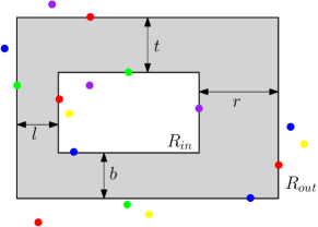
Figure 2: A RBRA with outer and inner rectangles $R_{\mathrm{out}}$ and $R_{\mathrm{in}}$ whose top-, bottom-, left-, right-widths are $t$, $b$, $l$, and $r$, respectively.

A circular annulus $\mathcal{A}$  is the region between two concentric disks $C_{\mathrm{out}}$ (outer disk) and $C_{\mathrm{in}}$ (inner disk) where $C_{\mathrm{in}}\subseteq C_{\mathrm{out}}$. The width of a circular annulus $\mathcal{A}$  is defined to be the difference of the radii of its outer and inner disks (see Figure 1(b)).

An annulus $\mathcal{A}$ is said to be rainbow-bisecting empty if it does not contain any point of $P$ in its interior and divides $P$ into two non-empty subsets such that each subset is a rainbow. One subset of $P$ lies within or on the boundary of the inner square/rectangle/disk of $\mathcal{A}$ and the other subset of $P$ lies outside or on the boundary of the outer square/rectangle/disk of $\mathcal{A}$. We now refer to an axis-parallel square (resp. rectangle) as square (resp. rectangle) for simplicity. Any rainbow-bisecting empty square annulus, rainbow-bisecting empty rectangular annulus and rainbow-bisecting empty circular annulus are denoted by RBSA, RBRA and RBCA, respectively.

3 Maximum-Width Rainbow-Bisecting Empty Square Annulus

In this section, we compute a maximum-width RBSA from a given point set $P$ on $\mathbb{R}^{2}$.

Lemma 1

There is a maximum-width RBSA with the outer square $S_{\mathrm{out}}$ and the inner square $S_{\mathrm{in}}$ such that a pair of sides with the same relative position in $S_{\mathrm{out}}$ and $S_{\mathrm{in}}$ each contains a point of $P$, and one of the following three conditions is satisfied.

• C₁: The remaining sides of $S_{\mathrm{out}}$ and $S_{\mathrm{in}}$ are at infinity (Figure 3(a)).

• C₂: For the side of $S_{\mathrm{out}}$ containing a point of $P$, one of two adjacent sides of $S_{\mathrm{out}}$ contains a point of $P$. The remaining sides of $S_{\mathrm{out}}$ are at infinity, and the corresponding sides of $S_{\mathrm{in}}$ are also at infinity (Figure 3(b)).

• C₃: For the side of $S_{\mathrm{out}}$ containing a point of $P$, the opposite side of $S_{\mathrm{out}}$ contains a point of $P$ (Figure 3(c)).

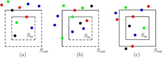
Figure 3: Three possible configurations of a maximum-width RBSA. The dashed sides represent the sides at infinity. (a) C₁ Configuration (b) C₂ Configuration (c) C₃ Configuration

Proof.  We start by proving the fact that outer and inner squares of a maximum-width $RBSA$ each contains a point of $P$ on their boundaries. For a contradiction, we assume that there is no point on the boundaries of the outer square $S_{\mathrm{out}}$ and the inner square $S_{\mathrm{in}}$ of a maximum-width RBSA, $\mathcal{A}$. Then, we can shrink $S_{\mathrm{in}}$ until the boundary of $S_{\mathrm{in}}$ hits a point in $P$, while keeping the center of $\mathcal{A}$ fixed. In this process no point goes outside from the inside of $S_{\mathrm{in}}$, so $\mathcal{A}$ remains empty. But the width of $\mathcal{A}$ increases which contradicts our assumption. Similarly, we can increase the width of $\mathcal{A}$ by extending $S_{\mathrm{out}}$ while keeping the center of $\mathcal{A}$ fixed, a contradiction. So there must be at least one point of $P$ lying on the boundary of $S_{\mathrm{in}}$ and on the boundary of $S_{\mathrm{out}}$.

Suppose that the sides of $S_{\mathrm{in}}$ and $S_{\mathrm{out}}$ that contain the points of $P$ have different relative positions in $S_{\mathrm{in}}$ and $S_{\mathrm{out}}$. Then, we can always get a RBSA with larger width by transforming $S_{\mathrm{in}}$ and $S_{\mathrm{out}}$ as in Figure 4. Therefore, the sides of $S_{\mathrm{in}}$ and $S_{\mathrm{out}}$ that contain the points of $P$ have the same relative position. Without loss of generality, we assume that both top sides of $S_{\mathrm{in}}$ and $S_{\mathrm{out}}$ contain the points of $P$.

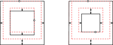
Figure 4: An example of transformation of inner and outer squares of a RBSA (red dashed) to get another RBSA (black filled) with larger width.

Next, we enlarge $S_{\mathrm{in}}$ and $S_{\mathrm{out}}$. During the process, the top sides of $S_{\mathrm{in}}$ and $S_{\mathrm{out}}$ keep the points of $P$ on the sides, and the width of $\mathcal{A}$ is fixed. The enlarging process will be finished when $S_{\mathrm{out}}$ encounters a point of $P$. If there is no such a point, then $\mathcal{A}$ belongs to C₁ configuration. If the enlarging process is finished with a point of $P$ on the bottom side of $S_{\mathrm{out}}$, then $\mathcal{A}$ belongs to C₃ configuration. If the enlarging process is finished with a point of $P$ on the left (resp. right) side of $S_{\mathrm{out}}$, we can continue the enlarging process with the bottom and the right (resp. left) sides of $S_{\mathrm{in}}$ and $S_{\mathrm{out}}$. If the enlarging process is finished with another point of $P$, then $\mathcal{A}$ belongs to C₃ configuration. If there is no such a point, then $\mathcal{A}$ belongs to C₂ configuration.

   

Thus to find a maximum-width RBSA from a given point set $P$, we solve the above three configurations and propose different algorithms for handling each of them. As a part of preprocessing, we sort the points in $P$ using their $x$- and $y$-coordinates, respectively.

Note that any RBSA belonging to configuration C₁ maps to an empty strip such that regions on both side of the strip are rainbow. We call such RBSA a rainbow-bisecting empty strip, RBES.

Lemma 2

A maximum-width RBES of a sorted set of points can be computed in $O(n)$ time using $O(n)$ space.

Now we discuss the solution technique for C₂ configuration. Observe solving this configuration corresponds to the problem of finding a widest rainbow-bisecting empty axis-parallel L-shaped corridor (RBLC). A RBLC is an axis-parallel empty L-shaped corridor which partitions the input point set $P$ into two non-empty rainbow subsets. Note that one can solve the problem by constructing $n^{2}$ grid points for given $n$ points and have the following trivial result.

Remark 1

Given a set of $n$ points in the plane, each colored with one of the given $k$ colors, a maximum-width RBLC can be computed in $O(n^{3})$ time using $O(n)$ space.

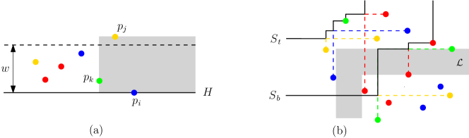
Figure 5: (a) The horizontal part of $\mathcal{L}$ should be contained in the gray region bounded by $p_{i}$, $p_{j}$, and $p_{k}$. (b) Two corners of $\mathcal{L}$ should be contained in the region bounded above S_t and below S_b.

We design a non-trivial algorithm for computing a maximum-width RBLC. Without loss of generality, we only consider the case where the RBLC is pointing down and right, and its width is determined from the $y$-gap of two points in $P$ (Figure 3(b)). Observe that we can handle all other cases analogously. Let $P=\{p_{1},p_{2},\ldots,p_{n}\}$ be the given set of points, sorted in the ascending order of their $y$-coordinates, that is, $y(p_{1})\leq y(p_{2})\leq\cdots\leq y(p_{n})$. We imagine sweeping a horizontal line $H$ upwards over the plane. It starts from the position $y=y(p_{1})$ and gradually moves upwards until all points in $P$ are visited. When the line $H$ sweeps through a point $p_{i}\in P$, we decide the existence of a RBLC $\mathcal{L}$ such that the horizontal part of $\mathcal{L}$ is right above $H$, and its width is larger than the width of the widest RBLC found so far. To find such RBLC $\mathcal{L}$, we use the following queries. Let $Q_{a}$ be the set of points above $y(p_{i})$ and $Q_{b}$ be the set of remaining points $P\setminus Q_{a}$.

1. Boundary points query: Let $w$ be the width of the widest RBLC found so far. First, we find the lowest point $p_{j}$ in $Q_{a}$ such that the $y$-gap between $p_{i}$ and $p_{j}$ is larger than $w$. Then $y$-gap between $p_{i}$ and $p_{j}$ becomes the width of $\mathcal{L}$. Among the points whose $y$-coordinates are in between $y(p_{i})$ and $y(p_{j})$, we find the point $p_{k}$ with the largest $x$-coordinate. Observe that the horizontal part of $\mathcal{L}$ should be contained in the region bounded by $p_{i}$, $p_{j}$, and $p_{k}$ from below, above, and left, respectively (Figure 5(a)).

2. Rainbow range query: Let S_b and S_t are two staircase structures such that any empty axis-parallel L-shaped corridor whose two corners are lying in the region above S_b and below S_t is a RBLC (Figure 5(b)). After the boundary points query, we compute the intersection $\mathcal{I}_{t}$ (resp. $\mathcal{I}_{b}$) between the horizontal line $y=y(p_{j})$ and S_t (resp. $y=y(p_{i})$ and S_b). The left (resp. right) side of the vertical part of $\mathcal{L}$ should be on the right (resp. left) of the intersection.

3. Maximum $x$-gap query: After the rainbow range query, we find the maximum $x$-gap between two consecutive points of $Q_{b}$ in range $[\max(x(\mathcal{I}_{t}),x(p_{k})),x(\mathcal{I}_{b})]$, when the points of $Q_{b}$ are sorted with respect to the $x$-coordinates. If the maximum $x$-gap is larger than $y$-gap between $p_{i}$ and $p_{j}$, then $\mathcal{L}$ exists.

To answer the above queries we use the following data structures :

• The point $p_{j}$ can be found in $O(\log n)$ time without any additional data structure. Let $\mathcal{T}$ be a one dimensional range tree built on the $y$-coordinate values of the points in $P$. Also each node $v\in\mathcal{T}$ stores the point with the maximum $x$-coordinate value among the points in the canonical subset of $v$. The tree $\mathcal{T}$ can be constructed in $O(n)$ time using $O(n)$ space [10], and finding the points with the maximum $x$-coordinate values can be done in $O(n)$ time in total. Using this data structure, we can find the point $p_{k}$ in $O(\log n)$ time.

• The corners of S_b and S_t are maintained in two balanced binary search trees $\mathcal{T}_{b}$ and $\mathcal{T}_{t}$ built on their $y$-coordinate values, respectively. We compute S_b as follows, and S_t can be computed similarly. Let $c$ be a point at $(-\infty,-\infty)$, and consider the region $R_{c}$ which is the intersection between two half spaces $x\geq x(c)$ and $y\leq y(c)$. Now we move $c$ upward until $R_{c}$ becomes a rainbow set. Next, we move $c$ to the right while $R_{c}$ is a rainbow set. When $c$ is stopped, there should be a point $p$ on the left side of $R_{c}$, and we move $c$ upward again until $R_{c}$ meets a point $q$ such that $\alpha(p)=\alpha(q)$. Then, we move $c$ to the right again, while $R_{c}$ is a rainbow set. By repeating this process, we can get S_b from the trace of $c$.
  
  As $P$ is sorted with respect to the $y$-coordinates, the next point to be contained in $R_{c}$ (as $c$ moves upward) can be found in $O(1)$ time. When adding a new point to $R_{c}$, we spend $O(\log n)$ time to keep the points in $R_{c}$ sorted with respect to the $x$-coordinates. Then we can find the next point to be removed from $R_{c}$ (as $c$ moves to the right) in $O(\log n)$ time. In total, we can compute $\mathcal{T}_{b}$ that stores the corners of S_b in $O(n\log n)$ time using $O(n)$ space. From $\mathcal{T}_{b}$ and $\mathcal{T}_{t}$, rainbow range query can be answered in $O(\log n)$ time.

• Let $\mathcal{T}_{i}$ be a one dimensional range tree build on the $x$-coordinate values of the points in $Q_{b}$. Also each node $v\in\mathcal{T}_{i}$ stores the maximum $x$-gap of two consecutive points in the canonical subset of $v$. The structure $\mathcal{T}_{i}$ can be computed from $\mathcal{T}_{i-1}$ by adding new point $p_{i}$ in $O(\log n)$ time, and the size of $\mathcal{T}_{i}$ is bounded by $O(n)$ [10]. The maximum $x$-gap query for a given range can be answered in $O(\log n)$ time by comparing $O(\log n)$ values including every gap between two consecutive canonical subsets.

With the above data structures in hand, we have the following result.

Lemma 3

The existence of a RBLC $\mathcal{L}$ can be determined (during the sweeping process) in $O(\log n)$ time such that the horizontal part of $\mathcal{L}$ is right above the sweeping line and it’s width is larger than the width of the widest RBLC found so far.

Our algorithm uses the result of Lemma 3 to obtain a maximum-width RBLC from $P$.

Theorem 1

Given $n$ points in $\mathbb{R}^{2}$ where each one is colored with one of the $k$ colors, a maximum-width RBLC can be found in $O(n\log n)$ time using $O(n)$ space.

Proof.  The sweeping line $H$ starts from the position $y=y(p_{1})$ and gradually moves upwards. When the sweeping line $H$ passes through a point $p_{i}$, we determine the existence of a RBLC $\mathcal{L}$ such that the horizontal part of $\mathcal{L}$ is right above $H$ and its width is larger than the width of the widest RBLC found so far. We repeat this until there is no such RBLC, and move $H$ to $y=y(p_{i+1})$. The width of $\mathcal{L}$ is determined by the $y$-gap between two points $p_{i}$ and $p_{j}$ where $1\leq i<j\leq n$, and both indices $i$ and $j$ do not decrease during the sweeping process. Therefore, the number of RBLCs we find during the sweeping process is $O(n)$, and we can find a maximum-width RBLC in $O(n\log n)$ time using $O(n)$ space.    

Here we mention that our algorithm improves the time complexity for computing a widest empty axis parallel L corridor for a given set of $n$ points in plane from $O(n^{2}\log n)$ (Theorem 1 of [6]) to $O(n\log n)$.

C₃ configuration: Any RBSA here is defined by two input points on both two opposite sides of its outer square. Assume that each of the top and bottom sides of the outer square of a RBSA contain a point of $P$. We design an algorithm to compute a maximum-width RBSA with the the top and bottom sides of its outer square containing points $p_{i}$ and $p_{j}$, respectively, from all pairs of indices $(i,j)$ with $1\leq i<j-1<n$. We start this case with the following observation.

Observation 1

For fixed points $p_{i}$ and $p_{j}$ which define the bottom and top sides of the outer square $S$ respectively, the potential locations of the center of $S$ lie on the line $\ell$ such that $y(\ell)=(y(p_{i})+y(p_{j}))/2$ (Ref. Figure 6).

Note that the outer square of a potential candidate annulus for fixed points $p_{i}$ and $p_{j}$ lies inside a rectangle $R$ (Ref. Figure 6) such that $x$(left)$=\max\{x(p_{i}),x(p_{j})\}-2r$ and $x$(right)$=\min\{x(p_{i}),x(p_{j})\}+2r$, where $r=(y(p_{j})-y(p_{i}))/2$.

Figure 6: Centers of candidate outer squares in $R$ lie in the horizontal segment $[a,b]$ such that $a=(max(x(p_{i}),x(p_{j}))-r,y(\ell))$ and $b=min(x(p_{i}),x(p_{j}))+r,y(\ell))$, where $y(\ell)=(y(p_{i})+y(p_{j}))/2$ and $r=(y(p_{j})-y(p_{i}))/2$.

We maintain color counter vectors to maintain the number of points of each color present outside and inside the horizontal strip defined by points $p_{i}$ and $p_{j}$. Since the target annulus is a RBSA, therefore rectangle $R$ must be a rainbow rectangle. We only consider such rectangles.

For a fixed outer square $S(c)$ with center $c$ lies on $[a,b]\subset\ell$, we compute the radius of the inner square $S^{\prime}(c)$ by finding the farthest point from center $c$ lying inside $S(c)$. For this, we plot $L_{\infty}$ distances from $c$ to each point $p$ in $R$ along $[a,b]$. Bae et al. [6] showed that the upper envelope of the $L_{\infty}$ distances has $O(n)$ complexity and can be computed in $O(n)$ time. From the centers of the annuli obtained by mapping the breakpoints of the upper envelope, we identify those annuli which are RBSA. Finally our algorithm outputs the one with the largest width. Considering all choices of $p_{i}$ and $p_{j}$ and the above discussion leads to the following result.

Lemma 4

A maximum-width RBSA corresponding to C₃ configuration can be computed in $O(n^{3})$ time and $O(n)$ space.

Proof.  For a fixed $p_{i}$ and $p_{j}$, the centers of all possible empty annuli can be computed in $O(n^{3})$ time [6] and $O(n)$ space. In another linear scan we can find the RBSA with the maximum-width. The result follows by taking all values of $i$ and $j$.    

We conclude the section with the following theorem.

Theorem 2

Given $n$ points in $\mathbb{R}^{2}$ where each one is colored with one of the $k$ colors, a maximum-width RBSA can be computed in $O(n^{3})$ time using $O(n)$ space.

Proof.  A maximum-width RBSA results from any of the three configurations from Lemma 1. For C₁ configuration, the maximum one is reported in $O(n)$ time using $O(n)$ space from Lemma 2 if the points are already sorted. For C₂ configuration, we find a maximum-width RBLC in $O(n\log n)$ time using $O(n)$ space from Theorem 1. For C₃ configuration, we compute a maximum-width RBSA in $O(n^{3})$ time using $O(n)$ space from Lemma 4. Hence the statement followed.    

4 Maximum-Width Rainbow-Bisecting Empty Rectangular Annulus

In this section, we discuss an algorithm to compute a maximum-width rainbow-bisecting empty rectangular annulus amidst a given point set $P$ on $\mathbb{R}^{2}$. The following observation shows the existence of a maximum-width RBRA meeting certain conditions.

Observation 2

There exists a maximum-width RBRA $\mathcal{A}$ with outer rectangle $R_{out}$ and inner rectangle $R_{in}$ satisfying the following conditions: (1) Each side of $R_{out}$ contains a point of $P$ or lies at infinity; (2) Each side of $R_{in}$ contains a point of $P$.

Proof.  Consider any maximum-width RBRA $\mathcal{A}$, and assume that the boundary of $R_{out}$ does not contain any input point. We enlarge each side of $R_{out}$ till each of them contains a point of $P$ or they are at infinity. Similarly we shrink $R_{in}$ by pushing each side inwards until each side hits a point. Note that any two adjacent sides of $R_{in}$ can share a point at its corner. In this process the width of $\mathcal{A}$ is not decreased. By our construction, we create a new maximum-width RBRA from $\mathcal{A}$ that satisfies the conditions.    

From Observation 2, we can find a maximum-width RBRA by examining every rectangular annulus that satisfying the conditions in Observation 2. The outer rectangle $R_{out}$ of a rectangular annulus $A$ can be determined by at most $4$ points of $P$, and the inner rectangle $R_{in}$ of $A$ becomes the minimum rectangle that contains the points $P\cap R_{out}$. This results in a trivial algorithm.

Remark 2

For a given set of $n$ points $P$, where each point in $P$ is assigned a color from given $k$ colors, a maximum-width RBRA can be reported in $O(n^{5})$ time.

A RBRA is called RBRA with uniform width, or simply uniform RBRA, when it has all four widths (top, bottom, left and right) equal. The following observation shows that we can construct a maximum width RBRA with uniform width from any maximum width RBRA.

Observation 3

For any maximum-width RBRA, we can construct a maximum-width RBRA with uniform width satisfying the following characteristic: each side of its outer rectangle either contains a point of $P$ or lies at infinity, and at least one side of its inner rectangle contains a point of $P$.

Proof.  For a maximum-width RBRA $\mathcal{A}$, let $\mathcal{A}$^′ be a maximum-width RBRA that satisfies the conditions in Observation 2 created by transforming $\mathcal{A}$ according to the process in Observation 2. Let $R_{out}$ and $R_{in}$ be the outer and inner rectangles of $\mathcal{A}$^′, and $w$ be the width of $\mathcal{A}$^′. Therefore every side of $R_{out}$ contains at least one point of $P$ or lies at infinity. Now think that the width $w$ comes from the horizontal distance of left sides (left-width) of $\mathcal{A}$^′. We enlarge the remaining three sides of $R_{in}$ to form another rectangle $R^{\prime}_{in}$, where $R^{\prime}_{in}\subseteq R_{out}$, and all the four widths (top, bottom, left and right) of the new annulus, $\mathcal{A}$^′′, thus formed are equal. The width of $\mathcal{A}$^′′ is equal to $w$. Since $R_{in}\subseteq R^{\prime}_{in}$ and thus $\mathcal{A}$${}^{\prime\prime}\subseteq$$\mathcal{A}$^′, suggests $\mathcal{A}$^′′ is also a RBRA. See Figure 7 for an illustration.    

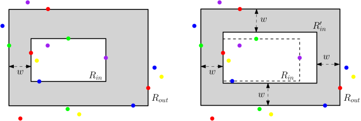
Figure 7: (left) A maximum-width RBRA of width $w$ (right) A left-anchored maximum-width RBRA with uniform width.

As introduced in Bae et al. [6], we call a rectangular annulus $\mathcal{A}$ top-anchored (or, bottom-anchorsed, left-anchored, right-anchored) if the following conditions are satisfied: (1) top (or, bottom, left, right, resp.) side of the outer rectangle of $\mathcal{A}$ contain a point of $P$ or lies at infinity; (2) top (or, bottom, left, right, resp.) side of the inner rectangle of $\mathcal{A}$ contains a point of $P$. A maximum-width RBRA with uniform width has the following property.

Observation 4

A maximum-width RBRA with uniform width can be either top-anchored, bottom-anchored, left-anchored or right-anchored (Figure 7(right)).

In a nutshell our problem boils down to the problem of computing an anchored and uniform maximum-width RBRA. Here, we only discuss the case where the RBRA is “top-anchored”. The other three cases can be similarly handled.

A brief outline of our algorithm that computes a top-anchored and uniform RBRA of maximum-width is as follows: Consider the given set of points $P=\{p_{1},p_{2},\ldots,p_{n}\}$, sorted in decreasing order of their $y$-coordinates and $X$ be an array of size $k$ where $X[i]$ indicates the number of points of color $i$. Consider any top-anchored and uniform RBRA $\mathcal{A}$ that satisfies the condition of Observation 3. Let $p_{i}\in P$ be the point lying on the top side of the outer rectangle of $\mathcal{A}$. From the assumption on $\mathcal{A}$, either the bottom side of the outer rectangle of $\mathcal{A}$ is at infinity or there is another point $p_{j}\in P$ for $i<j\leq n$ on it. Since $\mathcal{A}$ is top-anchored, there is a third point $p_{k}\in P$ on the top side of the inner rectangle of $\mathcal{A}$. Note that the width of $\mathcal{A}$ is determined by the $y$-difference of $p_{i}$ and $p_{k}$, that is, $y(p_{i})-y(p_{k})$. Thus, the maximum width for top-anchored annuli is one among $O(n^{2})$ values $\{y(p_{i})-y(p_{k})\mid 1\leq i\leq k\leq n\}$.
Initially we study the case where two points $p_{i}$ and $p_{j}$ on the top and bottom sides are fixed, and then discuss the situation where only a point $p_{i}$ on the top side is fixed. We discuss a decision algorithm when two points on the top and bottom sides of the outer rectangle are fixed, and use it as a sub-routine for solving the other case.

4.1 Decision problem for fixed top and bottom sides

Here we discuss a decision algorithm when two points $p_{i}$ and $p_{j}$ are fixed on the top and bottom sides of outer rectangle of the RBRA, where $2\leq i+1<j\leq n$. To represent the case when the bottom side of the outer rectangle lies at infinity, we use ${j}=\infty$. The decision problem $DP_{ij}(w)$ is defined as follows:

Given: A positive real $w>0$, two indices $i$ and $j$ where $2\leq i+1<j\leq n$, or $j=\infty$. Task: Decides the existence of a RBRA of width at least $w$ and whose outer rectangle contains $p_{i}$ and $p_{j}$ on its top and bottom sides, respectively.

The following observation holds on $DP_{ij}(w)$.

Observation 5

If $DP_{ij}(w)$ is TRUE, then $DP_{ij}(w^{\prime})$ is TRUE for any $w^{\prime}\leq w$. On the other hand, if $DP_{ij}(w)$ is FALSE, then $DP_{ij}(w^{\prime})$ is FALSE for any $w^{\prime}\geq w$.

To compute $DP_{ij}(w)$, we consider the set $P_{ij}:=\{p_{i+1},\ldots,p_{j-1}\}$ containing points between $y(p_{i})$ and $y(p_{j})$ where $2\leq i+1<j\leq n$, and $P_{i\infty}:=\{p_{i+1},\ldots,p_{n}\}$. The decision algorithm perform the $y$-range $x$-neighbor query operation [6] on points of $P_{ij}$ to evaluate $DP_{ij}(w)$.
We present Algorithm 1 to answer the decision problem $DP_{ij}(w)$. The algorithm calls the $y$-range $x$-neighbor query twice. Also, if the algorithm decides that $DP_{ij}(w)$ is TRUE, then it also returns a corresponding RBRA, that is, a RBRA with uniform width $w$ such that $p_{i}$ and $p_{j}$ on the top and bottom sides of its outer rectangle.

Input: A positive real $w>0$, two indices $i$ and $j$ where $2\leq i+1<j\leq n$, or $j=\infty$.

Output: $DP_{ij}(w)$ and if $DP_{ij}(w)$ is TRUE then the algorithm outputs a RBRA with uniform width $w$ having $p_{i}$ and $p_{j}$ lying on the top and bottom sides of its outer rectangle, respectively.

1

2if $y(p_{i})-y(p_{j})<2w$ then

3      Return FALSE.

4Search the rightmost and the leftmost points from the sets $P_{ij}\cap[-\infty,x(p_{i})]\times[y(p_{i})-w,y(p_{i})]$ and $P_{ij}\cap[x(p_{i}),+\infty]\times[y(p_{i})-w,y(p_{i})]$ respectively. Let these two points be $l_{1}$ and $r_{1}$ respectively.

5

6Search the rightmost and the leftmost points from the sets $P_{ij}\cap[-\infty,x(p_{j})]\times[y(p_{j}),y(p_{j})+w]$ and $P_{ij}\cap[x(p_{j}),+\infty]\times[y(p_{j}),y(p_{j})+w]$ respectively. Let these two points be $l_{2}$ and $r_{2}$ respectively.

7

8Let $p_{l}$ be the rightmost one in $\{l_{1},l_{2}\}$ and $p_{r}$ be the leftmost one in $\{r_{1},r_{2}\}$.

9

10if $\min\{x(p_{i}),x(p_{j})\}<x(p_{l})<\max\{x(p_{i}),x(p_{j})\}$ or $\min\{x(p_{i}),x(p_{j})\}<x(p_{r})<\max\{x(p_{i}),x(p_{j})\}$ then

11      Return FALSE.

12Search all the horizontal gaps of length at least $w$ from the points lying in the range $(x(p_{l}),\min\{x(p_{i}),x(p_{j})\}+w)$. Let $\mathcal{L}$ denote the set of such gaps. // Boundary points are included in the search range.

13

14Search all the horizontal gaps of length at least $w$ from the points lying in the range $(\max\{x(p_{i}),x(p_{j})\}-w,x(p_{r}))$. Let $\mathcal{R}$ denote the set of such gaps. // Boundary points are included in the search range.

15

16if $\mathcal{L}\neq\emptyset$ and $\mathcal{R}\neq\emptyset$ then

17      Start with the leftmost horizontal gap (say, $g_{l}:=x(l_{a})-x(l_{b})$) from set $\mathcal{L}$. Maintain the number of points of each color on the left side of $g_{l}$. From $x(l_{a})$ start moving forward until a point say, $p_{in}$ comes such that the points from $x(l_{a})$ to $x(p_{in})$ forms a rainbow region. Move forward from $p_{in}$ until a point say, $p_{out}$ is reached such that if moved further the region outside the region bounded by $x(l_{b})$, $x(p_{out})$, $y(p_{i})$ and $y(p_{j})$ is not rainbow. Search a $w$ width horizontal gap between $x(p_{in})$ and $x(p_{out})$ and check if it lies within $(\max\{x(p_{i}),x(p_{j})\}-w,x(p_{r}))$. Repeat the procedure for all the gaps in $\mathcal{L}$ until such a gap is found that defines the right sides of RBRA. Return TRUE if such gap exists, and RBRA of uniform width $w$. Otherwise Return FALSE.

18else

19      Return FALSE.

Algorithm 1 Decision algorithm

Next, we prove the correctness of Algorithm 1.

Lemma 5

Algorithm 1 correctly computes $DP_{ij}(w)$ for any given $w>0$ in $O(n)$ time.

Proof.  The time complexity of Algorithm 1 depends on the search queries given in line numbers 3, 4, 8, 9 and 11. In line 3 and 4, the search queries can be done in $O(\log n)$ time [6]. Since the points are maintained in sorted order, the operations in lines 8, 9 and 11 can be done in $O(n)$ time. For any horizontal gap of length at least $w$ from $\mathcal{L}$ that defines the left sides of the RBRA we search for the corresponding right sides such that rainbow property is satisfied and right sides are in $\mathcal{R}$. In line 11, we start searching for points $p_{in}$ and $p_{out}$ for the leftmost gap $g_{l}$ in set $\mathcal{L}$. At the same time we maintain a count on the number of points of each color we seen so far, starting from $x(l_{a})$. At $x(p_{in})$ we have exactly $k$ colors present. Similarly at $x(p_{out})$ we have exactly $k$ colors present outside the region (including the boundaries) bounded by lines $x(l_{b})$, $x(p_{out})$, $y(p_{i})$ and $y(p_{j})$ from left, right, top and bottom respectively. This operation is repeated for all gaps in $\mathcal{L}$ and every time it advances to the next gap, the points $p_{in}$ and $p_{out}$ move forward from their previous positions. During the repetition, if Algorithm 1 finds a RBRA with uniform width $w$, it returns TRUE and the RBRA.    

4.2 Optimization Algorithm

We now move to the case where we fix only a point $p_{i}\in P$ that defines the top side of the outer rectangle and compute a top-anchored and uniform RBRA $\mathcal{A}$^′ of maximum-width for the point set $P$.

If $p_{i}$ lies on the top side of the outer rectangle of a top-anchored and uniform RBRA $\mathcal{A}$, then the width of $\mathcal{A}$ should be in the set $W=\{y(p_{i})-y(p_{k})\mid i<k\leq n\}$. Thus, we can find $\mathcal{A}$^′ by solving $DP_{ij}(w)$ with Algorithm 1 for every $i+1<j$ and $w\in W$. There are a total of $O(n^{2})$ of $DP_{ij}(w)$ to solve, but we can find $\mathcal{A}$^′ by solving only $O(n)$ of them.

Lemma 6

For a point $p_{i}\in P$, a top-anchored and uniform RBRA $\mathcal{A}$of maximum-width such that $p_{i}$ lies on the top side of the outer rectangle of $\mathcal{A}$ can be computed in $O(n^{2})$ time.

Proof.  For a fixed $p_{i}$, there are $O(n)$ candidate widths $w$ of the annulus and $O(n)$ candidate points $p_{j}$ which lie on the bottom side of the outer rectangle. We need to find the maximum width $w^{*}$ such that $DP_{ij^{*}}(w^{*})$ is TRUE for an index $j^{*}$ with $i+2<j^{*}$.

Let index $j=i+2$ and width $w=y(p_{i})-y(p_{i+1})$ be the smallest possible values among the candidates, and solve $DP_{ij}(w)$ using Algorithm 1. If $DP_{ij}(w)$ is TRUE, then we set $w$ as the next smallest candidate width $w=y(p_{i})-y(p_{i+2})$ and solve $DP_{ij}(w)$ again. We repeat this process until $DP_{ij}(w)$ becomes FALSE. From Observation 5, $DP_{ij}(w^{\prime})$ is FALSE for all $w^{\prime}>w$, so we don’t need to solve $DP_{ij}(w^{\prime})$ for $w^{\prime}>w$. Thus we increase $j$ by one, and repeat the process to find the maximum width such that $DP_{ij}(w)$ is TRUE. We repeat the entire process until $j=\infty$ or $w=y(p_{i})-y(p_{n})$, and we can find the maximum width $w^{\prime}$ during the process.

The suggested process only increase both $w$ and $j$, so we call Algorithm 1 at most $O(n)$ times. Therefore it takes $O(n^{2})$ time to report a top-anchored and uniform RBRA of maximum-width for $p_{i}$.    

We have $n$ possible choices for $p_{i}$, so we can find a top-anchored and uniform RBRA of maximum-width in $O(n^{3})$ time, and the other three cases (bottom-anchored, left-anchored, or right-anchored) of the maximum-width RBRA are handled similarly. We conclude the section with the following result.

Theorem 3

Given a set $P$ of $n$ points in the plane where each one is assigned a color from given $k$ colors, a maximum-width RBRA with respect to $P$ can be computed in $O(n^{3})$ time and $O(n)$ space.

4.3 An Improved Approach

In Section 4.1, we present a $O(n)$ time decision algorithm to compute a maximum-width RBRA, where the top and bottom sides of its outer rectangle pass through two fixed points. Here we show that Algorithm 1 can be implemented in $O(k^{2}\log n)$ time.
Let $a$ be any $w$-gap from the set $\mathcal{L}$ (described in Step 8 of Algorithm 1). We are interested in the leftmost $w$-gap $b$ from the set $\mathcal{R}$ such that the corresponding inner rectangle is rainbow and the number of points outside of the annulus is maximum. Note that the inner rectangle defined by $a$ and any $w$-gap $b^{\prime}$ in $\mathcal{R}$ to the right of $b$ is rainbow, while the number of points is less lying outside of the outer rectangle of the annulus. On the other hand, if we find the rightmost $w$-gap $a^{\prime}$ in $\mathcal{L}$ such that the corresponding inner rectangle defined by $a^{\prime}$ and $b$ is rainbow, then either $a=a^{\prime}$ or $a^{\prime}$ lies to the right of $a$. Note that in the latter case we can ignore the $w$-gap $a$, since the annulus defined by $w$-gaps ($a^{\prime},b$) is better than that defined by ($a,b$) in the sense of the number of points lying outside the outer rectangle of the annulus.

4.3.1 Minimal Rainbow Intervals

Consider the set $L$ of points $P_{ij}\cap[x(p_{l}),\min\{x(p_{i}),x(p_{j})\}+w]\times[y(p_{j}),y(p_{i})]$. Then, $\mathcal{L}$ denotes the set of $w$-gaps in $x$-coordinates of $L$. Similarly $R$ be the set of points $P_{ij}\cap[\max\{x(p_{i}),x(p_{j})\}-w,x(p_{r})]\times[y(p_{j}),y(p_{i})]$. For our purpose we only consider the $x$-coordinates of the points in $P_{ij}$ and assume that the points are projected down on the $x$-axis.
Let $a$ be any point in $L$. We define $r(a)$ as the leftmost point in $R$ such that $P_{ij}\cap[a,r(a)]$ is rainbow. Similarly for any point $b$ in $R$, define $l(b)$ as the rightmost point in $L$ such that $P_{ij}\cap[l(b),b]$ is rainbow. Note that as $a$ moves to the right, $r(a)$ either moves to the right or stays at the same position. Similarly it holds for $l(b)$. We call an interval $[a,b]$ as minimal rainbow interval with $a\in L$ and $b\in R$, if $b=r(a)=r(l(b))$ and $a=l(b)=l(r(a))$. In the following we give some properties of minimal rainbow interval.
Recall that $\alpha(p)$ denotes the color of a point $p$, and let $c_{[Q]}$ denotes the number of points of color $c$ in a point set $Q$.

• If $[a,b]$ is a minimal rainbow interval, then either $\alpha(a)_{[a,b]}=1$ or $a$ is the rightmost point in $L$; $\alpha(b)_{[a,b]}=1$ or $b$ is the leftmost point in $R$. In other words, $a$ is the only point of that particular color in $[a,b]$ unless $a$ is the rightmost point in $L$, and so is $b$.

• No two minimal rainbow intervals are nested, and any two minimal rainbow intervals overlap.

• There cannot be two minimal rainbow intervals $[a_{1},b_{1}]$ and $[a_{2},b_{2}]$ such that $a_{1}$ and $a_{2}$ are in the same color, or $b_{1}$ and $b_{2}$ are in the same color. Also from (ii) we can order all minimal rainbow intervals from left to right, $[a_{1},b_{1}]$, $[a_{2},b_{2}]$,…, $[a_{m},b_{m}]$ with $a_{1}<a_{2}<\ldots<a_{m}$ and $b_{1}<b_{2}<\ldots<b_{m}$. Since the colors of $a_{1},a_{2}\ldots,a_{m}$ (resp. $b_{1},b_{2}\ldots,b_{m}$) must be all distinct, implies that $m$ can be at most $k$.

We are interested in the $w$-gaps that are generated in between minimal rainbow intervals. In the following lemma we present a bound on the number of “relevant” $w$-gaps. More specifically, for a given $p_{i}$ and $p_{j}$, a $w$-gap is relevant if $w\in\mathcal{L}$ or $w\in\mathcal{R}$.

Lemma 7

The number of relevant $w$-gaps is at most $O(k)$.

Proof.  Consider any $w$-gap $A$ in $\mathcal{L}$. Also assume that $A$ is between the left endpoints of minimal rainbow intervals $[a_{1},b_{1}]$ and $[a_{2},b_{2}]$, i.e., $A$ lies between $a_{1}$ and $a_{2}$. Therefore, the leftmost $w$-gap $b$ in $\mathcal{R}$ such that the inner rectangle defined by ($A,B$) is rainbow must lies somewhere to the right of $b_{2}$. If there lies another $w$-gap $A^{\prime}$ between $a_{1}$ and $a_{2}$ that is to the right of $A$, we can simply ignore $A$. In a nutshell, we consider only the rightmost $w$-gap to the left of the left endpoint of each minimal rainbow interval and the leftmost $w$-gap to the right of the right endpoint of each minimal rainbow interval. Hence, the number of these “relevant” $w$-gaps is at most $2k$.    

4.3.2 Modified Decision Algorithm

Here we discuss the new decision problem $DA_{new}$ that computes $DP_{ij}(w)$. $DA_{new}$ have exactly same lines 1 to 7 as stated in Algorithm 1. The new algorithm then computes all possible minimal rainbow intervals in between $y(p_{i})$ and $y(p_{j})$ as follows. Consider the points in $L$. For each point $a$ in $L$, we compute $r(a)$ as follows. For each color $c\in k$, compute the closest point in $P_{ij}$ of color $c$ to the right of $a$ and then find the farthest point $b$ from them. If $b$ is in $R$, then $r(a)=b$; otherwise $r(a)$ is the leftmost point in $R$ by definition. Similarly, for each point $b$ in $R$, we compute $l(b)$.

To compute all minimal rainbow intervals, first we start with the leftmost point $a\in L$, compute $b=r(a)$, and then compute $l(b)$. Therefore, $[l(b),b]=[a_{1},b_{1}]$ denotes the first minimal rainbow interval. If $a_{1}$ is the rightmost point in $L$, then $[a_{1},b_{1}]$ is the only minimal rainbow interval. Otherwise, we search for the second minimal rainbow interval $[a_{2},b_{2}]$. Since there is no point of color $\alpha(a_{1})$ in $[a_{1},b_{1}]$ other than $a_{1}$, therefore $\alpha(b_{2})=\alpha(a_{1})$. So, $b_{2}$ can be easily found by finding the closest point of color $\alpha(a_{1})$ in $P_{ij}$ to the right of $b_{1}$. Also then, $a_{2}=l(b_{2})$. The above process continues until we reach the rightmost point in $L$.

Consider any minimal rainbow interval $[a,b]$. We store $k$ counters for $[a,b]$. Let $C([a,b])=\#\_1([a,b]),\#\_2([a,b]),\ldots,\#\_k([a,b])$ be the color counter vector, consisting of the number of points in $P_{ij}$ of each color. For each minimal rainbow interval, we store its color counter vector.
For each $[a,b]\in[a_{1},b_{1}]$, $[a_{2},b_{2}]$,…, $[a_{m},b_{m}]$, we repeat the following steps:

$(i)$ First we compute the rightmost $w$-gap $A$ to the left of $a$, if any. Find the leftmost $w$-gap $B$ to the right of $b$, if any.
$(ii)$ Compute the color counter vector of the region between $A$ and $a$ and of the region between $b$ and $B$. Also compute the counter $C([A,B])$ for points between $A$ and $B$.
$(iii)$ From $C([A,B])$, the number of points of each color that lie outside the annulus can be found.

After the completion of the above steps if there exixts a RBRA of $w$-width, $DA_{new}$ reports it. In order to perform the above operations efficiently the following data structures are being used.

• Consider the 1-dimensional range tree $\mathcal{X}_{ij}(c)$, where $c\in[k]$, for the $x$-coordinates of points in $P_{ij}$ for counting for color $c$. Also at each node $v$ of the tree, we store $size(v)$, the number of leaves descended from $v$. The data structure $\mathcal{X}_{ij}(c)$ can be constructed using storage $O(|P_{ij}(c)|)$ [10], where $|P_{ij}(c)|$ represents the number of points of color $c$ in $P_{ij}$. We maintain $O(k)$ such 1D range trees.

• We preprocess the points of $P_{ij}$ into a 2D range tree (with fractional cascading) $\mathcal{T}_{ij}$ as follows: Let $x_{1}<x_{2}<\ldots$, be the $x$-coordinates of points in $P_{ij}$ in sorted order. Here we map each $x_{i}$ into a 2D point ($x_{i}$, $x_{i+1}-x_{i}$). We construct $\mathcal{T}_{ij}$ on these 2D points. $\mathcal{T}_{ij}$ can be constructed using storage $O(|P_{ij}|\log|P_{ij}|)$ [10].

With the above data structures in hand we can compute all minimal rainbow intervals and perform the mentioned operations on them as follows:

• For any point $a\in L$ (resp. for each point $b$ in $R$), we find $r(a)$ (resp. $l(b)$) in $O(k\log n)$ time from $k$ given 1D range trees. Thus in $O(k\log n)$ time we compute a minimal rainbow interval.

• To compute the leftmost $w$-gap to the right of a minimum rainbow interval $[a,b]$, more specifically the leftmost $w$-gap to the right of $b$, we use a 3-sided range query defined by the region $R=[x(b),min(x(r_{1}),x(r_{2}))-w]\times[w,\infty]$, where $r_{1}$ is the leftmost point from the region $[x(p_{i}),\infty]\times[y(p_{i})-w,y(p_{i})]$, and $r_{2}$ is the leftmost point from the region $[x(p_{j}),\infty]\times[y(p_{j}),y(p_{j})+w]$. Here we find the leftmost point from region $R$. From $\mathcal{T}_{ij}$ we can find the leftmost point in $R$ in $O(\log n)$ time. Any $w$-gap corresponds to a point in $R$ and can be used to construct an empty annulus of width $w$.

• For any rectangular region $R$, the color counter vector $C(R)$ of $R$ can be computed in $O(k\log n)$ time from $k$ given 1D range trees.

  Similarly, the color counter vector of the region between $A$ and $a$ (resp. between $b$ and $B$) and $C([A,B])$ (mentioned in step $(ii)$) can be computed in $O(k\log n)$ time.

• Using $C([A,B])$ we can find the number of points outside the empty annulus in $O(k)$ time.

Lemma 8

$DA_{new}$ computes $DP_{ij}(w)$ for any given $w>0$ in $O(k^{2}\log n)$ time using $O(n\log n)$ space.

Proof.  $DA_{new}$ takes $O(\log n)$ time [6] to compute lines 3 and 4. After getting TRUE in line 7 of Algorithm 1, $DA_{new}$ computes all minimal rainbow intervals. Since there are $O(k)$ minimal rainbow intervals in total, it takes $O(k^{2}\log n)$ time. For any minimal rainbow interval $DA_{new}$ construct a $w$-width RBRA if exists in $O(k\log n)$ time and $O(n\log n)$ space using the data structures mentioned above. Considering all minimal rainbow intervals the total running time is $O(k^{2}\log n)$.    

Now we discuss how to report a maximum-width top-anchored RBRA when a point $p_{i}\in P$ is fixed on the top side of outer rectangle of RBRA. Assume any point $p_{i}\in P$ lies on the top side of outer rectangle of RBRA. For a fixed $p_{i}$, we consider the widths that lies in the set $W_{i}:=\{y(p_{i})-y(p_{k})\mid i\leq k\leq n\}$ and report the maximum among them. The optimization algorithm is described in section 4.2. Having $p_{i}$ fixed, consider all possible values of $j=i+2,\ldots,n$ and also $j=\infty$. As $j$ increases, more points are included in $P_{ij}$ and therefore we update the structures by inserting a point in each of them. Since we use $O(k)$ tree data structures, the updates can be done in $O(k\log n)$ time. Therefore in this case we can report a maximum width top-anchored RBRA in $O(k^{2}n\log n)$ time. Considering all values of $p_{i}$, along with the above discussion we have the following result.

Theorem 4

For a given set of $n$ points in the plane where each point is assigned a color from given $k$ colors, a maximum-width top-anchored RBRA can be computed in $O(k^{2}n^{2}\log n)$ time and $O(n\log n)$ space.

5 Maximum-width Rainbow-Bisecting Empty Circular Annulus

In this section, we compute a maximum-width RBCA from a given point set $P$ on $\mathbb{R}^{2}$. Here we assume no four input points are concyclic.

Lemma 9

A maximum-width RBCA $\mathcal{A}$ is defined by four points from $P$ resulting one of the following potential configurations-$(i)$ Type $1$ (resp. Type $2)$ - $C_{\mathrm{out}}$ $($resp. $C_{\mathrm{in}})$ has three points of $P$ and $C_{\mathrm{in}}$ $($resp. $C_{\mathrm{out}})$ contains one point of $P$ and $(ii)$ Type $3$ - Each of $C_{\mathrm{in}}$ and $C_{\mathrm{out}}$ are defined by two points of $P$.

Proof.  For a contradiction, we assume that a maximum-width RBCA $\mathcal{A}$ is defined by three points. First, we deal with the case such that $C_{\mathrm{in}}$ has two points $p_{1}$ and $p_{2}$ and $C_{\mathrm{out}}$ has a point $p_{3}$ of $P$. Since $C_{\mathrm{in}}$ has two points $p_{1}$ and $p_{2}$, the center $c$ of the annulus $\mathcal{A}$ will lie on their perpendicular bisector, say $L$. Let $s$ be the center of the disk having points $p_{1}$, $p_{2}$ and $p_{3}$ on its boundary. The $width$ of annulus $\mathcal{A}$ will increase if we move the center $c$ in a direction away from $s$ along $L$ while $\mathcal{A}$ remains empty and both the regions inside and outside $C_{\mathrm{in}}$ and $C_{\mathrm{out}}$ are rainbow, respectively. Thus $\mathcal{A}$ cannot be a maximum-width $RBCA$.
The remaining cases can be treated similarly, so we prove that a maximum-width RBCA must be defined by four input points.     Adopting the technique of D.Báñez et al. [12], transform the points $\in P$ from $\mathbb{R}^{2}$ to $\mathbb{R}^{3}$ using paraboloid lifting (Figure 8) resulting the problem of computing the largest empty circular annulus problem in $\mathbb{R}^{2}$ being mapped to the largest empty slab problem (LESP) in $\mathbb{R}^{3}$.

Largest Empty Slab Problem: (LESP) Given: A set $S$ of $n$ points in $\mathbb{R}^{3}$ Task: Find a widest empty slab where a slab through $S$ is the open region of $\mathbb{R}^{3}$ that is bounded by $2$ parallel planes intersecting the convex hull of $S$. The width of the slab is the distance between the bounding planes.

Figure 8: Paraboloid transformation of the input points. Left side maps right side.

A candidate annulus (in $\mathbb{R}^{2}$) of Type $1$ (or $2$) $\&$ Type $3$ is being mapped (in $\mathbb{R}^{3}$) to empty slabs of Type $C_{\mathrm{31}}$ and $C_{\mathrm{22}}$ respectively (Figure 9). Finally, the optimal solution is obtained by tracking the slabs of Type $C_{\mathrm{31}}$ and $C_{\mathrm{22}}$ which span $k$ colors on both sides of it.

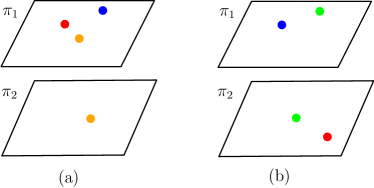
Figure 9: (a) A $C_{\mathrm{31}}$ empty slab defined by 2 parallel planes $\pi_{1}$ and $\pi_{2}$. (b) A $C_{\mathrm{22}}$ empty slab.

Generate candidate empty slabs of Types $C_{31}$, $C_{22}$ using topological sweep [4, 14] on the arrangement $\mathcal{H}$ of dual planes (each plane has a color) corresponding to the points in primal. During the sweep we maintain a count on the number of planes of each color in $[k]$ present above and below for each edge of the current planar cut of each plane. Once the initial planar cut for plane $k^{\prime}\in\mathcal{H}$ is determined, we initialize arrays namely $UP_{k^{\prime}}[1:k]$, $LOW_{k^{\prime}}[1:k]$ and $CO_{k^{\prime}}[1:n-1]$ following sequence of edges in $N_{k^{\prime}}[1:n-1]$, where $N_{k^{\prime}}[1:n-1]$ is a list of pairs of indices indicating the lines delimiting each edge of the current planar cut for plane $k^{\prime}$. The array $CO_{k^{\prime}}[i]=(a,b)$, indicates the number of colored planes above and below each edge of $N_{k^{\prime}}[i]$ of current planar cut for $k^{\prime}$ where $UP_{k^{\prime}}$ and $LOW_{k^{\prime}}$ help to initialize $CO_{k^{\prime}}$. We get each $CO_{k^{\prime}}$ in $O(n)$ time. As the sweep performs an elementary step, the incoming edges are swapped at the corresponding vertex in each planar cut and $CO_{k^{\prime}}$ is updated following new $N_{k^{\prime}}$ in $O(1)$ time. The above discussion along with lemma $4$ [12] leads to the following result.

Theorem 5

Given a set of $n$ points in $\mathbb{R}^{2}$, each one is colored with one of the $k$ colors, the maximum-width RBCA problem can be solved in $O(n^{3})$ time and $O(n^{2})$ space.

We extend the above idea to compute a maximum-width $RBCA$ whose center lies on a given line $L$ in the plane. We have the following lemma.

Lemma 10

A maximum-width RBCA $A$ whose center lies on a given line $L$ is defined by three points of $P$ where $C_{\mathrm{in}}$ (resp. $C_{\mathrm{out}}$) contains two points of $P$ and $C_{\mathrm{out}}$ (resp. $C_{\mathrm{in}}$) contains one point of $P$.

Proof.  Similar as described in lemma 9.     We conclude this section with the following corollary.

Corollary 1

A maximum-width RBCA $A$ whose center lies on a given query line $L$ in $\mathbb{R}^{2}$ can be computed in $O(n^{2})$ time and space.

6 Conclusion

In this paper, we have dealt with the problem of computing a maximum-width rainbow-bisecting empty annulus for three type of basic geometric objects among a set of given points on the plane. First, we propose an $O(n^{3})$-time and $O(n)$-space algorithm for computing a maximum-width rainbow bisecting empty axis-parallel square annulus. Next, we compute a maximum width rainbow bisecting empty axis-parallel rectangular annulus in $O(k^{2}n^{2}\log n)$-time and $O(n\log n)$-space. Finally, we propose a $O(n^{3})$-time and $O(n^{2})$-space algorithm for the maximum-width rainbow bisecting empty circular annulus problem.

One of the interesting open problem in the square and rectangular setting is to study the arbitrary orientation case. Another obvious direction is to improve the running time. Further, the study of any non-trivial lower bound even for the basic problem that is computing the maximum width annulus (rectangle, square or circle) among a set of points on the plane would really be an interesting one.

References

- [1] Manuel Abellanas, Ferran Hurtado, Christian Icking, Rolf Klein, Elmar Langetepe, Lihong Ma, Belén Palop, and Vera Sacristán. The farthest color Voronoi diagram and related problems. In Proc. 17th EuroCG 2001, pages 113–116, 2001.
- [2] Manuel Abellanas, Ferran Hurtado, Christian Icking, Rolf Klein, Elmar Langetepe, Lihong Ma, Belén Palop, and Vera Sacristán. Smallest color-spanning objects. In Algorithms - ESA 2001, 9th Annual European Symposium, Aarhus, Denmark, August 28-31, 2001, Proceedings, pages 278–289, 2001.
- [3] Ankush Acharyya, Subhas C. Nandy, and Sasanka Roy. Minimum width color spanning annulus. Theor. Comput. Sci., 725:16–30, 2018.
- [4] Efthymios Anagnostou, Vassilios G. Polimenis, and Leonidas J. Guibas. Topological sweeping in three dimensions. In Proceedings of the International Symposium on Algorithms, SIGAL, volume 450 of Lecture Notes in Computer Science, pages 310–317, 1990.
- [5] Esther M. Arkin, Aritra Banik, Paz Carmi, Gui Citovsky, Matthew J. katz, Joseph S. B. Mitchell, and Marina Simakov. Selecting and covering colored points. Discrete Applied Mathematics., 250:75–86, 2020.
- [6] Sang Won Bae, Arpita Baral, and Priya Ranjan Sinha Mahapatra. Maximum-width empty square and rectangular annulus. Computational Geometry: Theory and Applications, 96:101747, 2021.
- [7] Sandip Banerjee, Neeldhara Misra, and Subhas C. Nandy. Color spanning objects: Algorithms and hardness results. Discrete Applied Mathematics., 280:14–22, 2020.
- [8] Siu-Wing Cheng. Widest empty L-shaped corridor. Inform. Proc. Lett., 58(6):277 – 283, 1996.
- [9] Sandip Das, Partha P. Goswami, and Subhas C. Nandy. Smallest color-spanning object revisited. Int. J. Comput. Geometry Appl., 19(5):457–478, 2009.
- [10] Mark de Berg, Otfried Cheong, Marc van Kreveld, and Mark Overmars. Computational Geometry: Algorithms and Applications. Springer-Verlag TELOS, Santa Clara, CA, USA, 3rd edition, 2008.
- [11] José Miguel Díaz-Báñez, Ferran Hurtado, Henk Meijer, David Rappaport, and Joan Antoni Sellarès. The largest empty annulus problem. Int. J. Comput. Geom. Appl., 13(4):317–325, 2003.
- [12] José Miguel Díaz-Báñez, Mario Alberto López, and Joan Antoni Sellarès. Locating an obnoxious plane. Eur. J. Oper. Res., 173(2):556–564, 2006.
- [13] José Miguel Díaz-Báñez, Mario Alberto López, and Joan Antoni Sellarès. On finding a widest empty 1-corner corridor. Inform. Proc. Lett., 98(5):199 – 205, 2006.
- [14] Herbert Edelsbrunner and Leonidas J. Guibas. Topologically sweeping an arrangement. J. Comput. Syst. Sci., 38(1):165–194, 1989.
- [15] Javad Hasheminejad, Payam Khanteimouri, and Ali Mohades. Computing the smallest color-spanning equilateral triangle. In Proc. 31st EuroCG 2015, pages 32–35, 2015.
- [16] Payam Khanteimouri, Ali Mohades, Mohammad Ali Abam, and Mohammad Reza Kazemi. Computing the smallest color-spanning axis-parallel square. In Algorithms and Computation - 24th International Symposium, ISAAC 2013, Proceedings, pages 634–643, 2013.
- [17] Joydeep Mukherjee, Priya Ranjan Sinha Mahapatra, Arindam Karmakar, and Sandip Das. Minimum-width rectangular annulus. Theoret. Comput. Sci., 508:74–80, 2013.