The Hessian perspective into the Nature of Convolutional Neural Networks

Abstract

While Convolutional Neural Networks (CNNs) have long been investigated and applied, as well as theorized, we aim to provide a slightly different perspective into their nature — through the perspective of their Hessian maps. The reason is that the loss Hessian captures the pairwise interaction of parameters and therefore forms a natural ground to probe how the architectural aspects of CNN get manifested in its structure and properties. We develop a framework relying on Toeplitz representation of CNNs, and then utilize it to reveal the Hessian structure and, in particular, its rank. We prove tight upper bounds (with linear activations), which closely follow the empirical trend of the Hessian rank and hold in practice in more general settings. Overall, our work generalizes and establishes the key insight that, even in CNNs, the Hessian rank grows as the square root of the number of parameters.

1 Introduction

Nobody would deny that CNNs (Fukushima, 1980; LeCun et al., 1995; Krizhevsky et al., 2017), with their baked-in equivariance to translations, have played a key role in the practical successes of deep learning and computer vision. Yet several aspects of their nature are still unclear. Cutting directly to the chase, for instance, take a look at Figure 1. As the number of channels in the hidden layers increases, the number of parameters grows, as expected, quadratically. But, the rank of the loss Hessian at initialization, measured as precisely as it gets, grows at a much calmer, linear rate. How come?

This question lies at the core of our work. Generally speaking, we would like to investigate the inherent ‘nature’ of CNNs, i.e., how its architectural characteristics manifest themselves in terms of a property or a phenomenon at hand — here that of Figure 1, which, among other things, would precisely indicate the effective dimension of the (local) loss landscape (MacKay, 1992b; Gur-Ari et al., 2018).

Of course, when the likes of Transformer (Vaswani et al., 2017; Dosovitskiy et al., 2020), MLPMixer (Tolstikhin et al., 2021) and their kind, have ushered in a new wave of architecture design, especially when equipped with heaps of data, it is tempting to think that studying CNNs might not be as worthwhile an enterprise. That only time and tide can tell — but it seems that, at least for now, the concepts and principles behind CNNs (such as patches, larger strides, weight sharing, downsampling) continue to be carried along while designing newer architectures in the 2020s (Liu et al., 2021, 2022). And, more broadly, if the perspectives and techniques that help us understand the nature of a given architecture are general enough, they may also be of relevance when considering another architecture of interest.

We are inspired by one such account of an intriguing perspective: the extensive redundancy in the parameterization of fully-connected networks, as measured through the Hessian degeneracy (Sagun et al., 2016), and recently outlined rigorously in the work of (Singh et al., 2021). We aim to chart this out in detail for CNNs.

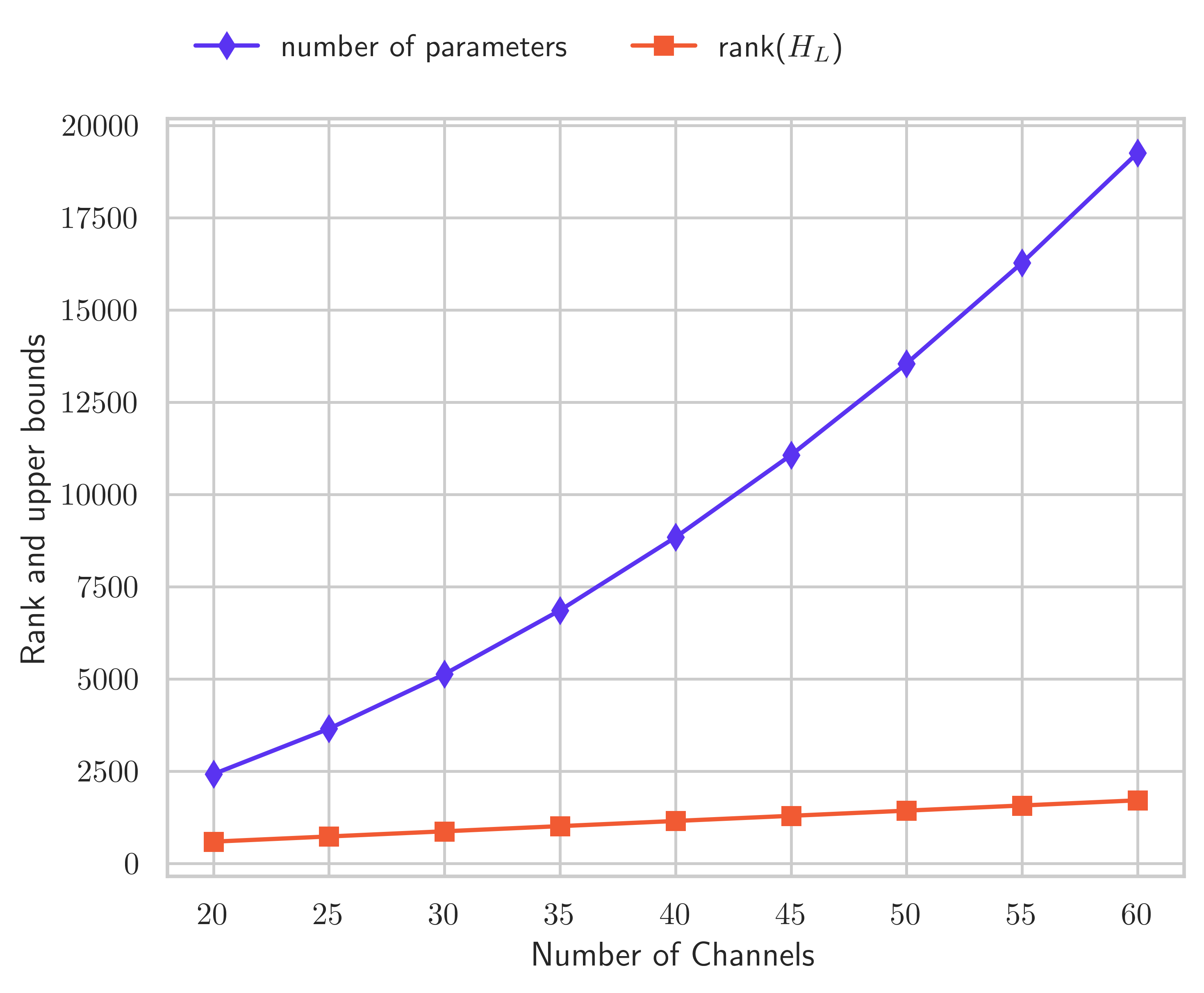
Figure 1: A comparison of the number of parameters with the empirically observed loss Hessian rank for increasing number of channels $m$ for a $2$-hidden layer CNN on CIFAR10. Can we estimate the precise scaling behaviour of the Hessian rank?

2 Related Work

The Nature of CNNs. To start with, there’s the intuitive perspective of enabling a hierarchy of features (LeCun et al., 1995). A more mathematical take is that of (Bruna & Mallat, 2013) where filters are constructed as wavelets and which as a whole provide Lipschitz continuity to deformations. The approximation theory view (Poggio et al., 2015; Mao et al., 2021) reinforces the intuitive benefits of hierarchy and compositionality with explicit constructions. On the optimization side, the implicit bias perspective (Gunasekar et al., 2018) stresses on how gradient descent on CNNs leads to a particular solution. Other notable takes are from the viewpoint of Gaussian processes (Garriga-Alonso et al., 2018), loss landscapes (Nguyen & Hein, 2018; Gu et al., 2020), arithmetic circuits (Cohen & Shashua, 2016) — to list a few. In contrast, we focus on how, from the initialization itself, the CNN architecture induces structural properties of the loss Hessian and by extension, of the loss landscape.

Hessian maps and Deep Learning. The Hessian characterizes parameter interactions via second derivative of the loss. Consequently, it has been a central object of study and has been extensively utilized for applications and theory alike, both in the past as well as the present. For instance, generalization (MacKay, 1992a; Keskar et al., 2016; Yang et al., 2019; Singh et al., 2022), optimization (Zhu et al., 1997; Setiono & Hui, 1995; Martens & Grosse, 2015; Cohen et al., 2021), network compression (LeCun et al., 1990; Hassibi & Stork, 1992; Singh & Alistarh, 2020), continual learning (Kirkpatrick et al., 2017), hyperparameter search (LeCun et al., 1992; Schaul et al., 2013), and more.

In recent times, it has been revitalized in significant part due to the ‘flatness hypothesis’ (Keskar et al., 2016; Hochreiter & Schmidhuber, 1997) and in turn, flatness has become a popular method to probe the extent of generalization as it seems to consistently rank ahead of traditional norm-based complexity measures (Jiang et al., 2019) in multiple scenarios. Given the increasing size of the networks, and the inherent limitation of the Hessian being quadratic in cost, measuring flatness has almost become synonymous with measuring the top eigenvalue of the Hessian (Cohen et al., 2021) or even just the zeroth-order measurement of the loss stability in the parameter space. To a lesser extent, some works still utilize efficient approximations to the Hessian trace (Yao et al., 2020) or log determinant (Jia & Su, 2020). But largely the reliance on the Hessian for neural networks has become a black-box affair.

Understanding of the Neural Network Hessian maps. Lately, significant advances have been made in this direction — a few of the most prominent being: the characterization of its spectra as bulk and outliers (Sagun et al., 2016; Pennington & Bahri, 2017; Ghorbani et al., 2019), the empirically observed significant rank degeneracy (Sagun et al., 2017), and the class/cross-class structure (Papyan, 2020). Despite these advancements, its structure for neural networks primarily gets seen only up to the surface level of the chain rule  for a composition of functions, with a few exceptions such as (Wu et al., 2020; Singh et al., 2021).

We take our main inspiration from the latter of these works, namely (Singh et al., 2021), where the authors precisely characterize the structure for deep fully-connected networks (FCNs) resulting in concise bounds and formulae on the Hessian rank of arbitrary sized networks. Our aim, thus, is to thoroughly exhibit the structure of the Hessian for deep convolutional networks and explore the distinctive facets that arise in CNNs — as compared to FCNs.

Our contributions: (1) We develop a framework to analyze CNNs that rests on a Toeplitz representation of convolution and applies for general deep, multi-channel, arbitrary-sized CNNs, while being amenable to matrix analysis. We then utilize this framework to unravel the Hessian structure for CNNs and provide upper bounds on the Hessian rank. Our bounds are exact for the case of 1-hidden layer CNNs, and in the general case, are of the order of square root of the trivial bounds.

(2) Next, we verify our bounds empirically in a host of settings, where we find that our upper bounds remain rather close to the true empirically observed Hessian rank. Moreover, they even hold faithfully outside the confines of the theoretical setting (choice of loss and activation functions) used to derive them.

(3) Further, we make a detailed comparison of the key ingredients in CNNs, i.e., local connectivity and weight sharing, in a simplified setting through the perspective of our Hessian results. We also discuss some elements of our proof technique in the hope that it helps provide a better grasp of the results.

We would also like to make a quick remark about the difference with regards to (Singh et al., 2021). While we borrow heavily from their approach, the framework we develop here provides us with the flexibility to handle convolutions, pooling operations, and even fully-connected layers. In particular, our analysis captures their results as a special case when the filter size is equal to the spatial dimension. We also introduce a novel proof technique relative to (Singh et al., 2021), without which one cannot attain exact bounds on the Hessian rank for the one-hidden layer case.

Overall, we hope that by building on the prior work, we can further push this research direction of understanding the nature of various network architectures through an in-depth, white-box, analysis of the Hessian structure.

3 Setup and Background

Notation.

We denote vectors in lowercase bold ($\mathbf{x}$), matrices in uppercase bold (${\bf X}$), and tensors in calligraphic letters ($\mathcal{X}$). We will denote the $i$-th row and $j$-th columns of some matrix ${\bf A}$ by ${{\bf A}}_{i\,\bullet}$ and ${{\bf A}}_{\bullet\,j}$ respectively. We will often use the notation ${\bf A}^{(i:j)}$, for $i>j$ to indicate a sequence of matrices from $i$ down to $j$, i.e., ${\bf A}^{(i:j)}={\bf A}^{(i)}{\bf A}^{(i-1)}\cdots{\bf A}^{(j+1)}{\bf A}^{(j)}$. For $i<j$, the same notation would mean the sequence of matrices from $i$ up to $j$, but tranposed. To express the structure of the gradients and the Hessian, we will employ matrix derivatives (Magnus & Neudecker, 2019), wherein we vectorize row-wise ($\operatorname{vec}_{r}$) the involved matrices and organize the derivative in Jacobian (numerator layout). Concretely, for matrices ${\bf X}\in{\mathbb{R}^{m\times n}}$ and ${\bf Y}\in{\mathbb{R}^{p\times q}}$, we have

$$\dfrac{\partial{\bf Y}}{\partial{\bf X}}:=\dfrac{\partial\operatorname{vec}_{r}{\bf Y}}{\partial\,(\operatorname{vec}_{r}{\bf X})^{\top}}\in{\mathbb{R}^{pq\times mn}}\,.$$

Setting.

Suppose we are given an i.i.d. dataset $S=\{(\mathbf{x}_{1},\mathbf{y}_{1}),\dots,(\mathbf{x}_{n},\mathbf{y}_{n})\}$, of size $|S|=n$, drawn from an unknown distribution $p_{{\mathbb{X}},{\mathbb{Y}}}$, consisting of inputs $\mathbf{x}\in{\mathbb{X}}\subseteq\mathbb{R}^{d}$ and targets $\mathbf{y}\in{\mathbb{Y}}\subseteq\mathbb{R}^{K}$. Based on this dataset $S$, consider we use a neural network to learn the mapping from the inputs to the targets, $\mathrm{F}_{{\boldsymbol{\theta}}}:{\mathbb{X}}\mapsto{\mathbb{Y}}$, parameterized by ${\boldsymbol{\theta}}\in{\boldsymbol{\Theta}}\subseteq\mathbb{R}^{p}$. To this end, we follow the framework of Empirical Risk Minimization (Vapnik, 1991), and optimize a suitable loss function ${\mathrm{L}}:\Theta\mapsto\mathbb{R}$. In other words, we solve the following optimization problem,

$${{\boldsymbol{\theta}}^{\star}}=\operatorname*{argmin}_{{\boldsymbol{\theta}}\in{\boldsymbol{\Theta}}}\;{\mathrm{L}}({\boldsymbol{\theta}})=\dfrac{1}{n}\sum\limits_{i=1}^{n}\ell\left({\boldsymbol{\theta}};(\mathbf{x}_{i},\mathbf{y}_{i})\right)\,,$$

say with a first-order method like (stochastic) gradient descent and the choices for $\ell$ could be mean-squared error (MSE), cross-entropy (CE), etc.

Hessian.

We analyze the properties of the Hessian of the loss function, ${\mathbf{H}_{{\mathrm{L}}}}=\dfrac{\partial^{2}{\mathrm{L}}({\boldsymbol{\theta}})}{\partial{\boldsymbol{\theta}}\,\partial{\boldsymbol{\theta}}{}^{\top}}$, with respect to the parameters ${\boldsymbol{\theta}}$. It is quite well known (Schraudolph, 2002a; Sagun et al., 2017) that, via the chain rule, the Hessian can be decomposed as a sum of the following two matrices:

$${\mathbf{H}_{{\mathrm{L}}}}=\mathbf{H}_{\mathrm{O}}+{\mathbf{H}_{\mathrm{F}}} =\frac{1}{n}\sum_{i=1}^{n}\nabla_{{\boldsymbol{\theta}}}\mathrm{F}_{{\boldsymbol{\theta}}}(\mathbf{x}_{i})\big{[}\nabla^{2}_{\mathrm{F}_{{\boldsymbol{\theta}}}}\,\ell_{i}\big{]}\,\nabla_{\boldsymbol{\theta}}\mathrm{F}_{{\boldsymbol{\theta}}}(\mathbf{x}_{i})^{\top}$$

$$+\frac{1}{n}\sum_{i=1}^{n}\,\sum_{c=1}^{K}[\nabla_{\mathrm{F}_{{\boldsymbol{\theta}}}}\ell_{i}]_{c}\,\nabla^{2}_{\boldsymbol{\theta}}\,\mathrm{F}_{{\boldsymbol{\theta}}}^{c}(\mathbf{x}_{i})$$ (1)

where, $\nabla_{\boldsymbol{\theta}}\mathrm{F}_{{\boldsymbol{\theta}}}(\mathbf{x}_{i})\in\mathbb{R}^{p\times K}$ is the Jacobian of the function and $\nabla^{2}_{\mathrm{F}_{{\boldsymbol{\theta}}}}\,\ell_{i}\in\mathbb{R}^{K\times K}$ is the Hessian of the loss with respect to the network function, at the $i$-th sample. To facilitate comparison, we refer to these two matrices as the outer-product Hessian and the functional Hessian following (Singh et al., 2021).

3.1 Background

Precise bounds on the Hessian rank.

Despite the much interest in Hessian over the decades, the upper bounds remained quite trivial (like a factor of the number of samples) and the empirically observed degeneracy (Sagun et al., 2016), because of the need to measure rather small eigenvalues and judge a suitable threshold, remained intractable to establish. Exact upper bounds and formulae have only been made available very recently for fully-connected networks due to (Singh et al., 2021), as a result of subtle choice to have linear activations, together with a novel analysis technique adapted from matrix analysis (Matsaglia & Styan, 1974; Chuai & Tian, 2004). While they find that the presence of non-linearities like ReLU impedes a theoretical analysis, (Singh et al., 2021) thoroughly demonstrate that their bounds hold empirically for ReLU-based FCNs as well. Their empirical analysis is equally rigorous, for they compute exact Hessians (without any approximation) in Float64 precision.

Overall, the surprising finding of (Singh et al., 2021) is that the Hessian rank for FCNs scales linearly in the total number of neurons $m$, i.e., $\mathcal{O}(m)$; while the number of parameters scale quadratically, $\mathcal{O}(m^{2})$. While this concrete bound of $\mathcal{O}(m)$ is shown at initialization, their analysis applies to any point during training — but with resulting bound in terms of the rank of the individual weight matrices. Further, they highlight that during training, the rank can only decrease (a simple consequence of the functional Hessian ${\mathbf{H}_{\mathrm{F}}}$ being driven to zero since it is scaled by the gradient of the loss $\nabla_{\mathrm{F}_{{\boldsymbol{\theta}}}}\ell$). In this sense, their upper bounds hold pointwise throughout the loss landscape.

Why Hessian Rank?

The finding about the growth of Hessian rank carries thought-provoking implications on the number of effective parameters within a particular architecture. Let us illustrate this by considering the Occam’s factor (MacKay, 1992b; Gull, 1989) which, said roughly, describes the extent to which the prior hypothesis space shrinks on observing the data. More formally, this is the ratio of posterior to prior volumes in the parameter space. This is then used to derive the following measure for the effective degrees of freedom, assuming a quadratic approximation to the posterior: $\sum\limits_{i=1}^{p}\dfrac{\lambda_{i}}{\lambda_{i}+\epsilon}\,,$ where, $\lambda_{i}$ denotes the $i$-th eigenvalue of the Hessian, $p$ is the total number of parameters, and $\epsilon$ is the weight set upon the prior. In other words, the above measure compares the extent ($\lambda_{i}$) to which a particular direction (along the $i$-th eigenvector) in the parameter space is determined by the data relative to that determined by the prior $\epsilon$. For small $\epsilon$, which amounts to little or no explicit regularization towards the prior (as is often the case with deep networks in practice), this measure of the degrees of freedom approaches the Hessian rank. In a recent work (Maddox et al., 2020) empirically noted that this measure also explains double descent (Belkin et al., 2019) in neural networks. Thus, it makes it all the more pertinent to explore how rank of the Hessian scales with various architectural parameters in a CNN.

4 Toeplitz Framework for CNN Hessians

Preliminaries. In this section, we will lay out the formalism that will lie at the core of our analysis. For brevity, we will develop this in the case of 1D CNNs which are commonly employed for biomedical applications or audio data (Kiranyaz et al., 2021). One can otherwise think of applying our framework to flattened filters and input patches, and such an assumption is also prevalent in the theory literature (Kohn et al., 2021). Besides, throughout our framework we will assume there are no bias parameters, although one can simply consider homogeneous coordinates in the input.

Warmup.

Let’s say we want to represent the convolution ${\bf W}*\mathbf{x}$ of an input $\mathbf{x}\in{\mathbb{R}^{d}}$ with $m$ filters of size $k\leq d$ that have been organized in the matrix ${\bf W}\in{\mathbb{R}^{m\times k}}$. For now, consider that we have stride $1$ and zero padding. We will later touch upon these aspects and see the results for strides $>1$ in Section 7. Further, for some vector $\mathbf{z}\in{\mathbb{R}^{d}}$, we will use the notation $\mathbf{z}_{j:j+k-1}\in{\mathbb{R}^{k}}$ to denote the (shorter) vector formed by considering the indices $j$ to $j+k-1$ (both inclusive) of the original vector. The output of the above convolution can be expressed as the following matrix of shape $m\times(d-k+1)$,

$$\small{\bf W}\ast\mathbf{x}=\begin{pmatrix}\langle{{\bf W}}_{1\,\bullet},\,\mathbf{x}_{1:k}\rangle&\cdots&\langle{{\bf W}}_{1\,\bullet},\,\mathbf{x}_{d-k+1:d}\rangle\\[5.69054pt] \vdots&&\vdots\\[5.69054pt] \langle{{\bf W}}_{m\,\bullet},\,\mathbf{x}_{1:k}\rangle&\cdots&\langle{{\bf W}}_{m\,\bullet},\,\mathbf{x}_{d-k+1:d}\rangle\end{pmatrix}\,.$$ (2)

Now, define Toeplitz matrices for each filter, $\{{{\bf T}}^{{{\bf W}}_{i\,\bullet}}\}_{i=1}^{m}$, with ${{\bf T}}^{{{\bf W}}_{i\,\bullet}}:=\operatorname{toep}({{\bf W}}_{i\,\bullet},d)\in{\mathbb{R}^{(d-k+1)\times d}}$ such that,

$$\small{{\bf T}}^{{{\bf W}}_{i\,\bullet}}=\begin{pmatrix}w_{i1}&\cdots&w_{ik}&0&\cdots&0\\[5.69054pt] 0&w_{i1}&\cdots&w_{ik}&0&\vdots\\[5.69054pt] \vdots&0&\ddots&\ddots&\ddots&0\\[5.69054pt] 0&\cdots&0&w_{i1}&\cdots&w_{ik}\\[5.69054pt] \end{pmatrix}\,.$$

Note, the above representation of the Toeplitz matrix also depends on the base dimension (here, $d$) where the given vector must be ‘toeplitzed’, i.e., circulated in the above fashion. But we will omit specifying this unless necessary. Let us also denote the matrix formed by stacking the ${{\bf T}}^{{{\bf W}}_{i\,\bullet}}$ matrices in a row-wise fashion as

$$\small{{\bf T}}^{{\bf W}}:=\begin{pmatrix}{{\bf T}}^{{{\bf W}}_{1\,\bullet}}\\[2.84526pt] \vdots\\[2.84526pt] {{\bf T}}^{{{\bf W}}_{m\,\bullet}}\\[2.84526pt] \end{pmatrix}\,\in{\mathbb{R}^{m(d-k+1)\times d}}\,.$$

We can now see that the above matrix, ${{\bf T}}^{{\bf W}}$, when multiplied by the input $\mathbf{x}$ gives us the output of the convolution operation in Eqn. (2) when vectorized row-wise , i.e.,

$$\operatorname{vec}_{r}({\bf W}*\mathbf{x})={{\bf T}}^{{\bf W}}\mathbf{x}\,.$$

4.1 Toeplitz representation of deep CNNs

Now, let us assume we have $L$ hidden layers, each of which is a convolutional kernel. Hence, the parameters of the $l$-th layer are denoted by the tensor ${\mathcal{W}}^{(l)}\in{\mathbb{R}^{m_{l}\times m_{l-1}\times k_{l}}}$, where $m_{l}$ represent the number of output channels, $m_{l-1}$ the number of input channels, and $k_{l}$ the kernel size at this layer. As we assume a one-dimensional input, without loss of generality, we can set the number of input channels $m_{0}=1$. In other words, they are already assumed to be flattened when passing the input of dimension $d_{0}:=d$ into the network. The spatial dimension after being convolved with the $l$-th layer is denoted by $d_{l}=d_{l-1}-k_{l}+1$ (which is basically the number of hops we can make with the given kernel over its respective input), since we have stride $1$ and zero padding. Assume, say the ReLU nonlinearity $\sigma(x):=\max(x,0)$. The network function can then be formally represented as (although it will be actually defined through Eqn. (3) later):

$$\mathrm{F}_{{\boldsymbol{\theta}}}(\mathbf{x})={\mathcal{W}}^{(L+1)}\ast\sigma({\mathcal{W}}^{(L)}\ast\sigma(\,\cdots\ast\sigma({\mathcal{W}}^{(1)}\ast\mathbf{x})))\,.$$

As before, we would like to express the above function in terms of a sequence of appropriate Toeplitz matrix products. Unlike the warmup scenario, the convolutional kernels in this general case will be tensors. The key idea is to do a column-wise stacking of individual Toeplitz matrices across the input channels while maintaining the row-wise stacking, as before, across the output channels.

First, we need to introduce a notation about indexing the fibres of a tensor ${\mathcal{W}}^{(l)}\in{\mathbb{R}^{m_{l}\times m_{l-1}\times k_{l}}}$. Say we need the fibre going in to the plane, across the third mode. Then, the $(i,j)$-th fibre is denoted by ${\mathcal{W}^{(l)}_{(i,j)\,\bullet}}\in{\mathbb{R}^{k_{l}}}$, whose associated Toeplitz matrix will be ${{\bf T}}^{{\mathcal{W}^{(l)}_{(i,j)\,\bullet}}}:=\operatorname{toep}({\mathcal{W}^{(l)}_{(i,j)\,\bullet}},d_{l-1})\in{\mathbb{R}^{d_{l}\times d_{l-1}}}$. Finally, the Toeplitz matrix associated with the entire $l$-th convolutional layer ${\mathcal{W}}^{(l)}$, for which we use the shorthand ${{\bf T}}^{(l)}\in{\mathbb{R}^{m_{l}d_{l}\times m_{l-1}d_{l-1}}}$, can be expressed as:

$${{{\bf T}}^{(l)}:=\begin{pmatrix}{{\bf T}}^{{\mathcal{W}^{(l)}_{(1,1)\,\bullet}}}&\cdots&{{\bf T}}^{{\mathcal{W}^{(l)}_{(1,m_{l-1})\,\bullet}}}\\[2.84526pt] \vdots&&\vdots\\[2.84526pt] {{\bf T}}^{{\mathcal{W}^{(l)}_{(m_{l},1)\,\bullet}}}&\cdots&{{\bf T}}^{{\mathcal{W}^{(l)}_{(m_{l},m_{l-1})\,\bullet}}}\\[2.84526pt] \end{pmatrix}\,.}$$

In other words, the Toeplitzed representation ${{\bf T}}^{(l)}$ consists of $m_{l}\cdot m_{l-1}$ many Toeplitz blocks formed by the vector ${\mathcal{W}^{(l)}_{(i,j)\,\bullet}}\in{\mathbb{R}^{k_{l}}}$ of size $d_{l}\times d_{l-1}$. The output (spatial) dimension $d_{L+1}$ is typically 1 (corresponding to $k_{L+1}=d_{L}$), and the number of output channels for the last layer $m_{l+1}=K$ where $K$ is the number of targets. Now, the network function can be written in the general case as:

$$\mathrm{F}_{{\boldsymbol{\theta}}}(\mathbf{x})={{\bf T}}^{(L+1)}\Lambda^{(L)}{{\bf T}}^{(L)}\cdots\Lambda^{(1)}{{\bf T}}^{(1)}\,\mathbf{x}\,,$$ (3)

where, $\Lambda^{(i)}$ is an input-dependent diagonal matrix that contains a $1$ or $0$, based on whether the neuron was activated or not. As the rank analysis of (Singh et al., 2021) requires linear activations, we will follow the same course. However, we can expect that this should still let us contrast the distinctive facets of CNN relative to a FCN. Anyways, later we will elaborate on the case of nonlinearities. Besides, we will refer to the above network function, more concisely as ${{\bf T}}^{(L+1:1)}\mathbf{x}$.

Remark. As evident, the fact that a convolution of a set of vectors can be expressed as a matrix-vector product with a suitable Toeplitz matrix is rather straightforward. Also, a Toeplitz representation for CNN is not new — works from approximation theory incorporate a similar formalism (Zhao et al., 2017; Fang et al., 2020). However, unlike past work (Sedghi et al., 2018; Kohn et al., 2021), we develop our framework in a way that doesn’t overlook how convolutions are prominently used, i.e., without circular convolution, with multiple channels, and possibly unequal-sized layers.

4.2 Matrix derivatives of Toeplitz representations

For the gradient and Hessian calculations, we make use of matrix derivatives and the corresponding chain rule. Thus we frequently compute the gradient of the Toeplitz representation ${{\bf T}}^{(l)}$ with respect to the suitably matricized convolutional tensor, $\operatorname{mat}{\mathcal{W}}^{(l)}$. In order to be consistent with the form of ${{\bf T}}^{(l)}$, we define our matricization of ${\mathcal{W}}^{(l)}$ as:

$$\small\operatorname{mat}{{\mathcal{W}}^{(l)}}:=\begin{pmatrix}{{\mathcal{W}^{(l)}_{(1,1)\,\bullet}}}&\cdots&{{\mathcal{W}^{(l)}_{(m_{l},1)\,\bullet}}}\\ \vdots&&\vdots\\ {{\mathcal{W}^{(l)}_{(1,m_{l-1})\,\bullet}}}&\cdots&{{\mathcal{W}^{(l)}_{(m_{l},m_{l-1})\,\bullet}}}\end{pmatrix}^{\top}\,.$$ (4)

where the matricization $\operatorname{mat}{{\mathcal{W}}^{(l)}}\in{\mathbb{R}^{m_{l}\times m_{l-1}k_{l}}}$ and we will use the notation $\mathbf{W}^{(l)}:=\operatorname{mat}{{\mathcal{W}}^{(l)}}$ as a shorthand. Essentially, we have arranged each of the mode-$3$ fibres as rows in the output channels times input channels format.

The following lemma equips us with the way to carry this out (the proof can be found in Section A.1 of the Appendix).

Lemma 1.

The matrix derivative of ${{\bf T}}^{(l)}$ with respect to $\mathbf{W}^{(l)}$, is given as follows:

$$\widetilde{{\bf Q}}^{(l)}:=\dfrac{\partial{{\bf T}}^{(l)}}{\partial\mathbf{W}^{(l)}}:=\dfrac{\partial\operatorname{vec}_{r}{{\bf T}}^{(l)}}{\partial\left(\operatorname{vec}_{r}\mathbf{W}^{(l)}\right)^{\top}}={\bf I}_{m_{l}}\,\mathbin{\mathop{\otimes}}\,{{\bf Q}}^{(l)}\,.$$

The particular structure of ${{\bf Q}}^{(l)}$ is a bit complex, involving various permutation matrices. So, for simplicity, we abstract it out here in the main text.

4.3 CNN Hessian Structure

Like (Singh et al., 2021), for our theoretical analysis, we will consider the case of MSE loss. But the results still hold empirically, say, for CE loss. Let’s now have a glance at the $kl$-th block, $k\leq l$ for both the outer-product and the functional Hessian (the derivations are in Section LABEL:sec:struct). This corresponds to looking at the submatrix of the Hessian corresponding to the $k$-th and $l$-th convolutional parameter tensors. Let’s start with the outer-product Hessian $\mathbf{H}_{\mathrm{O}}$.

Proposition 2.

The $kl$-th block of $\mathbf{H}_{\mathrm{O}}$ is,

$${\mathbf{H}^{(kl)}_{\mathrm{O}}} ={{\widetilde{{\bf Q}}}^{(k)}{}^{\top}}\bigg{(}{{\bf T}}^{(k+1:L+1)}{{\bf T}}^{(L+1:l+1)}\,\,\mathbin{\mathop{\otimes}}$$

$$\hskip 50.00008pt{{\bf T}}^{(k-1:1)}{\bm{\Sigma}_{\mathbf{x}\mathbf{x}}}{{\bf T}}^{(1:l-1)}\bigg{)}{{\widetilde{{\bf Q}}}^{(l)}}\,.$$ (5)

A word about $\mathbf{H}_{\mathrm{O}}$. We should also emphasize that the outer-product Hessian shares exactly the same non-zero spectrum as the Neural Tangent Kernel (Jacot et al., 2018), or roughly up to scaling, in the case of Fisher Information (Amari, 1998), empirical Fisher (Kunstner et al., 2019)).

Moving on to the functional Hessian ${\mathbf{H}_{\mathrm{F}}}$, denote ${\mathbf{\Omega}}=\mathbf{E}\,[\boldsymbol{\delta}_{\mathbf{x},\mathbf{y}}\,\mathbf{x}^{\top}]\in{\mathbb{R}^{K\times d_{0}}}$ as the (uncentered) covariance of the residual $\left(\mathbf{y}_{i}-\mathrm{F}_{{\boldsymbol{\theta}}}(\mathbf{x}_{i})\right)$ with the input. Then we have,

Proposition 3.

The $kl$-th block of ${\mathbf{H}_{\mathrm{F}}}$ is:

$${\mathbf{H}_{\mathrm{F}}^{(kl)}} =\left({\bf I}_{m_{k}}\mathbin{\mathop{\otimes}}{{\bf Q}}^{(k)}{}^{\top}\right)\bigg{(}{{\bf T}}^{(k+1:l-1)}\,\,\mathbin{\mathop{\otimes}}$$

$$\hskip 30.00005pt{{\bf T}}^{(k-1:1)}{\mathbf{\Omega}}^{\top}{{\bf T}}^{(L+1:l+1)}\bigg{)}\left({{\bf Q}}^{(l)}\mathbin{\mathop{\otimes}}{\bf I}_{m_{l}}\right)\,,$$ (6)

A word about ${\mathbf{H}_{\mathrm{F}}}$. As the outer-product Hessian is positive semi-definite, the functional Hessian is the source of all the negative eigenvalues of the Hessian and is important for optimization as there may be numerous saddles in the landscape (Dauphin et al., 2014). It also has a very peculiar block-hollow structure (i.e., zero diagonal blocks), which leads to the number of negative eigenvalues being approximately half of its rank (c.f., (Singh et al., 2021)).

5 Key results on the CNN Hessian Rank

Finally, we can now present our key results. A quick note about assumptions: for simplicity, assume that the (uncentered) input-covariance ${\bm{\Sigma}_{\mathbf{x}\mathbf{x}}}=\operatorname{cov}(\mathbf{x})$ has full rank $\operatorname{rank}\left({\bm{\Sigma}_{\mathbf{x}\mathbf{x}}}\right):=r=d$. We will analyze the ranks of the outer product and functional Hessian, later combining them to yield a bound on the rank of the loss Hessian. This is without loss of generality for one can always pre-process the input to ensure that this is the case, and results of (Singh et al., 2021) hold for $r\neq d$ with appropriate modifications.

Outer-Product Hessian $\mathbf{H}_{\mathrm{O}}$. From the structure of the $kl$-th block in Eqn. (2), it’s easy to see to arrive at the following proposition:

Proposition 4.

For a deep linear convolutional network, $\,\mathbf{H}_{\mathrm{O}}={\bf Q}_{o}^{\top}{\bf A}_{o}{\bf B}_{o}{{\bf A}_{o}^{\top}}{\bf Q}_{o}\,$, where $\,{\bf B}_{o}={\bf I}_{K}\mathbin{\mathop{\otimes}}{\bm{\Sigma}_{\mathbf{x}\mathbf{x}}}\,\in\mathbb{R}^{Kd\times Kd}$, $\,\,\,{\bf A}_{o}^{\top}=\begin{pmatrix}{{\bf T}}^{(L+1:2)}\mathbin{\mathop{\otimes}}{\bf I}_{d}\\[2.84526pt] \vdots\\[2.84526pt] {{\bf T}}^{(L+1:l+1)}\mathbin{\mathop{\otimes}}{{\bf T}}^{(1:l-1)}\\[2.84526pt] \cdots\\[2.84526pt] {\bf I}_{K}\mathbin{\mathop{\otimes}}{{\bf T}}^{(1:L)}\end{pmatrix}\,\,\in\mathbb{R}^{Kd\times\widehat{p}}\,,$ and ${\bf Q}_{o}=\operatorname{diag}\left(\widetilde{{\bf Q}}^{(1)},\cdots,\widetilde{{\bf Q}}^{(L+1)}\right)\in{\mathbb{R}^{\widehat{p}\times p}}$ where $\operatorname{diag}(\cdot)$ denotes a block-diagonal matrix.

Besides, $p=\sum_{i=1}^{L+1}m_{l}m_{l-1}{k_{l}}$ and $\widehat{p}=\sum_{i=1}^{L+1}m_{l}m_{l-1}d_{l}d_{l-1}$. The former denotes the number of parameters in the CNN while the latter is the number of parameters in the ‘Toeplitzed’ fully-connected network.

Our first key result, the proof of which is located in Section LABEL:sec:ho-cnn-proof of the Appendix, can then be described as follows :

Theorem 5.

The rank of the outer-product Hessian is upper bounded as $\displaystyle\operatorname{rk}(\mathbf{H}_{\mathrm{O}})$ $\displaystyle\leq\min\big{(}p,d_{0}\operatorname{rk}({{\bf T}}^{(2:L+1)})+K\operatorname{rk}({{\bf T}}^{(L:1)})\,-$ $\displaystyle\hskip 50.00008pt\operatorname{rk}({{\bf T}}^{(2:L+1)})\operatorname{rk}({{\bf T}}^{(L:1)})\big{)}$ $\displaystyle=\min\left(p,q\,(d_{0}+K-q)\right)\,.$ Here, $q:=\min(d_{0},m_{1}d_{1},\cdots,m_{L}d_{L},K)$.

Assuming no bottleneck layer, we will have that $q=\min(d,K)$, and resulting in $\operatorname{rk}(\mathbf{H}_{\mathrm{O}})\leq Kd_{0}$.

Functional Hessian ${\mathbf{H}_{\mathrm{F}}}$.

Our approach here will be similar to that in the Theorem above. We will try to factor out all the ${{\bf Q}}^{(l)}$ matrices and then analyze the rank of the resulting decomposition. But, this requires more care as the form of the $kl$-th block is different depending on $k\leq l$ or not.

Theorem 6.

For a deep linear convolutional network, the rank of $l$-th column-block, ${\widehat{\mathbf{H}}_{\mathrm{F}}^{\bullet l}}$, of the matrix ${\widehat{\mathbf{H}}_{\mathrm{F}}}$, can be upper bounded as $$\operatorname{rk}({\widehat{\mathbf{H}}_{\mathrm{F}}^{\bullet l}})\leq\min(\widehat{q}\,m_{l-1}d_{l-1}+\widehat{q}\,m_{l}d_{l}-\widehat{q}^{\,2}\,,m_{l}m_{l-1}k_{l})\,,$$ for $l\in[2,\cdots,L]\,.$ When $l=1$, we have $$\operatorname{rk}({\widehat{\mathbf{H}}_{\mathrm{F}}^{\bullet 1}})\leq\min(\widehat{q}\,m_{1}d_{1}+\widehat{q}\,s-\widehat{q}^{\,2}\,,m_{1}m_{0}k_{1})\,.$$ And, when $l=L+1$, we have $$\operatorname{rk}({\widehat{\mathbf{H}}_{\mathrm{F}}^{\bullet L+1}})\leq\min(\widehat{q}\,m_{L}d_{L}+\widehat{q}\,s-\widehat{q}^{\,2}\,,m_{L+1}m_{L}k_{L+1})\,.$$ Here, $\widehat{q}:=\min(d_{0},m_{1}d_{1},\cdots,m_{L}d_{L},K,s)=\min(q,s)$ and $s:=\operatorname{rk}({\mathbf{\Omega}})=\operatorname{rk}(\mathbf{E}\,[\boldsymbol{\delta}_{\mathbf{x},\mathbf{y}}\,\mathbf{x}^{\top}])$.

The proof is located in Section LABEL:sec:hf-cnn-proof of the Appendix. The upper bound on the rank of ${\mathbf{H}_{\mathrm{F}}}$ follows by summing the above result over all the columns, $\operatorname{rk}({\mathbf{H}_{\mathrm{F}}})\leq\sum\limits_{l=1}^{L+1}\operatorname{rk}({\widehat{\mathbf{H}}_{\mathrm{F}}^{\bullet l}})$ by the sub-additivity of rank. A remarkable empirical observation, like in the case of FCNs, is that the block-columns are mutually orthogonal — hence, we don’t loose anything by simply summing the ranks of the block columns.

Loss Hessian ${\mathbf{H}_{{\mathrm{L}}}}$. One can then bound the rank of the loss Hessian simply as, $\operatorname{rk}({\mathbf{H}_{{\mathrm{L}}}})\leq\operatorname{rk}(\mathbf{H}_{\mathrm{O}})+\operatorname{rk}({\mathbf{H}_{\mathrm{F}}})$. Also, we can infer that, in the likely case where $q=\min(K,d_{0})$, rank of the loss Hessian grows linearly with number of channels, i.e., $\mathcal{O}(m\cdot L\cdot d_{0})$, while the number of parameters grow quadratically in the number of channels, i.e., $\mathcal{O}(m^{2}\cdot L\cdot d_{0})$. Thereby, we confirm that like FCNs, a similar linear trend also holds for CNNs (and hence the Figure 1). Besides, for very large networks, $m$ will be the dominating factor and we can infer that rank will show a square root behaviour relative to the number of parameters. Hence, we generalize the key finding of (Singh et al., 2021) in the fully-connected case to the case of convolutional neural networks.

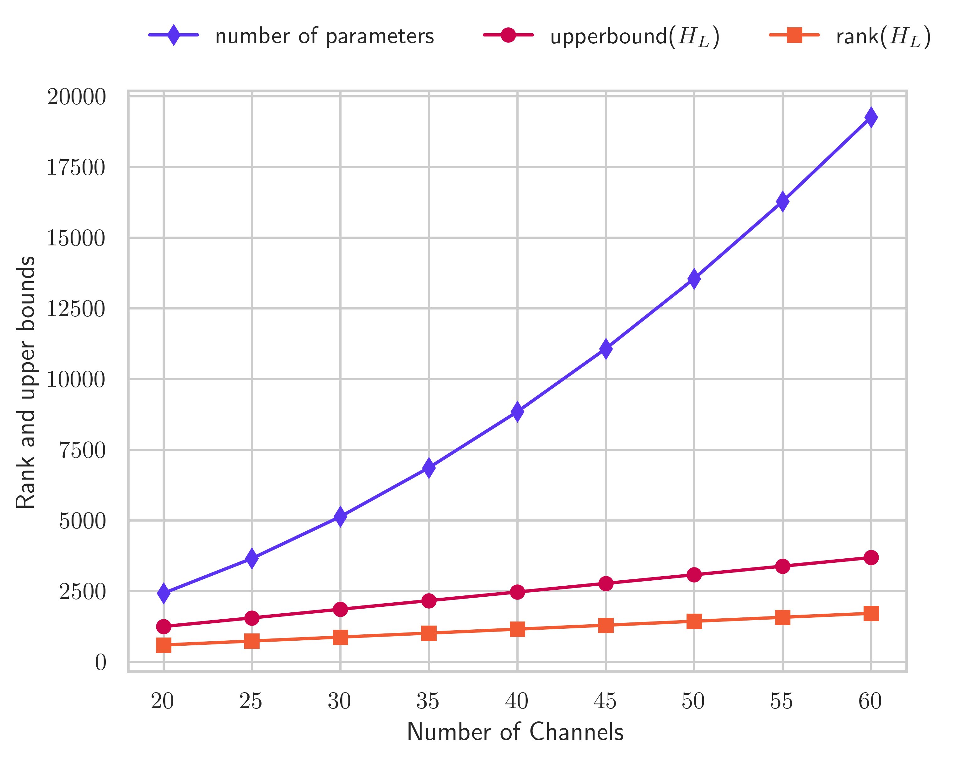
(a) Linear CNN: Rank vs # Channels

(b) Linear CNN: Rank vs Filter size

(c) ReLU CNN: Rank vs Filter size

Figure 2: Trend of the upper bound on the (loss) Hessian rank, compared to the true rank, and the number of parameters. In other subfigures, we see the rank of the functional Hessian and outer-product Hessian.

5.1 Exact results for one-hidden layer case

While the above bounds are much tighter than any existing bounds, we now try to understand how tight our bounds are by looking at the case of a 1-hidden layer:

Theorem 7.

The rank of the outer product Hessian can be bounded as: $\operatorname{rank}\left(\mathbf{H}_{\mathrm{O}}\right)\leq\min\big{(}Kd_{0},q(k_{1}+K(d_{0}-k_{1}+1)-q)\big{)}\,$, where $q=\min(k_{1},K(d_{0}-k_{1}+1),m_{1})$.

Theorem 8.

The rank of the functional Hessian is bounded as: $\operatorname{rank}\left({\mathbf{H}_{\mathrm{F}}}\right)\leq 2\min\big{(}k_{1},K(d_{0}-k_{1}+1)\big{)}\,m_{1}\,.$

The strategy behind the proofs (section LABEL:sec:cnntightproofs) is to write the CNN as a superposition of the functions that act on different input patches. Now, we must also utilize the form of Toeplitz derivatives and involved auxiliary permutation matrices. In terms of the results, interestingly, we find that now the filter size $k_{1}$ has entered inside the $\min$ terms in each of the bounds; thereby further reducing the rank. However, as shown ahead, for larger networks with many channels $m$, we find that our earlier upper bound still fares decently.

6 Empirical Verification

Verification of upper bounds.

We empirically validate our upper bounds in a variety of settings, in particular, with both linear and ReLU activations, MSE and CE loss, as well as on datasets such as CIFAR10, FashionMNIST, MNIST, and a synthetic dataset. However, given the page constraints, we only show a selection of the plots, while the rest can be found in the Appendix LABEL:sec:figures. Following (Singh et al., 2021), to rigorously illustrate the match with our bounds, we compute the exact Hessians, without approximations, and in Float64 precision. These precautions are taken to avoid any imprecision in calculating the rank, since the boundary of non-zero eigenvalues with zero can be otherwise a bit blurry.

Rank vs number of channels.

We begin by illustrating the trend of our general upper bounds in Figure 2(a) for the case of 2-hidden layer CNN on CIFAR10 and is thus the counterpart to the Figure 1 presented before. The upper bound is relatively close to the true rank and similarly shows a linear trend with the number of channels.

Rank vs Filter Size.

Next, in Figure 2(b), we demonstrate the match of our exact bound with the rank as observed empirically. We hold the number of channels as fixed and vary the filter size. First of all, here the markers and the lines indeed coincide for the functional Hessian and outer-product Hessian. On the other hand, the loss Hessian which we bound as the sum of the ranks of $\mathbf{H}_{\mathrm{O}}$ and ${\mathbf{H}_{\mathrm{F}}}$ forms a canopy over all the empirically observed values of the rank across the filter sizes. The upper bound itself is also quite close; it becomes even closer for large values of $m$, see Section LABEL:supp:fil-lin-mse).

The case of non-linearities.

Further, in a similar comparison across filter sizes, we showcase that our bounds which were derived for linear activations still remain as valid upper bounds and form a canopy as seen in Figure 2(c).

7 Locality and Weight-sharing

We would like to do a little deep dive and explore a simplified setting, in order to gather some intuition. We study the two crucial components behind CNN, namely, local connectivity (i.e, the localized patches of the input are convolved with a possibly distinct filter) and weight sharing (where the same filter is applied to each of these patches).

Setting. Concretely, let us begin by considering the case of a one-hidden layer neural network (with linear activations for simplicity). We now try to get rid of the layer indices for the sake of clarity. So the input dimension is $d$, output dimension is $K$, filter size is $k$, number of hidden layer filters is $m$. Further, we consider non-overlapping filters, like in MLPMixer (Tolstikhin et al., 2021). In other words, the stride is set equal to the filter size $k$ and so the number of patches under consideration will be $t=d/k$, and to avoid unnecessary complexity, we assume $d$ is an integer multiple of $k$.

Locally Connected Networks (LCNs).

As the filters that get applied on the patches are distinct, let us denote them by ${{\bf W}}^{(ii)}\in\mathbb{R}^{m\times k}$ and the output layer matrix as ${\bf V}:=\begin{pmatrix}{{{\bf V}}^{(1)}}&\cdots&{{{\bf V}}^{(t)}}\end{pmatrix}$, with ${{{\bf V}}^{(i)}}\in\mathbb{R}^{K\times m}$, where the superscript denotes the index of the local patch upon which they get applied. Mathematically we can represent the resulting neural network function as (where $\mathbf{x}^{(i)}\in\mathbb{R}^{k}$ denotes the $i$-th chunk of the input):

$$\small\begin{pmatrix}{{{\bf V}}^{(1)}}&\cdots&{{{\bf V}}^{(t)}}\end{pmatrix}\,\begin{pmatrix}{{\bf W}}^{(11)}&\cdots&\bm{0}\\ \vdots&\ddots&\vdots\\[2.84526pt] \bm{0}&\cdots&{{\bf W}}^{(tt)}\\ \end{pmatrix}\,\begin{pmatrix}\mathbf{x}^{(1)}\\ \vdots\\[2.84526pt] \mathbf{x}^{(t)}\end{pmatrix}$$

We indexed the local weight matrices of the first layer as ${{\bf W}}^{(ii)}$ to reflect that it is $(i,i)$-th block on the diagonal. After carrying out the block matrix multiplication, the above formulation can also be expressed as:

$$\vspace{-3mm}\mathrm{F}_{{\boldsymbol{\theta}}}^{\text{LCN}}(\mathbf{x})=\sum\limits_{i=1}^{t}{{{\bf V}}^{(i)}}\,{{\bf W}}^{(ii)}\,\mathbf{x}^{(i)}\,.$$ (7)

We can then easily bring to our minds the case of fully-connected networks which will also contain the off-diagonal blocks and would be represented as:

$$\mathrm{F}_{{\boldsymbol{\theta}}}^{\text{FCN-large}}(\mathbf{x})=\sum\limits_{i,j=1}^{t}{{{\bf V}}^{(i)}}\,{{\bf W}}^{(ij)}\,\mathbf{x}^{(j)}\,.$$

Clearly, fully-connected networks form a generalization of locally-connected networks. Another point of comparison for LCNs in Eq. (7) with FCNs is that the former may be viewed as a superposition of $s$ distinct smaller FCNs acting on disjoin patches of the input.

$$\mathrm{F}_{{\boldsymbol{\theta}}}^{\text{LCN}}(\mathbf{x})=\sum\limits_{i=1}^{t}\,\mathrm{F}_{{\boldsymbol{\theta}}}^{\text{FCN-small}}\big{(}\mathbf{x}^{(i)}\,;\,\{{{{\bf V}}^{(i)}},{{\bf W}}^{(ii)}\}\big{)}\,.$$

In this scenario of LCNs, we get the following bounds on the rank of the outer-product and functional Hessian:

Theorem 9.

For the locally connected network as described in Eqn. (7), the rank of the outer-product and the functional Hessian can be upper bounded as follows: $\operatorname{rk}(\mathbf{H}_{\mathrm{O}}^{\text{LCN}})\leq t\cdot q(k+K-q)\,,$ and $\operatorname{rk}({\mathbf{H}_{\mathrm{F}}}^{\text{LCN}})\leq t\cdot 2m\min(k,K)$, where $q=\min(k,K,m)$ and $t=d/k$.

The proof is located in Section LABEL:sec:lcn-proofs. The neat thing about the above rank expressions is that they are identical to that obtained for the smaller fully-connected network, except where we change the input dimension from $d\rightarrow k$ and scale the bounds by a factor of $t=d/k$ (the number of smaller fully-connected that are being superpositioned). In short, even though these weight matrices must ‘act’ together in the loss, their contributions to the Hessian came out individually (i.e, ${\mathbf{H}_{\mathrm{F}}}$ and $\mathbf{H}_{\mathrm{O}}$ can be factorized as block diagonals).

Incorporating Weight Sharing (WS).

Now all the weight matrices in the first layer are shared, i.e., ${{\bf W}}^{(ii)}={\bf W}$.

$$\small\begin{pmatrix}{{{\bf V}}^{(1)}}&\cdots&{{{\bf V}}^{(t)}}\end{pmatrix}\,\begin{pmatrix}{\bf W}&\cdots&\bm{0}\\ \vdots&\ddots&\vdots\\[2.84526pt] \bm{0}&\cdots&{\bf W}\\ \end{pmatrix}\,\begin{pmatrix}\mathbf{x}^{(1)}\\ \vdots\\[2.84526pt] \mathbf{x}^{(t)}\end{pmatrix}$$ (8)

Theorem 10.

For the locally connected network with weight sharing defined in Eqn. (8), the rank of the outer-product and the functional Hessian can be bounded as: $\operatorname{rk}(\mathbf{H}_{\mathrm{O}}^{\text{LCN+WS}})\leq q(k+Kt-q)\,,$ and $\operatorname{rk}({\mathbf{H}_{\mathrm{F}}}^{\text{LCN+WS}})\leq 2m\min(k,Kt)$, where $q=\min(k,Kt,m)$ and $t=d/k$.

The proof can be found in Section LABEL:sec:lcn+ws-proofs, but the intuition is that the weight matrix ${\bf W}$ is shared across the ${{{\bf V}}^{(i)}}$, resulting in the intersection of their column space inside the Hessian. Hence, the rank shrinks for both $\mathbf{H}_{\mathrm{O}}$, ${\mathbf{H}_{\mathrm{F}}}$. Comparing the $\operatorname{rk}({\mathbf{H}_{\mathrm{F}}})$ bounds, we see that here $t$ slides inside the minimum, but only in the second term (i.e., $K$).

Lastly, in Figure 3, we present an illustration of the trend of the rank with increasing filter size for both LCN and the LCN + WS variant. Besides, the interesting scaling behaviour, this figure also validates our theoretical bounds.

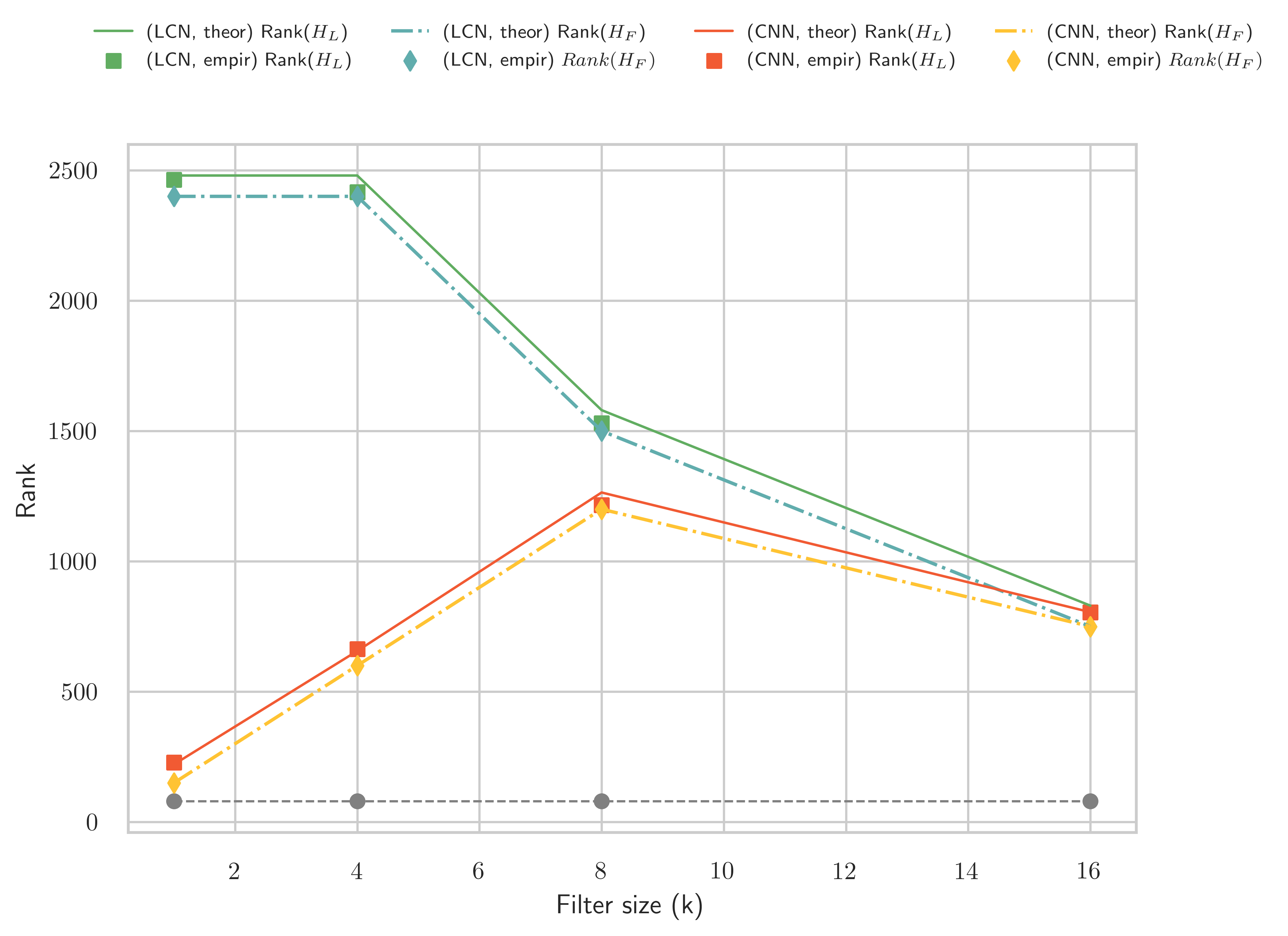
Figure 3: Hessian rank: LCN vs CNN, (Linear, CIFAR10).

8 Conclusion

All in all, we have illustrated how the key ingredients of CNNs, such as local connectivity and weight sharing, as well as architectural aspects like filter size, strides, and number of channels get manifested through the Hessian structure and rank. Moreover, we can utilize our Toeplitz representation framework to deliver tight upper bounds in the general case of deep convolutional networks and generalize the recent finding of (Singh et al., 2021) about square root growth of rank relative to parameter count for CNNs as well. Looking ahead, our work raises some very interesting questions: (a) Is the growth of rank as a square root in terms of the number of parameters a universal characteristic of all deep architectures? Including Transformers? Or are there some exceptions to it? (b) Given the uncovered structure of the Hessian in CNNs, there are also questions about understanding which parts of the architecture affect the spectrum more — normalization or pooling layers? (c) On the application side, it would be interesting to see if we can use our results to understand the approximation quality of existing pre-conditioners such as K-FAC or come up with better ones, given the rich properties of Toeplitz matrices.

Appendix A Tools

A.1 Toeplitz Derivative

Lemma 1.

The matrix derivative of ${{\bf T}}^{(l)}$ with respect to $\mathbf{W}^{(l)}$, is given as follows:

$$\dfrac{\partial{{\bf T}}^{(l)}}{\partial\mathbf{W}^{(l)}}:=\dfrac{\partial\operatorname{vec}_{r}{{\bf T}}^{(l)}}{\partial\left(\operatorname{vec}_{r}\mathbf{W}^{(l)}\right)^{\top}}={\bf I}_{m_{l}}\,\mathbin{\mathop{\otimes}}\,{{\bf Q}}^{(l)}\,,$$

which lives in ${\mathbb{R}^{m_{l}\,m_{l-1}\,d_{\ell}\,d_{l-1}\times m_{l}\,m_{l-1}\,k_{l}}}$, and the matrix ${{\bf Q}}^{(l)}\in{\mathbb{R}^{m_{l-1}d_{l}d_{l-1}\times m_{l-1}k_{l}}}$ is defined as:

$${{\bf Q}}^{(l)}:=\begin{pmatrix}{\bf I}_{m_{l-1}}\mathbin{\mathop{\otimes}}\left(\pi_{R}^{0}\,{\bf I}_{d_{l-1}\times k_{l}}\right)\\[2.84526pt] \vdots\\[2.84526pt] {\bf I}_{m_{l-1}}\mathbin{\mathop{\otimes}}\left(\pi_{R}^{d_{l-1}-k_{l}}\,{\bf I}_{d_{l-1}\times k_{l}}\right)\\[2.84526pt] \end{pmatrix}$$

where $\pi_{R}$ is the permutation matrix performs clockwise rotation of the rows of the matrix it is left-multiplied with, and its superscript the matrix power (so, $\pi_{R}^{0}={\bf I}_{d_{l-1}})$. Also, in the above expression ${\bf I}_{d_{l-1}\times k_{l}}$ is the ‘tall’ identity matrix, i.e., $[{\bf I}_{k_{l}},\bm{0}]^{\top}$ (as $k_{l}\leq d_{l-1}$).

Proof.

It is quite clear that the non-zero parts in the derivative will arise only when compute the derivative of Toeplitz of one row with respect to the elements of the same row. In other words, only when considering:

$$\dfrac{\partial{{\bf T}}^{{\mathcal{W}^{(l)}_{(i,j)\,\bullet}}}}{\partial{\mathcal{W}^{(l)}_{(r,s)\,\bullet}}}\quad\quad\text{for}\;i=r,\;\;j=s\,.$$

And rest of the blocks will be zeros. This explains the occurrence of two Kronecker products, with respect to ${\bf I}_{m_{l}}$ and ${\bf I}_{m_{l-1}}$.

More concretely, recall that:

$${{{\bf T}}^{(l)}:=\begin{pmatrix}{{\bf T}}^{{\mathcal{W}^{(l)}_{(1,1)\,\bullet}}}&\cdots&{{\bf T}}^{{\mathcal{W}^{(l)}_{(1,m_{l-1})\,\bullet}}}\\[2.84526pt] \vdots&&\vdots\\[2.84526pt] {{\bf T}}^{{\mathcal{W}^{(l)}_{(m_{l},1)\,\bullet}}}&\cdots&{{\bf T}}^{{\mathcal{W}^{(l)}_{(m_{l},m_{l-1})\,\bullet}}}\\[2.84526pt] \end{pmatrix}\,,}\quad\text{and}$$

$${{\bf W}}^{(l)}:=\operatorname{mat}{{\mathcal{W}}^{(l)}}:=\begin{pmatrix}{{\mathcal{W}^{(l)}_{(1,1)\,\bullet}}}&\cdots&{{\mathcal{W}^{(l)}_{(m_{l},1)\,\bullet}}}\\ \vdots&&\vdots\\ {{\mathcal{W}^{(l)}_{(1,m_{l-1})\,\bullet}}}&\cdots&{{\mathcal{W}^{(l)}_{(m_{l},m_{l-1})\,\bullet}}}\\ \end{pmatrix}^{\top}=\begin{pmatrix}w_{1,1,1}&\cdots&w_{1,1,k_{l}}&\cdots&w_{1,m_{l-1},1}&\cdots&w_{1,m_{l-1},k_{l}}\\ \vdots&&\vdots&&\vdots&&\vdots\\ w_{m_{l},1,1}&\cdots&w_{m_{l},1,k_{l}}&\cdots&w_{m_{l},m_{l-1},1}&\cdots&w_{m_{l},m_{l-1},k_{l}}\\ \end{pmatrix}\,.$$ (9)

Let’s use the shorthand ${{\bf T}}^{(l)}_{(i,\bullet)}:=\begin{pmatrix}{{\bf T}}^{{\mathcal{W}^{(l)}_{(i,1)\,\bullet}}}&\cdots&{{\bf T}}^{{\mathcal{W}^{(l)}_{(i,m_{l-1})\,\bullet}}}\\ \end{pmatrix}$. Now, the general structure of the required Toeplitz derivative has the following form:

code-for-first-row = , code-for-first-col = ,

(10)

(11)

(12)

(13)

(14)

Thediagonal

References

- Amari (1998) Amari, S.-I. Natural gradient works efficiently in learning. Neural computation, 10(2):251–276, 1998.
- Belkin et al. (2019) Belkin, M., Hsu, D., Ma, S., and Mandal, S. Reconciling modern machine learning practice and the bias-variance trade-off, 2019.
- Bruna & Mallat (2013) Bruna, J. and Mallat, S. Invariant scattering convolution networks. IEEE transactions on pattern analysis and machine intelligence, 35(8):1872–1886, 2013.
- Chuai & Tian (2004) Chuai, J. and Tian, Y. Rank equalities and inequalities for kronecker products of matrices with applications. Applied Mathematics and Computation, 150(1):129–137, 2004. ISSN 0096-3003. doi: https://doi.org/10.1016/S0096-3003(03)00203-0. URL https://www.sciencedirect.com/science/article/pii/S0096300303002030.
- Cohen et al. (2021) Cohen, J. M., Kaur, S., Li, Y., Kolter, J. Z., and Talwalkar, A. Gradient descent on neural networks typically occurs at the edge of stability, 2021. URL https://arxiv.org/abs/2103.00065.
- Cohen & Shashua (2016) Cohen, N. and Shashua, A. Inductive bias of deep convolutional networks through pooling geometry. arXiv preprint arXiv:1605.06743, 2016.
- Dauphin et al. (2014) Dauphin, Y. N., Pascanu, R., Gulcehre, C., Cho, K., Ganguli, S., and Bengio, Y. Identifying and attacking the saddle point problem in high-dimensional non-convex optimization. Advances in neural information processing systems, 27, 2014.
- Dosovitskiy et al. (2020) Dosovitskiy, A., Beyer, L., Kolesnikov, A., Weissenborn, D., Zhai, X., Unterthiner, T., Dehghani, M., Minderer, M., Heigold, G., Gelly, S., et al. An image is worth 16x16 words: Transformers for image recognition at scale. arXiv preprint arXiv:2010.11929, 2020.
- Fang et al. (2020) Fang, Z., Feng, H., Huang, S., and Zhou, D.-X. Theory of deep convolutional neural networks ii: Spherical analysis. Neural Networks, 131:154–162, 2020.
- Fukushima (1980) Fukushima, K. A self-organizing neural network model for a mechanism of pattern recognition unaffected by shift in position. Biol, Cybern, 36:193–202, 1980.
- Garriga-Alonso et al. (2018) Garriga-Alonso, A., Rasmussen, C. E., and Aitchison, L. Deep convolutional networks as shallow gaussian processes. arXiv preprint arXiv:1808.05587, 2018.
- Ghorbani et al. (2019) Ghorbani, B., Krishnan, S., and Xiao, Y. An investigation into neural net optimization via hessian eigenvalue density. In International Conference on Machine Learning, pp. 2232–2241. PMLR, 2019.
- Gu et al. (2020) Gu, Y., Zhang, W., Fang, C., Lee, J. D., and Zhang, T. How to characterize the landscape of overparameterized convolutional neural networks. Advances in Neural Information Processing Systems, 33:3797–3807, 2020.
- Gull (1989) Gull, S. F. Developments in Maximum Entropy Data Analysis, pp. 53–71. Springer Netherlands, Dordrecht, 1989. ISBN 978-94-015-7860-8. doi: 10.1007/978-94-015-7860-8_4. URL https://doi.org/10.1007/978-94-015-7860-8_4.
- Gunasekar et al. (2018) Gunasekar, S., Woodworth, B., Bhojanapalli, S., Neyshabur, B., and Srebro, N. Implicit regularization in matrix factorization. In 2018 Information Theory and Applications Workshop (ITA), pp. 1–10. IEEE, 2018.
- Gur-Ari et al. (2018) Gur-Ari, G., Roberts, D. A., and Dyer, E. Gradient descent happens in a tiny subspace, 2018.
- Hassibi & Stork (1992) Hassibi, B. and Stork, D. G. Second order derivatives for network pruning: Optimal brain surgeon. In NIPS, pp. 164–171, 1992. URL http://papers.nips.cc/paper/647-second-order-derivatives-for-network-pruning-optimal-brain-surgeon.
- Hochreiter & Schmidhuber (1997) Hochreiter, S. and Schmidhuber, J. Flat minima. Neural computation, 9(1):1–42, 1997.
- Jacot et al. (2018) Jacot, A., Gabriel, F., and Hongler, C. Neural tangent kernel: Convergence and generalization in neural networks. arXiv preprint arXiv:1806.07572, 2018.
- Jia & Su (2020) Jia, Z. and Su, H. Information-theoretic local minima characterization and regularization. In International Conference on Machine Learning, pp. 4773–4783. PMLR, 2020.
- Jiang et al. (2019) Jiang, Y., Neyshabur, B., Mobahi, H., Krishnan, D., and Bengio, S. Fantastic generalization measures and where to find them. arXiv preprint arXiv:1912.02178, 2019.
- Keskar et al. (2016) Keskar, N. S., Mudigere, D., Nocedal, J., Smelyanskiy, M., and Tang, P. T. P. On large-batch training for deep learning: Generalization gap and sharp minima. arXiv preprint arXiv:1609.04836, 2016.
- Kiranyaz et al. (2021) Kiranyaz, S., Avci, O., Abdeljaber, O., Ince, T., Gabbouj, M., and Inman, D. J. 1d convolutional neural networks and applications: A survey. Mechanical systems and signal processing, 151:107398, 2021.
- Kirkpatrick et al. (2017) Kirkpatrick, J., Pascanu, R., Rabinowitz, N., Veness, J., Desjardins, G., Rusu, A. A., Milan, K., Quan, J., Ramalho, T., Grabska-Barwinska, A., et al. Overcoming catastrophic forgetting in neural networks. Proceedings of the national academy of sciences, 114(13):3521–3526, 2017.
- Kohn et al. (2021) Kohn, K., Merkh, T., Montúfar, G., and Trager, M. Geometry of linear convolutional networks, 2021. URL https://arxiv.org/abs/2108.01538.
- Krizhevsky et al. (2017) Krizhevsky, A., Sutskever, I., and Hinton, G. E. Imagenet classification with deep convolutional neural networks. Communications of the ACM, 60(6):84–90, 2017.
- Kunstner et al. (2019) Kunstner, F., Hennig, P., and Balles, L. Limitations of the empirical fisher approximation for natural gradient descent. Advances in neural information processing systems, 32, 2019.
- LeCun et al. (1990) LeCun, Y., Denker, J. S., and Solla, S. A. Optimal brain damage. In Advances in neural information processing systems, pp. 598–605, 1990.
- LeCun et al. (1992) LeCun, Y., Simard, P., and Pearlmutter, B. A. Automatic learning rate maximization by on-line estimation of the hessian’s eigenvectors. In NIPS 1992, 1992.
- LeCun et al. (1995) LeCun, Y., Bengio, Y., et al. Convolutional networks for images, speech, and time series. The handbook of brain theory and neural networks, 3361(10):1995, 1995.
- Liu et al. (2021) Liu, Z., Lin, Y., Cao, Y., Hu, H., Wei, Y., Zhang, Z., Lin, S., and Guo, B. Swin transformer: Hierarchical vision transformer using shifted windows. In Proceedings of the IEEE/CVF international conference on computer vision, pp. 10012–10022, 2021.
- Liu et al. (2022) Liu, Z., Mao, H., Wu, C.-Y., Feichtenhofer, C., Darrell, T., and Xie, S. A convnet for the 2020s. In Proceedings of the IEEE/CVF Conference on Computer Vision and Pattern Recognition, pp. 11976–11986, 2022.
- MacKay (1992a) MacKay, D. J. A practical bayesian framework for backpropagation networks. Neural computation, 4(3):448–472, 1992a.
- MacKay (1992b) MacKay, D. J. C. A Practical Bayesian Framework for Backpropagation Networks. Neural Computation, 4(3):448–472, 05 1992b. ISSN 0899-7667. doi: 10.1162/neco.1992.4.3.448. URL https://doi.org/10.1162/neco.1992.4.3.448.
- Maddox et al. (2020) Maddox, W. J., Benton, G., and Wilson, A. G. Rethinking parameter counting: Effective dimensionality revisted. arXiv preprint arXiv:2003.02139, 2020.
- Magnus & Neudecker (2019) Magnus, J. R. and Neudecker, H. Matrix differential calculus with applications in statistics and econometrics. John Wiley & Sons, 2019.
- Mao et al. (2021) Mao, T., Shi, Z., and Zhou, D.-X. Theory of deep convolutional neural networks iii: Approximating radial functions, 2021. URL https://arxiv.org/abs/2107.00896.
- Martens & Grosse (2015) Martens, J. and Grosse, R. B. Optimizing neural networks with kronecker-factored approximate curvature. CoRR, abs/1503.05671, 2015. URL http://arxiv.org/abs/1503.05671.
- Matsaglia & Styan (1974) Matsaglia, G. and Styan, G. P. H. Equalities and inequalities for ranks of matrices. Linear and Multilinear Algebra, 2(3):269–292, 1974. doi: 10.1080/03081087408817070. URL https://doi.org/10.1080/03081087408817070.
- Nguyen & Hein (2018) Nguyen, Q. and Hein, M. Optimization landscape and expressivity of deep cnns. In International conference on machine learning, pp. 3730–3739. PMLR, 2018.
- Papyan (2020) Papyan, V. Traces of class/cross-class structure pervade deep learning spectra. The Journal of Machine Learning Research, 21(1):10197–10260, 2020.
- Pennington & Bahri (2017) Pennington, J. and Bahri, Y. Geometry of neural network loss surfaces via random matrix theory. In Precup, D. and Teh, Y. W. (eds.), Proceedings of the 34th International Conference on Machine Learning, volume 70 of Proceedings of Machine Learning Research, pp. 2798–2806. PMLR, 06–11 Aug 2017. URL http://proceedings.mlr.press/v70/pennington17a.html.
- Poggio et al. (2015) Poggio, T., Anselmi, F., and Rosasco, L. I-theory on depth vs width: hierarchical function composition. Technical report, Center for Brains, Minds and Machines (CBMM), 2015.
- Sagun et al. (2016) Sagun, L., Bottou, L., and LeCun, Y. Eigenvalues of the hessian in deep learning: Singularity and beyond. arXiv preprint arXiv:1611.07476, 2016.
- Sagun et al. (2017) Sagun, L., Evci, U., Guney, V. U., Dauphin, Y., and Bottou, L. Empirical analysis of the hessian of over-parametrized neural networks. arXiv preprint arXiv:1706.04454, 2017.
- Schaul et al. (2013) Schaul, T., Zhang, S., and LeCun, Y. No more pesky learning rates, 2013.
- Schraudolph (2002a) Schraudolph, N. N. Fast curvature matrix-vector products for second-order gradient descent. Neural Computation, 14:1723–1738, 2002a.
- Schraudolph (2002b) Schraudolph, N. N. Fast curvature matrix-vector products for second-order gradient descent. Neural computation, 14(7):1723–1738, 2002b.
- Sedghi et al. (2018) Sedghi, H., Gupta, V., and Long, P. M. The singular values of convolutional layers, 2018.
- Setiono & Hui (1995) Setiono, R. and Hui, L. C. K. Use of a quasi-newton method in a feedforward neural network construction algorithm. IEEE Transactions on Neural Networks, 6(1):273–277, 1995.
- Singh (1972) Singh, R. P. Some generalizations in matrix differentiation with applications in multivariate analysis. 1972.
- Singh & Alistarh (2020) Singh, S. P. and Alistarh, D. Woodfisher: Efficient second-order approximation for neural network compression, 2020.
- Singh et al. (2021) Singh, S. P., Bachmann, G., and Hofmann, T. Analytic insights into structure and rank of neural network hessian maps. Advances in Neural Information Processing Systems, 34, 2021.
- Singh et al. (2022) Singh, S. P., Lucchi, A., Hofmann, T., and Schölkopf, B. Phenomenology of double descent in finite-width neural networks. In International Conference on Learning Representations, 2022. URL https://openreview.net/forum?id=lTqGXfn9Tv.
- Tolstikhin et al. (2021) Tolstikhin, I. O., Houlsby, N., Kolesnikov, A., Beyer, L., Zhai, X., Unterthiner, T., Yung, J., Steiner, A., Keysers, D., Uszkoreit, J., et al. Mlp-mixer: An all-mlp architecture for vision. Advances in Neural Information Processing Systems, 34:24261–24272, 2021.
- Tracy & Dwyer (1969) Tracy, D. S. and Dwyer, P. S. Multivariate maxima and minima with matrix derivatives. Journal of the American Statistical Association, 64(328):1576–1594, 1969.
- Vapnik (1991) Vapnik, V. Principles of risk minimization for learning theory. Advances in neural information processing systems, 4, 1991.
- Vaswani et al. (2017) Vaswani, A., Shazeer, N., Parmar, N., Uszkoreit, J., Jones, L., Gomez, A. N., Kaiser, Ł., and Polosukhin, I. Attention is all you need. Advances in neural information processing systems, 30, 2017.
- Wu et al. (2020) Wu, Y., Zhu, X., Wu, C., Wang, A., and Ge, R. Dissecting hessian: Understanding common structure of hessian in neural networks. arXiv preprint arXiv:2010.04261, 2020.
- Yang et al. (2019) Yang, J., Sun, S., and Roy, D. M. Fast-rate pac-bayes generalization bounds via shifted rademacher processes, 2019.
- Yao et al. (2020) Yao, Z., Gholami, A., Keutzer, K., and Mahoney, M. W. Pyhessian: Neural networks through the lens of the hessian. In 2020 IEEE international conference on big data (Big data), pp. 581–590. IEEE, 2020.
- Zhao et al. (2017) Zhao, L., Liao, S., Wang, Y., Li, Z., Tang, J., and Yuan, B. Theoretical properties for neural networks with weight matrices of low displacement rank. In international conference on machine learning, pp. 4082–4090. PMLR, 2017.
- Zhu et al. (1997) Zhu, C., Byrd, R. H., Lu, P., and Nocedal, J. Algorithm 778: L-bfgs-b: Fortran subroutines for large-scale bound-constrained optimization. ACM Transactions on Mathematical Software (TOMS), 23(4):550–560, 1997.