Interplay between Topology and Edge Weights in Real-World Graphs: Concepts, Patterns, and an Algorithm

Abstract

What are the relations between the edge weights and the topology in real-world graphs? Given only the topology of a graph, how can we assign realistic weights to its edges based on the relations? Several trials have been done for edge-weight prediction where some unknown edge weights are predicted with most edge weights known. There are also existing works on generating both topology and edge weights of weighted graphs. Differently, we are interested in generating edge weights that are realistic in a macroscopic scope, merely from the topology, which is unexplored and challenging. To this end, we explore and exploit the patterns involving edge weights and topology in real-world graphs. Specifically, we divide each graph into layers where each layer consists of the edges with weights at least a threshold. We observe consistent and surprising patterns appearing in multiple layers: the similarity between being adjacent and having high weights, and the nearly-linear growth of the fraction of edges having high weights with the number of common neighbors. We also observe a power-law pattern that connects the layers. Based on the observations, we propose PEAR, an algorithm assigning realistic edge weights to a given topology. The algorithm relies on only two parameters, preserves all the observed patterns, and produces more realistic weights than the baseline methods with more parameters.

1 Introduction

In weighted graphs, the edge weights reveal the heterogeneity of edges and enrich the information provided by the topology (Newman, 2004). In practice, weighted graphs have been widely used to model traffic (De Montis et al., 2007), biological interactions (Aittokallio and Schwikowski, 2006), personal preference (Liu et al., 2009), etc. The relation between topology and edge weights, therefore, attracts much attention. A typical scenario where the two kinds of information are integrated is edge-weight prediction (Fu et al., 2018; Rotabi et al., 2017). The target of edge-weight prediction is to predict the unknown edge weights using the given topological and edge-weight information, where usually most of the edge weights are given as the inputs. Another related direction is to generate both the topology and the edge weights of weighted graphs (Akoglu et al., 2008; McGlohon et al., 2008; Yang et al., 2021).

However, not much has been explored about the relation between the pure topology and the edge weights in a graph, despite the importance of the relation. In some previous trials, the problem of classifying edges into strong ones and weak ones by assuming strong triadic closure (Sintos and Tsaparas, 2014) (STC) is considered. The STC assumption forbids open triangles (also called triads or wedges) with two strong edges and aims to maximize the number of strong edges. However, the diversity of edge weights is over-simplified in such a setting. Moreover, it has been pointed out by Adriaens et al. (2020) that the STC assumption with a maximum number of strong edges is often far from reality. The generalized version considered by Adriaens et al. (2020) still has room for improvement, especially w.r.t the empirical grounds, as shown in the experimental results.

Specifically, we study how the edge weights in real-world graphs are related to the topology in a macroscopic way, which allows us to generate realistic edge weights when given an unweighted topology. We would like to emphasize that we do not aim to assign edge weights with small errors w.r.t each individual edge. We are motivated by the following practical applications:

• Edge weight anonymization. In social networks, due to data privacy issues, sometimes only the binary connections are publicly accessible, while the detailed edge weights should not be publicized (Steinhaeuser and Chawla, 2008; Skarkala et al., 2012). Using the macroscopic patterns, we are able to generate realistic edge weights for a given topology and publicize the generated weighted graph to researchers and practitioners as a benchmark dataset, without revealing the true edge weights.

• Anomaly detection. In communication networks, the edge weights usually represent the frequency or intensity of the communication between the entities. Using the patterns observed on real-world graphs, we may detect anomalous edge weights that deviate from the patterns, and they may correspond to entities that have abnormally frequent or intensive communication (Thottan et al., 2010; Akoglu et al., 2015).

• Community detection. Community detection is a fundamental problem in network analysis (Fortunato, 2010). Edge weights are known to be helpful for community detection because they provide additional information about the strength and importance of connections between nodes (Liu et al., 2014; He et al., 2021), and thus assigning edge weights to unweighted graphs has the potential to enhance the performance of community detection algorithms (Berry et al., 2011).

We introduce and use a new tool called layers to study weighted graphs in a hierarchical way, where each layer is a subgraph that consists of the edges with weights exceeding some threshold. We examine eleven real-world graphs from five different domains and observe consistently strong correlations between the number of common neighbors (CNs) of an edge and the weight of the edge. Although the information of CNs has been widely used in link prediction (Wang et al., 2015) and used to indicate the significance of individual edges (Ahmad et al., 2020; Cao et al., 2015; Zhu and Xia, 2016), to the best of our knowledge, we are the first to study the quantitative patterns between the information of CNs and edge weights in a macroscopic scope. We observe consistent within-layer patterns in multiple layers: (1) the nearly-linear growth of fraction of high-weight edges with the number of CNs, (2) the relation between being adjacent and having high weights (specifically, the relation between the fraction of high-weight edges and that of adjacent pairs with the same name number of CNs), and across the layers, we observe a power-law correlation between the overall fraction of high-weight edges and the counterpart within the group of edges sharing no CNs. Based on the observations, we propose PEAR (Pattern-based Edge-weight Assignment on gRaphs), an algorithm for assigning realistic edge weights to a given topology by preserving all the observed macroscopic patterns. The proposed algorithm has only two parameters. On multiple real-world datasets, PEAR outperforms the baseline methods using the same number of, or even more, parameters, producing more realistic edge weights in several different aspects w.r.t different macroscopic network statistics.

In short, our contributions are five-fold:

• New problem. We introduce a new challenging problem: realistic assignment of edge weights merely based on topology.

• New perspective. We introduce the concept of layers, which provides a new perspective to study weighted graphs.

• Patterns. We extensively study eleven real-world graphs and discover the various relations between topology and edge weights.

• Algorithm. We propose PEAR, a weight-assignment algorithm based on the observed patterns. The algorithm has only two parameters yet produces realistic edge weights to a given topology.

• Experiments. We evaluate PEAR on real-world graphs. Without sophisticated fine-tuning, PEAR overall outperforms the baseline methods with more parameters, producing more realistic edge-weights w.r.t node-degree and edge-CN distributions, average clustering coefficient, and a graph distance measure computed by NetSimile (Berlingerio et al., 2012).

Roadmap.whiteRoadmap. The remaining part of the paper is organized as follows. In Section 2, we discuss related work. In Section 3, we provide some preliminaries. In Section 4, we propose some new concepts. In Section 5, we describe the patterns that we observe on real-world datasets. In Section 6, we formulate our observations and, based on them, propose our algorithm, PEAR. In Section 7, the empirical evaluation of PEAR on real-world datasets is demonstrated. In Section 8, we discuss some potential limitations of our work and future directions, and lastly, conclude the paper.

Reproducibility.whiteReproducibility. The code and datasets are available online (Bu et al., 2022).

2 Related work

Edge-weight prediction.whiteEdge-weight prediction. In the early trials of edge-weight prediction (Aicher et al., 2015; Zhao et al., 2015; Zhu et al., 2016), the problem is dealt with as a natural extension of the link prediction (Martínez et al., 2016) problem. Specifically, the proposed link-prediction algorithms assign scores to node pairs as the likelihood of edge existence, and the scores are also naturally used as the estimated edge weights. More recently, Fu et al. (2018) use multiple topological features to predict the unknown edge weights in a supervised manner. Specifically, they fit a regression model to the known edge weights with the features and use the fitted model to predict the unknown ones. The main differences between the problem that we focus on in this work and the edge-weight prediction problem are: (1) in the edge-weight prediction problem, most (e.g., 80% (Aicher et al., 2015) or 90% (Fu et al., 2018; Zhao et al., 2015; Zhu et al., 2016)) of the edge weights are assumed to be known and are given together with topology as the inputs, while we consider the scenarios where we only have access to the topology and we have none known edge weights; and (2) the target of the edge-weight prediction problem is to estimate the weights of individual edges in a microscopic way, while we aim to generate realistic edge weights for a given topology preserving the macroscopic patterns that we observe in real-world graphs. Notably, there is another independent research problem that focuses on the edge-weight prediction of weighted signed graphs, which has essential differences from the research problem in this paper. Specifically, the techniques proposed in a recent work studying that problem (Kumar et al., 2016) are specially designed for weighted signed graphs representing pairwise relations such as like/dislike and trust/distrust, which cannot be directly applied to the scenarios that we focus on where the edge weights represent the repetitions of the corresponding binary relations.

Weighted-graph generation.whiteWeighted-graph generation. The other trials exploring the interplay between topology and edge weights, include the weighted-graph generation problem (Akoglu et al., 2008; McGlohon et al., 2008; Yang et al., 2021). In those works, the authors specifically study the evolution of both topology and edge weights over time, and they propose algorithms that generate both topology and edge weights of weighted graphs. Although some simple static patterns (e.g., power-law or geometric weight distributions) are also discussed in those works, the problem that we focus on, generating edge weights for a given topology, is essentially and technically different with the weighted-graph generation problem since in our problem the topology is given and thus fixed.

Strong triadic closure.whiteStrong triadic closure. The concept of strong triadic closure (STC) is first proposed by Sintos and Tsaparas (2014), where the authors consider the problem of classifying edges into strong ones and weak ones. They define that a graph satisfies the STC property if there exists no open triangle with two strong edges, and they assume that graphs often satisfy the STC property and have many strong edges. Therefore, they specifically consider the problem of maximizing the number of strong edges while satisfying the STC property. However, only two types of edge weights are considered in this problem, while real-world graphs often have a high diversity of edge weights (see, e.g., the datasets in Table 2). Moreover, this optimization problem has both theoretical (it can have many optimal solutions) and practical (real-world graphs often do not have many strong edges) limitations, as pointed out by Adriaens et al. (2020). Even though the above problem has been extended to edge weights of a wider range with other modifications (Adriaens et al., 2020), the extended version still has room for improvement w.r.t the empirical grounds, and the methods fail to predict the edge weights of real-world graphs accurately. Specifically, the predicted edge weights have almost zero correlation with the ground truth on many datasets, as shown by Adriaens et al. (2020).

To the best of our knowledge, we are the first to consider the problem of assigning realistic edge weights to a given topology by trying to preserve patterns observed on real-world graphs.

3 Preliminaries

In this section, we provide some mathematical and notational backgrounds.

A weighted graph $G=(V,E,W)$ consists of a node set $V=V(G)$, an edge set $E=E(G)\in\binom{V}{2}$, and edge weights $W=W(G)$. By ignoring the edge weights, we have the underlying unweighted graph $\mkern 1.5mu\overline{\mkern-1.5muG\mkern-1.5mu}\mkern 1.5mu=(V,E)$ of $G$. For each edge $e\in E$, $W_{e}$ is the weight of $e$. In this work, we focus on graphs with positive integer edge weights, i.e., $W\in\mathbb{N}^{E}$, where $\mathbb{N}$ is the set of positive integers, where each edge weight represents the number of occurrences of the corresponding edge. Note that the analysis on weighted graphs is mainly done on the graphs with integer edge weights (Newman, 2004), and for graphs with non-integer edge weights, we may round each edge weight to the nearest integer. All graphs are assumed to be undirected and without self-loops. Thus, $(u,v)$ and $(v,u)$ represent the same edge (i.e., the set $\{u,v\}$) between two nodes $u\neq v\in V$.

The concepts below use only the topology of $G$ (i.e., $V$ and $E$). For each node $v\in V$, $N_{v}(G)=\{v^{\prime}\in V:(v,v^{\prime})\in E\}$ is the neighborhood of $v$ in $G$, and $d_{v}(G)=|N_{v}(G)|$ is the degree of $v$ in $G$. For two nodes $u,v\in V$, $CN_{uv}(G)=N_{u}(G)\cap N_{v}(G)$ is the set of common neighbors (CNs) of $u$ and $v$ in $G$, and we say the two nodes $u$ and $v$ share the common neighbors in $CN_{uv}(G)$. For an edge $e=(u,v)$, we use $CN_{e}(G)$ to denote $CN_{uv}(G)$, and we say that the edge $e$ shares the common neighbors in $CN_{e}(G)$. Sometimes, the number $|CN_{e}(G)|$ of common neighbors shared by the two endpoints of $e$ is called the embeddedness (Cleaver, 2002) of $e$.

Given $G=(V,E,W)$, the line graph (Harary and Norman, 1960) of $G$ is the graph $L(G)=(E,X)$, where the nodes of $L(G)$ one-to-one correspond to the edges of $G$ and two nodes of $L(G)$ are adjacent to each other if and only if the two corresponding edges in $G$ share a common endpoint. Given $k\in\mathbb{N}$, the $k$-core (Seidman, 1983) $C_{k}(G)$ of $G$ is the maximal subgraph of $G$ where each node of $C_{k}(G)$ has degree $k$ within it.

Table 1: Notations and abbreviations.

Notation/Abbreviation	Definition/Meaning
$G=(V,E,W)$	a graph with a node set $V$, a edge set $E$, and edge weights $W$
$\mkern 1.5mu\overline{\mkern-1.5muG\mkern-1.5mu}\mkern 1.5mu=(V,E)$	the underlying unweighted graph of $G$
$W_{e}$	the edge weight of $e\in E$
$N_{v}(G)$	the set of neighbors of $v\in V$
$d_{v}(G)$	the degree of $v\in V$
$CN_{uv}(G)$	the set of common neighbors of $u,v\in V$
$G_{i}=(V_{i},E_{i},W_{i})$	the layer-$i$ of $G$ whose edge set consists of the edges with weights $\geq i$ in $G$
$R_{i}=\binom{V_{i}}{2}$	the set of all the node pairs in $G_{i}$
$E_{c;i}(G)$	the set of edges sharing $c$ common neighbors in $G_{i}$
$R_{c;i}(G)$	the set of pairs sharing $c$ common neighbors in $G_{i}$
$f_{overall;i}(G)$ ($\tilde{f}_{overall;i}(G)$)	the overall fraction of weighty edges (adjacent pairs) w.r.t $G$ and $i$ (Def. 2)
$f_{c;i}(G)$ ($\tilde{f}_{c;i}(G)$)	the fraction of weighty edges (adjacent pairs) within $E_{c;i}(G)$ (Def. 2)
CN	common neighbor
PEAR	Pattern-based Edge-weight Assignment on gRaphs
FoWE	fraction of weighty edges
FoAP	fraction of adjacent pairs

We list the frequently used notations and abbreviations in Table 1. In the notations, the input graph $G$ can be omitted when the context is clear.

In this paper, we consider the problem where given the topology of a graph, we aim to assign realistic edge weights to the topology based on several patterns observed on real-world graphs, where each edge weight is a positive integer representing the number of occurrences of the corresponding edge. We formulate the considered problem (informally at this moment) as follows:

Problem 1 (Informal).

Given an unweighted graph $\mkern 1.5mu\overline{\mkern-1.5muG\mkern-1.5mu}\mkern 1.5mu=(V,E)$, we aim to generate edge weights $W:E\rightarrow\mathbb{N}$ that satisfy a group of realistic properties regarding the interplay between topology and edge weights, where each edge weight is a positive integer representing the number of occurrences of the corresponding edge.

We shall first present the patterns (i.e., the group of realistic properties) that we observe on real-world graphs, and then we provide a formal problem statement by formulating the patterns as mathematical properties. Finally, we propose an algorithm that assigns realistic edge weights to a given topology while preserving the formulated properties.

4 Proposed concepts

In this section, we introduce the proposed concepts. We will use them to describe our observations and design our algorithm.

When given an unweighted graph $\mkern 1.5mu\overline{\mkern-1.5muG\mkern-1.5mu}\mkern 1.5mu=(V,E)$, the topology divides the pairs $\binom{V}{2}$ of nodes into two categories. Each pair $(u,v)\in\binom{V}{2}$ of nodes is either adjacent ($(u,v)\in E$, weight $\geq 1$) or distant ($(u,v)\notin E$, weight $<1$). When we have a weighted graph $G=(V,E,W)$, we can similarly set different weight thresholds $i\in\mathbb{N}$ and extract the subgraph consisting of edges with weight $\geq i$, which gives the following definition of layers.

Definition 1 (Layers).

Given $G=(V,E,W)$ and $i\in N$, the layer-$i$ of $G$ is the weighted graph $G_{i}=(V_{i},E_{i},W_{i})$ obtained from $G$ by taking the edges with weights greater than or equal to $i$. Formally, $E_{i}=E_{i}(G)=\{e\in E:W_{e}\geq i\}$, and $W_{i}=W_{i}(G)$ satisfies that $W_{i}(e)=W(e),\forall e\in E_{i}$. We also define all the possible node pairs $R_{i}=R_{i}(G)=\binom{V_{i}}{2}$.

Based on the concept of layers, we also define the following related concepts, weighty edges (WEs) and fraction of weighty edges (FoWE), w.r.t each layer of a graph. Intuitively, in each layer, the weighty edges are the edges with weights higher than the threshold determined by the layer. Notably, we define overall FoWEs for the whole layer, and we also define FoWE w.r.t each number $c$ of common neighbors (CNs).

Definition 2 (Fractions of weighty edges and adjacent pairs).

Given $G=(V,E,W)$ and $i\in\mathbb{N}$, we call an edge $e\in E_{i}$ a weighty edge (w.r.t $G$ and $i$) if and only if $W_{e}>i$ (i.e., $e\in E_{i+1}$), where recall that $E_{i}$ is the edge set of $G_{i}$. The overall fraction of weighty edges $f_{overall;i}(G)$ is defined as $|E_{i+1}|/|E_{i}|$. Further given $c\in\mathbb{N}$, let $E_{c;i}\subseteq E_{i}$ denote the set of edges sharing $c$ CNs (i.e., edges whose endpoints share $c$ CNs) in $G_{i}$. The fraction of weighty edges (w.r.t $G$, $i$, and $c$) $f_{c;i}(G)$ is defined as $|E_{c;i}\cap E_{i+1}|/|E_{c;i}|$. Similarly, we define the overall fraction of adjacent pairs $\tilde{f}_{overall;i}(G)=|E_{i}|/|R_{i}|$, as well as the fraction of adjacent pairs (w.r.t $G$, $i$, and $c$) $\tilde{f}_{c;i}(G)=|E_{c;i}|/|R_{c;i}|$ for each $c$, where $R_{c;i}$ is the set of pairs sharing $c$ CNs in $G_{i}$.

Table 2: Some basic statistics (number of nodes and number of edges in each of the first four layers) of the eleven real-world datasets (Opsahl, 2013; Benson et al., 2018; Paranjape et al., 2017; Sinha et al., 2015) from five domains used in our empirical study. The datasets are grouped w.r.t their domains.

dataset	$|V|$	$|E|=|E_{1}|$	$|E_{2}|$	$|E_{3}|$	$|E_{4}|$
OF	897	71,380	47,266 (66.2$\%$)	35,456 (49.7$\%$)	28,546 (40.0$\%$)
FL	2,905	15,645	4,608 (29.5$\%$)	1,507 (9.6$\%$)	564 (3.6$\%$)
th-UB	82,075	182,648	7,297 (4.0$\%$)	2,090 (1.1$\%$)	965 (0.5$\%$)
th-MA	152,702	1,088,735	128,400 (11.8$\%$)	48,605 (4.5$\%$)	26,121 (2.4$\%$)
th-SO	2,301,070	20,989,078	1,168,210 (5.6$\%$)	350,871 (1.7$\%$)	170,618 (0.8$\%$)
sx-UB	152,599	453,221	135,948 (30.0$\%$)	56,115 (12.4$\%$)	28,029 (6.2$\%$)
sx-MA	24,668	187,939	74,493 (39.6$\%$)	36,604 (19.5$\%$)	21,364 (11.4$\%$)
sx-SO	2,572,345	28,177,464	9,871,784 (35.0$\%$)	4,137,454 (14.7$\%$)	2,055,034 (7.3$\%$)
sx-SU	189,191	712,870	216,296 (30.3$\%$)	82,475 (11.6$\%$)	37,655 (5.3$\%$)
co-DB	1,654,109	7,713,116	2,269,679 (29.4$\%$)	1,085,489 (14.1$\%$)	654,182 (8.5$\%$)
co-GE	898,648	4,891,112	1,055,077 (21.6$\%$)	446,833 (9.1$\%$)	246,944 (5.1$\%$)

5 Patterns in real-world graphs

In this section, we analyze eleven real-world graphs from different domains and extract patterns w.r.t the interplay between topology and edge weights.

Datasets.whiteDatasets. We use 11 publicly-available real-world datasets from five different domains. In Table 2, we give some basic statistics (the number of nodes and the number of edges in each of the first four layers) of the datasets we study in this work. In all the datasets, the edge weights can be interpreted as the time of occurrences of the corresponding binary relation. We take the largest connected component of each graph. In the OF dataset (Opsahl, 2013), the nodes are users and an edge represents communication within a blog post. In the FL (flights) dataset (Opsahl, 2011), the nodes are airports and an edge represent a flight between two airports. In the th (threads) datasets (Benson et al., 2018), the nodes are users and an edge exists between two users if they participate in the same thread within 24 hours. The sx (stack exchange) datasets (Paranjape et al., 2017) are extracted from the same websites as the th datasets, but here an edge exists if one user answers or comments on a question of another, and the two groups of datasets are essentially different (see also Table 2 for the statistical difference). In the co (coauthorship) datasets (Benson et al., 2018; Sinha et al., 2015), the nodes are authors and an edge exists between the two authors if they coauthor a paper.

5.1 Why the number of common neighbors?

First, we shall show that the numbers of common neighbors (CNs) are consistently indicative of edge weights even when compared with the more complicated ones. We compare the numbers of CNs with several other quantities widely used in link prediction (Martínez et al., 2016) and edge-weight prediction (Fu et al., 2018). Notably, the number of CNs shared by two adjacent nodes is equal to the number of triangles involving the two nodes. Real-world graphs are rich in triangles (Tsourakakis, 2008; Shin et al., 2020). For special graphs, e.g., bipartite graphs where no triangle exists, we can consider butterflies ($(2,2)$-bicliques) instead (Sanei-Mehri et al., 2018).

Table 3: The numbers of common neighbors are simple yet indicative. We report the point-biserial correlation coefficients between the sequences of each quantity and the binary indicators of repetition. The two strongest correlations are highlighted in bold. See Appendix B for the results measured by the area under the ROC curve (AUC). Among all the considered quantities, the number of common neighbors is simplest while achieving the highest average rank in average over all the datasets.

dataset	NC	SA	JC	HP	HD	SI	LI	AA	RA	PA	FM	DL	EC	LP
OF	0.33	0.20	0.20	-0.02	0.21	0.21	-0.13	0.34	0.35	0.33	0.11	0.32	0.26	0.33
FL	0.32	0.26	0.26	0.19	0.24	0.26	-0.06	0.35	0.35	0.21	0.08	0.18	0.17	0.31
th-UB	0.48	0.02	0.00	0.03	0.00	0.01	-0.05	0.47	0.40	0.33	0.26	0.21	0.37	0.48
th-MA	0.45	0.22	0.15	0.09	0.15	0.18	-0.05	0.44	0.35	0.33	0.40	0.25	0.38	0.46
th-SO	0.38	0.11	0.08	0.06	0.08	0.09	-0.03	0.39	0.33	0.22	0.33	0.18	0.26	0.37
sx-UB	0.15	0.11	0.08	0.09	0.07	0.08	-0.00	0.13	0.10	0.09	0.12	0.09	0.14	0.15
sx-MA	0.25	0.24	0.21	0.12	0.19	0.21	-0.02	0.25	0.22	0.19	0.19	0.16	0.20	0.25
sx-SO	0.10	0.11	0.08	0.08	0.07	0.08	0.00	0.10	0.07	0.05	0.10	0.07	0.07	0.10
sx-SU	0.14	0.11	0.08	0.09	0.07	0.08	-0.00	0.12	0.08	0.08	0.11	0.08	0.13	0.15
co-DB	0.20	-0.08	-0.09	-0.05	-0.08	-0.08	-0.16	0.22	0.20	0.03	0.06	0.07	0.14	0.20
co-GE	0.30	-0.07	-0.08	-0.08	-0.07	-0.06	-0.16	0.32	0.26	0.16	0.19	0.19	0.22	0.30
avg.	0.28	0.11	0.09	0.05	0.09	0.10	-0.06	0.28	0.24	0.18	0.18	0.16	0.21	0.28
avg. rank	2.2	7.5	10.5	10.6	10.8	8.9	14.0	2.5	5.5	8.2	7.1	8.5	6.5	2.4

Given a graph $G=(V,E,W)$, for each edge $(u,v)\in E$, we consider the following quantities, using only the topology ($V$ and $E$):

• NC (Number of common neighbors, also called embeddedness (Cleaver, 2002)). $NC_{uv}=|CN_{uv}|$.

• SA (Salton index) (Salton and McGill, 1983). $SA_{uv}=NC_{uv}/\sqrt{d_{u}\cdot d_{v}}$.

• JC (Jaccard index) (Levandowsky and Winter, 1971). $JC_{uv}=NC_{uv}/|N_{u}\cup N_{v}|$.

• HP (Hub-promoted) (Ravasz et al., 2002). $HP_{uv}=NC_{uv}/\min(d_{u},d_{v})$.

• HD (Hub-depressed) (Ravasz et al., 2002). $HD_{uv}=NC_{uv}/\max(d_{u},d_{v})$.

• SI (Sørensen index) (Sorensen, 1948). $SI_{uv}=2NC_{uv}/(d_{u}+d_{v})$.

• LI (Leicht-Holme-Newman index) (Leicht et al., 2006). $LI_{uv}=NC_{uv}/(d_{u}\cdot d_{v})$.

• AA (Adamic-Adar index) (Adamic and Adar, 2003). $AA_{uv}=\sum_{x\in CN_{uv}}1/\log d_{x}$.

• RA (Resource allocation) (Zhou et al., 2009). $RA_{uv}=\sum_{x\in CN_{uv}}1/d_{x}$.

• PA (Preferential attachment) (Albert and Barabási, 2002). $PA_{uv}=d_{u}\cdot d_{v}$.

• FM (Friends-measure) (Fire et al., 2011). $FM_{uv}=|\{(x\in N_{u},y\in N_{v}):x=y\lor(x,y)\in E\}|=NC_{uv}+|\{(x\in N_{u},y\in N_{v}):(x,y)\in E\}|$.

• DL (Degree in the line graph). $DK_{uv}=d_{u}+d_{v}-2$.

• EC (Edge coreness). The maximum $k\in\mathbb{N}$ such that the edge $(u,v)$ is in $C_{k}(G)$, the $k$-core (Seidman, 1983) of $G$.

• LP (Local path index). $LP_{uv}=(A^{2})_{uv}+\epsilon(A^{3})_{uv}$, where $A$ is the adjacency matrix of $G$. We use $\epsilon=10^{-3}$ as in (Zhou et al., 2009).

For each dataset and each considered quantity, we collect the sequence of the quantities of the edges and that of the binary indicators of repetition (i.e., having weight $>1$), and compute the Point-biserial correlation coefficient (Tate, 1954) between them. In Table 3, we report the results. Among all the considered quantities, the number of CNs is the simplest one while having the highest average point-biserial correlation coefficient and the highest average ranking w.r.t the correlation with edge repetition over all the datasets. See Appendix B for the results measured by the area under the ROC curve (AUC).

For the four smallest datasets (OF, FL, sx-MA, and th-UB), we also use the four additional quantities with relatively high computational costs. They are (1) edge betweenness (Girvan and Newman, 2002), (2) personalized pagerank (Jeh and Widom, 2003), and two “node-centrality” measures in the line graph $L(G)$ (each node in $L(G)$ corresponds to an edge in $G$): (3) eigenvector centrality (Bonacich, 1987) and (4) pagerank (Page et al., 1999). For all four datasets, NC consistently has a higher correlation than the four quantities mentioned above. Moreover, in line graphs, we also consider the closeness centrality (Freeman, 1977), the betweenness centrality (Freeman, 1977), and the clustering coefficients (Watts and Strogatz, 1998). However, due to the even larger computational costs of these quantities, it is only possible to compute them on the smallest dataset OF, and the Pearson correlation coefficients are 0.12, 0.06, and -0.12 for the closeness centrality, the betweenness centrality, and the clustering coefficients, respectively, which are much lower than that of NC, even though they are much more complicated than NC.

Below, for the clarity and brevity of the presentation, we may visualize or report results on a small number of datasets, while similar results are obtained across all datasets. The full results on all the datasets are available in the supplementary material (Bu et al., 2022).

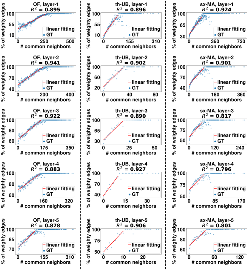
Figure 1: Fractions of strong edges grow nearly linearly until a saturation point. We also report the $R^{2}$ of linear fitting before the saturation point. The $R^{2}$ is high in each layer, indicating that the growth is consistently nearly linear. See the supplementary material (Bu et al., 2022) for the full results.

5.2 Observation 1: the fractions of weighty edges

We have shown that the numbers of CNs and the repetition (i.e., weightiness in layer-$1$) of edges are highly correlated. We examine this phenomenon in more layers and study the detailed numerical relations between the number $c$ of CNs and the corresponding fraction of weighty edges (FoWE) $f_{c;i}$. In Figure 1, for each dataset and each layer-$i$ with $1\leq i\leq 5$, we plot the FoWEs, where we can observe that the FoWEs grow nearly linearly with the number of CNs until some saturation point (see Definition 3) such that the FoWEs after the saturation point are almost $100\%$. In Figure 1, we also show the results of the linear fitting for the points truncated before the corresponding saturation point with the $R^{2}$ values, where we can see consistently strong linear correlations. We formally define the saturation point of the fractions of weighty edges (FoWEs) as the minimum number $c^{*}$ such that all the edges in $E_{c^{*};i}$ are weighty edges.

Definition 3 (Saturation points of the fraction of weighty edges).

Given $G$ and $i$, the saturation point $c_{i}^{*}(G)$ of the fractions of weighty edges is defined as $\min\{c\in\mathbb{N}:f_{c;i}=1\}$.

Remark 1.

Theoretically, the above definition of saturation point may appear less robust since a single edge that is not weighty can affect the whole group of edges sharing the same number of CNs. We use such a definition for simplicity and clarity. In Appendix C, we discuss this issue and show the practical reasonableness of this definition on the datasets used in our empirical evaluation.

Observation 1 (Nearly linear growth of FoWEs).

On each dataset, in each layer, the FoWEs grow nearly linearly with the number of CNs and become almost all $100\%$ after some saturation point.

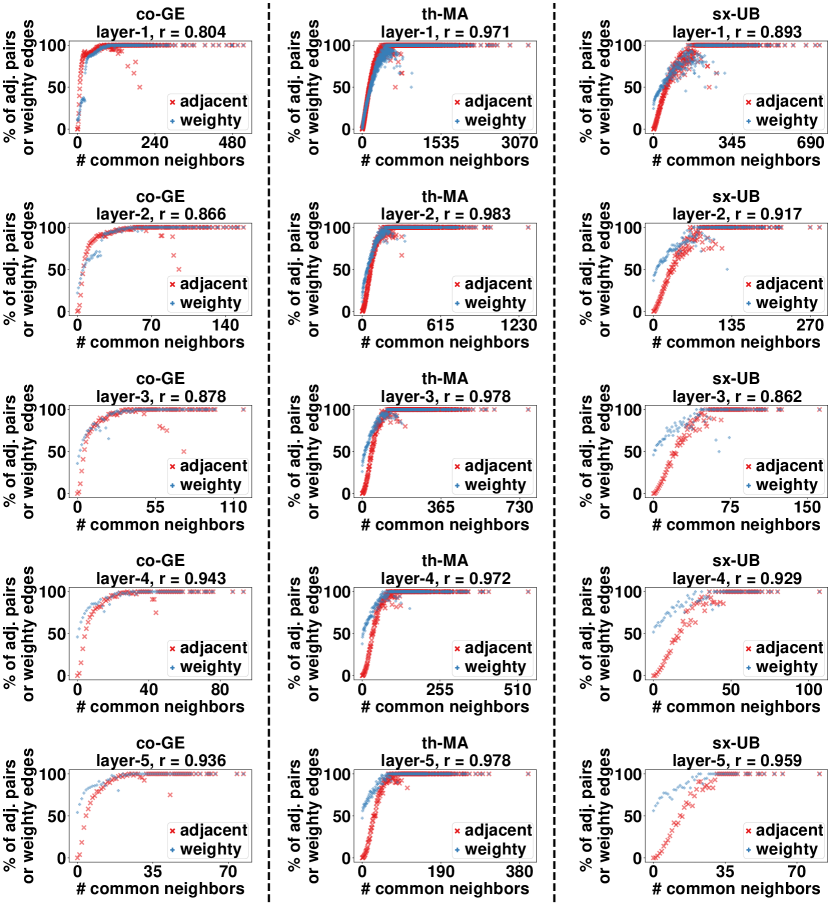
Figure 2: The fractions of (a) adjacent pairs and (b) weighty edges within each group with the same number of common neighbors are similar. We report Pearson’s $r$ between the two fractions, which is high in each layer. Note that for each dataset, the range of the $x$-axis changes over layers, which is because the maximum number of common neighbors changes over layers. Also, we do not compare the fractions across different layers but only compare them within each layer. The full results are in the supplementary material (Bu et al., 2022).

5.3 Observation 2: adjacency and weightiness

The number of CNs has been widely used for link prediction (Liu et al., 2011; Güneş et al., 2016), i.e., inferring the adjacency between node pairs. In the above Observation 1, we have shown the connection between the number of CNs and the weightiness of edges. Are the adjacency of pairs and the weightiness of edges also quantitatively related? In Figure 2, for each dataset and each layer-$i$ with $1\leq i\leq 5$, we report how (a) the fraction of adjacent pairs within each group of pairs (i.e., $\tilde{f}_{c;i}$) and (b) the fraction of weighty edges within each group of edges (i.e., $f_{c;i}$) depend on the number of CNs, where consistently high Pearson correlation coefficients are observed. We summarize our observation w.r.t this similarity as follows.

As we have mentioned, the information of CNs has been used for link prediction  (Wang et al., 2015) and for indicating the significance of individual edges (Ahmad et al., 2020; Cao et al., 2015; Zhu and Xia, 2016), where the assumption is usually qualitative, e.g., node pairs between two nodes sharing more CNs are more likely to be adjacent (or more important). However, no existing works study the quantitative relation between the adjacency of pairs and the weightiness (repetition) of edges w.r.t the number of CNs in a unified way and compare them with each other.

Table 4: The saturation point of the fractions of weighty edges and that of the fractions of adjacent pairs are consistently close. For each layer of each dataset, we report the saturation point of the fractions of adjacent pairs on the left and that of the fractions of weighty edges on the right.

dataset	layer-$1$	layer-$2$	layer-$3$	layer-$4$	layer-$5$
OF	241/271	190/192	157/156	134/137	119/101
FL	64/66	31/31	17/17	-	-
th-UB	73/87	30/31	19/20	18/11	15/11
th-MA	372/401	145/153	114/114	84/67	63/59
th-SO	685/750	208/205	134/129	97/82	74/72
sx-UB	152/149	63/69	48/42	36/27	31/22
sx-MA	185/181	113/102	75/63	60/49	51/41
sx-SO	886/749	407/324	221/203	169/130	120/103
sx-SU	202/206	96/93	63/54	48/37	36/27
co-DB	83/88	36/29	22/24	20/21	16/16
co-GE	74/92	52/49	34/40	28/30	24/21

Similar to the saturation point of FoWEs, we also defined the saturation point of the fractions of adjacent pairs (FoAPs) as the minimum number $c^{*}$ such that all the pairs in $R_{c^{*};i}$ are adjacent pairs.

Definition 4 (Saturation points of the fractions of adjacent pairs).

Given $G$ and $i$, recall that the saturation point $c_{i}^{*}(G)$ of the fractions of weighty edges is defined as $\min\{c\in\mathbb{N}:f_{c;i}=1\}$, the saturation point $\tilde{c}_{i}^{*}(G)$ of the fractions of adjacent pairs is defined as $\min\{c\in\mathbb{N}:R_{c;i}=E_{c;i}\}$.

As shown in Table 4, we observe that the saturation point of the FoWEs is consistently similar to that of the FoAPs (see Figure 2).

Observation 2 (Similarity between pair-adjacency and edge-weightiness).

On each dataset, in each layer, the trends of the fractions of adjacent pairs and the fractions of weighty edges w.r.t the number of CNs have a high correlation (see the consistently high Pearson’s $r$ values), and the saturation point of the FoWEs is close to that of the FoAPs.

5.4 Observation 3: a power law across layers

The previous observations describe some patterns within each layer. Is there any pattern that connects different layers? For each layer-$i$, we collect the information of $f_{0;i}$ (FoWE of the group of edges without CNs in layer-$i$) and $f_{overall;i}$ (the overall FoWE of all the edges in layer-$i$). By doing so, we obtain two sequences ($f_{0;i}$’s and $f_{overall;i}$’s) across different layers. We observe a consistent and strong power law between the two sequences, which we visualize in Figure 3. In the figure, for each dataset, we plot (a) the point $(f_{overall;i},f_{0;i})$ for each $1\leq i\leq 10$ in the log-log scale and (b) the power-law fitting line, which is linear in the log-log scale. The consistent and strong power law is clearly observed.

Observation 3 (A power law across layers).

On each dataset, across the layers, the FoWEs of the group of edges sharing no CNs and the overall FoWEs of all edges follow a strong power law.

Remark 2.

All the above observations are based on layer structures. For weighted graphs with positive-integer edge weights, decomposing such graphs into layers is straightforward, while for weighted graphs with real-valued edge weights, we can convert the edge weights into integers by rounding or other ways. Moreover, in the datasets used in this work, the edge weights represent the number of occurrences. Therefore, the observations may not hold on weighted graphs where the edge weights have other real-world meanings. See Appendix A for more discussions.

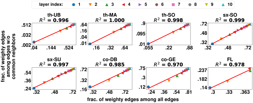
Figure 3: Consistent and strong power laws exists between the fractions of weighty edges of (a) those without common neighbors and (b) those of all edges. We also report the $R^{2}$ of power-law fitting. The $R^{2}$ is consistently close to $1$ for all datasets, indicating consistently strong power laws. See the supplementary material (Bu et al., 2022) for the full results.

6 Proposed algorithm: PEAR

In this section, we propose PEAR (Pattern-based Edge-weight Assignment on gRaphs), an algorithm with only two parameters that assigns weights to a given topology. PEAR produces the edge weights layer by layer based on the above observations. Below, we shall describe the mathematical formulation of our observations and then the detailed procedure of PEAR.

6.1 Formulation of the observations

In Section 5, we describe the patterns that we have observed on the real-world datasets. For constructing an algorithm, we shall first mathematically formulate the observations. In the formulation, we may idealize the observations into simple, intuitive, and deterministic formulae.

Linear growth of FoWEs.whiteLinear growth of FoWEs. In Observation 1, we have mentioned that the fractions of weighty edges (FoWEs) grow nearly linearly with the number of CNs with some saturation points consistently over all datasets and all layers. In our algorithm PEAR, we assume perfect linearity, and we formulate this phenomenon as follows:

$$f_{c;i}(G)=\min(1,f_{0;i}(G)+(1-f_{0;i}(G))\frac{c}{c_{i}^{*}(G)}),\forall G,i,c,$$ (1)

where $c_{i}^{*}(G)$ is the saturation point of FoWEs in $G_{i}$. By this formulation, $f_{c;i}=f_{0;i}$ when $c=0$, and it increases with the number of CNs in a ratio of $(1-f_{0;i})/c_{i}^{*}$ until $f_{c;i}=1$ when $c$ reaches $c_{i}^{*}$ and stays with $f_{c;i}=1$ thereafter.

Algorithm 1 PEAR for edge-weight assignment

Input: (1) $\mkern 1.5mu\overline{\mkern-1.5muG\mkern-1.5mu}\mkern 1.5mu=(V,E)$, (2) power-law parameters $a$ and $k$
      Output: weight assignment $W$

1:$G_{1}\leftarrow\mkern 1.5mu\overline{\mkern-1.5muG\mkern-1.5mu}\mkern 1.5mu$

2:$W_{e}\leftarrow 1,\forall e\in E$

3:for $i=1,2,3,\ldots$ do

4:     if $\tilde{c}_{i}^{*}$ does not exist or $\sum_{c<\tilde{c}_{i}^{*}}|E_{c;i}|=0$ then

5:         Break

6:     end if

7:     $|E_{i+1}|\leftarrow$ the solution in $(0,|E_{i}|)$ of Equation (8) (Property (3))

8:     $f_{0;i}\leftarrow a(|E_{i+1}|/|E_{i}|)^{k}$ (Eq. (4))

9:     $c_{i}^{*}\leftarrow\tilde{c}_{i}^{*}$ (Property (2))

10:     $C_{i}\leftarrow\{|CN_{e}|:e\in E_{i}\}$

11:     $E_{c}\leftarrow\{e\in E_{i}:|CN_{e}|=c\},\forall c\in C_{i}$

12:     $f_{c;i}\leftarrow\min(1,f_{0;i}+(1-f_{0;i}){c}/{c_{i}^{*}}),\forall c\in C_{i}$ (Property (1))

13:     $E_{i+1}\leftarrow\emptyset$

14:     for each $c\in C_{i}$ do

15:         $\hat{E}_{c}\leftarrow$ sample $f_{c;i}|E_{c}|$ (rounded) edges in $E_{c}$ uniformly at random

16:         $E_{i+1}\leftarrow E_{i+1}\cup\hat{E}_{c}$

17:     end for

18:     $W_{e}\leftarrow i+1,\forall e\in E_{i+1}$

19:     $G_{i+1}\leftarrow(\bigcup_{e\in E_{i+1}}e,E_{i+1})$

20:end for

21:return $W$

Saturation points.whiteSaturation points. In Observations 2 and 1, we have mentioned the similarity between the trends of the fraction of adjacent pairs and the FoWEs and we have further pointed out that the saturation points of the two kinds of fractions are close. In the algorithm, we assume equality between $\tilde{c}_{i}^{*}$ and $c_{i}^{*}$, and we formulate it as follows:

$$c_{i}^{*}(G)=\tilde{c}_{i}^{*}(G),\forall G,i,$$ (2)

where recall that $\tilde{c}_{i}^{*}(G)=\min\{c:R_{c;i}(G)=E_{c;i}(G)\}$ and $R_{c;i}(G)$ is the set of node pairs sharing $c$ CNs in $G_{i}$.

The power law across layers.whiteThe power law across layers. In Observation 3, we have mentioned that the FoWEs of the group of edges sharing no CNs and the overall FoWEs of all edges follow a strong power law. In the algorithm, assuming a perfect power law, we formulate it as follows:

$$f_{0;i}(G)=a(G)f_{overall;i}^{k(G)},\forall G,i,$$ (3)

where $a(G)$ and $k(G)$ are the two parameters of the power law which may vary for each different graph $G$.

With Properties (1)-(3) formulated and explicitly described, we are now ready to re-state Problem 1 in a more formal and specific way.

Problem 2 (Formal).

Given an unweighted graph $\mkern 1.5mu\overline{\mkern-1.5muG\mkern-1.5mu}\mkern 1.5mu=(V,E)$, we aim to generate edge weights $W:E\rightarrow\mathbb{N}$ that satisfy Properties (1)-(3).

6.2 Algorithmic details

Now we are ready to describe the algorithmic details of PEAR (Algorithm 1), which combines all the above formulae to produce the edge weights layer by layer. From now on, we suppose that $G$ is given as an input and thus fixed. By Equation (3) and the definition of $f_{overall;i}=|E_{i+1}/E_{i}|$, we have

$$f_{0;i}=a(|E_{i+1}|/|E_{i}|)^{k},\forall i.$$ (4)

For each layer-$i$, the total number $|E_{i+1}|$ of weighty edges should be equal to the summation of the numbers of weighty edges in all the $E_{c;i}$’s. By Equations (1) and (2), it gives

$$|E_{i+1}|= \sum_{c}|E_{c;i}|f_{c;i}=\sum_{c}|E_{c;i}|\min(1,f_{0;i}+(1-f_{0;i}){c}/{c_{i}^{*}})$$

$$= \sum_{c}|E_{c;i}|\min(1,f_{0;i}+(1-f_{0;i}){c}/{\tilde{c}_{i}^{*}}).$$ (5)

Note that $\tilde{c}_{i}^{*}$ can be obtained from the given topology when $i=1$ or from the currently generated layers when $i>1$ (Line 9). We expand Equation (6.2) to get

$$|E_{i+1}|= \sum_{c\leq\tilde{c}_{i}^{*}}|E_{c;i}|(f_{0;i}+(1-f_{0;i}){c}/{\tilde{c}_{i}^{*}})+\sum_{c>\tilde{c}_{i}^{*}}|E_{c;i}|$$

$$= f_{0;i}\sum_{c\leq\tilde{c}_{i}^{*}}|E_{c;i}|(\tilde{c}_{i}^{*}-c)/{\tilde{c}_{i}^{*}}+\sum_{c}|E_{c;i}|\min(1,{c}/{\tilde{c}_{i}^{*}}),$$ (6)

which further gives the relation between $f_{0;i}$ and $\tilde{c}_{i}^{*}$:

$$f_{0;i}=\frac{|E_{i+1}|-\sum_{c}|E_{c;i}|\min(1,{c}/{\tilde{c}_{i}^{*}})}{\sum_{c\leq\tilde{c}_{i}^{*}}|E_{c;i}|(\tilde{c}_{i}^{*}-c)/{\tilde{c}_{i}^{*}}}.$$ (7)

Equations (4) and (7) give us two different expressions of $f_{0;i}$ and we can use them to obtain $|E_{i+1}|$ by solving the following equation:

$$a(|E_{i+1}|/|E_{i}|)^{k}=\frac{|E_{i+1}|-\sum_{c}|E_{c;i}|\min(1,{c}/{\tilde{c}_{i}^{*}})}{\sum_{c<\tilde{c}_{i}^{*}}|E_{c;i}|(\tilde{c}_{i}^{*}-c){\tilde{c}_{i}^{*}}}.$$ (8)

Remark 3.

In Equation (8), the denominator is zero only when $E_{c;i}=\emptyset$ for each $c\leq\tilde{c}_{i}^{*}$, which implies that all the edges are strong edges and the generated edge weights are not meaningful.

Theorem 1.

Assume that $\tilde{c}_{i}^{*}>0$ exists and $\sum_{c<\tilde{c}_{i}^{*}}|E_{c;i}|>0$. If $a<1$ and $k>1$, then in the range $(0,|E_{i}|)$, Equation (8) has a unique solution $|E_{i+1}|\in(0,|E_{i}|)$.

Proof.

Define

$$g(x)=a(\frac{x}{|E_{i}|})^{k}-\frac{x-\sum_{c}|E_{c;i}|\min(1,{c}/{\tilde{c}_{i}^{*}})}{\sum_{c\leq\tilde{c}_{i}^{*}}|E_{c;i}|(\tilde{c}_{i}^{*}-c){\tilde{c}_{i}^{*}}}$$

on $x\in[0,|E_{i}|]$. We have

$$g(0)=\frac{\sum_{c}|E_{c;i}|\min(1,{c}/{\tilde{c}_{i}^{*}})}{\sum_{c\leq\tilde{c}_{i}^{*}}|E_{c;i}|(\tilde{c}_{i}^{*}-c){\tilde{c}_{i}^{*}}}>0$$

and $g(|E_{i}|)=a-1<0$. Since $f$ is continuous, by the intermediate value theorem (see also Bolzano’s theorem), we have at least one solution in the range $(0,|E_{i}|)$. For the uniqueness, we have

$$f^{\prime\prime}(x)=ak(k-1)x^{k-2}/|E_{i}|^{k}>0,\forall x\in(0,|E_{i}|)$$

(i.e., $f$ is convex on $(0,|E_{i}|)$). Assume that we have two roots $0<x_{1}<x_{2}<|E_{i}|$, let $t=(|E_{i}|-x_{2})/(|E_{i}|-x_{1})\in(0,1)$, then by the convexity of $f$ we have

$$0=g(x_{2})=g(tx_{1}+(1-t)|E_{i}|)\leq tg(x_{1})+(1-t)g(|E_{i}|)=(1-t)g(|E_{i}|)<0,$$

completing the proof by contradiction. ∎

After obtaining $|E_{i+1}|$ (Line 7), we use Equation (4) to compute $f_{0;i}$ (Line 8), and then use Equation (1) with $c_{i}^{*}=\tilde{c}_{i}^{*}$ to compute all $f_{c;i}$’s (Lines 9 and 12). Then for each $c$, we sample $f_{c;i}|E_{c}|$ edges uniformly at random in $E_{c}$ in the current layer $G_{i}$ to be weighty edges, assign the edge weights accordingly, and construct the next layer $G_{i+1}$ (Lines 13-19). We repeat the process layer after layer. By Theorem 1, if we have a valid saturation point $\tilde{c}_{i}^{*}$ and there exist edges sharing less than $\tilde{c}_{i}^{*}$ CNs, we can always obtain a unique solution of $|E_{i+1}|$ from Equation (8), and thus the whole process can continue. If any of the conditions are not met, the process terminates, and the current edge weights are returned as the final output (Lines 4 and 21).

The following theorem shows the time complexity of Algorithm 1.

Theorem 2.

Given an input graph $\mkern 1.5mu\overline{\mkern-1.5muG\mkern-1.5mu}\mkern 1.5mu=(V,E)$ and two parameters $a$ and $k$, Algorithm 1 takes $O(i_{max}\sum_{v\in V}d_{v}^{2}))$ time to output a weight assignment $W$, where $i_{max}$ is the maximum layer index such that $G_{i_{max}}$ is non-empty, i.e., the maximum weight in the output.

Proof.

We shall show that it takes $O(\sum_{v\in V}d_{v}^{2})$ to generate each layer. The time complexity consists of (1) that of computing $\tilde{c}_{i}^{*}$ (Line 9) and (2) that of sampling weighty edges (Lines 14-17). For (1), checking the CNs of all pairs can be done by enumerating all neighbor pairs of each node, which takes $O(\sum_{v\in V}d_{v}^{2}(G_{i}))=O(\sum_{v\in V}d_{v}^{2}(G))$ time. For (2), sampling among $E_{i}$ takes $O(|E_{i}|)=O(|E|)=O(\sum_{v\in V}d_{v}(G))$ time, completing the proof. ∎

The following theorem states that Algorithm 1 indeed preserves all the formulated properties and is What are the relations between the edge weights and the topology in real-world graphs? Given only the topology of a graph, how can we assign realistic weights to its edges based on the relations? Several trials have been done for edge-weight prediction where some unknown edge weights are predicted with most edge weights known. There are also existing works on generating both topology and edge weights of weighted graphs. Differently, we are interested in generating edge weights that are realistic in a macroscopic scope, merely from the topology, which is unexplored and challenging. To this end, we explore and exploit the patterns involving edge weights and topology in real-world graphs. Specifically, we divide each graph into layers where each layer consists of the edges with weights at least a threshold. We observe consistent and surprising patterns appearing in multiple layers: the similarity between being adjacent and having high weights, and the nearly-linear growth of the fraction of edges having high weights with the number of common neighbors. We also observe a power-law pattern that connects the layers. Based on the observations, we propose PEAR, an algorithm assigning realistic edge weights to a given topology. The algorithm relies on only two parameters, preserves all the observed patterns, and produces more realistic weights than the baseline methods with the same number of, or even more, parameters. a valid approach for Problem 2.

Theorem 3.

Given any $\bar{G}=(V,E)$, $a$, and $k$, the output of PEAR (Algorithm 1) satisfies Properties (1)-(3) up to integer rounding.

Proof.

Property (1) is explicitly preserved by Line 12, and Property (2) is explicitly preserved by Line 9. Regarding Property (3), since Property (1) is preserved, the solution of Equation (8) which combines Properties (1) and (3) preserves Property (3), completing the proof. ∎

Remark 4.

Due to the interconnectedness of all the three properties, for any fixed $a$ and $k$, the output of PEAR is unique up to the sampling (Line 14-17), which is evidentially supported by the small standard variations in Tables 5 and 6.

7 Experiments

In this section, through experiments on the real-world graphs, we shall show that, in most cases, PEAR generates realistic edge weights for a given topology with only two parameters and without sophisticated searching or fine-tuning on the parameters.

7.1 Baseline methods and experimental settings

The following baseline methods (PRD, SCN, SEB, PEB, and STC) are unsupervised in that they do not use any explicit ground truth edge-weight information. However, for these methods to output meaningful predictions, we provide the ground-truth number of edges for each layer-$i$ (i.e., $|E_{i}|$) with $2\leq i\leq 5$ to them. Such additional information is not provided to PEAR.

• PRD (purely random). The PRD method repeatedly uniformly at random chooses an edge and increments its weight until the $|E_{i}|$’s are satisfied.

• SCN (sorting-CN). Instead of random sampling, the SCN method sorts the edges by the number of CNs and assigns the weights accordingly (higher weights to the edges with more CNs).

• SEB (sorting-embedding). The SEB method sorts the edges by the inner product of the node embeddings of the two endpoints of each edge and assigns higher weights to the edges with higher inner products. The node embeddings are produced by two different methods, RandNE (Zhang et al., 2018; Rozemberczki et al., 2020) and node2vec (Grover and Leskovec, 2016). We use SEB-R and SEB-N to denote the results using RandNE and node2vec, respectively. The feature dimension is set as $32$, and all the other parameters are kept the same as in the original paper.

• PEB (probability-embedding). The PEB method uses node embeddings as in SEB, and it repeatedly chooses an edge and increments its weight until the $|E_{i}|$’s are satisfied, where the exponential of the inner product of the node embeddings of the two endpoints of each edge is used as the weight of the edge in the sampling. We use PEB-R and PEB-N to denote the results using RandNE and node2vec, respectively.

• STC (strong triadic closure). The STC method makes use of the strong triadic closure (Sintos and Tsaparas, 2014) (STC) principle. Specifically, for each layer-$i$, the STC method first uses a greedy algorithm to maximize the number of candidate weighty edges in the layer without having any open triangle (i.e., three nodes $v_{1},v_{2},v_{3}$ s.t. the two edges $(v_{1},v_{2})$ and $(v_{1},v_{3})$ exist and $(v_{2},v_{3})$ does not exist). After that, the STC method uniformly at random samples $|E_{i}|$ weighty edges among all the candidates.

By contrast, for the proposed method PEAR, we only consider two settings $(a,k)\in\{(0.98,1.02),(0.7,1.3)\}$, where for the two co datasets and the four sx datasets we use $(a,k)=(0.98,1.02)$; and for the remaining datasets we use $(a,k)=(0.7,1.3)$. For each dataset, we report the results in the better setting. Note that these settings are chosen without relying on ground-truth weights. Specifically, when we choose the parameters, we simply move two parameters $a$ and $k$ in the opposite directions, while keeping $a+k=2$, so that all the candidate parameter settings satisfy the assumptions in Theorem 1. Also, the best-performing settings show clear domain-based patterns. Specifically, we can use the same parameter setting for datasets in the same domain. Although it is challenging to find the best-performing setting for a dataset merely based on its topology, the structural similarity between datasets within the same real-world domain (Chakrabarti and Faloutsos, 2006; Wills and Meyer, 2020) can be utilized to find a proper setting for each dataset based on the topology. See Appendix D for more discussions.

We also consider two supervised edge-weight prediction methods directly supervised by ground-truth edge weights. Notably, the supervised methods deal with the prediction task as a classification task and do not rely on the layer structure. We give the below supervised methods $10\%$ of the ground truth edge weights as the input training set (and another $10\%$ as the validation set if needed). We make sure each of the training set covers all five classes: edges of weight $1,2,3,4,\geq 5$, corresponding to the five layers we are studying. Notably, the supervised methods use much more parameters. The considered methods are:

• RFF (random forest-feature). The RFF method uses a random forest classifier (Breiman, 2001) with the 14 metrics we have used in Section 5.1 (see Table 3), which follows the procedure in a previous work (Fu et al., 2018) except for that the random forest is smaller and some metrics are not used due to its high computational cost as mentioned in Section 5.1. The hyperparameters of random forest are listed as follows: the number of trees = 32, the maximum depth of the tree = 5, and all the other parameters are kept the same as in the original work (Breiman, 2001).

• NEB (neural network-embedding). The NEB method uses a neural network consisting of one bilinear layer. For each edge, the node embeddings of both endpoints, which are obtained as in SEB, are used as the input, and the neural network is trained to minimize a classification loss (cross-entropy). We use NEB-R and NEB-N to denote the results using RandNE and node2vec, respectively.

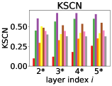
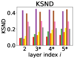
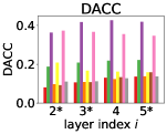
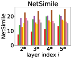
Figure 4: PEAR generates edge weights that are realistic in each layer. For each generated layer-$i$ with $i\in\{2,3,4,5\}$, each method, and each metric, we report the average over all datasets. We use asterisk marks ($*$) to indicate the 14 (out of 16) cases where PEAR performs best. See Tables 5 and 6 for the numerical comparison in detail.

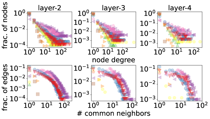
(a) threads-ubuntu, $(a,k)=(0.7,1.3)$

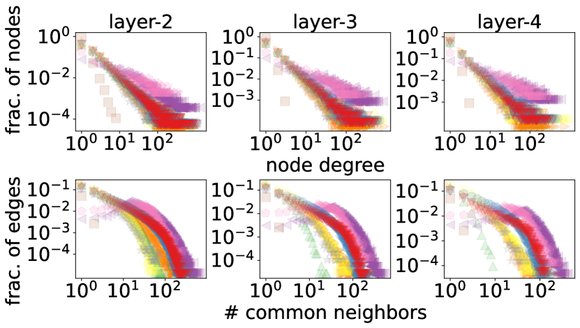
(b) sx-math, $(a,k)=(0.98,1.02)$

Figure 5: PEAR produces realistic edge weight. For each $i\in\{2,3,4\}$ and each method including the ground truth, we report the node-degree and number-of-CN distributions of the generated layer-$i$. See Tables 5 and 6 for the numerical comparison in detail.

Table 5: PEAR generates more realistic edge weights than the baseline methods in terms of KSCN and KSND. For each dataset and each metric, we report the average over the layers generated by each method, as well as the average (AVG) over all datasets and the average rank (A.R.), where the best result is in bold, and the second-best one is underlined (OOM = out of memory; FAIL = unable to output a meaningful layer). See the online appendix (Bu et al., 2022) for the full results.

metric method OF FL th-UB th-MA th-SO sx-UB sx-MA sx-SO sx-SU co-DB co-GE AVG A.R. KSCN PRD 0.542 0.522 0.722 0.840 0.768 0.242 0.486 0.259 0.299 0.656 0.731 0.55 8.36 SCN 0.485 0.661 0.528 0.579 0.634 0.782 0.681 0.795 0.768 0.661 0.573 0.65 8.18 SEB-R 0.217 0.401 0.712 0.773 0.737 0.252 0.362 0.305 0.328 0.484 0.488 0.46 7.00 SEB-N 0.475 0.184 0.670 0.601 0.624 0.100 0.221 0.159 0.237 0.155 0.199 0.33 3.73 PEB-R 0.626 0.368 0.665 0.711 0.607 0.109 0.310 0.137 0.154 0.529 0.577 0.44 4.82 PEB-N 0.626 0.368 0.665 0.711 0.607 0.109 0.310 0.137 0.154 0.529 0.577 0.44 4.82 STC 0.679 0.474 0.705 0.772 0.698 0.292 0.707 0.380 0.362 0.238 0.419 0.52 7.82 RFF 0.265 0.236 0.346 0.368 0.434 0.805 0.560 0.734 0.713 0.293 0.131 0.44 5.36 NEB-R 0.147 0.339 0.719 0.899 0.559 0.274 0.416 0.304 0.364 0.096 0.085 0.38 5.45 NEB-N 0.140 FAIL FAIL 0.901 0.732 0.304 0.749 0.137 0.277 0.224 0.383 FAIL 7.09 PEAR (ours) 0.074 0.241 0.168 0.186 0.126 0.076 0.072 0.239 0.103 0.329 0.181 0.16 2.18 ($\pm$0.003) ($\pm$0.017) ($\pm$0.015) ($\pm$0.006) ($\pm$0.008) ($\pm$0.003) ($\pm$0.001) ($\pm$0.001) ($\pm$0.002) ($\pm$0.013) ($\pm$0.008) KSND PRD 0.096 0.164 0.336 0.219 0.161 0.040 0.059 0.027 0.045 0.237 0.292 0.15 4.36 SCN 0.359 0.424 0.406 0.587 0.443 0.544 0.556 0.371 0.506 0.311 0.283 0.44 9.91 SEB-R 0.087 0.180 0.361 0.201 0.157 0.038 0.067 0.038 0.057 0.231 0.289 0.16 4.64 SEB-N 0.096 0.121 0.336 0.212 0.155 0.027 0.065 0.034 0.041 0.155 0.198 0.13 3.09 PEB-R 0.232 0.172 0.289 0.248 0.133 0.041 0.085 0.071 0.057 0.274 0.293 0.17 5.27 PEB-N 0.232 0.172 0.289 0.248 0.133 0.042 0.085 0.071 0.057 0.274 0.294 0.17 5.45 STC 0.577 0.385 0.452 0.441 0.397 0.303 0.492 0.531 0.354 0.306 0.374 0.42 10.00 RFF 0.115 0.146 0.267 0.388 0.322 0.602 0.416 0.246 0.410 0.217 0.121 0.30 6.64 NEB-R 0.148 0.108 0.389 0.430 0.326 0.128 0.163 0.346 0.194 0.055 0.113 0.22 6.18 NEB-N 0.085 FAIL FAIL 0.327 0.352 0.229 0.247 0.208 0.165 0.090 0.284 FAIL 7.09 PEAR (ours) 0.069 0.070 0.157 0.175 0.129 0.027 0.146 0.178 0.022 0.105 0.105 0.11 2.09 ($\pm$0.002) ($\pm$0.002) ($\pm$0.009) ($\pm$0.009) ($\pm$0.002) ($\pm$0.000) ($\pm$0.001) ($\pm$0.003) ($\pm$0.000) ($\pm$0.007) ($\pm$0.001)

Table 6: PEAR generates more realistic edge weights than the baseline methods in terms of DACC and NetSimile. For each dataset and each metric, we report the average over the layers generated by each method, as well as the average (AVG) over all datasets and the average rank (A.R.), where the best result is in bold, and the second-best one is underlined (OOM = out of memory; FAIL = unable to output a meaningful layer). See the online appendix (Bu et al., 2022) for the full results.

metric method OF FL th-UB th-MA th-SO sx-UB sx-MA sx-SO sx-SU co-DB co-GE AVG A.R. DACC PRD 0.291 0.184 0.239 0.371 0.211 0.036 0.139 0.036 0.047 0.370 0.376 0.21 8.45 SCN 0.166 0.417 0.434 0.457 0.486 0.587 0.523 0.520 0.589 0.160 0.129 0.41 9.00 SEB-R 0.060 0.135 0.235 0.356 0.204 0.035 0.118 0.036 0.048 0.271 0.213 0.16 6.55 SEB-N 0.246 0.036 0.215 0.311 0.190 0.018 0.102 0.026 0.039 0.054 0.046 0.12 3.55 PEB-R 0.240 0.131 0.225 0.313 0.190 0.023 0.064 0.024 0.018 0.344 0.341 0.17 4.64 PEB-N 0.240 0.131 0.225 0.313 0.190 0.023 0.063 0.024 0.017 0.344 0.341 0.17 4.45 STC 0.027 0.077 0.231 0.273 0.155 0.036 0.148 0.036 0.046 0.117 0.205 0.12 4.55 RFF 0.187 0.106 0.279 0.418 0.399 0.645 0.468 0.548 0.595 0.197 0.120 0.36 8.36 NEB-R 0.126 0.142 0.237 0.377 0.162 0.032 0.103 0.024 0.049 0.051 0.037 0.12 4.73 NEB-N 0.028 FAIL FAIL 0.378 0.195 0.042 0.173 0.030 0.031 0.087 0.175 FAIL 6.91 PEAR (ours) 0.158 0.080 0.129 0.262 0.146 0.016 0.043 0.037 0.023 0.227 0.127 0.11 3.27 ($\pm$0.006) ($\pm$0.007) ($\pm$0.004) ($\pm$0.001) ($\pm$0.001) ($\pm$0.000) ($\pm$0.000) ($\pm$0.000) ($\pm$0.001) ($\pm$0.005) ($\pm$0.004) NetSimile PRD 11.99 16.81 24.71 23.80 22.38 15.33 12.49 OOM 15.39 19.83 19.93 18.27 7.10 SCN 15.47 20.56 18.68 21.76 23.39 24.89 22.77 OOM 25.45 12.62 13.32 19.89 7.30 SEB-R 9.34 16.26 25.15 23.70 21.32 16.46 12.06 OOM 17.38 17.74 17.64 17.71 6.20 SEB-N 10.67 12.29 24.52 23.29 22.77 8.51 8.91 OOM 12.85 16.06 17.34 15.72 4.30 PEB-R 12.03 14.11 19.28 19.40 17.45 13.04 12.81 OOM 13.65 18.51 17.55 15.78 4.90 PEB-N 12.02 14.12 19.29 19.40 17.45 13.05 12.80 OOM 13.65 18.49 17.55 15.78 5.00 STC 23.57 21.16 27.70 26.03 23.08 24.04 25.53 OOM 25.08 21.35 22.27 23.98 10.00 RFF 12.26 13.81 16.51 18.10 18.96 25.61 20.87 OOM 25.42 14.71 7.54 17.38 5.30 NEB-R 11.10 12.95 21.31 22.88 20.49 17.11 14.20 OOM 19.27 9.73 8.89 15.79 4.90 NEB-N 6.21 FAIL FAIL 26.69 22.96 29.80 27.12 OOM 22.49 19.52 21.79 FAIL 9.20 PEAR (ours) 8.09 8.92 9.33 14.85 13.79 6.03 9.40 OOM 6.37 15.73 10.87 10.34 1.70 ($\pm$0.32) ($\pm$0.17) ($\pm$0.22) ($\pm$0.07) ($\pm$0.10) ($\pm$0.12) ($\pm$0.04) ($\pm$0.14) ($\pm$0.24) ($\pm$0.04)

7.2 Evaluation methods

We would re-emphasize that we aim to generate edge weights that are realistic in a macroscopic scope, and thus the evaluation should also be in a macroscopic scope. We report the following metrics including several graph statistics that have been widely used for evaluating graph generators (Leskovec et al., 2005; Shuai et al., 2013; Cao et al., 2015; Heath and Parikh, 2011) to compare, for each $2\leq i\leq 5$, the layer-$i$ produced by each method and the original one: (1) KS statistic for number-of-CN distributions (KSCN), (2) KS statistic for node-degree distributions (KSND), (3) difference in average clustering coefficients (DACC), and (4) a graph distance measure computed by NetSimile (Berlingerio et al., 2012). The intuition is that if two weighted graphs have similar layers with the same layer index, then the two weighted graphs are similar too. Note that the evaluation focuses on the first four layers since, for $i>5$, the ground-truth layer-$i$ is too small or too sparse in some datasets. See Appendix F for more analysis using graph motifs.

7.3 Results

First, we show how the methods perform on each dataset. In Tables 5 and 6, for each dataset, each metric, and each method, we report the average value over all the generated layers. For PEAR, the mean value and the standard deviation over three trials of each setting are reported. Overall, PEAR has the best average value and the highest average rank among all the methods w.r.t each metric. Specifically, PEAR achieves an average rank of $2.18$, $2.09$, $3.27$, and $1.70$ (there are $11$ methods in total), w.r.t the metric KSCN, KSNC, DACC, and NetSimile, respectively. Notably, although supervised with some ground-truth edge weights, the supervised baseline methods do not show clear superiority over the unsupervised ones. In our understanding, this is because the edge-weight classes (i.e., layers) are highly imbalanced (i.e., the numbers of edges with different weights vary a lot), while the ground-truth numbers of edges in each edge-weight class are provided to the unsupervised baseline methods including SEB are helpful. Also, the methods using sophisticated embeddings are sometimes even worse than SCN which assigns edge weights using a simple heuristic based on the number of CNs. In our understanding, this is because local information is important (according to our observations), while the embedding-based methods focus on higher-order information which can be confusing and harmful to the prediction results.

In Figure 5, for the two datasets th-UB and sx-MA, and for $i\in\{2,3,4\}$, we report the node-degree and edge-CN distributions of the layer-$i$ generated by each method, where the layers generated by PEAR have the two distributions closest to the original ones. For each baseline method using embeddings, between the two variants using RandNE and node2vec, we report the results of the variant that performs better.

We also study how the performance varies across generated layers. In Figure 4, for each method, each metric, and each layer index $i$, we report the average over all datasets. Again, for each baseline method using embeddings, between the two variants using RandNE and node2vec, we report the results of the variant that performs better. Overall, PEAR performs best for each layer.

8 Conclusion and future directions

In this work, we explored the relations between edge weights and topology in real-world graphs. We proposed a new concept called layers (Definition 1) with several related concepts (Definition 2), and observed several pervasive patterns (Observations 2-3). We also proposed PEAR (Algorithm 1), a weight-assignment algorithm with only two parameters, based on the formulation of our observations (Properties (1)-(3) and Equations (4)-(8)). In our experiments on eleven real-world graphs, we showed that PEAR generates more realistic edge weights than the baseline methods, including those requiring much more prior knowledge and parameters (Tables 5-6 and Figures 5-4).

The observations in this work are macroscopic and the proposed model is based on those observations. Although macroscopic patterns are relatively more robust to outliers compared to microscopic ones, it is still possible that outliers can impair the performance of our method. We plan to explore and examine how outliers can affect the performance of our method and the corresponding solutions. We studied weighted graphs with positive-integer edge weights, and we plan to extend the study on the interplay between edge weights and topology to real-valued edge weights. We studied the average behavior of each group of edges or pairs with the same number of common neighbors, and we plan to further explore the patterns within each group. We also plan to study how the two parameters of PEAR affect the output.

Table 7: The numbers of common neighbors are simple yet indicative. Additional results: we report the area under the ROC curve (AUC) of the logistic regression fit to the sequences of each quantity and the binary indicators of repetition.

dataset	NC	SA	JC	HP	HD	SI	LI	AA	RA	PA	FM	DL	EC	LP
OF	0.704	0.636	0.641	0.508	0.637	0.641	0.632	0.707	0.723	0.705	0.571	0.692	0.666	0.704
FL	0.676	0.664	0.657	0.619	0.647	0.657	0.479	0.698	0.725	0.629	0.546	0.606	0.610	0.674
th-UB	0.890	0.689	0.702	0.590	0.704	0.702	0.499	0.879	0.832	0.122	0.805	0.781	0.872	0.895
th-MA	0.843	0.751	0.701	0.587	0.689	0.701	0.662	0.845	0.823	0.834	0.800	0.741	0.801	0.844
th-SO	0.831	0.717	0.687	0.646	0.676	0.687	0.580	0.837	0.808	0.199	0.796	0.756	0.768	0.827
sx-UB	0.586	0.579	0.576	0.565	0.575	0.576	0.446	0.585	0.581	0.592	0.582	0.576	0.577	0.598
sx-MA	0.635	0.631	0.613	0.574	0.606	0.613	0.506	0.639	0.645	0.623	0.605	0.595	0.611	0.634
sx-SO	0.562	0.561	0.551	0.560	0.549	0.551	0.463	0.563	0.566	0.553	0.555	0.552	0.538	0.563
sx-SU	0.588	0.576	0.570	0.570	0.569	0.570	0.455	0.587	0.583	0.593	0.585	0.580	0.578	0.596
co-DB	0.624	0.529	0.523	0.530	0.521	0.523	0.587	0.617	0.586	0.360	0.624	0.627	0.601	0.630
co-GE	0.684	0.527	0.512	0.551	0.505	0.512	0.616	0.687	0.633	0.679	0.654	0.658	0.651	0.686
avg.	0.693	0.624	0.612	0.573	0.607	0.612	0.539	0.695	0.682	0.535	0.648	0.651	0.661	0.696
avg. rank	3.00	8.18	9.18	11.18	11.18	9.18	12.45	2.45	4.18	7.27	7.36	7.73	7.73	2.27

Appendix A General edge weights

As mentioned in Remark 2, all the observations in this work are based on layer structures, and the edge weights are limited to integer ones representing the number of occurrences. In order to examine the generality of our observations and the proposed algorithm, we examined several blockchain transaction datasets (Kılıç et al., 2022a, b), where each edge weight is a real number representing the amount of the corresponding transaction. On the transaction datasets mentioned above, the correlations between the edge weights and the number of common neighbors are very low (consistently less than $0.1$). Therefore, our observations and the proposed algorithm can not be directly applied to these datasets, which is a limitation of this work.

For general weighted graphs, we may make use of the known observation that real-world weighted graphs often have a heavy-tailed edge-weight distribution (Barrat et al., 2004; Kumar et al., 2020; Starnini et al., 2017). We leave as a potential future direction the exploration of the relation between edge weights and the number of common neighbors on weighted graphs with more general edge weights, as well as weighted graphs with edge weights having different real-world meanings (other than the number of occurrences).

Appendix B The indicativeness of the number of common neighbors

In Section 5.1, we have compared the indicativeness of the number of common neighbors with some baseline quantities measured by the point-biserial correlation coefficients (which are mathematically equivalent to the Pearson correlation coefficients). We would like to also examine this relation using other metrics, e.g., the area under the ROC curve (AUC).

In Table 7, we report the additional results measured by the AUC. Specifically, for each quantity, we first perform logistic regression between the sequence of the quantity and the binary indicators of repetition, then we compute the AUC of the output prediction. Although there are some baseline quantities achieving marginally higher AUC values, the number of common neighbors is still one of the most promising quantities, especially when we consider its simplicity.

Table 8: The saturation point of the fractions of adjacent pairs does not change much when we change the threshold in the definition from $100\%$ to $99\%$. For each layer of each dataset, we report the saturation point of the fractions of adjacent pairs with threshold $100\%$ on the left and the saturation point with threshold $99\%$ on the right.

dataset	layer-$1$	layer-$2$	layer-$3$	layer-$4$	layer-$5$
OF	241/234	190/190	157/157	134/134	119/119
FL	64/64	31/31	17/17	-	-
th-UB	73/73	30/30	19/19	18/18	15/15
th-MA	372/372	145/145	114/114	84/84	63/63
th-SO	685/685	208/208	134/134	97/97	74/74
sx-UB	152/152	63/63	48/48	36/36	31/31
sx-MA	185/185	113/113	75/75	60/60	51/51
sx-SO	886/886	407/407	221/221	169/169	120/120
sx-SU	202/202	96/96	63/63	48/48	36/36
co-DB	83/83	36/20	22/17	20/17	16/14
co-GE	74/74	52/46	34/32	28/27	24/22

Appendix C Saturation points

In Definition 4, we have defined the saturation point of the fraction of weighty edges (adjacent pairs) as the number $c$ of common neighbors such that all (i.e., $100\%$) the edges (pairs) sharing $c$ common neighbors are weighty (adjacent). Theoretically, this definition can be less robust since a single edge (pair) that is not weighty (adjacent) can affect the whole group of edges (pairs) sharing the same number of common neighbors. We have chosen to use the current definition for simplicity and clarity, while it is possible to make the concept more robust by using a less “absolute” threshold, e.g., “$99\%$”.

In Table 8, we show how the saturation points in the datasets used in our experiments change when we change the “$100\%$” in the definition to “$99\%$”. In the real-world datasets that we use, such a change makes no big difference. Therefore, we claim that such a simple and clear definition is expected to work well in practice, but practitioners may take the issue discussed above into consideration for better robustness.

Table 9: The parameter sensitivity results of PEAR. We report the performance of PEAR with four different parameter settings on the eleven real-world datasets used in our experiments, with the average rank of PEAR among all the baseline methods and PEAR for each parameter.

metric KSCN KSND DACC NetSimile dataset (0.98, 1.02) (0.7, 1.3) (0.98, 1.02) (0.7, 1.3) (0.98, 1.02) (0.7, 1.3) (0.98, 1.02) (0.7, 1.3) OF 0.391$\pm$0.002 0.074$\pm$0.003 0.254$\pm$0.000 0.069$\pm$0.002 0.057$\pm$0.001 0.158$\pm$0.006 12.754$\pm$0.038 8.087$\pm$0.320 FL 0.425$\pm$0.001 0.241$\pm$0.017 0.159$\pm$0.002 0.070$\pm$0.002 0.141$\pm$0.003 0.080$\pm$0.007 16.563$\pm$0.063 8.918$\pm$0.171 th-UB 0.482$\pm$0.002 0.168$\pm$0.015 0.188$\pm$0.002 0.157$\pm$0.009 0.187$\pm$0.001 0.129$\pm$0.004 18.661$\pm$0.031 9.327$\pm$0.224 th-MA 0.239$\pm$0.003 0.186$\pm$0.006 0.071$\pm$0.001 0.175$\pm$0.000 0.151$\pm$0.003 0.262$\pm$0.001 15.680$\pm$0.028 14.854$\pm$0.074 th-SO 0.544$\pm$0.001 0.126$\pm$0.008 0.109$\pm$0.002 0.129$\pm$0.002 0.189$\pm$0.000 0.146$\pm$0.001 18.698$\pm$0.069 13.786$\pm$0.098 sx-UB 0.076$\pm$0.003 0.416$\pm$0.003 0.027$\pm$0.000 0.118$\pm$0.010 0.016$\pm$0.000 0.071$\pm$0.004 6.026$\pm$0.115 17.414$\pm$0.094 sx-MA 0.072$\pm$0.001 0.176$\pm$0.009 0.146$\pm$0.001 0.098$\pm$0.003 0.043$\pm$0.000 0.059$\pm$0.000 9.397$\pm$0.041 11.684$\pm$0.084 sx-SO 0.239$\pm$0.001 0.315$\pm$0.004 0.178$\pm$0.003 0.202$\pm$0.001 0.037$\pm$0.000 0.038$\pm$0.001 N/A N/A sx-SU 0.103$\pm$0.002 0.376$\pm$0.000 0.022$\pm$0.000 0.116$\pm$0.005 0.023$\pm$0.001 0.057$\pm$0.003 6.366$\pm$0.144 17.237$\pm$0.112 co-DB 0.329$\pm$0.013 N/A 0.105$\pm$0.007 N/A 0.227$\pm$0.005 N/A 15.731$\pm$0.236 N/A co-GE 0.181$\pm$0.008 0.431$\pm$0.009 0.105$\pm$0.001 0.375$\pm$0.005 0.127$\pm$0.004 0.341$\pm$0.001 10.871$\pm$0.038 17.722$\pm$0.056 AVG 0.280 0.287 0.124 0.178 0.109 0.157 13.075 14.306 A.R. 3.09 4.45 3.09 4.64 3.64 5.27 3.30 3.90 metric KSCN KSND DACC NetSimile dataset (0.9, 1.1) (0.5, 1.5) (0.9, 1.1) (0.5, 1.5) (0.9, 1.1) (0.5, 1.5) (0.9, 1.1) (0.5, 1.5) OF 0.247$\pm$0.005 0.105$\pm$0.004 0.177$\pm$0.003 0.144$\pm$0.003 0.030$\pm$0.001 0.185$\pm$0.001 10.471$\pm$0.404 9.617$\pm$0.075 FL 0.212$\pm$0.012 0.323$\pm$0.007 0.056$\pm$0.005 0.107$\pm$0.010 0.054$\pm$0.010 0.086$\pm$0.009 12.116$\pm$0.062 11.626$\pm$0.231 th-UB 0.375$\pm$0.002 0.221$\pm$0.007 0.269$\pm$0.005 0.093$\pm$0.007 0.212$\pm$0.001 0.043$\pm$0.003 17.422$\pm$0.089 9.637$\pm$0.028 th-MA 0.350$\pm$0.002 0.222$\pm$0.011 0.184$\pm$0.001 0.099$\pm$0.001 0.305$\pm$0.001 0.158$\pm$0.001 15.438$\pm$0.140 14.418$\pm$0.092 th-SO 0.393$\pm$0.003 0.152$\pm$0.004 0.206$\pm$0.001 0.082$\pm$0.002 0.199$\pm$0.000 0.071$\pm$0.002 17.851$\pm$0.090 13.295$\pm$0.049 sx-UB 0.141$\pm$0.003 0.526$\pm$0.008 0.108$\pm$0.001 0.209$\pm$0.011 0.016$\pm$0.000 0.176$\pm$0.011 13.209$\pm$0.099 19.761$\pm$0.501 sx-MA 0.153$\pm$0.000 0.266$\pm$0.004 0.071$\pm$0.002 0.106$\pm$0.004 0.090$\pm$0.000 0.072$\pm$0.002 6.167$\pm$0.147 14.421$\pm$0.134 sx-SO 0.143$\pm$0.002 0.428$\pm$0.001 0.297$\pm$0.001 0.143$\pm$0.001 0.030$\pm$0.001 0.098$\pm$0.003 N/A N/A sx-SU 0.135$\pm$0.002 0.492$\pm$0.003 0.137$\pm$0.002 0.180$\pm$0.004 0.027$\pm$0.000 0.158$\pm$0.011 13.521$\pm$0.123 19.791$\pm$0.260 co-DB N/A N/A N/A N/A N/A N/A N/A N/A co-GE 0.486$\pm$0.001 0.464$\pm$0.003 0.386$\pm$0.000 0.288$\pm$0.005 0.344$\pm$0.000 0.299$\pm$0.004 17.732$\pm$0.023 17.244$\pm$0.080 AVG 0.299 0.336 0.214 0.162 0.154 0.151 14.775 15.211 A.R. 3.18 4.45 5.73 4.82 4.36 5.27 3.60 4.30

Appendix D Parameters

As discussed in Section 7, PEAR uses only two parameters ($a$ and $k$), and for the eleven real-world datasets used in our experiments, we only use two parameter settings $(a,k)\in\{(0.98,1.02),(0.7,1.3)\}$ without fitting to the ground-truth edge weight.

In Table 9, we report the results on the parameter sensitivity of PEAR, where we provide the performance of PEAR with four different parameter settings (including the two considered parameter settings $(a,k)\in$ $\{(0.98,1.02),$ $(0.7,1.3)\}$). In the table, for each parameter setting, we also report the average rank of PEAR (as in Tables 5 and 6) if we use the setting for PEAR.

One observed limitation of PEAR is its considerable parameter sensitivity. That is, using PEAR with different parameters can give fairly different performances. Therefore, it is important to find a well-working group of parameters when using PEAR.

First, we would like to emphasize that finding the best parameters is not a trivial problem. This is because, for a given topology, multiple plausible groups of edge weights are possible (consider, e.g., multiple snapshots of an evolving weighted graph).

Fortunately, PEAR works well without extensive parameter searching (specifically, only with two parameter settings) in the form of $(1-x,1+x)$, and we have observed that for datasets within the same domain, we can use the same parameter setting. Notably, even simply using the same parameters $(a,k)=(0.98,1.02)$, PEAR still achieves the best average value for each metric (compare the values in Tables 5, 6, and 9).

Another interesting and insightful observation is that the well-performing parameters of the datasets are seemingly correlated to the correlation between the numbers of common neighbors and the repetition of edges. Based on the point-biserial correlation coefficients between the sequences of the numbers of common neighbors and the binary indicators of repetition in Table 3, we can see that for all the datasets with a high coefficient (specifically, larger than $0.30$), the parameter setting $(a,k)=(0.7,1.3)$ performs better than $(a,k)=(0.98,1.02)$, while for all the dataset with a relatively low coefficient, the situation is the opposite. Although the repetition of edges cannot be directly obtained merely from the topology, this provides insights into the reasons why PEAR with different parameters shows different performance on different datasets. We leave finding optimal parameters of PEAR for a given topology as a future direction.

Table 10: The predicted edge weights output by PEAR can enhance the community detection performance of the Louvain method. For seven real-world datasets, we report the community detection performance of the Louvain method on the original unweighted graph and the weighted counterpart with edge weighted output by PEAR. The performance is measured by adjusted rand index (ARI) and normalized mutual information (NMI). The better results are marked in bold.

dataset	ARI (unweighted)	ARI (PEAR)	NMI (unweighted)	NMI (PEAR)
cora	$0.2481\pm 0.0189$	$\mathbf{0.2507\pm 0.0151}$	$0.4546\pm 0.0069$	$\mathbf{0.4570\pm 0.0055}$
citeseer	$0.0937\pm 0.0069$	$\mathbf{0.0950\pm 0.0059}$	$0.3287\pm 0.0027$	$\mathbf{0.3292\pm 0.0020}$
pubmed	$0.0946\pm 0.0034$	$\mathbf{0.0948\pm 0.0083}$	$0.1774\pm 0.0033$	$\mathbf{0.1779\pm 0.0035}$
computer	$0.3147\pm 0.0119$	$\mathbf{0.3201\pm 0.0199}$	$0.5411\pm 0.0083$	$\mathbf{0.5459\pm 0.0056}$
photo	$0.5696\pm 0.0301$	$\mathbf{0.5796\pm 0.0074}$	$0.6673\pm 0.0165$	$\mathbf{0.6722\pm 0.0069}$
cornell	$0.0230\pm 0.0006$	$\mathbf{0.0274\pm 0.0011}$	$0.0956\pm 0.0019$	$\mathbf{0.1014\pm 0.0030}$
texas	$0.0513\pm 0.0025$	$\mathbf{0.0758\pm 0.0007}$	$0.0698\pm 0.0014$	$\mathbf{0.0835\pm 0.0030}$
wisconsin	$0.0230\pm 0.0039$	$\mathbf{0.0290\pm 0.0045}$	$0.0911\pm 0.0057$	$\mathbf{0.0977\pm 0.0047}$

Appendix E An application: community detection

As mentioned in the introduction (Section 1), assigning realistic edge weights to a given topology is an important and practical problem, and the predicted edge weights output by PEAR can be used in many practical applications. Here, we showcase one possible application, where we use the predicted edge weights to enhance the performance of community detection algorithms on graphs.

We use seven datasets with ground-truth clusters but without groud-truth edge weights, including (1-2) citation networks cora and citeseer (Sen et al., 2008), (3-5) website networks cornell, texas, and wisconsin (Pei et al., 2020), and (6-7) co-purchasing networks computer and photo (Shchur et al., 2018).

For each dataset, we compare the performance of the Louvain method (Blondel et al., 2008) on the original unweighted graph and on the weighted counterpart with edge weights predicted by PEAR. For simplicity, we only predict a single layer, i.e., layer-$2$. The parameter settings $(a,k)$ used on the datasets are: $(0.95,1.05)$ for cora; $(0.99,1.01)$ for citeseer, pubmed, computer, and photo; and $(0.9,1.1)$ for cornell, texas, and wisconsin. We then measure the performance w.r.t the adjusted rand index (ARI) and the normalized mutual information (NMI).

See Table 10 for the detailed results, where we can observe that the predicted edge weights consistently improve the community detection performance of the Louvain method, and we leave further exploration of this application (e.g., the reasons behind this improvement) as a future direction. In our understanding, the edge weights output by PEAR reinforce the local structures and thus enhance the performance. This has been shown in some works (Satuluri et al., 2011; Benson et al., 2016; Tsourakakis et al., 2017), where triangle counts are shown to be a helpful feature for community detection. Even on weighted graphs with ground-truth edge weights, one can still use PEAR to obtain another group of edge weights and use the edge weights predicted by PEAR as additional features.

Table 11: Evaluation using graph motifs. For each dataset, and for each $2\leq i\leq 5$, we compare the layer-$i$ output by each method, by counting the number of different $3$-motifs (induced subgraphs of size $3$, up to graph isomorphism) and comparing the distributions (i.e., vectors of size $3$). The final performance is measured by the L1 difference (which is equivalent to the total variance) between the distribution in the original graph and that in the output one. The better results (i.e., smaller errors) are marked in bold. Note that SEB* uses the ground-truth number of edges in each layer.

dataset	layer-$2$		layer-$3$		layer-$4$		layer-$5$
method	SEB*	PEAR	SEB*	PEAR	SEB*	PEAR	SEB*	PEAR
OF	6.26E-2	1.05E-2	1.11E-1	1.30E-2	1.41E-1	4.44E-2	1.57E-1	6.40E-2
FL	1.57E-2	3.38E-3	2.51E-2	6.27E-3	3.46E-2	1.37E-2	4.59E-2	2.54E-2
th-UB	2.89E-2	1.82E-2	6.88E-2	3.09E-2	1.14E-1	4.00E-2	1.55E-1	3.20E-2
th-MA	3.09E-2	2.12E-2	5.47E-2	3.19E-2	7.30E-2	3.46E-2	8.71E-2	2.90E-2
th-SO	2.48E-3	7.30E-4	4.75E-3	3.84E-3	6.61E-3	1.55E-2	8.07E-3	3.21E-2
sx-UB	2.09E-3	1.10E-4	3.24E-3	2.85E-3	3.74E-3	6.76E-3	3.71E-3	1.15E-2
sx-MA	6.06E-3	2.13E-3	1.11E-2	5.41E-3	1.54E-2	7.49E-3	1.95E-2	9.20E-3
sx-SO	2.52E-4	4.99E-5	3.73E-4	9.10E-4	4.49E-4	2.50E-3	5.39E-4	4.56E-3
sx-SU	2.81E-3	1.19E-3	5.04E-3	5.65E-4	7.38E-3	3.01E-3	1.00E-2	5.38E-3
co-DB	4.56E-5	7.72E-6	5.59E-5	1.19E-5	6.15E-5	1.69E-5	6.59E-5	2.23E-5
co-GE	1.26E-4	4.84E-5	1.65E-4	8.43E-5	1.92E-4	1.13E-4	2.16E-4	1.40E-4

Appendix F Evaluation using graph motifs

In this section, we provide the additional results where we evaluate predicted edge weights by analyzing graph motifs in each layer. Specifically, for each dataset, and for each $2\leq i\leq 5$, we compare the layer-$i$ output by each method, by counting the number of different $3$-motifs (induced subgraphs of size $3$, up to graph isomorphism) and comparing the distributions. There are three kinds of (nonempty) $3$-motifs (up to graph isomorphism): (1) a single edge and an isolated node, (2) a wedge (i.e., an open triangle), and (3) a (closed) triangle. In each output layer, we iterate all the $3$-subgraphs and count the $3$-motifs. Then we use their ratios to obtain a sum-one vector of size $3$ for each case. The final performance is measured by the L1 difference (which is equivalent to the total variance (Garner and McGill, 1956)) between the distribution in the original graph and that in the output one. This comparison is related to the difference in average clustering coefficients in that both comparisons involve triangles, but the evaluation using graph motifs provides a different perspective, focusing more on the local patterns. For brevity, we only report the results of PEAR and SEB-N, which perform consistently better than the other method. See Table 11 for the detailed results, where in most cases PEAR shows better performance.

References

- Adamic and Adar (2003) Lada A Adamic and Eytan Adar. Friends and neighbors on the web. Social networks, 25(3):211–230, 2003.
- Adriaens et al. (2020) Florian Adriaens, Tijl De Bie, Aristides Gionis, Jefrey Lijffijt, Antonis Matakos, and Polina Rozenshtein. Relaxing the strong triadic closure problem for edge strength inference. Data Mining and Knowledge Discovery, 34(3):611–651, 2020.
- Ahmad et al. (2020) Iftikhar Ahmad, Muhammad Usman Akhtar, Salma Noor, and Ambreen Shahnaz. Missing link prediction using common neighbor and centrality based parameterized algorithm. Scientific reports, 10(1):1–9, 2020.
- Aicher et al. (2015) Christopher Aicher, Abigail Z Jacobs, and Aaron Clauset. Learning latent block structure in weighted networks. Journal of Complex Networks, 3(2):221–248, 2015.
- Aittokallio and Schwikowski (2006) Tero Aittokallio and Benno Schwikowski. Graph-based methods for analysing networks in cell biology. Briefings in bioinformatics, 7(3):243–255, 2006.
- Akoglu et al. (2008) Leman Akoglu, Mary McGlohon, and Christos Faloutsos. Rtm: Laws and a recursive generator for weighted time-evolving graphs. In ICDM, 2008.
- Akoglu et al. (2015) Leman Akoglu, Hanghang Tong, and Danai Koutra. Graph based anomaly detection and description: a survey. Data mining and knowledge discovery, 29(3):626–688, 2015.
- Albert and Barabási (2002) Réka Albert and Albert-László Barabási. Statistical mechanics of complex networks. Reviews of modern physics, 74(1):47, 2002.
- Barrat et al. (2004) Alain Barrat, Marc Barthélemy, and Alessandro Vespignani. Modeling the evolution of weighted networks. Physical review E, 70(6):066149, 2004.
- Benson et al. (2016) Austin R Benson, David F Gleich, and Jure Leskovec. Higher-order organization of complex networks. Science, 353(6295):163–166, 2016.
- Benson et al. (2018) Austin R Benson, Rediet Abebe, Michael T Schaub, Ali Jadbabaie, and Jon Kleinberg. Simplicial closure and higher-order link prediction. PNAS, 115(48):E11221–E11230, 2018.
- Berlingerio et al. (2012) Michele Berlingerio, Danai Koutra, Tina Eliassi-Rad, and Christos Faloutsos. Netsimile: A scalable approach to size-independent network similarity. arXiv:1209.2684, 2012.
- Berry et al. (2011) Jonathan W Berry, Bruce Hendrickson, Randall A LaViolette, and Cynthia A Phillips. Tolerating the community detection resolution limit with edge weighting. Physical Review E, 83(5):056119, 2011.
- Blondel et al. (2008) Vincent D Blondel, Jean-Loup Guillaume, Renaud Lambiotte, and Etienne Lefebvre. Fast unfolding of communities in large networks. Journal of statistical mechanics: theory and experiment, 2008(10):P10008, 2008.
- Bonacich (1987) Phillip Bonacich. Power and centrality: A family of measures. American journal of sociology, 92(5):1170–1182, 1987.
- Breiman (2001) Leo Breiman. Random forests. Machine learning, 45(1):5–32, 2001.
- Bu et al. (2022) Fanchen Bu, Shinhwan Kang, and Kijung Shin. Code, datasets, and online appendix, 2022. URL https://github.com/bokveizen/topology-edge-weight-interplay.
- Cao et al. (2015) Shaosheng Cao, Wei Lu, and Qiongkai Xu. Grarep: Learning graph representations with global structural information. In CIKM, 2015.
- Chakrabarti and Faloutsos (2006) Deepayan Chakrabarti and Christos Faloutsos. Graph mining: Laws, generators, and algorithms. ACM computing surveys (CSUR), 38(1):2–es, 2006.
- Cleaver (2002) Frances Cleaver. Reinventing institutions: Bricolage and the social embeddedness of natural resource management. The European journal of development research, 14(2):11–30, 2002.
- De Montis et al. (2007) Andrea De Montis, Marc Barthélemy, Alessandro Chessa, and Alessandro Vespignani. The structure of interurban traffic: a weighted network analysis. Environment and Planning B: Planning and Design, 34(5):905–924, 2007.
- Fey and Lenssen (2019) Matthias Fey and Jan Eric Lenssen. Fast graph representation learning with pytorch geometric. arXiv preprint arXiv:1903.02428, 2019.
- Fire et al. (2011) Michael Fire, Lena Tenenboim, Ofrit Lesser, Rami Puzis, Lior Rokach, and Yuval Elovici. Link prediction in social networks using computationally efficient topological features. In PASSAT/SocialCom, 2011.
- Fortunato (2010) Santo Fortunato. Community detection in graphs. Physics reports, 486(3-5):75–174, 2010.
- Freeman (1977) Linton C Freeman. A set of measures of centrality based on betweenness. Sociometry, 40(1):35–41, 1977.
- Fu et al. (2018) Chenbo Fu, Minghao Zhao, Lu Fan, Xinyi Chen, Jinyin Chen, Zhefu Wu, Yongxiang Xia, and Qi Xuan. Link weight prediction using supervised learning methods and its application to yelp layered network. TKDE, 30(8):1507–1518, 2018.
- Garner and McGill (1956) Wendell R Garner and William J McGill. The relation between information and variance analyses. Psychometrika, 21(3):219–228, 1956.
- Girvan and Newman (2002) Michelle Girvan and Mark EJ Newman. Community structure in social and biological networks. PNAS, 99(12):7821–7826, 2002.
- Grover and Leskovec (2016) Aditya Grover and Jure Leskovec. node2vec: Scalable feature learning for networks. In KDD, 2016.
- Güneş et al. (2016) İsmail Güneş, Şule Gündüz-Öğüdücü, and Zehra Çataltepe. Link prediction using time series of neighborhood-based node similarity scores. Data Mining and Knowledge Discovery, 30(1):147–180, 2016.
- Harary and Norman (1960) Frank Harary and Robert Z Norman. Some properties of line digraphs. Rendiconti del circolo matematico di palermo, 9(2):161–168, 1960.
- He et al. (2021) Zengyou He, Wenfang Chen, Xiaoqi Wei, and Yan Liu. On the statistical significance of communities from weighted graphs. Scientific Reports, 11(1):20304, 2021.
- Heath and Parikh (2011) Lenwood S Heath and Nidhi Parikh. Generating random graphs with tunable clustering coefficients. Physica A: Statistical Mechanics and its Applications, 390(23-24):4577–4587, 2011.
- Jeh and Widom (2003) Glen Jeh and Jennifer Widom. Scaling personalized web search. In TheWebConf (WWW), 2003.
- Kılıç et al. (2022a) Baran Kılıç, Can Özturan, and Alper Şen. Analyzing large-scale blockchain transaction graphs for fraudulent activities. In Big Data and Artificial Intelligence in Digital Finance, pages 253–267. Springer, 2022a.
- Kılıç et al. (2022b) Baran Kılıç, Can Özturan, and Alper Şen. Parallel analysis of ethereum blockchain transaction data using cluster computing. Cluster Computing, 25(3):1885–1898, 2022b.
- Kumar et al. (2020) Raunak Kumar, Paul Liu, Moses Charikar, and Austin R Benson. Retrieving top weighted triangles in graphs. In WSDM, 2020.
- Kumar et al. (2016) Srijan Kumar, Francesca Spezzano, VS Subrahmanian, and Christos Faloutsos. Edge weight prediction in weighted signed networks. In ICDM, 2016.
- Leicht et al. (2006) Elizabeth A Leicht, Petter Holme, and Mark EJ Newman. Vertex similarity in networks. Physical Review E, 73(2):026120, 2006.
- Leskovec et al. (2005) Jurij Leskovec, Deepayan Chakrabarti, Jon Kleinberg, and Christos Faloutsos. Realistic, mathematically tractable graph generation and evolution, using kronecker multiplication. In ECML PKDD, 2005.
- Levandowsky and Winter (1971) Michael Levandowsky and David Winter. Distance between sets. Nature, 234(5323):34–35, 1971.
- Liu et al. (2009) Jie Liu, Mingsheng Shang, and Duanbing Chen. Personal recommendation based on weighted bipartite networks. In FSKD, 2009.
- Liu et al. (2014) Ruifang Liu, Shan Feng, Ruisheng Shi, and Wenbin Guo. Weighted graph clustering for community detection of large social networks. Procedia Computer Science, 31:85–94, 2014.
- Liu et al. (2011) Zhen Liu, Qian-Ming Zhang, Linyuan Lü, and Tao Zhou. Link prediction in complex networks: A local naïve bayes model. EPL, 96(4):48007, 2011.
- Martínez et al. (2016) Víctor Martínez, Fernando Berzal, and Juan-Carlos Cubero. A survey of link prediction in complex networks. CSUR, 49(4):1–33, 2016.
- McGlohon et al. (2008) Mary McGlohon, Leman Akoglu, and Christos Faloutsos. Weighted graphs and disconnected components: patterns and a generator. In KDD, 2008.
- Newman (2004) Mark EJ Newman. Analysis of weighted networks. Physical review E, 70(5):056131, 2004.
- Opsahl (2011) Tore Opsahl. Why anchorage is not (that) important: Binary ties and sample selection, 2011. URL https://toreopsahl.com/2011/08/12/why-anchorage-is-not-that-important-binary-ties-and-sample-selection/.
- Opsahl (2013) Tore Opsahl. Triadic closure in two-mode networks: Redefining the global and local clustering coefficients. Social networks, 35(2):159–167, 2013.
- Page et al. (1999) Lawrence Page, Sergey Brin, Rajeev Motwani, and Terry Winograd. The pagerank citation ranking: Bringing order to the web. Technical report, Stanford InfoLab, 1999.
- Paranjape et al. (2017) Ashwin Paranjape, Austin R Benson, and Jure Leskovec. Motifs in temporal networks. In WSDM, 2017.
- Pei et al. (2020) Hongbin Pei, Bingzhe Wei, Kevin Chen-Chuan Chang, Yu Lei, and Bo Yang. Geom-gcn: Geometric graph convolutional networks. In ICLR, 2020.
- Ravasz et al. (2002) Erzsébet Ravasz, Anna Lisa Somera, Dale A Mongru, Zoltán N Oltvai, and A-L Barabási. Hierarchical organization of modularity in metabolic networks. science, 297(5586):1551–1555, 2002.
- Rotabi et al. (2017) Rahmtin Rotabi, Krishna Kamath, Jon Kleinberg, and Aneesh Sharma. Detecting strong ties using network motifs. In Proceedings of the 26th International Conference on World Wide Web Companion, 2017.
- Rozemberczki et al. (2020) Benedek Rozemberczki, Oliver Kiss, and Rik Sarkar. Karate Club: An API Oriented Open-source Python Framework for Unsupervised Learning on Graphs. In CIKM, 2020.
- Salton and McGill (1983) Gerard Salton and Michael J McGill. Introduction to modern information retrieval. mcgraw-hill, 1983.
- Sanei-Mehri et al. (2018) Seyed-Vahid Sanei-Mehri, Ahmet Erdem Sariyuce, and Srikanta Tirthapura. Butterfly counting in bipartite networks. In KDD, 2018.
- Satuluri et al. (2011) Venu Satuluri, Srinivasan Parthasarathy, and Yiye Ruan. Local graph sparsification for scalable clustering. In SIGMOD, 2011.
- Seidman (1983) Stephen B Seidman. Network structure and minimum degree. Social networks, 5(3):269–287, 1983.
- Sen et al. (2008) Prithviraj Sen, Galileo Namata, Mustafa Bilgic, Lise Getoor, Brian Galligher, and Tina Eliassi-Rad. Collective classification in network data. AI magazine, 29(3):93–93, 2008.
- Shchur et al. (2018) Oleksandr Shchur, Maximilian Mumme, Aleksandar Bojchevski, and Stephan Günnemann. Pitfalls of graph neural network evaluation. arXiv preprint arXiv:1811.05868, 2018.
- Shin et al. (2020) Kijung Shin, Sejoon Oh, Jisu Kim, Bryan Hooi, and Christos Faloutsos. Fast, accurate and provable triangle counting in fully dynamic graph streams. TKDD, 14(2):1–39, 2020.
- Shuai et al. (2013) Hong-Han Shuai, De-Nian Yang, S Yu Philip, Chih-Ya Shen, and Ming-Syan Chen. On pattern preserving graph generation. In ICDM, 2013.
- Sinha et al. (2015) Arnab Sinha, Zhihong Shen, Yang Song, Hao Ma, Darrin Eide, Bo-June Hsu, and Kuansan Wang. An overview of microsoft academic service (mas) and applications. In TheWebConf (WWW), 2015.
- Sintos and Tsaparas (2014) Stavros Sintos and Panayiotis Tsaparas. Using strong triadic closure to characterize ties in social networks. In KDD, 2014.
- Skarkala et al. (2012) Maria E Skarkala, Manolis Maragoudakis, Stefanos Gritzalis, Lilian Mitrou, Hannu Toivonen, and Pirjo Moen. Privacy preservation by k-anonymization of weighted social networks. In ASONAM, 2012.
- Sorensen (1948) Th A Sorensen. A method of establishing groups of equal amplitude in plant sociology based on similarity of species content and its application to analyses of the vegetation on danish commons. Biologiske Skrifter, 5(4):1–34, 1948.
- Starnini et al. (2017) Michele Starnini, Bruno Lepri, Andrea Baronchelli, Alain Barrat, Ciro Cattuto, and Romualdo Pastor-Satorras. Robust modeling of human contact networks across different scales and proximity-sensing techniques. In SocInfo 2017, 2017.
- Steinhaeuser and Chawla (2008) Karsten Steinhaeuser and Nitesh V Chawla. Community detection in a large real-world social network. In Social computing, behavioral modeling, and prediction. 2008.
- Tate (1954) Robert F Tate. Correlation between a discrete and a continuous variable. point-biserial correlation. The Annals of mathematical statistics, 25(3):603–607, 1954.
- Thottan et al. (2010) Marina Thottan, Guanglei Liu, and Chuanyi Ji. Anomaly detection approaches for communication networks. In Algorithms for next generation networks. 2010.
- Tsourakakis (2008) Charalampos E Tsourakakis. Fast counting of triangles in large real networks without counting: Algorithms and laws. In ICDM, 2008.
- Tsourakakis et al. (2017) Charalampos E Tsourakakis, Jakub Pachocki, and Michael Mitzenmacher. Scalable motif-aware graph clustering. In TheWebConf (WWW), 2017.
- Wang et al. (2015) Peng Wang, BaoWen Xu, YuRong Wu, and XiaoYu Zhou. Link prediction in social networks: the state-of-the-art. Science China Information Sciences, 58(1):1–38, 2015.
- Watts and Strogatz (1998) Duncan J Watts and Steven H Strogatz. Collective dynamics of small-world networks. nature, 393(6684):440–442, 1998.
- Wills and Meyer (2020) Peter Wills and François G Meyer. Metrics for graph comparison: a practitioner’s guide. Plos one, 15(2):e0228728, 2020.
- Yang et al. (2021) Ruochen Yang, Frederic Sala, and Paul Bogdan. Hidden network generating rules from partially observed complex networks. Communications Physics, 4(1):1–12, 2021.
- Zhang et al. (2018) Ziwei Zhang, Peng Cui, Haoyang Li, Xiao Wang, and Wenwu Zhu. Billion-scale network embedding with iterative random projection. In ICDM, 2018.
- Zhao et al. (2015) Jing Zhao, Lili Miao, Jian Yang, Haiyang Fang, Qian-Ming Zhang, Min Nie, Petter Holme, and Tao Zhou. Prediction of links and weights in networks by reliable routes. Scientific reports, 5(1):1–15, 2015.
- Zhou et al. (2009) Tao Zhou, Linyuan Lü, and Yi-Cheng Zhang. Predicting missing links via local information. The European Physical Journal B, 71(4):623–630, 2009.
- Zhu and Xia (2016) Boyao Zhu and Yongxiang Xia. Link prediction in weighted networks: A weighted mutual information model. PloS one, 11(2):e0148265, 2016.
- Zhu et al. (2016) Boyao Zhu, Yongxiang Xia, and Xue-Jun Zhang. Weight prediction in complex networks based on neighbor set. Scientific reports, 6(1):1–10, 2016.