Bounded KRnet and its applications to density estimation and approximation

Abstract

In this paper, we develop an invertible mapping, called B-KRnet, on a bounded domain and apply it to density estimation/approximation for data or the solutions of PDEs such as the Fokker-Planck equation and the Keller-Segel equation. Similar to KRnet, the structure of B-KRnet adapts the triangular form of the Knothe-Rosenblatt rearrangement into a normalizing flow model. The main difference between B-KRnet and KRnet is that B-KRnet is defined on a hypercube while KRnet is defined on the whole space, in other words, we introduce a new mechanism in B-KRnet to maintain the exact invertibility. Using B-KRnet as a transport map, we obtain an explicit probability density function (PDF) model that corresponds to the pushforward of a prior (uniform) distribution on the hypercube. To approximate PDFs defined on a bounded computational domain, B-KRnet is more effective than KRnet. By coupling KRnet and B-KRnet, we can also define a deep generative model on a high-dimensional domain where some dimensions are bounded and other dimensions are unbounded. A typical case is the solution of the stationary kinetic Fokker-Planck equation, which is a PDF of position and momentum. Based on B-KRnet, we develop an adaptive learning approach to approximate partial differential equations whose solutions are PDFs or can be regarded as a PDF. In addition, we apply B-KRnet to density estimation when only data are available. A variety of numerical experiments is presented to demonstrate the effectiveness of B-KRnet.

1 Introduction

Density estimation (approximation) of high-dimensional data (probability density functions) plays a key role in many applications in a broad spectrum of fields such as statistical inference, computer vision, machine learning as well as physics and engineering. There is a variety of conventional density estimation approaches such as histograms [1], orthogonal series estimation [2], and kernel density estimation [3], just name a few. It is very often that the density is defined on a bounded interval, e.g., human ages, and estimates that yield a positive probability outside the bounded interval are unacceptable [4]. On the other hand, the most popular method, i.e., kernel density estimation, could suffer from the so-called boundary bias problem when dealing with bounded data [5] which motivates the development of more advanced variates [6, 7, 8]. Nevertheless, these methods are usually limited to low-dimensional cases.

In recent years, deep generative models have achieved impressive performance in high-dimensional density estimation and sample generation. In [9], generative adversarial networks (GANs) are proposed to generate samples that closely match the data distribution by training two networks called generator and discriminator through a zero-sum game. Kinma et al. [10] have developed variational autoencoder (VAE) to learn a probability distribution over a latent space and use it to generate new samples. Normalizing flows (NFs) [11, 12, 13, 14, 15, 16, 17, 18, 19, 20] construct an invertible transformation from the target distribution to a prior distribution (e.g. Gaussian) and build an explicit PDF model via the change of variables. We pay particular attention to flow-based generative models because they can also be used directly as an approximator for a given PDF while GAN does not offer an explicit likelihood and VAE requires an auxiliary latent variable. KRnet proposed in [20] is a generalization of the real NVP [12] by incorporating the triangular structure of the Knothe-Rosenblatt (KR) rearrangement into the definition of a normalizing flow. This technique has gained encouraging performance in density estimation [20, 21], solving partial differential equations (PDEs) [22] especially Fokker-Planck equations [23, 24, 25] and Bayesian inverse problems [26, 27]. Notice that KRnet is defined on the whole space $\mathbb{R}^{d}$, constructing a bijection from $\mathbb{R}^{d}$ to $\mathbb{R}^{d}$. If the unknown PDF has a compact domain $\Omega\subset\mathbb{R}^{d}$, the regular KRnet may not be effective as a model for PDF approximation. To this end, we propose a new normalizing flow named bounded KRnet (B-KRnet) on a bounded domain by combining the KR rearrangement and a non-linear bijection based on cumulative distribution function (CDF). Our CDF coupling layer differs from the previous spline flows [16, 17, 18] in three main characters:

• We take advantage of the KR rearrangement which makes it possible to use a coarse mesh for each dimension. In this work, we rescale a rectangular domain to $[-1,1]^{d}$ and divide the interval $[-1,1]$ into three subintervals.

• We use a tangent hyperbolic function to explicitly define the range of the parameters of the CDF coupling layer such that the conditioning of the transformation is well maintained.

• We include the two unknown grid points of a three-element partition of $[-1,1]$ into the outputs of a neural network to achieve mesh adaptivity in the training process.

One important application of deep generative modeling in scientific computing is the approximation of PDF or quantities that can be regarded as an unnormalized PDF. We note that many (high-dimensional) PDEs describing complex and physical systems are related to density, e.g., Boltzmann equation [28], Keller-Segel equation [29] and Poisson-Nernst-Planck equation [30], etc. These equations have a wide range of applications in biology and chemistry [31, 32, 33] but cannot be solved analytically, which prompts increasing active investigations about their numerical solutions. Besides traditional methods including both deterministic and stochastic approaches, deep learning methods have recently demonstrated a growing success in solving PDEs. E et al. [34] proposed a deep Ritz method to solve PDEs with a variational formulation. In [35], physics-informed neural networks (PINNs) are developed based on the strong form of PDEs. In [36], the approximate solution is obtained by solving a min-max problem whose loss function is based on the weak formulation of PDEs. In addition, many hybrid methods have also been proposed, e.g., PINNs and generative models are coupled to deal with stochastic differential equations in [37, 38, 39]. In this work, we also combine the B-KRnet model and PINNs to solve PDEs whose solutions are PDFs or and be regarded as a PDF. First, more flexible PDF models can be obtained by coupling B-KRnet and the regular KRnet, which can be applied to describe complex physical systems. For example, the solution of the kinetic Fokker-Planck equation [40] is a high-dimensional PDF depending on the location and velocity of a particle, where the location is bounded while the velocity is unbounded. Second, the PDF models induced by B-KRnet satisfies the constraints of PDF automatically, i.e., non-negativity and mass conservation. Third, the invertible mapping of B-KRnet can be used to generate exact random samples for the associated PDF model, which implies that adaptive sampling can be done efficiently to improve accuracy. The adaptive sampling for B-KRmet is similar to that for KRnet which has been applied to solve the Fokker-Planck equations on an unbounded domain.

The rest of this paper is structured as follows. Section 2 provides the definition of B-KRnet in detail. Our methodology for density estimation is presented in Section 3 along with numerical verification. In Section 4, we present an adaptive density approximation scheme for solving PDEs involving density and three numerical experiments. Some concluding remarks are given in Section 5.

2 B-KRnet

Similar to the regular KRnet, B-KRnet is a flow-based model, which can serve as a generic PDF model for both density estimation/approximation and sample generation for scientific computing problems. In this section, we define the structure of B-KRnet. Let $\Omega\subset\mathbb{R}^{d}$ be a compact set, $\bm{X}\in\Omega$ an unknown random vector associated with a given dataset, $\bm{Z}\in\Omega$ a simple reference random variable associated with a known PDF $p_{\bm{Z}}(\bm{z})$, e.g. uniform distribution on $[-1,1]$. Flow-based models aim to construct an invertible mapping $f:\bm{x}\to\bm{z}$. Then the PDF of $\bm{X}=f^{-1}(\bm{Z})$ can be modeled by the change of variables,

$$p_{\bm{X}}(\bm{x})=p_{\bm{Z}}(f(\bm{x}))\Big{|}\det\nabla_{\bm{x}}f(\bm{x})\Big{|}.$$ (2.1)

Given observations of $\bm{X}$, the unknown invertible mapping can be learned via the maximum likelihood estimation. Flow-based models construct a complex invertible mapping by stacking a sequence of simple bijections, i.e.,

$$\bm{z}=f(\bm{x})=f_{[L]}\circ f_{[L-1]}\circ\cdots\circ f_{[1]}(\bm{x}),$$ (2.2)

where $f_{[i]}(\cdot)$ are based on shallow neural networks. The inverse and Jacobian determinant are given as

$$\bm{x}=f^{-1}(\bm{z})=f_{[1]}^{-1}\circ\cdots\circ f_{[L-1]}^{-1}\circ f^{-1}_{[L]}(\bm{z}),$$ (2.3)

$$|\det\nabla_{\bm{x}}f(\cdot)|=\prod_{i=1}^{L}|\det\nabla_{\bm{x}_{[i-1]}}f_{[i]}(\cdot)|,$$ (2.4)

where $\bm{x}_{[i-1]}$ indicates the immediate variables with $\bm{x}_{[0]}=\bm{x},\bm{x}_{[L]}=\bm{z}.$ The inverse and Jacobi matrix of $f_{[i]}(\cdot)$ can be computed efficiently.

2.1 Architecture

2.1.1 Affine linear mapping

For the convenience of subsequent discussion, we first present a linear mapping, $L_{lin}$ converting $\Omega=\varprod_{i=1}^{d}[a_{i},b_{i}]$ to $I^{d}=[-1,1]^{d}$:

$$\bm{y}=\hat{\bm{a}}\odot\bm{x}+\hat{\bm{b}},$$ (2.5)

where $\odot$ denotes the Hadamard product or componentwise product, $\hat{a}_{i}=2/(b_{i}-a_{i})$ and $\hat{b}_{i}=-(b_{i}+a_{i})/(b_{i}-a_{i})$. Then the Jacobian can be obtained directly, $|\nabla_{\bm{x}}\bm{y}|=2^{d}/\Pi^{d}_{i}(b_{i}-a_{i})$.

2.1.2 Knothe-Rosenblatt (KR) rearrangement

We inherit the triangular structure of the regular KRnet which is motivated by the KR rearrangement [20] to improve the accuracy and reduce the model complexity especially when the dimension is high. Let $\bm{x}=(\bm{x}^{(1)},\bm{x}^{(2)},\dots,\bm{x}^{(K)})$ be a partition of $\bm{x}$, where $\bm{x}^{(i)}=(x_{1}^{(i)},\dots,x_{l}^{(i)})$ with $1\leq K\leq d$, $1\leq l\leq d$ and $\sum_{i=1}^{K}\text{dim}(\bm{x}^{(i)})=d$. Our B-KRnet is defined as follows,

$$\bm{z}=f_{KR}(\bm{x})=\left[\begin{array}[]{c}\hat{f}_{1}(\bm{x}^{(1)})\\ \hat{f}_{2}(\bm{x}^{(1)},\bm{x}^{(2)})\\ \vdots\\ \hat{f}_{K}(\bm{x}^{(1)},\dots,\bm{x}^{(K)})\\ \end{array}\right].$$ (2.6)

The Rosenblatt transformation [20] defines a lower-triangular mapping from an arbitrary random variable to a uniformly distributed variable and we relax it to be block-triangular for more flexibility. It is worthy of mentioning that in general $f_{KR}=[[\hat{f}_{1},\hat{f}_{2}],\hat{f}_{3},\dots,\hat{f}_{K}]$ if dim$(\bm{x}^{(1)})=1$ since the coupling layer (see section 2.1.4) requires at least two dimensions and we need to combine $\hat{f}_{1}$ and $\hat{f}_{2}$ together. For simplicity, we assume that dim$(\bm{x}^{(k)})=1$ in this work. Then our B-KRnet is mainly constructed by two loops: outer loop and inner loop, where the outer loop has $K-1$ stages, corresponding to the $K-1$ mappings $f_{k}$ with $k=2,\ldots,K$ and the inner loop $f_{k}$ has $l_{k}$ stages, corresponding to the number of coupling layers. Namely,

• Outer loop. $\bm{z}=\left(\begin{array}[]{c}f^{outer}_{[K-1]}\\ I_{K-2}\end{array}\right)\circ\cdots\circ\left(\begin{array}[]{c}f^{outer}_{[2]}\\ I_{1}\end{array}\right)\circ f^{outer}_{[1]}\circ L_{lin}(\bm{x})$ where $L_{lin}$ is a linear layer defined by equation (2.5) and $I_{k}$ is an identity mapping. Denote

  $$\bm{x}_{[0]} =L_{lin}(\bm{x}),$$ (2.7)

  $$\bm{x}_{[1]} =f^{outer}_{[1]}(\bm{x}_{[0]}),$$ (2.8)

  $$\bm{x}_{[k]} =\left(f^{outer}_{[k]}(\hat{\bm{x}}_{[k-1]}),\bm{x}_{[k-1]}^{(K-k+2)},\dots,\bm{x}^{(K)}_{[k-1]}\right),\quad k=2,\dots,K-1,$$ (2.9)

  where each $\bm{x}_{[k]}$ shares the same partition with $\bm{x}=(\bm{x}^{(1)},\bm{x}^{(2)},\dots,\bm{x}^{(K)})$ for $k=1,\dots,K-1$ and $\hat{\bm{x}}_{[k]}=(\bm{x}^{(1)}_{[k]},\bm{x}^{(2)}_{[k]},\dots,\bm{x}^{(K-k)}_{[k]})$. The $k$-th partition will remain unchanged after $K-k+1$ stage, where $k=K,\ldots,2$.

• Inner loop.

  $$f^{outer}_{[K-1]} =L_{CDF,~{}[K-1,l_{K-1}]}\circ\cdots\circ L_{CDF,~{}[K-1,1]},$$ (2.10)

  $$f^{outer}_{[k]} =L_{S,[k]}\circ L_{CDF,~{}[k,l_{k}]}\circ\cdots\circ L_{CDF,~{}[k,1]},\quad k=2,\dots,K-2,$$ (2.11)

  where $L_{S,[k]}$ is a squeezing layer defined in Section 2.1.3 and $L_{CDF,~{}[k,i]}$ is a CDF coupling layer defined in Section 2.1.4. We note that as the outer loop proceeds, the dimension of input gradually decreases which encourages us to reduce the depth $l_{k}$.

2.1.3 Squeezing layer

Some dimensions are deactivated in the Squeezing layer $L_{S,[k]}$ by multiplying a projection matrix

$$L_{S,[k]}(\bm{x}^{(1)},\dots,\bm{x}^{(K-k+1)})=(\bm{x}^{(1)},\dots,\bm{x}^{(K-k)}),\quad 1\leq k\leq K-2,$$ (2.12)

which projects the input onto the first $K-k$ components of the partition.

2.1.4 CDF coupling layer

We introduce the crucial layer of B-KRnet, which defines a componentwise nonlinear invertible mapping on $[-1,1]^{d}$. We start with a one-dimensional nonlinear mapping $F(s):[-1,1]\to[0,1]:$

$$F(s)=\int_{-1}^{s}p(t)dt,$$ (2.13)

where $p(s)$ is a probability density function (PDF) defined on $[-1,1]$ and $F(s)$ is nothing but the CDF for $p(s)$. Let $-1=s_{0}<s_{1}<s_{2}<s_{3}=1$ be a mesh of the interval $[-1,1]$ with three elements $[s_{i},s_{i+1}]$, $i=0,1,2,$ on which we define a piecewise PDF

$$p(s)=\frac{w_{i+1}-w_{i}}{h_{i}}(s-s_{i})+w_{i},\quad\forall s\in[s_{i},s_{i+1}],$$ (2.14)

with $p(s_{i})=w_{i}\geq 0$, $h_{i}=s_{i+1}-s_{i}$. Then $F(s)$ can be written as

$$F(s)=\frac{w_{i+1}-w_{i}}{2h_{i}}(s-s_{i})^{2}+w_{i}(s-s_{i})+\sum\limits_{k=0}^{i-1}\frac{w_{k}+w_{k+1}}{2}(s_{k+1}-s_{k}),\quad\forall s\in[s_{i},s_{i+1}].$$ (2.15)

The inverse of $F(s)$ can be computed efficiently, which is a root of a quadratic polynomial. Letting $q_{0}=0$, $q_{i}=\sum\limits_{k=0}^{i-1}\frac{w_{k}+w_{k+1}}{2}(s_{k+1}-s_{k})$, $i=1,2,3$, and solving

$$\frac{w_{i+1}-w_{i}}{2h_{i}}(s-s_{i})^{2}+w_{i}(s-s_{i})=q-q_{i},\text{ if }q\in[q_{i},q_{i+1}].$$ (2.16)

we obtain $F^{\mathrm{-1}}(q)$ as

$$s=s_{i}+\frac{-w_{i}+\sqrt{w_{i}^{2}+2(w_{i+1}-w_{i})(q-q_{i})/h_{i}}}{{(w_{i+1}-w_{i})}/{h_{i}}},$$ (2.17)

where we only need to keep the root that $s>s_{i}$. In case that the denominator is too small, we rewrite the equation (2.17) as

$$F^{\mathrm{-1}}(q)=s_{i}+\frac{2(w_{i+1}-w_{i})(q-q_{i})}{w_{i}+\sqrt{w_{i}^{2}+2(w_{i+1}-w_{i})(q-q_{i})/h_{i}}}$$ (2.18)

We then use $F(s)$ to define a componentwise mapping $\bm{F}(\bm{x}):I^{d}\rightarrow I^{d}$ such that

$$F_{i}(x_{i})={F}(x_{i};\bm{\theta}_{i})$$ (2.19)

where $\bm{\theta}_{i}$ includes the model parameters for the $i$-th dimension. Using the idea of the affine coupling mapping, we define the following invertible bijection for $\bm{x}=(\bm{x}_{1},\bm{x}_{2})\in I^{d}$ with $\bm{x}_{1}\in\mathbb{R}^{d_{1}}$ and $\bm{x}_{2}\in\mathbb{R}^{d-d_{1}}$,

$$\left\{\enspace\begin{aligned} &\bm{z}_{1}=\bm{x}_{1},\\ &\bm{z}_{2}=2\bm{F}(\bm{x}_{2};\bm{\theta}(\bm{x}_{1}))-1,\end{aligned}\right.$$ (2.20)

where the model parameters $\bm{\theta}=({\bm{s}}_{1}^{\mathrm{T}},{\bm{s}}_{2}^{\mathrm{T}},{\bm{w}}_{0}^{\mathrm{T}},{\bm{w}}_{1}^{\mathrm{T}},{\bm{w}}_{2}^{\mathrm{T}},{\bm{w}}_{3}^{\mathrm{T}})^{\rm{T}}\in\mathbb{R}^{6(d-d_{1})}$ only depends on $\bm{x}_{1}$ with $\bm{s}_{1},\bm{s}_{2},\bm{w}_{0},\bm{w}_{1},\bm{w}_{2},\bm{w}_{3}\in\mathbb{R}^{d-d_{1}}.$ Define the following neural network

$$(\hat{\bm{s}}_{1}^{\mathrm{T}},\hat{\bm{s}}_{2}^{\mathrm{T}},\hat{\bm{w}}_{0}^{\mathrm{T}},\hat{\bm{w}}_{1}^{\mathrm{T}},\hat{\bm{w}}_{2}^{\mathrm{T}},\hat{\bm{w}}_{3}^{\mathrm{T}})^{\rm{T}}\in\mathbb{R}^{6(d-d_{1})}={\text{NN}}(\bm{x}_{1}).$$ (2.21)

We let

$$\left\{\enspace\begin{aligned} &\bm{s}_{1}=-\frac{1}{3}+\alpha\tanh(\hat{\bm{s}}_{1}),\\ &\bm{s}_{2}=\bm{s}_{1}+(1-\bm{s}_{1})\left(\frac{1}{2}+\beta\tanh(\hat{\bm{s}}_{2})\right),\\ &\bm{w}_{0}=(1+\gamma\tanh(\hat{\bm{w}}_{0}))/C,\\ &\bm{w}_{1}=(1+\gamma\tanh(\hat{\bm{w}}_{1}))/C,\\ &\bm{w}_{2}=(1+\gamma\tanh(\hat{\bm{w}}_{2}))/C,\\ &\bm{w}_{3}=(1+\gamma\tanh(\hat{\bm{w}}_{3}))/C,\end{aligned}\right.$$ (2.22)

where $C$ is a normalization constant such that the total probability is equal to one. We choose $\alpha,\beta$ and $\gamma$ such that $-1<\bm{s}_{1}<\bm{s}_{2}<1$ and $\bm{w}_{i}>0.$ We let $\alpha=65/99,\beta=0.485$ and $\gamma=0.99$ in practice.

We call the bijection given by equation (2.20) CDF layer since the mapping is based on a CDF. On the other hand, the mapping (2.20) only updates $\bm{x}_{2}$, another CDF coupling layer is needed for a complete update. In other words, the next CDF coupling layer can be defined as

$$\left\{\enspace\begin{aligned} &\hat{\bm{z}}_{1}=2\bm{F}(\bm{z}_{1};\bm{\theta}(\bm{z}_{2}))-1,\\ &\hat{\bm{z}}_{2}=\bm{z}_{2},\end{aligned}\right.$$ (2.23)

where the component $\bm{z}_{1}$ is updated and $\bm{z}_{2}$ remains unchanged.

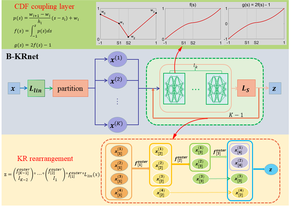
Figure 1: The schematic of B-KRnet. The input is passed to a linear layer that maps input into $[-1,1]^{d}$. Then divide it into $K$ parts and pass it to $K-1$ outer loops. Each outer loop $f^{outer}_{[k]}$ consists of $l_{k}$ non-linear mappings which are motivated by CDFs.

The definition of the CDF coupling layer and the specific choices given by equation (2.22) are based on the following considerations: First, CDF coupling layer can be relatively simple, meaning that we do not have to consider a very fine mesh on $[-1,1]^{d}$. It is seen that in the regular KRnet, the affine coupling layer simply defines a linear mapping for the data to be updated. Second, we rescale the data to the domain $[-1,1]^{d}$ to take advantage of the symmetry in terms of the origin, which is consistent with the initialization of the model parameters of the neural network around zero. Third, in equation (2.22) we use a tangent hyperbolic function to control the conditioning of the mapping such that neither $s_{i}$ (adaptive mesh grids) or $w_{i}$ (PDF on grids) vary too much to make the problem ill-posed.

The detailed schematic of our B-KRnet is shown in Fig. 1. The structure of B-KRnet is similar to KRnet [20] defined on an unbounded domain. The scale and bias layer of KRnet has been removed in B-KRnet since the domain is bounded. Another difference is that B-KRnet based on the CDF coupling layer will result in a PDF model that is piecewisely linear. If such a PDF model is used to approximate a second-order differential equation, e.g., the Fokker-Planck equation, a mixed formulation must be used, in other words, the gradient of the solution should be approximated by a separate neural network.

2.2 The complexity of B-KRnet

In this part, we discuss the degrees of freedom (DOFs) of B-KRnet, which is composed by $K-1$ mappings $f^{outer}_{[k]}$. Notice that all trainable parameters come from the CDF coupling layer. Each $f^{outer}_{[k]}$ includes $l_{k}$ CDF coupling layers. Then the number of DOFs of B-KRnet is

$$\text{DOFs}(p_{\text{B-KRnet},\bm{\theta}})=\sum_{k=1}^{K-1}\text{DOFs}(f^{outer}_{[k]})=\sum_{k=1}^{K-1}\sum_{i=1}^{l_{k}}\text{DOFs}(L_{CDF,[k,i]}).$$ (2.24)

For simplicity, let $K=d$. On the other hand, a portion of input dimensions will be deactivated through squeezing layer, suggesting simpler neural network $f^{outer}_{[k]}$ as $k$ increases. The most straightforward idea is to reduce the depth $l_{k}$ and width of hidden layer. Assume that neural network (2.21) in CDF coupling layer is fully connected and has two hidden layers, each with $w_{k}$ neurons. The input dimension of $L_{CDF,[k,i]}$ is $d-k+1$. Let $d_{i}<d-k+1$ denotes the input dimension of $\text{NN}(\cdot)$ defined by (2.21) for $L_{CDF,[k,i]}$. Then

$$\text{DOFs}(L_{CDF,[k,i]})+\text{DOFs}(L_{CDF,[k,i+1]})$$ (2.25)

$$= ~{}w_{k}d_{i}+w_{k}+w_{k}^{2}+w_{k}+6w_{k}(d-k+1-d_{i})+6(d-k+1-d_{i})$$

$$+w_{k}(d-k+1-d_{i})+w_{k}+w_{k}^{2}+w_{k}+6w_{k}d_{i}+6d_{i}$$

$$= ~{}2w_{k}^{2}+(7w_{k}+6)(d-k+1)+4w_{k}.$$

Substituting equation (2.25) into equation (2.24), we can obtain the total number of model parameters is

$$DOFs(p_{\text{B-KRnet},\bm{\theta}})=\sum_{i=1}^{d}\frac{l_{k}}{2}\big{(}2w_{k}^{2}+(7w_{k}+6)(d-k+1)+4w_{k}\big{)}.$$ (2.26)

3 Application to density estimation

Let $\bm{X}$ be a $d$-dimensional random variable with an unknown density function $p_{\bm{X}}(\cdot)$ defined on bounded domain $\Omega$. Given the observations $\{\bm{x}_{i}\}_{i=1}^{N}$ that are drawn independently from $p_{\bm{X}}$, we aim to construct a generative model which is able to approximate the distribution as well as generate samples to surrogate the target PDF. We then train the B-KRnet model to minimize the cross entropy between the data distribution and $p_{\text{B-KRnet}}$

$$\mathcal{L}_{data} =-\frac{1}{N}\sum_{i=1}^{N}\log(p_{\text{B-KRnet}}(\bm{x}_{i})),$$ (3.1)

$$=-\frac{1}{N}\sum_{i=1}^{N}\log\big(p_{\bm{Z}}\left(f_{\text{B-KRnet}}(\bm{x})\right)\big{missing})+\log\left(\left|\nabla_{\bm{x}}f_{\text{B-KRnet}}(\bm{x})\right|\right),$$

which is equivalent to maximizing the likelihood. Noting that the Kullback-Leibler (KL) divergence between $p_{\bm{X}}$ and the density model $p_{\text{B-KRnet}}$ can be written as

$$D_{\text{KL}}(p_{\bm{X}}\mid\mid p_{\text{B-KRnet}}) =-H(p_{\bm{X}})+H(p_{\bm{X}},p_{\text{B-KRnet}})$$ (3.2)

and

$$H(p_{\bm{X}},p_{\text{B-KRnet}})\approx-\frac{1}{N}\sum_{i=1}^{N}\log(p_{\text{B-KRnet}}(\bm{x}_{i}))=\mathcal{L}_{data},$$ (3.3)

where $\bm{x}_{i}$ are drawn from $p_{\bm{X}}$, $H(p_{\bm{X}})$ is the entropy of $p_{\bm{X}}$ and $H(p_{\bm{X}},p_{\text{B-KRnet}})$ is the cross entropy between $p_{\bm{X}}$ and $p_{\text{B-KRnet}}$, we are actually trying to minimize $D_{\text{KL}}(p_{\bm{X}}\mid\mid p_{\text{B-KRnet}})$ since the model is not related to $H(p_{\bm{X}})$.

To evaluate the accuracy of $p_{\text{B-KRnet}}$, we approximate the relative KL divergence by applying the Monte Carlo method on a validation set, i.e.,

$$\frac{D_{\mathrm{KL}}(p_{\bm{X}}\mid\mid p_{\text{B-KRnet}})}{H(p_{\bm{X}})}\approx\frac{\sum_{i=1}^{N_{v}}\big{(}\log(p_{\bm{X}}(\bm{x}_{i})-\log p_{\text{B-KRnet}}(\bm{x}_{i}))\big{)}}{-\sum_{i=1}^{N_{v}}\log p_{\bm{X}}(\bm{x}_{i})}.$$

Here $\bm{x}_{i}$ are drawn from the ground truth $p_{\bm{X}}$.

3.1 Example 1: Annulus

We consider an annulus,

$$\left\{\enspace\begin{aligned} &x=r\cos\theta,\\ &y=r\sin\theta,\\ &\theta\sim\text{Uniform}[0,2\pi],\quad r\sim f(r)=\frac{1}{r}1_{[1,\,e]},\end{aligned}\right.$$ (3.4)

where $1_{[1,\,e]}$ is an indicator function with $1_{[1,\,e]}(r)=1$ if $r\in 1_{[1,\,e]};\;0$ otherwise. $r$ can be sampled via $\log r\sim\text{Uniform}[0,1].$ That is to say, given a sample $\tilde{r}$ generated from a uniformly distributed on $[0,1]$, then $r=\exp(\tilde{r})$ obeys the PDF $f(r)$. Denote the domain constructed by $r$ and $\theta$ by $\Omega$. The ground truth PDF $p(x,y)$ has a form

$$p(x,y)=p(r,\theta)\left|\frac{\partial(x,y)}{\partial(r,\theta)}\right|^{-1}=\frac{1}{2\pi r^{2}}=\frac{1}{2\pi(x^{2}+y^{2})},\quad(x,y)\in\Omega.$$ (3.5)

The number of training points is $2\times 10^{4}$. For the B-KRnet, we take $8$ CDF coupling layers. The neural network introduced in (2.21) has two fully connected hidden layers with $32$ hidden neurons. The hyperbolic tangent function is used as activation function. The Adam method with an initial learning rate $0.001$ and batch size $4096$ is applied. A total of $4000$ epochs are considered and a validation dataset with $2\times 10^{4}$ samples is used for computing relative KL divergence during the whole training process.

Note that for this case, the entropy of $p$ is

$$H(p)=-\int_{1}^{e}\int_{0}^{2\pi}p(r,\theta)\log p(r,\theta)\mathrm{d}\theta\mathrm{d}r=-\int_{1}^{e}\int_{0}^{2\pi}\frac{1}{2\pi r}\log\left(\frac{1}{2\pi r}\right)\mathrm{d}\theta\mathrm{d}r=\frac{1}{2}+\log(2\pi).$$ (3.6)

The training loss and the relative KL divergence are presented in Fig. 2. We also compare the samples from the true distribution and samples from PDF model in Fig. 3. The samples generated by B-KRnet agree very well with the true samples. In particular, the sharp boundary of $p(x,y)$ is well captured.

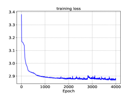
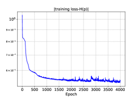
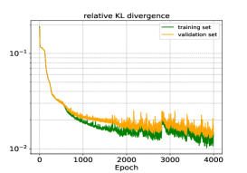
Figure 2: Training procedure for the distribution on an annulus. Left: The training loss. Middle: The KL divergence on the training set. Right: The relative KL divergence on the training set and validation set.

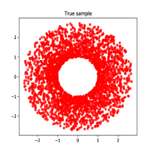
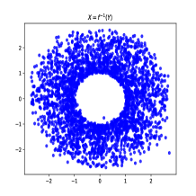
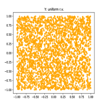
Figure 3: Comparison between true samples and samples from B-KRnet for the distribution on an annulus. Left: True samples. Middle: Samples from B-KRnet. Right: Samples from the prior (uniform).

3.2 Example 2: Mixture of Gaussians

We consider the portion of a mixture of Gaussians

$$p_{\bm{Y}}(\bm{y})=\frac{1}{6C}\sum\limits_{i=1}^{6}{N}(\bm{y}_{i},\sigma^{2}\bm{I}_{2})1_{[-1,1]^{2}}(\bm{y}),$$ (3.7)

that is located in $[-1,1]^{2}$, where $\bm{y}_{i}=(0.8\cos\frac{i\pi}{3}+0.3,0.8\sin\frac{i\pi}{3}+0.3)$, $\sigma=0.15$, $1_{[-1,1]^{2}}(\bm{y})$ is an indicator function,

$${N}(\bm{\mu},\bm{\Sigma}_{d})=\frac{1}{(2\pi)^{d/2}\det|\bm{\Sigma}|}\exp\left(-\frac{1}{2}(\bm{x}-\bm{\mu})^{\mathrm{T}}\bm{\Sigma}^{\mathrm{-1}}(\bm{x}-\bm{\mu})\right),$$

and $C$ is a normalization constant,

$$C=\int_{[-1,1]^{2}}\frac{1}{6}\sum\limits_{i=1}^{6}{N}(\bm{y}_{i},\sigma^{2}\bm{I})(\bm{y})d\bm{y}\approx\frac{4}{6M}\sum^{M}_{j}\sum_{i=1}^{6}{N}(\bm{y}_{i},\sigma^{2}\bm{I})(\bm{y}^{j}).$$ (3.8)

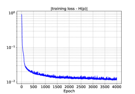
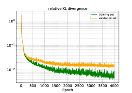
Figure 4: Training procedure for the mixture of Gaussians on a box. Left: The training loss. Middle: The KL divergence on the training set. Right: The relative KL divergence on the training set and validation set.

The configuration of B-KRnet is the same as the previous example. We obtain the approximation of $H(p)$ by generating $10^{6}$ samples from the true distribution. The training loss and the relative KL divergence are presented in Fig. 4. We also compare the samples from the true distribution and samples from the PDF model in Fig. 5. The B-KRnet model yields an excellent agreement with the ground truth distribution.

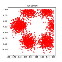
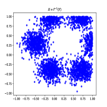
Figure 5: Comparison between true samples and samples from B-KRnet for the mixture of Gaussians on a box. Left: True samples. Middle: Samples from B-KRnet. Right: Samples from the prior (uniform).

3.3 Example 3: Logistic distribution with holes

We now consider density estimation for a logistic distribution with holes on a bounded domain $\Omega=[-10,10]^{d}$. The training dataset $S=\{\bm{y}^{(i)}\}^{N}_{i=1}$ is generated from $p_{\bm{Y}}(\bm{y})$, where the components of $\bm{Y}=(Y_{1},Y_{2},\dots,Y_{d})$ are i.i.d and each component $Y_{i}\sim$Logistic$(0,s)$ with PDF $\rho(y_{i};0,s)$. We constraint $\bm{Y}$ to $[-10,10]^{d}$ and require it also satisfies

$$\big{\|}R_{\gamma,\theta_{j}}[y_{j}^{(i)},y^{(i)}_{j+1}]^{\rm{T}}\big{\|}_{2}\geq C,\quad j=1,\dots,d-1,$$ (3.9)

where $C$ is a specified constant, and

$$\|R_{\gamma,\theta_{j}}\|=\left[\begin{array}[]{cc}\gamma&0\\ 0&1\\ \end{array}\right]\left[\begin{array}[]{cc}\cos\theta_{j}&-\sin\theta_{j}\\ \sin\theta_{j}&\cos\theta_{j}\\ \end{array}\right],\quad\theta_{j}=\left\{\begin{array}[]{cc}\frac{\pi}{4},&\text{ if }j\text{ is even; }\\ \frac{3\pi}{4},&\text{otherwise}.\end{array}\right.$$ (3.10)

Then an elliptic hole is generated for two adjacent dimensions. The reference PDF takes the form

$$p_{\bm{Y}}(\bm{y})=\frac{1_{B}(\bm{y})\prod_{i=1}^{d}\rho(y_{i};0,s)}{\mathbb{E}[1_{B}(\bm{Y})]},$$ (3.11)

where $B\subset\Omega$ is the domain admitting constraint (3.9), and $1_{B}(\cdot)$ is an indicator function with $1_{B}(y)=1$ if $\bm{y}\in B;\;0$ otherwise.

We set $d=8$, $C=5$, $\gamma=3$ and $s=2$. To demonstrate the effectiveness of the block-triangular model structure, we compare the performance of B-KRnet models subject to either KR rearrangement or the half-half partition used by classical flow-based models. For the sake of convenience, we call the latter Classical-NF. In fact, Classical-NF can be considered as $f^{outer}_{[1]}\circ L_{lin}$. In B-KRnet, we deactivate the dimensions by one, i.e., $K=8$. We let $l_{k}=l_{k-1}-2$ if $l_{k-1}\geq 6$ and $l_{1}=16$. The neural network defined by equation (2.21) consists of two fully connected hidden layers with $32$ hidden neurons. Notice that there is no outer loop for the Classical-NF. To match the DOFs of B-KRnet, we take $18$ CDF coupling layers with $64$ hidden neurons for Classical-NF. $10^{6}$ training points are considered. The batch size is set to $2\times 10^{5}$. The Adam optimizer with an initial learning rate $0.001$ is applied. Moreover, we adjust the learning rate to half of the initial learning rate after each $5000$ epochs. A total of $10000$ epochs are conducted and a validation dataset with $10^{6}$ samples is used for computing relative KL divergence throughout the training process.

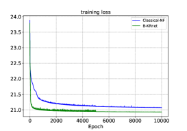
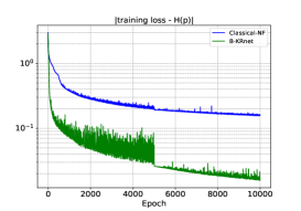
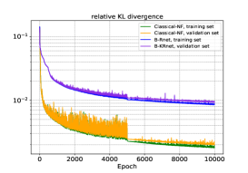
Figure 6: Comparison between Classical-NF and B-KRnet for $d=8$. Left: The training loss. Middle: The KL divergence on training set. Right: The relative KL divergence on training set and validation set.

The training loss and relative KL divergence are presented in Fig. 6, which indicate that KR rearrangement achieves higher accuracy than the half-half partition. We also compare the samples from the true distribution and samples from PDF models in Fig. 7. The samples generated from B-KRnet show a better agreement with the true samples than Classical-NF.

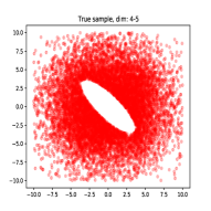
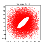
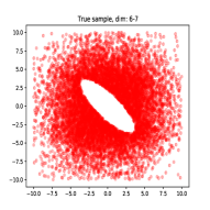
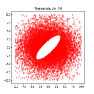
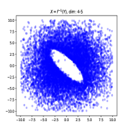
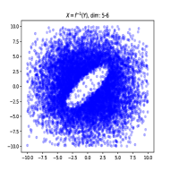
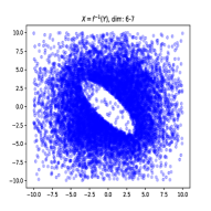
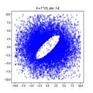
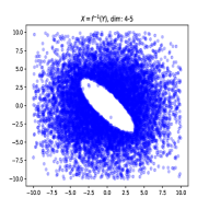
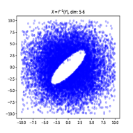
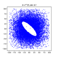
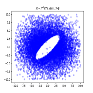
Figure 7: Comparison between true samples and samples from PDF models for $d=8$. Top: True samples. Middle: Samples from Classical-NF. Right: Samples from B-KRnet.

4 Application to solving PDEs on a bounded domain

In this part, we employ B-KRnet to approximate PDEs for density and elaborate the adaptive learning procedure in detail. Let $\Omega\subset\mathbb{R}^{d}$ be a hyperrectangle domain and $\bm{p}:\Omega\to\mathbb{R}_{+}$. We consider the following general PDE

$$\left\{\,\begin{aligned} \mathcal{N}[\bm{x};p(\bm{x})]=0,&\quad\bm{x}\in\Omega,\\ \mathcal{B}[\bm{x};p(\bm{x})]=0,&\quad\bm{x}\in\partial\Omega,\end{aligned}\right.$$ (4.1)

where $\mathcal{N}$ is a linear or nonlinear partial differential operator in terms of $\bm{x}$ and $\mathcal{B}$ is a boundary operator. We assume that the solution $p(\bm{x})$ is mass conservative, which is very common in physical and biological modeling. For simplicity, we regard $p$ as a PDF, i.e.,

$$\int_{\Omega}{p}(\bm{x}){\rm{d}}\bm{x}=1,\quad{p}(\bm{x})\geq 0,\quad\bm{x}\in\Omega.$$ (4.2)

We map $\bm{X}$ to a random vector $\bm{Z}$ which is uniformly distributed on $[-1,1]^{d}$ by B-KRnet and use the induced density model $p_{\text{B-KRnet},\bm{\theta}}(\bm{x})$ as a surrogate for $p(\bm{x})$. Since $p_{\text{B-KRnet},\bm{\theta}}$ is a PDF, the non-negativity and conservation constraints (4.2) naturally hold. Note that B-KRnet is limited to first-order differentiation since the CDF coupling layer is piecewise quadratic. To deal with a second-order PDE, we convert it into a first-order system by introducing an auxiliary vector function to represent the gradient $\nabla p$.

4.1 Tackle second order differential operator: auxiliary function

We rewrite equation (4.1) as a first-order system

$$\left\{\,\begin{aligned} \mathcal{N}[\bm{x};{p},\bm{g}]=0,&\quad\bm{x}\in\Omega,\\ \mathcal{B}[\bm{x};p,\bm{g}]=0,&\quad\bm{x}\in\partial\Omega,\\ \bm{g}=\nabla p,&\quad\bm{x}\in\Omega.\end{aligned}\right.$$ (4.3)

We employ a neural network $\bm{g}_{\text{NN}}$ to approximate $\bm{g}$. Following the physics-informed neural networks (PINNs), we consider the loss,

$$\mathcal{L}(p_{\text{B-KRnet},\bm{\theta}},\bm{g}_{\text{NN}})=\lambda_{{pde}}\mathcal{L}_{{pde}}(p_{\text{B-KRnet},\bm{\theta}},\bm{g}_{\text{NN}})+\lambda_{b}\mathcal{L}_{b}(p_{\text{B-KRnet},\bm{\theta}},\bm{g}_{\text{NN}})+\lambda_{\bm{g}}\mathcal{L}_{\bm{g}}(p_{\text{B-KRnet},\bm{\theta}},\bm{g}_{\text{NN}}),$$ (4.4)

where $\{\lambda_{pde},\lambda_{b},\lambda_{\bm{g}}\}$ are hyperparameters to balance the losses $\mathcal{L}_{pde}(p_{\text{B-KRnet},\bm{\theta}},\bm{g}_{\text{NN}})$, $\mathcal{L}_{b}(p_{\text{B-KRnet},\bm{\theta}},\bm{g}_{\text{NN}})$ and $\mathcal{L}_{\bm{g}}(p_{\text{B-KRnet},\bm{\theta}},\bm{g}_{\text{NN}})$ induced by the governing equations, the boundary conditions and $\bm{g}_{\text{NN}}$ respectively. More specifically,

$$\mathcal{L}_{pde}(p_{\text{B-KRnet},\bm{\theta}},\bm{g}_{\text{NN}})=\mathbb{E}_{\bm{x}\sim\rho}\big{[}\left|\mathcal{N}[\bm{x};p_{\text{B-KRnet},\bm{\theta}},\bm{g}_{\text{NN}}]\right|^{2}\big{]},$$ (4.5)

$$\mathcal{L}_{b}(p_{\text{B-KRnet},\bm{\theta}},\bm{g}_{\text{NN}})=\mathbb{E}_{\bm{x}\sim\rho_{b}}\big{[}\left|\mathcal{B}[\bm{x};p_{\text{B-KRnet},\bm{\theta}},\bm{g}_{\text{NN}}]\right|^{2}\big{]},$$ (4.6)

$$\mathcal{L}_{\bm{g}}(p_{\text{B-KRnet},\bm{\theta}},\bm{g}_{\text{NN}})=\mathbb{E}_{\bm{x}\sim\rho}\big{[}\left\|\bm{g}_{\text{NN}}(\bm{x})-\nabla p_{\text{B-KRnet},\bm{\theta}}(\bm{x})\right\|^{2}_{2}\big{]},$$ (4.7)

where $\rho(\bm{x})$ and $\rho_{b}(\bm{x})$ are positive PDFs on $\Omega$ and $\partial\Omega$ respectively. Given training data $C_{pde}=\{\bm{x}^{i}\}_{i=1}^{N_{pde}}$, $C_{b}=\{\bm{x}_{b}^{i}\}_{i=1}^{N_{b}}$, i.e., random samples of $\rho(\bm{x})$ and $\rho_{b}(\bm{x})$, the losses $\mathcal{L}_{pde}$, $\mathcal{L}_{b}$ and $\mathcal{L}_{\bm{g}}$can be approximated as

$$\mathcal{L}_{pde}(p_{\text{B-KRnet},\bm{\theta}},\bm{g}_{\text{NN}})\approx\widehat{\mathcal{L}}_{pde}(p_{\text{B-KRnet},\bm{\theta}},\bm{g}_{\text{NN}})\coloneqq\frac{1}{N_{pde}}\sum_{i=1}^{N_{pde}}\big{(}\mathcal{N}[\bm{x}^{i};p_{\text{B-KRnet},\bm{\theta}}(\bm{x}^{i}),\bm{g}_{\text{NN}}(\bm{x}^{i})]\big{)}^{2},$$ (4.8)

$$\mathcal{L}_{b}(p_{\text{B-KRnet},\bm{\theta}},\bm{g}_{\text{NN}})\approx\widehat{\mathcal{L}}_{b}(p_{\text{B-KRnet},\bm{\theta}},\bm{g}_{\text{NN}})\coloneqq\frac{1}{N_{b}}\sum\limits_{i=1}^{N_{b}}\big{(}\mathcal{B}[\bm{x}_{b}^{i};p_{\text{B-KRnet},\bm{\theta}}(\bm{x}^{i}_{b}),\bm{g}_{\text{NN}}(\bm{x}^{i}_{b})]\big{)}^{2},$$ (4.9)

$$\mathcal{L}_{\bm{g}}(p_{\text{B-KRnet},\bm{\theta}},\bm{g}_{\text{NN}})\approx\widehat{\mathcal{L}}_{\bm{g}}(p_{\text{B-KRnet},\bm{\theta}},\bm{g}_{\text{NN}})\coloneqq\frac{1}{N_{pde}}\sum\limits_{i=1}^{N_{pde}}\big{\|}\bm{g}_{\text{NN}}(\bm{x}^{i})-\nabla p_{\text{B-KRnet},\bm{\theta}}(\bm{x}^{i})\big{\|}^{2}_{2},$$ (4.10)

from which we define the total empirical loss $\widehat{\mathcal{L}}(p_{\text{B-KRnet},\bm{\theta}},\bm{g}_{\text{NN}})$ as

$$\widehat{\mathcal{L}}(p_{\text{B-KRnet},\bm{\theta}},\bm{g}_{\text{NN}}) =\lambda_{{pde}}\widehat{\mathcal{L}}_{{pde}}(p_{\text{B-KRnet},\bm{\theta}},\bm{g}_{\text{NN}})+\lambda_{b}\widehat{\mathcal{L}}_{b}(p_{\text{B-KRnet},\bm{\theta}},\bm{g}_{\text{NN}})+\lambda_{\bm{g}}\widehat{\mathcal{L}}_{\bm{g}}(p_{\text{B-KRnet},\bm{\theta}},\bm{g}_{\text{NN}}).$$ (4.11)

The optimal parameters $\bm{\theta}^{*}$ can be obtained via minimizing $\widehat{\mathcal{L}}(p_{\text{B-KRnet},\bm{\theta}},\bm{g}_{\text{NN}})$, i.e.,

$$\bm{\theta}^{*}=\arg\min_{\bm{\theta}}\widehat{\mathcal{L}}(p_{\text{B-KRnet},\bm{\theta}},\bm{g}_{\text{NN}}).$$ (4.12)

4.2 Adaptive sampling procedure

The choice of training points plays an important part in achieving good numerical accuracy. We pay particular attention to the choice of $C_{pde}$ here. Typically, the training points are generated from a uniform distribution on a finite domain $\Omega$ which is inefficient when $p(\cdot)$ is concentrated in a small (yet known) region. Recently, adaptive sampling procedures have been successfully applied to solve Fokker-Planck equations defined on the whole domain [23, 24, 25]. Noting that the residual $\left|\mathcal{N}[\bm{x};p_{\text{B-KRnet},\bm{\theta}},\bm{g}_{NN}]\right|$ is larger more likely in the region of high probability density, their choice for $\rho$ in equation (4.5) is $p_{\text{B-KRnet},\bm{\theta}}$, which also takes advantage of the fact that flow-based models can generate exact samples easily. We adopt a similar procedure to solve PDEs on bounded domains.

The crucial idea is to update the training set by samples from the current optimal B-KRnet and then continue the training process. Since we have no prior knowledge of the solution at the beginning, we let $\rho$ be a uniform distribution, i.e., the initial set of collocation points $C_{pde}$ are drawn from a uniform distribution in $\Omega$. $C_{b}$ is also drawn from a uniform distribution on $\partial\Omega$. Then we solve the optimization problem (4.12) via the Adam optimizer and obtain optimal $\bm{\theta}^{*,0}$, which corresponds to a bounded mapping $f_{\bm{\theta}^{*,0}}$ and a PDF $p_{\text{B-KRnet},\bm{\theta}^{*,0}}$. We update part of the collocation points in $C_{pde}$ by drawing samples from $p_{\text{B-KRnet},\bm{\theta}^{*,0}}$, i.e., update $\rho=(1-\gamma)\rho+\gamma p_{\text{B-KRnet},\bm{\theta}^{*,0}}$ where $0<\gamma\leq 1$. More specifically, we form the new training set $C_{pde}^{1}$ using the current training set and samples from $\bm{X}=(f_{\bm{\theta}^{*,0}})^{\rm{-1}}(\bm{Z})$ according to a mixture distribution, where $\bm{Z}$ is an uniform random variable. Then we continue to train the B-KRnet with $C_{pde}^{1}$ and $C_{b}$ to obtain the optimal $\bm{\theta}^{*,1}$. Repeat this procedure until the maximum number of updates is reached. In this way, more collocation points will be chosen in the region of higher density while fewer collocation points in the region of lower density. Such a strategy can be concluded as follows.

1. Let $\rho(\bm{x})=\frac{1}{|\Omega|}$. Generate an initial training set with samples uniformly distributed in $\Omega$:

   $$C_{pde}^{0}=\{\bm{x}^{i,0}\}_{i=1}^{N_{pde}}\subset\Omega,\quad\bm{x}^{i,0}\sim{\mathrm{Uniform}}\;\Omega,$$

   $$C_{b}=\{\bm{x}^{i}_{b}\}_{i=1}^{N_{b}}\subset\partial\Omega,\quad\bm{x}^{i}_{b}\sim{\mathrm{Uniform}}\;\partial\Omega.$$

2. Train B-KRnet by solving optimization problem (4.12) with training datasets $C_{pde}^{0}$ and $C_{b}$ to obtain $\bm{\theta}^{*,0}$.

3. $\rho(\bm{x})=(1-\gamma)\rho(\bm{x})+\gamma p_{\text{B-KRnet},\bm{\theta}^{*,0}}(\bm{x})$, $N_{new}=\gamma*N_{pde}$. Generate samples from $p_{\text{B-KRnet},\bm{\theta}^{*,0}}(\cdot)$ to get a new training set $C_{pde}^{1}=\{\bm{x}^{i,1}\}_{i=1}^{N_{new}}$. The new collocation point $\bm{x}^{i,1}$ can be obtained by transforming the prior uniformly distributed sample via the inverse normalizing flow,

   $$\bm{z}^{i,1}\sim\mathrm{Uniform}(-1,1)^{d},\quad\bm{x}^{i,1}=\big{(}f_{\bm{\theta}^{*,0}}\big{)}^{\rm{-1}}(\bm{z}^{i,1}).$$

   Set $C_{pde}^{0}=C_{pde}^{1}\cup\{\bm{x}^{i,0}\}_{i=N_{new}+1}^{N_{pde}}$.

4. Repeat steps 2-3 for $N_{\mathrm{adaptive}}$ times to get a convergent approximation.

Our algorithm is summarized in Algorithm 1.

Algorithm 1 Solving PDEs involving density

Input: maximum epoch number $N_{e}$, maximum iteration number $N_{\mathrm{adaptive}},$ update rate $\gamma$, initial training data $C_{pde}=\{\bm{x}^{i}\}_{i=1}^{N_{pde}}$, $C_{b}=\{\bm{x}^{i}_{b}\}_{i=1}^{N_{b}}$, initial learning rate $l_{r}$, decay rate $\eta$, step size $n_{s}$.

for $k=0,\cdots,N_{\mathrm{adaptive}}$ do

     for $j=1,\cdots,N_{e}$ do

         Divide $C_{pde}$, $C_{b}$ into $n$ mini-batches $\{C^{ib}_{pde}\}_{ib=1}^{n}$, $\{C^{ib}_{b}\}_{ib=1}^{n}$ randomly.

         for $ib=1,\cdots,n$ do

              if $((k-1)N_{e}+j)\%n_{s}==0$ then

                  $l_{r}=\eta*l_{r}$.               end if

              Compute the loss function (4.11) ${\widehat{\mathcal{L}}^{ib}}(p_{\text{B-KRnet},\bm{\theta}},\bm{g}_{\text{NN}})$ for mini-batch data $C^{ib}_{pde}$ and $C^{ib}_{b}$,

              Update $\bm{\theta}$ by using the Adam optimizer.          end for      end for

     $N_{new}=\gamma*N_{pde}$. Sample from $p_{\text{B-KRnet},\bm{\theta}}(\cdot)$ and update training set $C_{pde}$. end for

Output: The predicted solution $p_{\text{KRnet},\bm{\theta}}(\bm{x})$.

5 Application to solving PDEs over mixed domains

In practical applications, we often encounter mixed regions. For example, the solution of kinetic Fokker-Planck equation is a PDF of location and velocity, where in general the location is bounded and the velocity is unbounded. We consider the following PDE,

$$\left\{\,\begin{aligned} &\mathcal{N}[\bm{x},\bm{v};p(\bm{x},\bm{v})]=f(\bm{x},\bm{v}),\quad\bm{x}\in\Omega,\quad\bm{v}\in\mathbb{R}^{d},\\ &\mathcal{B}[\bm{x},\bm{v};p(\bm{x},\bm{v})]=0,\qquad\quad\bm{x}\in\partial\Omega,\quad\bm{v}\in\mathbb{R}^{d},\end{aligned}\right.$$ (5.1)

where $p(\bm{x};\bm{v})$ is assumed to be a PDF. To deal with problems defined on mixed regions, we develop a conditional flow which combines the original KRnet and B-KRnet.

For $\bm{v}\in\mathbb{R}^{d}$, $d>1$, and $\bm{x}\in\Omega$, we rewrite the PDF as

$$p(\bm{x},\bm{v})=h(\bm{v}|\bm{x})\cdot q(\bm{x}),$$ (5.2)

where $q(\bm{x})$ denotes the marginal distribution of spatial variable $\bm{x}$ and $h(\bm{v}|\bm{x})$ denotes the probability of velocity $\bm{v}$ at the position $\bm{x}$. We model $q(\bm{x})$ by B-KRnet and $h(\bm{v}|\bm{x})$ by original KRnet, i.e.,

$$p_{\bm{\theta}}(\bm{x},\bm{v})=h_{\text{KRnet},\bm{\theta}_{1}}(\bm{v}|\bm{x})\cdot q_{\text{B-KRnet},\bm{\theta}_{2}}(\bm{x}).$$ (5.3)

The construction of the conditional probability model $h_{\text{KRnet},\bm{\theta}_{1}}(\bm{v}|\bm{x})$ can be down by the similar way of [24]. The only difference is that the conditional probability in [24] is conditional on time, while here the location information is used as the condition. Following the similar discussion in Section 4.1, we can easily derive the loss function for problem (5.1). We can also use the procedure described in Section 4.2 to develop an adaptive sampling strategy.

6 Numerical results

In this section, we provide several numerical experiments to demonstrate the effectiveness of the proposed approach presented in Algorithm 1. We first present the performance of the methods to solve a four-dimensional problem and examine the performance of adaptive training. We then apply our method to the Keller-Segel equations which involve two PDFs. To further demonstrate the efficiency of B-KRnet, we combine B-KRnet and KRnet to solve the kinetic Fokker-Planck equation. We empoly the hyperbolic tangent function (Tanh) as the activation function. $\text{NN}(\bm{x}_{1})$ in equation (2.21) is a fully connected network with two hidden layers. The algorithms are implemented with Adam optimizer [41] in Pytorch where the initial learning rate is $0.001$. The update rate for a new training set is set to $\gamma=0.8$.

6.1 Four-dimensional test problem

We start with the following four-dimensional problem,

$$\left\{\enspace\begin{aligned} &-\Delta p(\bm{x})+p(\bm{x})=f(\bm{x}),\quad\bm{x}\in\Omega=(0,\pi)^{4},\\ &\quad\frac{\partial p(\bm{x})}{\partial\bm{n}}\bigg{|}_{\partial\Omega}=0,\\ &\int_{\Omega}p(\bm{x}){\rm d}\bm{x}=1,\quad p(\bm{x})\geq 0.\end{aligned}\right.$$ (6.1)

where $f(\bm{x})=\frac{8}{9\pi^{4}}(5\cos{x_{1}}\cos{x_{2}}\cos{x_{3}}\cos{x_{4}}+\frac{9}{8})$. The exact solution is $p(\bm{x})=\frac{8}{9\pi^{4}}(\cos{x_{1}}\cos{x_{2}}\cos{x_{3}}\cos{x_{4}}+\frac{9}{8})$. We introduce an auxiliary function $\bm{g}$ to represent the gradient of $p$ and rewrite the equation (6.1) as

$$\left\{\enspace\begin{aligned} &-\nabla\cdot\bm{g}(\bm{x})+p(\bm{x})=f(\bm{x}),\quad\bm{x}\in\Omega=(0,\pi)^{4},\\ &\bm{g}(\bm{x})\cdot\bm{n}(\bm{x})\big{|}_{\partial\Omega}=0,\\ &\nabla p(\bm{x})=\bm{g}(\bm{x}),\quad\bm{x}\in\Omega,\\ &\int_{\Omega}p(\bm{x}){\rm d}\bm{x}=1,\quad p(\bm{x})\geq 0.\end{aligned}\right.$$ (6.2)

In the framework of PINN, we approximate the gradient by neural network $\bm{g}_{\text{NN}}$ and solution $p$ by B-KRnet $p_{\text{B-KRnet},\bm{\theta}}$. To enforce $\bm{g}_{\text{NN}}$ to satisfy the Neumann boundary condition exactly, we consider the following surrogate

$$\bm{g}_{\text{NN}}(\bm{x})=\text{diag}(\bm{x}(\pi-\bm{x}))\tilde{\bm{g}}(\bm{x}),$$ (6.3)

where $\tilde{\bm{g}}_{NN}$ is a fully connected neural network whose specific structure is 2-64-32-32-32-2. Therefore the final loss function admits

$$\widehat{\mathcal{L}}(p_{\text{B-KRnet},\bm{\theta}})=\lambda_{pde}\widehat{\mathcal{L}}_{pde}(p_{\text{B-KRnet},\bm{\theta}})+\lambda_{\bm{g}}\widehat{\mathcal{L}}_{\bm{g}}(p_{\text{B-KRnet},\bm{\theta}}).$$ (6.4)

For the B-KRnet, we deactivate the dimensions by one., i.e., $K=4$ and let $l_{1}=8$, $l_{2}=l_{3}=l_{4}=6$. The neural network introduced in (2.21) has two fully connected hidden layers with $32$ hidden neurons. The number of epochs is $500$, and four adaptivity iterations are conducted. The Adam method with an initial learning rate $0.001$ is applied. After every 100 epochs, The learning rate is descreased by half every $500$ epochs. The number of training points is $4000$ and the batch size is $2000$. A validation dataset with $5\times 10^{4}$ samples is used for calculating the relative errors during the whole training process.

Fig. 8 records the results of training processes with and without adaptive sampling. From Fig. 8 and Fig. 8, we can observe that the relative error of adaptive B-KRnet is smaller than that of B-KRnet without adaptivity. Moreover, the convergence of B-KRnet is much faster. Fig. 8 plots the relative errors with respect to adaptivity iteration steps.

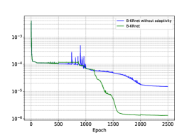
(a) The training loss

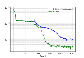
(b) The relative KL divergence

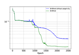
(c) The relative $L_{2}$ error of $p$

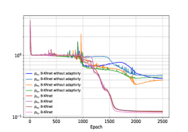
(d) The relative $L_{2}$ error of $\nabla p$

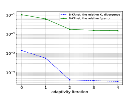
(e) The relative error w.r.t. adaptivity iteration step

Figure 8: Comparison between B-KRnet and B-KRnet without adaptivity for four-dimensional problem.

6.2 Stationary Keller-Segel system

We consider the following stationary Keller-Segel equation [42],

$$\left\{\enspace\begin{aligned} &\Delta u(\bm{x})-\nabla\cdot(u\nabla v)(\bm{x})+f(\bm{x})=0,&\bm{x}\in\Omega,\\ &-\Delta v(\bm{x})+v(\bm{x})=u(\bm{x}),&\bm{x}\in\Omega,\\ &\quad\frac{\partial u}{\partial\bm{n}}\bigg{|}_{\partial\Omega}=0,\quad\frac{\partial v}{\partial\bm{n}}\bigg{|}_{\partial\Omega}=0,\\ &\int_{\Omega}u(\bm{x}){\rm d}\bm{x}=1,\quad u(\bm{x})\geq 0,\quad\bm{x}\in\Omega,\\ &\int_{\Omega}v(\bm{x}){\rm d}\bm{x}=1,\quad v(\bm{x})\geq 0,\quad\bm{x}\in\Omega,\end{aligned}\right.$$ (6.5)

where $\Omega=(0,\pi)^{2}$, $\bm{x}=(x,y)$, $u(\bm{x})$ is the unknown density of some bacteria, $v(\bm{x})$ is the density of chemical attractant and

$$f(x,y)=\frac{1}{6\pi^{2}}\left(-4(-1+3\pi^{2})\cos x\cos y+\cos^{2}x(1+3\cos 2y)-2\cos^{2}y\sin^{2}x\right).$$

The corresponding true solution is

$$u(x,y)=\frac{1}{\pi^{2}}(\cos x\cos y+1),\quad v(x,y)=\frac{1}{3\pi^{2}}(\cos x\cos y+3).$$ (6.6)

In this case, two B-KRnets are required to represent $u$ and $v$ respectively. We introduce $\bm{\phi},\bm{\psi}$ to represent the derivative of $u,v$ respectively, i.e. $\bm{\phi}=\nabla u$, $\bm{\psi}=\nabla v$, and rewrite equation (6.5) as

$$\left\{\enspace\begin{aligned} &\nabla\cdot\bm{\phi}(\bm{x})-\nabla u(\bm{x})\cdot\nabla v(\bm{x})-(\nabla\cdot\bm{\psi})u(\bm{x})+f(\bm{x})=0,&\quad\bm{x}\in\Omega,\\ &-\nabla\cdot\bm{\psi}(\bm{x})+v(\bm{x})=u(\bm{x}),&\bm{x}\in\Omega,\\ &\quad\bm{\phi}\cdot\bm{n}\big{|}_{\partial\Omega}=0,\quad\bm{\psi}\cdot\bm{n}\big{|}_{\partial\Omega}=0,\\ &\bm{\phi}(\bm{x})=\nabla u(\bm{x}),\quad\bm{\psi}(\bm{x})=\nabla v(\bm{x}),\quad\bm{x}\in\Omega,\\ &\int_{\Omega}u(\bm{x}){\rm d}\bm{x}=1,\quad u(\bm{x})\geq 0,\quad\bm{x}\in\Omega,\\ &\int_{\Omega}v(\bm{x}){\rm d}\bm{x}=1,\quad v(\bm{x})\geq 0,\quad\bm{x}\in\Omega.\end{aligned}\right.$$ (6.7)

We use $\bm{\phi}_{\text{NN}}$ and $\bm{\psi}_{\text{NN}}$ to approximate $\bm{\phi}$ and $\bm{\psi}$ respectively, which are defined as

$$\bm{\phi}_{\text{NN}}(x,y)=\text{diag}(x(\pi-x),\,y(\pi-y))\widetilde{\bm{\phi}}_{\text{NN}}(x,y),\quad\bm{\psi}_{\text{NN}}(x,y)=\text{diag}(x(\pi-x),\,y(\pi-y))\widetilde{\bm{\psi}}_{\text{NN}}(x,y),$$ (6.8)

where $\widetilde{\bm{\phi}}_{NN}$ and $\widetilde{\bm{\psi}}_{NN}$ are both neural networks with four hidden layers, each with 32 neurons. Then our final loss function admits

$$\widehat{\mathcal{L}}(u_{\text{B-KRnet},\bm{\theta}_{1}},v_{\text{B-KRnet},\bm{\theta}_{2}},\bm{\phi}_{\text{NN}},\bm{\psi}_{\text{NN}})= \lambda_{pde,u}\widehat{\mathcal{L}}_{{pde,u}}(u_{\text{B-KRnet},\bm{\theta}_{1}})+\lambda_{\bm{\phi}}\widehat{\mathcal{L}}_{\bm{\phi}}(u_{\text{B-KRnet},\bm{\theta}_{1}},\bm{\phi}_{\text{NN}})$$ (6.9)

$$+\lambda_{pde,v}\widehat{\mathcal{L}}_{{pde,v}}(v_{\text{B-KRnet},\bm{\theta}_{2}})+\lambda_{\bm{\psi}}\widehat{\mathcal{L}}_{\bm{\psi}}(v_{\text{B-KRnet},\bm{\theta}_{2}},\bm{\psi}_{\text{NN}}),$$

where $\widehat{\mathcal{L}}_{\bm{\phi}}(u_{\text{B-KRnet},\bm{\theta}_{1}},\bm{\phi}_{\text{NN}})$ and $\widehat{\mathcal{L}}_{\bm{\psi}}(v_{\text{B-KRnet},\bm{\theta}_{2}},\bm{\psi}_{\text{NN}})$ are defined by equation (4.10).

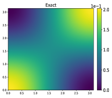
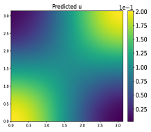
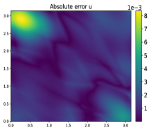
Figure 9: Comparison between true solution $u$ and numerical solution $u_{\text{B-KRnet},\bm{\theta}_{1}}$ of Keller-Segel equation. Left: The ground truth of $u$. Middle: Predicted solution $u_{\text{B-KRnet},\bm{\theta}_{1}}$. Right: $|u-u_{\text{B-KRnet},\bm{\theta}_{1}}|.$

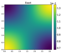
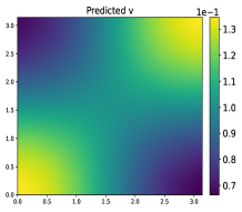
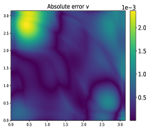
Figure 10: Comparison between true solution $v$ and numerical solution $v_{\text{B-KRnet},\bm{\theta}_{2}}$ of Keller-Segel equation. Left: The ground truth of $v$. Middle: Predicted solution $v_{\text{B-KRnet},\bm{\theta}_{2}}$. Right: $|v-v_{\text{B-KRnet},\bm{\theta}_{2}}|$.

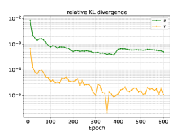
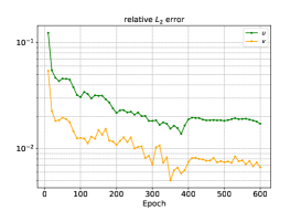
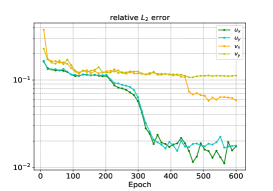
Figure 11: The relative error for Keller-Segel equation.

For the B-KRnet, we take $8$ affine coupling layers with $32$ hidden neurons. We use $2-64-32-32-32-2$ network for $\widetilde{\bm{\phi}}_{\text{NN}}$ and $\widetilde{\bm{\psi}}_{\text{NN}}$. $\lambda_{u}=\lambda_{v}=\lambda_{\bm{\phi}}=\lambda_{\bm{\psi}}=1$. We set batch size to $1024$ and the number of training points to $10^{4}$. The initial learning rate is $0.001$ with half decay each 200 epochs. Five adaptivity iterations with 100 epochs are conducted. A validation dataset with $10^{6}$ samples is used for calculating the relative errors during the whole training process. The comparison between the true solution and the predicted solution are presented in Fig. 9 and Fig. 10. The relative errors are presented in Fig. 11. The numerical solution provided by B-KRnet yields a good agreement with the analytic solution.

6.3 2D stationary kinetic Fokker-Planck equation

To illustrate the feasibility of the combination of KRnet and B-KRnet, we consider the following two-dimensional stationary kinetic Fokker-Planck equation with Dirichlet boundary conditions, i.e.,

$$\left\{\enspace\begin{aligned} &-\bm{v}\cdot\nabla_{\bm{x}}p+\nabla_{\bm{v}}\cdot(\sigma\nabla_{\bm{v}}p+\bm{v}p)=f,&(\bm{x},\bm{v})\in\Omega\times\mathbb{R}^{2},\\ &p(\bm{x},\bm{v})\big{|}_{\partial\Omega}=0,&\bm{v}\in\mathbb{R}^{2},\\ &\int_{\Omega\times\mathbb{R}}p(\bm{x},\bm{v})d\bm{x}d\bm{v}=1,~{}~{}p(\bm{x},\bm{v})\geq 0,&(\bm{x},\bm{v})\in\Omega\times\mathbb{R}^{2},\end{aligned}\right.$$ (6.10)

where $\Omega=(0,2)^{2}$, $f=\frac{p}{\sigma}\|\bm{x}+\bm{v}\|^{2}-\frac{9}{16\sigma\pi}((1-x_{1})x_{2}(2-x_{2})v_{1}-(1-x_{2})x_{1}(2-x_{1})v_{2})\exp(-\frac{\|\bm{v}+\bm{x}\|_{2}^{2}}{2\sigma}).$ The ground truth is

$$p(\bm{x},v)=\frac{9x_{1}x_{2}(2-x_{1})(2-x_{2})}{16\pi\sigma}\exp(-\frac{\|\bm{v}+\bm{x}\|_{2}^{2}}{2\sigma}).$$ (6.11)

We consider the case that $\sigma=4$. This system is of second order with respect to $\bm{v}$, but of first order with respect to $\bm{x}$. We approximate the unknown $p$ by formula (5.3). Then

$$\frac{\partial^{2}p_{\bm{\theta}}(\bm{x},\bm{v})}{\partial v_{i}v_{j}}=\frac{\partial^{2}h_{\text{KRnet},\bm{\theta}_{1}}(\bm{v}|\bm{x})}{\partial v_{i}v_{j}}\cdot q_{\text{B-KRnet},\bm{\theta}_{2}}(\bm{x}).$$

Since KRnet is second-order differentiable, we can directly obtain the loss function via PINN without converting the above system (6.10) into a first-order system.

The number of training points is set to $6\times 10^{4}$. The initial training points are drawn from a uniform distribution over $[0,2]^{2}\times[-5,5]^{2}$. For the B-KRnet and KRnet, we both take $8$ affine coupling layers with $32$ hidden neurons. The hyperparameters $\lambda_{pde}$ is set to $1$ and $\lambda_{b}$ is set to $10$. The Adam method and batch size $3000$ is applied. The initial learning rate is $0.0002$ with half decay each 400 epochs. The number of epochs is set to 1, and the number of adaptivity iterations conducted for this problem is set to $N_{\text{adaptive}}=500$. A validation dataset with $10^{6}$ samples is used for calculating the relative errors during the whole training process.

The comparison between the ground truth and the predicted solution at $\bm{x}=(0.5,0.5)$ and $\bm{x}=(1.8,1.8)$ are presented in Fig. 12. The training loss and the relative errors are presented in Fig. 13. We can observe that our method agrees well with the ground truth.

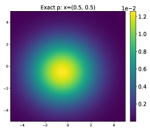
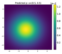
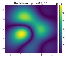
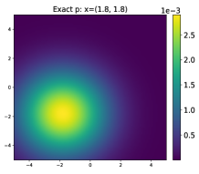
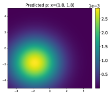
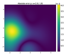
Figure 12: $\sigma=4$. Comparison between the predicted solutions and the reference solutions. Top row: $\bm{x}=(0.5,0.5)$. Bottom row: $\bm{x}=(1.8,1.8)$.

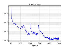
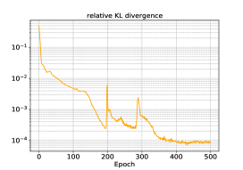
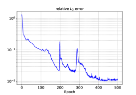
Figure 13: The training loss and the relative error for kinetic Fokker-Planck equation.

7 Conclusion

We have developed a bounded normalizing flow B-KRnet in this work, which can be regarded as a bounded version of KRnet. B-KRnet is build on a block-triangular structure whose core layer is CDF coupling layer. It models unknown PDF via mapping from target distribution to uniform distribution. Taking advantage of invertibility, B-KRnet could give a explicit PDF and generate samples from PDF easily as well. We apply B-KRnet to density estimation. The samples generated by B-KRnet show excellent agreement with the ground truth. Moreover, we develop an adaptive density approximation scheme for solving PDEs whose solutions are PDFs. A series of examples including a four-dimensional problem, a Keller-Segel equation and a kinetic Fokker-Planck equation is presented to demonstrate the efficiency of our method. There are, however, many important issues need to be addressed. The smoothness of B-KRnet is limited to first order. We convert the second-order system into first-order by introducing an auxiliary network to represent the gradient of PDF under the framework of PINNs. Actually, for some equations with variational forms, deep Ritz method shall be considered, which reformulates a PDE problem as a variational minimal problem without calculating the second-order derivative. How to update training points adaptively in the framework of deep Ritz deserves further discussion. In addition, we may consider other coupling layers to improve the smoothness and flexibility of bounded normalizing flow, which will be left for future study.

References

- Scott [1979] D. W. Scott, On optimal and data-based histograms, Biometrika 66 (1979) 605–610.
- Schwartz [1967] S. C. Schwartz, Estimation of probability density by an orthogonal series, The Annals of Mathematical Statistics (1967) 1261–1265.
- Yen-Chi [2017] C. Yen-Chi, A tutorial on kernal density estimation and recent advances, Biostatistics & Epidemiology 1 (2017) 161–187.
- Silverman [2018] B. W. Silverman, Density estimation for statistics and data analysis, Routledge, 2018.
- Jones [1993] M. C. Jones, Simple boundary correction for kernel density estimation, Statistics and computing 3 (1993) 135–146.
- Chen [1999] S. X. Chen, Beta kernel density estimations for density function, Computational Statistics & Data Analysis 31 (1999) 131–145.
- Kang et al. [2018] Y.-J. Kang, Y. Noh, O.-K. Lim, Kernel density estimation with bounded data, Structural and Multidisciplinary Optimization 57 (2018) 95–113.
- Bertin et al. [2019] K. Bertin, S. El Kolei, N. Klutchnikoff, Adaptive density estimation on bounded domains, in: Annales de 1’ Institut Henri Poincaré, volume 55, pp. 1916–1947.
- Goodfellow et al. [2020] I. Goodfellow, J. Pouget-Abadie, M. Mirza, B. Xu, D. Warde-Farley, S. Ozair, A. Courville, Y. Bengio, Generative adversarial networks, Communications of the ACM 63 (2020) 139–144.
- Kingma and Welling [2013] D. P. Kingma, M. Welling, Auto-encoding variational bayes, arXiv preprint arXiv: 1312.6114 (2013).
- Dinh et al. [2014] L. Dinh, D. Krueger, Y. Bengio, NICE: Non-linear independent components estimation, arXiv preprint arXiv:1410.8516 (2014).
- Dinh et al. [2016] L. Dinh, J. Sohl-Dickstein, S. Bengio, Density estimation using Real NVP, arXiv preprint arXiv:1605.08803 (2016).
- Kingma et al. [2016] D. P. Kingma, T. Salimans, R. Jozefowicz, X. Chen, I. Sutskever, M. Welling, Improved variational inference with inverse autoregressive flow, Advances in neural information processing systems 29 (2016).
- Papamakarios et al. [2017] G. Papamakarios, T. Pavlakou, I. Murray, Masked autoregressive flow for density estimation, Advances in neural information processing systems 30 (2017).
- Kingma and Dhariwal [2018] D. P. Kingma, P. Dhariwal, Glow: Generative flow with invertible 1x1 convolutions, Advances in neural information processing systems 31 (2018).
- Müller et al. [2019] T. Müller, B. McWilliams, F. Rousselle, M. Gross, J. Novák, Neural importance sampling, ACM Transactions on Graphics (ToG) 38 (2019) 1–19.
- Durkan et al. [2019a] C. Durkan, A. Bekasov, I. Murray, G. Papamakarios, Cubic-spline flows, arXiv preprint arXiv:1906.02145 (2019a).
- Durkan et al. [2019b] C. Durkan, A. Bekasov, I. Murray, G. Papamakarios, Neural spline flows, Advances in neural information processing systems 32 (2019b).
- Ho et al. [2019] J. Ho, X. Chen, A. Srinivas, Y. Duan, P. Abbeel, Flow++: Improving flow-based generative models with variational dequantization and architecture design, in: International Conference on Machine Learning, PMLR, pp. 2722–2730.
- Tang et al. [2020] K. Tang, X. Wan, Q. Liao, Deep density estimation via invertible block-triangular mapping, Theoretical and Applied Mechanics Letters 10 (2020) 143–148.
- Wan and Tang [2021] X. Wan, K. Tang, Augmented krnet for density estimation and approximation, arXiv preprint arXiv:2105.12866 (2021).
- Tang et al. [2023] K. Tang, X. Wan, C. Yang, DAS-PINNs: A deep adaptive sampling method for solving high-dimensional partial differential equations, Journal of Computational Physics 476 (2023) 111868.
- Tang et al. [2022] K. Tang, X. Wan, Q. Liao, Adaptive deep density approximation for fokker-planck equations, Journal of Computational Physics 457 (2022) 111080.
- Feng et al. [2022] X. Feng, L. Zeng, T. Zhou, Solving time dependent Fokker-Planck equations via temporal normalizing flow, Communication in Computational Physics (2022) 401–423.
- Zeng et al. [2022] L. Zeng, X. Wan, T. Zhou, Adaptive deep density approximation for fractional Fokker-Planck equations, arXiv preprint arXiv:2210.14402 (2022).
- Feng et al. [2023] Y. Feng, K. Tang, X. Wan, Q. Liao, Dimension-reduced krnet maps for high-dimensional inverse problems, arXiv preprint arXiv:2303.00573 (2023).
- Wan and Wei [2020] X. Wan, S. Wei, VAE-KRnet and its applications to variational bayes, arXiv preprint arXiv:2006.16431 (2020).
- Cercignani [1988] C. Cercignani, The Boltzmann equation, Springer, 1988.
- Keller and Segel [1970] E. F. Keller, L. A. Segel, Initiation of slime mold aggregation viewed as an instability, Journal of theoretical biology 26 (1970) 399–415.
- Golovnev and Trimper [2010] A. Golovnev, S. Trimper, Steady state solution of the poisson-nernst-planck equations, Physics Letters A 374 (2010) 2886–2889.
- Eisebverg [1998] B. Eisebverg, Ionic channels in biological membranes-electrostatic analysis of a natural nanotube, Contemporary Physics 39 (1998) 447–466.
- Corrias et al. [2004] L. Corrias, B. î. Perthame, H. Zaag, Global solutions of some chemotaxis and angiogenesis systems in high space dimensions, Milan Journal of Mathematics 72 (2004).
- Horstmann [2003] D. Horstmann, From 1970 until present: the Keller-Segel model in chemotaxis and its consequences, Jahresberichte DMV 105 (2003) 103–165.
- Yu et al. [2018] B. Yu, et al., The deep Ritz method: a deep learning-based numerical algorithm for solving variational problems, Communications in Mathematics and Statistics 6 (2018) 1–12.
- Raissi et al. [2019] M. Raissi, P. Perdikaris, G. E. Karniadakis, Physics-informed neural networks: A deep learning framework for solving forward and inverse problems involving nonlinear partial differential equations, Journal of Computational physics 378 (2019) 686–707.
- Zang et al. [2020] Y. Zang, G. Bao, Y. Xiaojing, H. Zhou, Weak adversarial networks for high-dimensional partial differential equations, Journal of Computional Physics 411 (2020) 109409.
- Yang et al. [2020] L. Yang, D. Zhang, G. E. Karniadakis, Physics-informed generative adversarial networks for stochastic differential equations, SIAM Journal on Scientific Computing 42 (2020) A292–A317.
- Yang and Perdikaris [2019] Y. Yang, P. Perdikaris, Adversarial uncertainty quantification in physics-informed neural networks, Journal of Computational Physics 394 (2019) 136–152.
- Guo et al. [2022] L. Guo, H. Wu, T. Zhou, Normalizing field flows: Solving forward and inverse stochastic differential equations using physics-informed flow models, Journal of Computational Physics 461 (2022) 111202.
- Dong et al. [2021] H. Dong, Y. Guo, T. Yastrzhembskiy, Kinetic Fokker-Planck and landau equations with specular reflection boundary condition, arXiv preprint arXiv:2111.09840 (2021).
- Kingma and Ba [2014] D. P. Kingma, J. Ba, Adam: A method for stochastic optimization, arXiv preprint arXiv:1412.6980 (2014).
- Hu and Zhang [2021] J. Hu, X. Zhang, Positivity-preserving and energy-dissipative finite difference schemes for the fokker-planck and keller-segel equations, arXiv preprint arXiv:2103.16790 (2021).