Identifying Disappearance of a White Dwarf Binary with LISA

Abstract

We discuss the prospect of identifying a white dwarf binary merger by monitoring disappearance of its nearly monochromatic gravitational wave. For a ten-year operation of the laser interferometer space antenna (LISA), the chance probability of observing such an event is roughly estimated to be 20%. By simply using short-term coherent signal integrations, we might determine the merger time with an accuracy of $\sim 3$-10 days. Also considering its expected sky localizability $\sim 0.1$-$0.01{\rm deg^{2}}$, LISA might make an interesting contribution to the multi-messenger study on a merger event.

1 introduction

LISA is expected to detect $\sim 10^{4}$ white dwarf binaries (WDBs) in our Galaxy as nearly monochromatic gravitational wave (GW) sources (Hils, Bender, & Webbink, 1990; Nelemans et al., 2001; Nissanke et al., 2012; Breivik et al., 2018; Lamberts et al., 2019; Amaro-Seoane et al., 2022). Their GW frequencies slightly change due to the radiation reaction, and the majority of them are considered to merge eventually. Given the estimated Galactic merger rate $R\rm\sim 0.02yr^{-1}$ (see e.g., Nelemans et al. 2001), we might actually have a merger event with a chance probability of $\sim 0.2(T/{\rm 10yr})$, during LISA’s operation period $T$.

A WDB merger in our Galaxy will be an intriguing observational target for multi-messenger astronomy (see e.g., Schwab 2018 and also Shen et al. 2012; Dan et al. 2014) and can help our understanding of white dwarfs (potentially including their explosion process). As an omni-directional GW detector free from interstellar extinction, LISA can provide us with critical information (e.g. sky locations, orbital phases) for follow-up electromagnetic (EM) searches (e.g., Korol et al. 2017). Therefore, in this paper, we discuss identification of a WDB merger in LISA’s data.

From various estimations (Amaro-Seoane et al. 2022 and references therein), the majority of merging WDBs are likely to have total masses less than $1M_{\odot}$. In the connection to type Ia supernovae, one might be interested in WDBs with the total masses larger than the Chandrasekhar mass. However, their merger rate is estimated to be $\sim 5-7$ times smaller than the total rate quoted above (Nelemans et al. 2001, see also Maoz, Hallakoun, & Badenes 2018).

According to recent numerical simulations with a careful treatment for the initial conditions (Dan et al. 2011 see also Benz et al. 1990; Rasio & Shapiro 1992; D’Souza et al. 2006; Lorén-Aguilar, Isern, & García-Berro 2009; Raskin et al. 2012; Pakmor et al. 2013), a typical merging WDB will continue to emit nearly monochromatic GW, until just before the donor star is tidally disrupted and the system virtually turns off GW emission. On the basis of this overall GW emission pattern, we examine a forceful approach for the identification of a WDB merger by repeatedly checking the resultant disappearance of its nearly monochromatic GW. We pay an attention to the estimation of the merger time, which will be important for EM observations.

This paper is organized as follows. In §2, we briefly describe the evolution of a merging WDB and the associated GW emission. In §3, we discuss LISA’s observation for the GW signal, including estimation of the merger time with matched filtering analysis. In §4, we discuss related topics such as the cases with other space interferometers. §5 is devoted to a short summary.

2 Evolution of a merging WDB

2.1 Nearly Monochromatic Waves

As an approximation to a detached WDB emitting a nearly monochromatic GW, we briefly discuss a circular binary composed by two point masses $m_{1}$ and $m_{2}$ ($m_{1}\leq m_{2}$). Using the Kepler’s law, we can write down the wave frequency

$$f=\pi^{-1}G^{1/2}(m_{1}+m_{2})^{1/2}a^{-3/2}$$ (1)

with the orbital separation $a$ and the gravitational constant $G$. At the quadrupole order, the angular averaged strain amplitude is written as

$$h=\frac{8G^{5/3}{\cal M}^{5/3}\pi^{2/3}f^{2/3}}{5^{1/2}c^{4}d}$$ (2)

with the distance $d$ to the binary (below fixed at the representative distance $d=10$kpc) and the speed of light $c$ (Robson, Cornish, & Liu, 2019). Here we put the chirp mass ${\cal M}\equiv(m_{1}m_{2})^{3/5}(m_{1}+m_{2})^{-1/5}$.

The frequency evolution due to the radiation reaction is written as

$$\frac{df}{dt} = \frac{96G^{5/3}\pi^{8/3}{\cal M}^{5/3}f^{11/3}}{5c^{5}}$$

$$= 2.5\times 10^{-6}\left(\frac{f}{\rm 20.8mHz}\right)^{11/3}\left(\frac{{\cal M}}{0.38M_{\odot}}\right)^{5/3}{\rm Hz\,yr^{-1}}.$$

The tidal interaction between the two star will modify our expressions (1)-(2.1) to some extent (e.g., $\sim 10\%$ for Eq. (2.1) as in Wolz et al. 2021). However, in this paper, we are mainly interested in the identification of a WDB merger event from LISA’s data, by just using the disappearance of its GW (not trying to accurately estimate e.g., its chirp mass). Later, we use Eq. (2) in this context, and it will work reasonably well, up to very close to the final merger (Dan et al., 2011).

Given the merger rate (or more appropriately the merger flux) $R$ of Galactic WDBs, we can apply the continuity equation in the frequency space and approximately evaluate their frequency distribution $dN/df$ as

$$\frac{dN}{df} \sim R(df/dt)^{-1}$$ (4)

$$\sim 3.4\times 10^{6}\left(\frac{R}{\rm 0.02yr^{-1}}\right)\left(\frac{f}{\rm 4mHz}\right)^{-11/3}{\rm Hz^{-1}}.$$ (5)

This expression will be valid in the frequency regime $f\lesssim 10$mHz where the merger flux $R$ is expected to be nearly constant (Seto, 2022). Here, for simplicity, we ignored the chirp mass distribution and put ${\cal M}=0.38M_{\odot}$. From an integral of Eq. (5), the number of Galactic WDBs above $\sim 4$mHz is roughly estimated to be $N(>{\rm 4mHz})\sim 5\times 10^{3}$.

2.2 Transition around the Merger

Due to the radiation reaction, the orbital separation of a detached WDB decreases gradually and the less massive donor $m_{1}$ will eventually fill its Roche-lobe, initiating mass transfer to the accreter $m_{2}$ (Paczyński, 1967; Marsh, Nelemans, & Steeghs, 2004). The time evolution during this mass transfer phase has been examined by numerical simulations (Dan et al., 2011). A typical merging WDB (like those analyzed below) will continue to emit nearly monochromatic GW (roughly described in the previous subsection), until the donor loses a small fraction of its mass due to an unstable mass transfer (see e.g., Figs 7 and 17 in Dan et al. 2011).

Then, in a short transitional period $\Delta t_{\rm t}$ (corresponding to $\lesssim 10$ wave cycles), the donor is tidally disrupted, and the system will soon settle down into a nearly axisymmetric configuration, virtually stopping GW emission (Dan et al. 2011, see also Yoshida 2021; Moran-Fraile et al. 2023). We define the merger time $t_{\rm m}$ as the beginning of the transition period $\Delta t_{\rm t}$. One of our primary objectives below is to clarify how well we can observationally determine the merger time $t_{\rm m}$ only with LISA.

We also define the merger frequency $f_{\rm m}$ as the GW frequency at end of the nearly monochromatic emission (just before the transition period). Similarly, we put the associated characteristic strain amplitude $h_{\rm m}$ which is obtained by plugging in the final frequency $f=f_{\rm m}$ in Eq. (2).

Next, following Marsh, Nelemans, & Steeghs (2004), let us approximately estimate the merger frequency $f_{\rm m}$, by using the condition of the Roche-lobe filling of the less massive (donor) star $m_{1}$. We apply the mass radius relation $r(m_{1})$ for completely degenerate helium given in Verbunt & Rappaport (1988), ignoring (potentially existing) diffuse outer envelope. Meanwhile the Roche-lobe radius is approximately given by Paczyński (1967) as

$$R_{L}=2\cdot 3^{-4/3}m_{1}^{1/3}(m_{1}+m_{2})^{-1/3}a.$$ (6)

Then we put $R_{L}=r(m_{1})$ for the donor $m_{1}$ at the onset of the mass overflow. From Eqs. (1) and (6), the merger frequency is written as

$$f_{\rm m}(m_{1})=\frac{2^{3/2}G^{1/2}m_{1}^{1/2}}{9\pi r(m_{1})^{3/2}},$$ (7)

depending only on the mass $m_{1}$ of the donor.

In this paper, considering the mass distribution of WDBs, we examine the three WDB models presented in Table 1. We set the model A as the base model for our study with the lower-mass comparative model B. The reference model C has the total mass of $1.5M_{\odot}$. In Table 1, we present their merger frequencies (7) . From a comparison with a more detailed numerical study in Dan et al. (2011), our rough estimation is expected to have accuracy within $\sim 15\%$ for the presented donor masses $m_{1}$.

At the frequency $f_{\rm m}=20.8$mHz, under the point particle approximation the base model A has the radiation reaction time scale $f/{\dot{f}}\sim 10^{4}$yr. Therefore, even $\sim 10$yr before the merger, we approximately have its frequency and amplitude as $f\sim f_{\rm m}$ and $h\sim h_{\rm m}$.

Table 1: Nearly monochromatic GWs from merging WDBs (A: our base model, B: the lower mass model, C: the higher mass model). We put the donor mass $m_{1}$ and the accreter mass $m_{2}$. The binary merges around the frequency $f_{\rm m}$. We show the signal-to-noise ratios $\rho$ during the final two years before the merger with LISA (at the distance of $d=10$kpc). We present the short-term integration period $T_{\rm s}$ to get signal-to-noise ratio of $\rho_{\rm th}=7.5$. The corresponding rotation cycles $f_{\rm m}\cdot T_{\rm s}$ are also presented.

model	A (base)	B	C
$m_{1}$	0.4 $M_{\odot}$	0.3 $M_{\odot}$	0.6 $M_{\odot}$
$m_{2}/m_{1}$	1.2	1.2	1.5
$f_{\rm m}$	20.8 mHz	15.0 mHz	35.1 mHz
$\rho$ ($T=$2yr)	$85$	47	$210$
$T_{\rm s}$ ($\rho_{\rm th}=$7.5)	5.7 day	18.6 day	0.93 day
$f_{\rm m}\cdot T_{\rm s}$	10000	24000	2800

2.3 Evolutionary Stages

On the basis of the previous two subsections, we next divide the time evolution of a merging WDB into the four stages (i)-(iv), as a preparation for the matched filtering analysis mainly discussed in the next section.

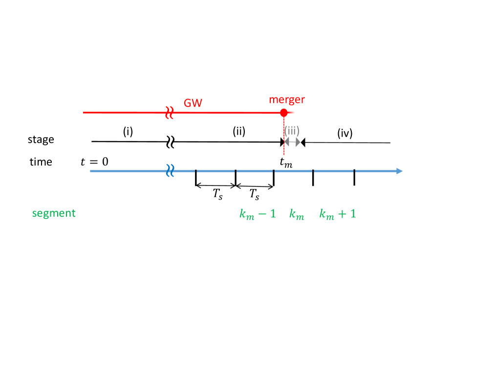
Figure 1: Schematic diagram for observation of a GW signal from a merging WDB. We set the time origin $t=0$ at the beginning of LISA’s operation and put the merger time by $t=t_{\rm m}$. We divide the time sequence into the four stages (i)-(iv) with the duration $\Delta t_{\rm p}$ and $\Delta t_{\rm t}$ respectively for (ii) and (iii). For the identification of the merger time $t_{\rm m}$, we introduce the time segmentation with an appropriately selected duration $T_{\rm s}$. The merger time $t_{\rm m}$ is in the segment $k=k_{\rm m}$.

For coherent signal integration with the matched filtering analysis, the phase of the target GW should be accurately characterized by a limited number of fitting parameters (e.g., the polynomial expansion with the derivative coefficients $f^{(n)}$ at some epoch). Unlike a well separated WDBs, even in the time region of nearly monochromatic GW emission, a WDB close to the merger might have complicated GW phase modulations which should be handled with a short-term phenomenological phase modeling. As a precaution for such a potential difficulty, we conservatively divide the time region of nearly monochromatic emission into two stages (i) and (ii). We put $\Delta t_{\rm p}$ as the total duration of the late monochromatic stage (ii). Sorting out the temporal sequence, around the merger time $t_{\rm m}$, we now have the following four stages.

(i) Early monochromatic stage at $t<t_{\rm m}-\Delta t_{\rm p}$. The binary emits nearly monochromatic GW at the frequency $\sim f_{\rm m}$ with the amplitude $\sim h_{\rm m}$. Its intrinsic GW phase can be coherently described by a simple expression.

(ii) Late monochromatic stage at $t_{\rm m}-\Delta t_{\rm p}<t<t_{\rm m}$. The binary continues to emit nearly monochromatic wave at $\sim f_{\rm m}$ and $\sim h_{\rm m}$. We need phenomenological phase model with a short integration period.

(iii) Transition stage at $t_{\rm m}<t<t_{\rm m}+\Delta t_{\rm t}$. The disruption of the donor proceeds rapidly and the emitted GW no longer has regular monochromatic pattern, due to hydrodymanical effects.

(iv) Post-merger stage at $t_{\rm m}+\Delta t_{\rm t}<t$. Virtually no GW is emitted, as the merged system settles down to a nearly stationary and axisymmetric configuration.

Here we can practically assume $\Delta t_{\rm p}\gg\Delta t_{\rm t}$ (otherwise we do no need to introduce the late stage (ii)). In contrast to the transition duration $\Delta t_{\rm t}$ deduced from existing numerical simulations, the magnitude of $\Delta t_{\rm p}$ is currently unclear. We need to accurately follow the longer-term dynamical evolution at high mass resolution. Numerical approach would be highly demanding, and analytical study might be more advantageous. Observational studies on known short-period WDBs might be also useful (see e.g. Strohmayer 2021; Munday et al. 2023 for RX J0806.3+1527). Below, we leave the duration $\Delta t_{\rm p}$ as a free parameter, just assuming $\Delta t_{\rm p}\ll 1$yr. We should also comment that the boundary between (i) and (ii) is not mathematically distinct. It is rather a practical one and depends on the complexity of the phase modeling allowed for the stage (i).

3 Observation with LISA

Next we discuss matched filtering analysis with LISA. We set the origin of the time coordinate $t=0$ at the beginning of LISA’s operation. Given its planned operation period 4-10 yr, we below set $t_{\rm m}=2$yr as a conservative average. For the purpose of concise illustration, we are assumed to make two kinds of data analysis: the long-term search and the segmented short-term search.

The purpose of the long-term search is to confidently detect a WDB and determine its basic parameters, using the data at the early monochromatic stage (i). This search would be similar to the signal analysis for a standard (non-merging) WDB. Using the results of the long-term search, we subsequently perform the segmented short-term searches for identifying the disappearance of its nearly monochromatic GW at the merger. In reality, we can chronologically mix these two searches.

3.1 The Long-Term Search

Throughout the early monochromatic stage (i), the GW signal would be coherently searched with manageable numerical costs. The total signal-to-noise ratio $\rho$ can be estimate as

$$\rho=\frac{h_{\rm m}\sqrt{T}}{S_{n}(f_{\rm m})^{1/2}}$$ (8)

for the integration time $T$. Here, for simplicity, we ignore the angular dependence of the GW strain (Cutler, 1998). It is straightforward to include it in our analysis below.

As presented in Table 1 for $T=t_{\rm m}=2$yr, the expected signal-to-noise ratio in the stage (i) is $\rho=O(100)$ and much larger than those for typical Galactic LISA sources existing at lower frequencies. For the base model A (up to the end of the stage (ii)), the signal-to-noise ratio squared $\rho^{2}$ increases unity in every $\sim 180$ wave cycles, corresponding to $\sim$0.1 day ($\sim 430$ cycles for B and $\sim 50$ cycles for C). Therefore, even though the catastrophic stage (iii) is interesting, this stage is likely to have a negligible contribution to the signal-to-noise ratio, given its rotation cycles of $\lesssim 10$ (Dan et al., 2011). For our signal analysis scheme, we can omit the stage (iii) and effectively regard that the nearly monochromatic stage (ii) is directly followed by the quiet stage (iv) at the merger time $t_{\rm m}$.

Using the high quality signal in the stage (i), we can securely confirm the existence of the binary. We can also estimate its nearly monochromatic frequency $f_{\rm m}$ and other basic parameters including the amplitude $h_{\rm m}$. For instance, the sky position of the binary can be determined with the aid of the Doppler modulation (Cutler, 1998). For $T\gtrsim 2$yr, we can apply an asymptotic scaling relation for the area of the error ellipsoid (Takahashi & Seto, 2002)

$$\Delta\Omega\sim 0.01\left(\frac{\rho}{85}\right)^{-2}\left(\frac{f}{\rm 20.8mHz}\right)^{-2}{\rm deg^{2}}.$$ (9)

The area becomes $\rm\sim 0.06deg^{2}$ for the model B. The high sky localization would be beneficial for associated EM observations.

3.2 Segmented Short-Term Search

Let us suppose that we have already done the long-term search for a WDB, in the middle of its early monochromatic stage (i). Now, we divide the upcoming data streams into segments of a duration $T_{\rm s}$ as shown in Fig. 1. We assign the label $k$ and put $\rho_{k}$ for the corresponding signal-to-noise ratio obtained after the short-term coherent matched filtering. The total number of the segments increases, as LISA’s operation period becomes longer.

Our immediate goal is to observationally determine the specific segment $k_{m}$ which contains the merger time $t_{\rm m}$ (see Fig. 1). To this end, we appropriately set the threshold $\rho_{\rm th}$ and the duration $T_{\rm s}$, so that we can reliably have $\rho_{k}\geq\rho_{\rm th}$ for earlier segments $k<k_{m}$ and $\rho_{k}<\rho_{\rm th}$ for later segments $k>k_{m}$, due to the existence of the nearly monochromatic wave before the merger time $t_{\rm m}$.

Here, in terms of statistical tests, we want to suppress the false dismissal rate $P_{\rm FDR}$ for $k<k_{m}$ and the false alarm rate $P_{\rm FAR}$ for $k>k_{m}$, both caused by the flukes of the noise realizations (Buonanno, Chen, & Vallisneri, 2003). We should notice that, for the target WDB, presupposing the high-quality information from the already analyzed data (in the stage (i)), the implication of these two rates are somewhat different from the blind short-lived binary search with the current LVK network (The LIGO Scientific Collaboration et al., 2021).

For a segment at $k>k_{m}$, assuming Gaussian noise, the false alarm rate is estimated to be

$$P_{\rm FAR}=\frac{\cal N}{\sqrt{2\pi}}\int_{\rho_{\rm th}}^{\infty}{\exp\left[-\frac{\rho^{2}}{2}\right]}d\rho=\frac{\cal N}{2}{{\rm erfc}\left[\frac{\rho_{\rm th}}{2^{1/2}}\right]}$$ (10)

with the effective number of the templates $\cal N$ and the complementary error function $\rm erfc(\cdot)$. Note that the function ${{\rm erfc}\left[{\rho_{\rm th}}/{2^{1/2}}\right]}/2$ depends very strongly on $\rho_{\rm th}$ and we have $10^{-2},10^{-3},10^{-5}$ and $10^{-7}$ respectively for $\rho_{\rm th}=2.3$, 3.1, 4.3 and 5.2. The effective number of templates $\cal N$ depends on the possible phase models (and the integration time $T_{\rm s}$). After all, in our pilot study, we shifted the uncertainty of the stage (ii) to that of the template number $\cal N$. In the actual data analysis, we can use the information of the earlier segments, for empirically extending the phase models. At present, on the basis of the strong dependence on $\rho_{\rm th}$, we adopt the reference value $\rho_{\rm th}=5$ for $P_{\rm FAR}=10^{-2}$. If we actually have $\Delta t_{\rm p}\ll T_{\rm s}$, our setting $\rho_{\rm th}=5$ will result in a very conservative choice.

Next we discuss the false dismissal rate for an earlier segment $k<k_{m}$. Using the results (e.g., $h_{\rm m}$ and $f_{\rm m}$) from the preceding long-term search, we can estimate the expectation value

$$\left\langle\rho_{k}\right\rangle=\frac{h_{\rm m}\sqrt{T_{\rm s}}}{S_{n}(f_{\rm m})^{1/2}}$$ (11)

as a function of the segment duration $T_{\rm s}$. Then, by adjusting the duration $T_{\rm s}$, we can evaluate the false dismissal rate as

$$P_{\rm FDR} = \frac{1}{\sqrt{2\pi}}\int^{\rho_{\rm th}}_{-\infty}{\exp\left[-\frac{(\rho-\left\langle\rho_{k}\right\rangle)^{2}}{2}\right]}d\rho$$ (12)

$$= \frac{1}{2}{{\rm erfc}\left[\frac{\left\langle\rho_{k}\right\rangle-\rho_{\rm th}}{2^{1/2}}\right]}.$$ (13)

For $P_{\rm FDR}\sim 10^{-2}$, we have

$$\left\langle\rho_{k}\right\rangle\simeq\rho_{\rm th}+2.5=7.5.$$ (14)

We can inversely obtain the segment duration $T_{\rm s}$ by

$$T_{\rm s}=\left\langle\rho_{k}\right\rangle^{2}S_{n}(f_{\rm m})h_{\rm m}^{-2}.$$ (15)

In Table 1, we present the numerical results for $T_{\rm s}$, together with the corresponding rotation cycles $f_{\rm m}\cdot T_{\rm s}$. For the base model, we have $T_{\rm s}=5.7$ day and 10000 cycles.

From the arguments so far, we can easily see that, for the critical segement $k=k_{m}$, we have $\rho_{k}\geq\rho_{\rm th}$ or $\rho_{k}<\rho_{\rm th}$, depending on the location of the merger time $t_{\rm m}$ in the segment.

3.3 Estimation of the Merger Time

Next we discuss the estimation of the merger time $t_{\rm m}$ from the growing list $\{\rho_{k}\}$ obtained after repeating the short-term matched filtering. To proceed in a dualistic manner, we map the signal-to-noise ratios $\rho_{k}$ by

$$F_{k}\equiv\theta(\rho_{k}-\rho_{\rm th})$$ (16)

with the step function $\theta(\cdot)$. We will have $F_{k}=1$ for $k<k_{m}$ and $F_{k}=0$ for $k>k_{m}$ ($F_{k}=1$ or 0 for $k=k_{m}$). Then, the list $\{F_{k}\}$ should have the following form

$$\{F_{k}\}=\{1,1\cdots,1,\underline{1,0},0,0,0,\cdots\}.$$ (17)

The merger time $t_{\rm m}$ should contained in the two specific segments marked with the underline. Therefore, the half width $\delta t_{\rm m}$ of the estimation error becomes

$$\delta t_{\rm m}=2^{-1}(2T_{\rm s})=T_{\rm s}.$$ (18)

So far, we have fix the segmentation. By relaxing this setting, we can further analyze the two candidate segments above. More specifically, we put a slidable segment characterized by the starting time $x$ (keeping the duration at $T_{\rm s}$) as

$$k(x)\equiv[x,x+T_{\rm s}].$$ (19)

We define the associated signal-to-noise ratio $\rho(x)$ for this segment. We can identify the maximum value $x=x_{\max}$ which satisfies $F[\rho{(x)}]=1$. Similarly, we read the minimum value $x=x_{\min}$ for $F([\rho{(x)}]=0$ with $x_{\max}\leq x_{\min}$. Here, the inequality can be caused by an intricate pattern of the function $F[\rho{(x)}]$ due the noise. The merger time $t_{\rm m}$ should be contained simultaneously in the two segments $k(x_{\max})$ and $k(x_{\min})$. Taking their overlapped part, we can estimate the merger time with a half width of

$$\delta t_{\rm m}\leq T_{\rm s}/2,$$ (20)

corresponding to $\lesssim 3$ days for our base model.

The estimated magnitude $\delta t_{\rm m}$ is much larger than the transition period $\Delta t_{\rm t}$ around the merger. Therefore, as mentioned earlier, we practically do not need to too rigidly define the merger time $t_{\rm m}$ (e.g., before or after the transition stage (iii)).

4 Discussion

So far, we have discussed matched filtering analysis for a merging Galactic WDB with LISA. Here, from a broader perspective, we mention related topics and potential extension of this work.

4.1 GW data analysis

We have assumed $\Delta t_{\rm p}\ll$1yr, for the duration $\Delta t_{\rm p}$ of the late monochromatic stage (ii). Currently, it is not straightforward to solidly estimate the duration $\Delta t_{\rm p}$ introduced for precautionary purpose. As already commented, we can rather evaluate the potential phase evolution, by empirically using the existing earlier data of the binary (smoothly from the stage (i)). Similarly, the number of effective templates $\cal N$ will be estimated reasonably well at the actual data analysis in the stage (ii).

In a very pessimistic scenario with $\Delta t_{\rm p}\gtrsim$2yr, we might not have the simple stage (i), which has played a key role in our data analysis procedure. A semi-coherent search could be a powerful option, as currently applied to unknown pulsar search with the LVK network (Abbott et al., 2022). GW from a WDB could be observed at much higher signal-to-noise ratio with much smaller rotation cycles. Therefore, depending on the phase irregularity, our task could be much easier than the unknown pulsar search with the LVK network.

At estimating the merger time $t_{\rm m}$, we have used a matched filtering analysis just for checking the disappearance of a nearly monochromatic GW signal (without decoding its detailed structure). In reality, the wave phase might be relatively simple with a precursor signature for the forthcoming merger. Then, we might predict the merger time $t_{\rm m}$ by carefully performing matched filtering analysis. If this is the case, our estimation $\delta t_{\rm m}$ should be regarded as a very conservative bound. On another front, while we have introduced the mapping (16) for our simple dualistic argument, the original function $\rho(x)$ can be directly analyzed for the estimation of the merger time $t_{\rm m}$.

Note that, if the operation period of LISA is longer than $\sim 1$yr, the Galactic confusion noise is negligible in the frequency regime $f\gtrsim 5$mHz (Robson, Cornish, & Liu, 2019; Littenberg et al., 2020). Therefore, for a donor mass $m_{1}\gtrsim 0.3M_{\odot}$ shown in Table 1, the interference with other binary signals is likely to be insignificant. However, we have $f_{\rm m}\sim 5$mHz, for a smaller donor mass $m_{2}\sim 0.1M_{\odot}$. For such a binary, we might need to securely suppress the interference effects at the LISA multi source-analysis. Consequently, the required segment duration $T_{\rm s}$ could be longer than that estimated from Eq. (11).

We can try other efficient methods (e.g., the chi-square analysis), particularly in the context of the low latency analysis. The non-Gaussianity of detector noises might be also worth studying.

4.2 Other Space Interferometers

Here we briefly comment on space interferometers other than LISA. Since a WDB mainly emits a nearly monochromatic GW, our results scale simply with the instrumental noise spectrum $S_{n}(f)$, as shown in Eqs. (8) and (15).

Around 20mHz, the sensitivities of Taiji (Ruan et al., 2018) and TianQin (Luo et al., 2016) are quite similar and approximately two times better than that of LISA. Meanwhile, at $\sim$20mHz, B-DECIGO (Kawamura et al., 2021) is designed to have a sensitivity similar to LISA, but its optimal band is in the higher frequency regime around 100mHz (Isoyama, Nakano, & Nakamura, 2018). B-DECIGO and its follow-on mission DECIGO (Seto, Kawamura, & Nakamura, 2001) might thereby enable us to detect extra-Galactic merging WDBs with total masses higher than the Chandrasekhar mass (possibly relevant for SNIa) (Maselli, Marassi, & Branchesi, 2020; Kinugawa et al., 2022).

4.3 EM Observation

When we try to identify an EM counterpart to a WDB, its binary parameters (e.g., those related to orbital phase, sky location and inclination) will be critically useful. Once identified, we can continue to frequently observe the binary with EM telescopes, even after the operation period of LISA. Moreover, we might monitor the transitional merger stage (iii) with the telescopes. Such an observation will provide us with valuable information on white dwarfs and, possibly, its explosion mechanism. The archived data much before LISA’s launch might be also useful for studying a WDB in a long time span (Digman & Hirata, 2022).

5 summary

The merger rate of Galactic WDBs is roughly estimated to be $\rm\sim 0.02yr^{-1}$. In this paper, we discuss identification of a merger event in the data streams of LISA. Until very close its final merger, a typical WDB will emit nearly monochromatic GW around 20mHz. After a short transition period, it will virtually stop emitting GW. LISA has potential to detect its nearly monochromatic GW with a signal-to-noise ratio of $O(10^{2})$ and determine its sky location within $\sim 0.01$-$0.1{\rm deg^{2}}$. By repeatedly checking the disappearance of its nearly monochromatic GW, we could robustly estimate its merger time with accuracy of $\sim 3$-10 days.

References

- Abbott et al. (2022) Abbott R., Abe H., Acernese F., Ackley K., Adhikari N., Adhikari R. X., Adkins V. K., et al., 2022, PhRvD, 106, 102008. doi:10.1103/PhysRevD.106.102008
- Amaro-Seoane et al. (2022) Amaro-Seoane P., Andrews J., Arca Sedda M., Askar A., Balasov R., Bartos I., Bavera S. S., et al., 2022, arXiv, arXiv:2203.06016. doi:10.48550/arXiv.2203.06016
- Benz et al. (1990) Benz W., Bowers R. L., Cameron A. G. W., Press W. H., 1990, ApJ, 348, 647. doi:10.1086/168273
- Breivik et al. (2018) Breivik K., Kremer K., Bueno M., Larson S. L., Coughlin S., Kalogera V., 2018, ApJL, 854, L1. doi:10.3847/2041-8213/aaaa23
- Buonanno, Chen, & Vallisneri (2003) Buonanno A., Chen Y., Vallisneri M., 2003, PhRvD, 67, 024016. doi:10.1103/PhysRevD.67.024016
- Cutler (1998) Cutler C., 1998, PhRvD, 57, 7089. doi:10.1103/PhysRevD.57.7089
- Dan et al. (2011) Dan M., Rosswog S., Guillochon J., Ramirez-Ruiz E., 2011, ApJ, 737, 89. doi:10.1088/0004-637X/737/2/89
- Dan et al. (2014) Dan M., Rosswog S., Brüggen M., Podsiadlowski P., 2014, MNRAS, 438, 14. doi:10.1093/mnras/stt1766
- Digman & Hirata (2022) Digman M. C., Hirata C. M., 2022, arXiv, arXiv:2212.14887. doi:10.48550/arXiv.2212.14887
- D’Souza et al. (2006) D’Souza M. C. R., Motl P. M., Tohline J. E., Frank J., 2006, ApJ, 643, 381. doi:10.1086/500384
- Hils, Bender, & Webbink (1990) Hils D., Bender P. L., Webbink R. F., 1990, ApJ, 360, 75. doi:10.1086/169098
- Isoyama, Nakano, & Nakamura (2018) Isoyama S., Nakano H., Nakamura T., 2018, PTEP, 2018, 073E01. doi:10.1093/ptep/pty078
- Kawamura et al. (2021) Kawamura S., Ando M., Seto N., Sato S., Musha M., Kawano I., Yokoyama J., et al., 2021, PTEP, 2021, 05A105. doi:10.1093/ptep/ptab019
- Kinugawa et al. (2022) Kinugawa T., Takeda H., Tanikawa A., Yamaguchi H., 2022, ApJ, 938, 52. doi:10.3847/1538-4357/ac9135
- Korol et al. (2017) Korol V., Rossi E. M., Groot P. J., Nelemans G., Toonen S., Brown A. G. A., 2017, MNRAS, 470, 1894. doi:10.1093/mnras/stx1285
- Lamberts et al. (2019) Lamberts A., Blunt S., Littenberg T. B., Garrison-Kimmel S., Kupfer T., Sanderson R. E., 2019, MNRAS, 490, 5888. doi:10.1093/mnras/stz2834
- Littenberg et al. (2020) Littenberg T. B., Cornish N. J., Lackeos K., Robson T., 2020, PhRvD, 101, 123021. doi:10.1103/PhysRevD.101.123021
- Lorén-Aguilar, Isern, & García-Berro (2009) Lorén-Aguilar P., Isern J., García-Berro E., 2009, A&A, 500, 1193. doi:10.1051/0004-6361/200811060
- Luo et al. (2016) Luo J., Chen L.-S., Duan H.-Z., Gong Y.-G., Hu S., Ji J., Liu Q., et al., 2016, CQGra, 33, 035010. doi:10.1088/0264-9381/33/3/035010
- Maoz, Hallakoun, & Badenes (2018) Maoz D., Hallakoun N., Badenes C., 2018, MNRAS, 476, 2584. doi:10.1093/mnras/sty339
- Marsh, Nelemans, & Steeghs (2004) Marsh T. R., Nelemans G., Steeghs D., 2004, MNRAS, 350, 113. doi:10.1111/j.1365-2966.2004.07564.x
- Maselli, Marassi, & Branchesi (2020) Maselli A., Marassi S., Branchesi M., 2020, A&A, 635, A120. doi:10.1051/0004-6361/201936848
- Moran-Fraile et al. (2023) Moran-Fraile J., Schneider F. R. N., Roepke F. K., Ohlmann S. T., Pakmor R., Soultanis T., Bauswein A., 2023, arXiv, arXiv:2303.05519
- Munday et al. (2023) Munday J., Marsh T. R., Hollands M., Pelisoli I., Steeghs D., Hakala P., Breedt E., et al., 2023, MNRAS, 518, 5123. doi:10.1093/mnras/stac3385
- Nelemans et al. (2001) Nelemans G., Yungelson L. R., Portegies Zwart S. F., Verbunt F., 2001, A&A, 365, 491. doi:10.1051/0004-6361:20000147
- Nissanke et al. (2012) Nissanke S., Vallisneri M., Nelemans G., Prince T. A., 2012, ApJ, 758, 131. doi:10.1088/0004-637X/758/2/131
- Paczyński (1967) Paczyński B., 1967, AcA, 17, 287
- Pakmor et al. (2013) Pakmor R., Kromer M., Taubenberger S., Springel V., 2013, ApJL, 770, L8. doi:10.1088/2041-8205/770/1/L8
- Rasio & Shapiro (1992) Rasio F. A., Shapiro S. L., 1992, ApJ, 401, 226. doi:10.1086/172055
- Raskin et al. (2012) Raskin C., Scannapieco E., Fryer C., Rockefeller G., Timmes F. X., 2012, ApJ, 746, 62. doi:10.1088/0004-637X/746/1/62
- Robson, Cornish, & Liu (2019) Robson T., Cornish N. J., Liu C., 2019, CQGra, 36, 105011. doi:10.1088/1361-6382/ab1101
- Ruan et al. (2018) Ruan W.-H., Guo Z.-K., Cai R.-G., Zhang Y.-Z., 2018, arXiv, arXiv:1807.09495. doi:10.48550/arXiv.1807.09495
- Ruiter et al. (2010) Ruiter A. J., Belczynski K., Benacquista M., Larson S. L., Williams G., 2010, ApJ, 717, 1006. doi:10.1088/0004-637X/717/2/1006
- Schwab (2018) Schwab J., 2018, MNRAS, 476, 5303. doi:10.1093/mnras/sty586
- Seto, Kawamura, & Nakamura (2001) Seto N., Kawamura S., Nakamura T., 2001, PhRvL, 87, 221103. doi:10.1103/PhysRevLett.87.221103
- Seto (2022) Seto N., 2022, PhRvL, 128, 041101. doi:10.1103/PhysRevLett.128.041101
- Shen et al. (2012) Shen K. J., Bildsten L., Kasen D., Quataert E., 2012, ApJ, 748, 35. doi:10.1088/0004-637X/748/1/35
- Strohmayer (2021) Strohmayer T. E., 2021, ApJL, 912, L8. doi:10.3847/2041-8213/abf3cc
- Takahashi & Seto (2002) Takahashi R., Seto N., 2002, ApJ, 575, 1030. doi:10.1086/341483
- The LIGO Scientific Collaboration et al. (2021) The LIGO Scientific Collaboration, the Virgo Collaboration, the KAGRA Collaboration, Abbott R., Abbott T. D., Acernese F., Ackley K., et al., 2021, arXiv, arXiv:2111.03606. doi:10.48550/arXiv.2111.03606
- Verbunt & Rappaport (1988) Verbunt F., Rappaport S., 1988, ApJ, 332, 193. doi:10.1086/166645
- Wolz et al. (2021) Wolz A., Yagi K., Anderson N., Taylor A. J., 2021, MNRAS, 500, L52. doi:10.1093/mnrasl/slaa183
- Yoshida (2021) Yoshida S., 2021, ApJ, 906, 29. doi:10.3847/1538-4357/abc7bd