Algorithmic Censoring in Dynamic Learning Systems

Abstract.

Dynamic learning systems subject to selective labeling exhibit censoring, i.e. persistent negative predictions assigned to one or more subgroups of points. In applications like consumer finance, this results in groups of applicants that are persistently denied and thus never enter into the training data. In this work, we formalize censoring, demonstrate how it can arise, and highlight difficulties in detection. We consider safeguards against censoring – recourse and randomized-exploration – both of which ensure we collect labels for points that would otherwise go unobserved. The resulting techniques allow examples from censored groups to enter into the training data and correct the model. Our results highlight the otherwise unmeasured harms of censoring and demonstrate the effectiveness of mitigation strategies across a range of data generating processes.

1. Introduction

Machine learning (ML) models are often used in dynamic learning systems that combine training, prediction, and data collection. In applications like consumer finance, hiring, data-driven discovery, and disease screening, these systems are subject to selective labeling, meaning we only collect labels for instances that are assigned a positive prediction (Lakkaraju et al., 2017).

Dynamic learning systems that are subject to selective labeling exhibit censoring – i.e., they may fail to assign a positive prediction to one or more subgroups of points . Such subgroups are repeatedly assigned negative predictions despite model updates, thus never entering into the training data. This makes it difficult for the system to correct mistakes or adapt to new patterns.

Censoring is a blind spot of dynamic learning systems – one that is not necessarily good or bad. Consider a model for loan approval that censors a sub-population of applicants (e.g., individuals without credit history). Censoring may be justified for an applicant who would have ultimately defaulted on their loan. Conversely, it may be unjustified if the applicant would have ultimately repaid their loan. The underlying issue is in the ambiguity: one cannot distinguish between these two populations because we will never approve the applicant and thus never observe their true label.

The potential harms of censoring are magnified through feedback loops. In dynamic learning systems, predictions influence current decisions and data collected to train future models. Consider a consumer who lacks credit history applies for a loan. Their credit report is input into a model that outputs a probability of repayment and makes a subsequent decision. For this consumer, the lack of credit history results in a low predicted probability and subsequent rejection. This results in two costs for the consumer: 1) they do not receive the loan, 2) they are unable to build credit history to strengthen their loan application. This puts them at risk for becoming a “credit invisible”, i.e. an applicant who is locked out of the credit system due to their inability demonstrate creditworthiness (Kozodoi et al., 2021). In the United States, this “catch 22” affects approximately 26 million consumers (Blattner and Nelson, 2021; Brevoort et al., 2015; noc, 2022). This is just one example of an individual perpetually denied consideration of a social system through algorithms alone. Censoring can lead to issues across various machine learning applications:

• Hiring: Companies use models to screen resumes and make decisions about which candidates to interview  (Das, 2021). These systems exhibit censoring as certain subgroups of applicants will never be interviewed nor hired, therefore never entering into the training data. The resulting models may only hire employees similar to those historically hired. In practice, this can hurt both businesses and individuals by excluding qualified applicants (Li et al., 2020; Raghavan et al., 2020; Engler, 2021b, a).

• Disease Screening: Medical practitioners may train disease detection models on pre-existing datasets (Sengupta and Shrestha, 2019; Zhao et al., 2022). In dermatology, models are used to predict which lesions should be subject to further inspection (Soenksen et al., 2021). A model that systematically misclassifies a subset of melanoma-prone lesions may put the corresponding individuals at a higher risk of cancer and/or death. Beyond a consistently incorrect negative prediction, they may also never entering the training dataset to correct the model.

• Data-Driven Discovery: In materials science, drug discovery, and chemistry, scientists obtain recommendations for promising experiments based on models trained on small labelled datasets (Raccuglia et al., 2016; Bergen et al., 2019; Pollice et al., 2021). In drug discovery, for example, scientists may fit a model to predict if a given chemical compound can act as a antibiotic. Compounds that receive higher predicted probabilities are then slated for a confirmatory experiment. In such settings, models may consistently miss a promising subset of molecules that are dissimilar to historical positive examples. In turn, censored molecules will never be assigned high probabilities and never tested in confirmatory experiments. In this case, censoring could lead to less efficient discovery processes or missed discoveries.

Contributions

The main contributions of this work include:

1. We define and formalize censoring, describe why it is difficult to detect, and how it may lead to harms.

2. We demonstrate how censoring can arise and catalog four such mechanisms: sample selection bias, heterogeneity in data quality, operational changes, and distributional shifts.

3. We describe general-purpose strategies to safeguard against censoring, characterizing their costs and benefits for different stakeholders.

4. We present a comprehensive study to benchmark general-purpose approaches to resolve and safeguard against censoring. Our study evaluates each technique on dynamic settings that vary in terms of the complexity of the data distributions, propensity for strategic manipulation, and the ability to target the censored group. We conclude that recourse is best in settings with causal features, as it provides a directed exploratory approach to censoring-group validation. We propose a combination of recourse and randomization as a solution for unknown causal settings.

Related Work

We explore the implications of selective labeling and censoring in dynamic learning systems (DLSs). Prior work studies the implications of selective labeling in a static setting (Lakkaraju et al., 2017; Blum and Stangl, 2019; De-Arteaga et al., 2018; Coston et al., 2021). We consider this effect in dynamic environments (Lum and Isaac, 2016; Liu et al., 2018; Kallus and Zhou, 2018; Gu and Oelke, 2019; D’Amour et al., 2020; Hu and Chen, 2018; Jiang et al., 2021) that involve multiple rounds of data collection, training, and prediction (Ensign et al., 2018; De-Arteaga et al., 2018; Hashimoto et al., 2018; Jiang et al., 2021). Our work shows that these systems may exhibit feedback loops that lead to persistent denial of individuals. We demonstrate the difficulty in detecting this effect and identify its impact to model-owners as well as individuals. Prior work explores leveraging unlabelled data an intervention at model training (Lee and Liu, 2003; Elkan and Noto, 2008; Hu et al., 2021; Rateike et al., 2022; Aka et al., 2021), whereas we examine post-training safeguards: randomization and recourse.

The traditional approach to resolve censoring in the reinforcement learning literature is to explore (Ensign et al., 2017; Kilbertus et al., 2020; Chen et al., 2020; Kulkarni and Neth, 2020; Brown et al., 2020; Dai, 2020; Krauth et al., 2020; Mansour et al., 2021; Erdélyi et al., 2021; Simchowitz and Slivkins, 2021; Immorlica et al., 2018; Wei, 2020; Chandak et al., 2020) – i.e., to build dynamic learning systems that collect data that would inform future decisions. Exploration may be ill-suited for certain applications that exhibit censoring because they involve randomization. In effect, a randomized policy may be unethical in consumer-facing applications like hiring, lending, and disease-screening, as individuals who are approved at random may be subject to harms such as job insecurity, poor credit, and unnecessary medical tests (Goldstein et al., 2018; Royall, 1991; Baunach, 1980; Colli et al., 2014). More broadly, these techniques may also be ill-suited because exploratory policies are only guaranteed to optimize population measures of long-term utility or regret. These measures may not be responsive to censoring because they are too broad to capture the impact of a small group of individuals.

Recourse, i.e. when providing individuals with actionable changes to obtain a desired predicted outcome, is another solution to safeguard against censoring (Ustun et al., 2019; Venkatasubramanian and Alfano, 2020; Karimi et al., 2020b, a; von Kügelgen et al., 2020). Work in strategic classification shows that recourse can promote gaming when provided on non-causal features, resulting in a change in the predicted outcome without a corresponding change in the true outcome. Causal recourse actions – i.e., actions that change both the predicted outcome and true outcome – however, may lead to improvement (Bechavod et al., 2020, 2021; Shavit et al., 2020; Chen et al., 2019; Milli et al., 2019; Levanon and Rosenfeld, 2021). Our work complements this by exploring additional failure modes, such as that due to model shift (see e.g., Upadhyay et al., 2021; Rawal et al., 2020), retraining (Ross et al., 2021), and by considering recourse with explicit guarantees, or a combination of recourse and exploration.

The most relevant work to ours is that of Kilbertus et al. (2020), which studies a similar setting through the lens of reinforcement learning. Their approach casts models as “approval policies" in a finite-horizon Markov decision process and seeks to find a model that maximizes utility for a model-owner (e.g., a lender) under a group fairness constraint. Although their work does not study censoring, shows that deterministic policies will achieve sub-optimal regret due to insufficient exploration. This is one of the potential consequences of censoring, as models may assign incorrect predictions to individuals who would have positively impacted utility.

2. Framework

In this section, we formalize the notion of censoring in dynamic learning systems.

2.1. Preliminaries

We consider a sequential decision-making process over $t=1,\ldots,T$ with $T\geq 2$ periods. We initialize the process with $n^{1}$ initial training examples denoted $D^{1}:=(\bm{x}_{i},y_{i})_{1}^{n^{1}}$. Each example consists of feature vector $\bm{x}_{i}=[x_{i,1},\ldots,x_{i,d}]\in\mathbb{R}^{d}$ and label ${y_{i}\in\{-1,1\}}$ where $y=1$ denotes a target class (e.g., repaid loan within 2 years). We denote the true probability of the target outcome as $p^{t}:\mathcal{X}\to\textnormal{Pr}\left(Y=1~{}|~{}X=\bm{x}_{i}\right)$ and the predicted probability from the model as $\hat{p}^{t}:\mathcal{X}\to\textnormal{Pr}\left(Y=1~{}|~{}X=\bm{x}_{i}\right)$. Each period applies the following three steps:

1. Fit: We use the dataset $D^{t}$ to fit a probabilistic classifier $\hat{h}^{t}{}:\mathcal{X}\to[0,1]$ via standard empirical risk minimization:

   $$\hat{p}^{t}{}\in\operatorname*{argmin}_{h\in\mathcal{H}}\hat{R}(h;D^{t})$$

   where $\hat{R}(h;D^{t})$ denotes the empirical risk (e.g., negative log-likelihood) and $\mathcal{H}$ denotes the model class. We assume that model owners convert the probability predictions from $\hat{h}^{t}{}$ into predictions by a threshold $\rho\in[0,1]$ so that $\hat{y}_{\rho}(\bm{x}_{i})=1$ if and only if $\hat{p}(\bm{x}_{i})>\rho]$.

2. Predict: We use the model $\hat{y}^{t}$ to assign predictions to all incoming examples in period $t$: $n_{\textnormal{eval}}^{t}:=n_{\textnormal{new}}^{t}+n_{\textnormal{ret}}^{t}$. We use $n_{\textrm{new}}^{t}$ to denote new points that are sampled i.i.d. from an unknown data distribution, and $n_{\textnormal{ret}}^{t}$ to denote instances assigned negative predictions in previous periods $t^{\prime}<t$.

3. Collect: We append labelled examples to the training dataset. Given that the system exhibits selective labeling, we observe $\bm{x}_{i}$ for all $n_{\textnormal{eval}}^{t}$ points at prediction time, and observe labels for instances assigned the prediction $\hat{y}^{t}(\bm{x}_{i})=1$. We add $n^{t+1}$ examples to the training data, where

   $$n^{t+1}:=\left|D^{t+1}\right|=\sum_{k=1}^{t}\sum_{i=1}^{n_{\textnormal{eval}}^{k}}\mathbbm{1}[\hat{y}^{k}(\bm{x}_{i})=1]=n^{t}+\sum_{i=1}^{n_{\textnormal{eval}}^{t}}\mathbbm{1}[\hat{y}^{t}(\bm{x}_{i})=1]$$

   . We note that the observed label is probabilistic and therefore not all observed data has the desired outcome.

2.2. Censoring

Definition 0 (Censoring).

A dynamic learning system censors instances with features $\bm{x}$ if it fails to observe a label $y(\bm{x})$ over the entirety of deployment lifetime without intervention. In other words, all models predict ${\hat{y}^{t}(\bm{x})=-1}$ for all future periods $t\in[t,\ldots,T]$. We denote $c^{t}(\bm{x})=-1$ if the system censors instances with features $\bm{x}$ from periods $t$ onwards and $c^{t}(\bm{x})=1$ if the system does not censor instances with features $\bm{x}$ from period $t$ onwards.

Censoring characterizes a blind spot of DLSs, one that does not necessitate a failure in performance. Consider a lending system that censors applicant $i$. By definition, this means that the system will assign negative predictions to any instance with features $\bm{x}_{i}$ in perpetuity. This phenomenon may be optimal if the predicted and true label are in agreement subject to some tolerance $\tau$: $\textnormal{Pr}\left(\hat{y}(\bm{x}_{i})=y(\bm{x}_{i})\right)>\tau$. Conversely, the system performs suboptimally if the predictions are not in agreement – i.e., $\textnormal{Pr}\left(\hat{y}(\bm{x}_{i})=y(\bm{x}_{i})\right)<\tau$. In a system exhibiting censoring, the system’s optimality is unverified and unknown, as we never observe the outcome label for the censored group.

Given this blind-spot, censoring causes problems in DLS when: (1) the system presumes that the label for the point is negative even though it may be positive, and (2) the system does not validate this assumption nor correct this mistake. This behavior is particularly dangerous in various settings: i.e., those with high label noise, where the model was initialized on a small training set, or where the relationship between $\bm{x}_{i}$ and $y_{i}$ drifts over time. We examine such settings in Section 3, where we induce censoring on immutable covariate $z=1$ where $c_{i}=z_{i}=1$ for systems with censoring with no intervention. We use $z=1$ to calculate metrics on the initially censored group to measure the unobserved harms and efficacy of resolving censoring when safeguards are deployed.

3. Mechanisms that Induce Censoring

In this section, we describe four mechanisms that lead to censoring: sample selection bias, heterogeneity in data quality, operational changes, and distributional shifts, although these are not exhaustive.

Preliminaries

For each mechanism, we provide an empirical example and report the observed and true AUC to demonstrate difficulty in detection. The true AUC is calculated on an unbiased sample from the underlying data distribution while the observed AUC is calculated on the training data collected over time.

For clarity, the group of censored points have covariate $z=1$ censored points using the censoring indicator $z_{i}:=\hat{y}^{t}(\bm{x}_{i})=-1$ for $t\in\{t^{\prime},\ldots,T\}$. Note that ${z_{i}=1\Leftrightarrow z_{i}^{\prime}=1}$ for any points $i$ and $i^{\prime}$ such that ${\bm{x}_{i}=\bm{x}_{i^{\prime}}}$ – i.e., when a system has censored a point, it censors all other points with the same features. In practice, censoring may affect groups defined by multiple subsets of features, further exacerbating difficulty of detection. For example, a lending system could censor applicants below the age of 35 without a credit card – i.e., ${\bm{x}\in x_{i,j}\land x_{i,j^{\prime}}}$ where ${x_{i,j}=1[{\textit{age}}\leq 35]}$ and ${x_{i,j^{\prime}}=1[{\textit{has\_credit\_card}}={\textit{FALSE}}]}$. Each mechanism can cause censoring in deployed systems, be it individually or simultaneously.

Outcome	Population $z\in\{-1,1\}$	Censored Group $z=1$
$y\in\{-1,1\}$
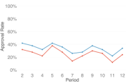
$y=1$

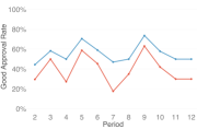
Figure 1. Unrepresentative training data leads to censoring. We train models by sampling from causal data generating process in Table 3. We show a system initialized with a baseline unbiased sample (blue) and an unrepresentative sample where we have no data for individuals with features $z_{i}=1$ and outcome $y_{i}=1$ (red). As shown, the model trained on the unrepresentative sample censors all $z_{i}=1$ points. We demonstrate that censoring is difficult to detect via standard performance metrics – the training AUC at the last period is similar: 0.811 (unrepresentative training data) and 0.795 (representative training data), while the true AUC, is much worse for unrepresentative training data (0.660) than representative training data (0.756).

Sample Selection Bias

Censoring can arise when a model is trained on data unrepresentative of the deployment population. This occurs when model-owners use readily available data, such as in already deployed products. This can be favorable to model-owners due to the convenience and accessibility of readily available data and the prohibitive costs of collecting new data (time, money, personnel). These costs can be particularly discouraging when attempting to estimate the requisite sample size for unknown or low occurrence subgroups. For instance, historical roots of lending in the US include institutionalised “redlining”, disfavoring applicants from neighborhoods that were “within such a low price or rent range as to attract an undesirable element,” which often meant near predominantly Black neighborhoods (Rice and Swesnik, 2013; Greer, 2012; Alliance, 2012). Black people and people of color more generally were deemed high risk, refused loans, and never entered into the training data, leaving their true repayment status unrealized. This is used to perform data-driven risk prediction today (Dobbie et al., 2021; Bhutta et al., 2022).

We demonstrate how this leads to censoring in a system with an initial model trained on an unrepresentative training dataset in Figure 1. Here, $D^{1}$ is biased as it is missing $y=1$, $z=1$ points, leading it to mistakenly predict all $z=1$ points to be negative. As a result, the approval rate for all $z=1$ points is $0$ for the entirety of the system’s lifetime, despite making up 15% of the population. This pattern persists unresolved over multiple rounds of data collection, retraining, and deployment and is not reflected in the AUC.

Heterogeneity in Data Quality

Censoring can also arise from heterogeneity in the data distribution. For labels, noise can arise from intrinsic ambiguity due to human annotation (Khanal and Kanan, 2021; Yan et al., 2014; Veit et al., 2017; Chen et al., 2017; Wei et al., 2021). For features, noise can arise from intrinsic difficulty in measurement (Zhang et al., 2021). In lending in the US, for example, models use features that are measured with higher rates of noise for historically marginalized groups (e.g., credit history Blattner and Nelson, 2021; Kelley and Ovchinnikov, 2021). These individuals are referred to as “credit invisibles”(Brevoort et al., 2015) and are assigned uncertain predictions. Such predictions leads to perpetual denial and censoring: such denied individuals cannot produce labeled data and therefore increase their credit history due to the original prediction.

We demonstrate how censoring can arise via heterogeneity in label noise in Table 1. We consider a system where examples have some probability of exhibiting the desired true outcome and compare two systems: one with label noise and one without. In the system without label noise, a Bayes optimal classifier correctly approves all $\bm{x}=1$ points. However, the system with label noise incorrectly assigns a negative prediction to all points with $z=1,\bm{x}=1$. Although we only show a single round of decision-making, this behavior will be repeated at each round of deployment.

				No Label Noise			With Label Noise
$n$	$x$	$z$	$\textnormal{Pr}\left(y=1\right)$	Observed Label ($y$)		Model Prediction	$p_{\textrm{flip}}{}(x,z,y)$		Observed Label ($y$)		Model Prediction
				-1	1		-1	1	-1	1	($\hat{y}$)
100	0	-1	0	100	0	0	0	0	100	0	-1
100	0	1	0.4	60	40	0	0	0.4	76	24	-1
100	1	-1	1	0	100	1	0	0	0	100	1
100	1	1	0.7	30	70	1	0	0.4	58	42	-1

Table 1. Example showing how an initial model trained with noisy labels and a probabilistic true outcome can lead to censoring. We train models on dataset with $n=400$ examples from groups $z\in\{-1,1\}$. We assume that the observed labels in the training data $y$ may differ from the predicted value due to noise. As shown, a Bayes optimal model incorrectly predicts $\hat{y}(x=1,z=1)=-1$, therefore censoring such points. The observed AUC (only for positive predicted points) for the systems with no label noise and label noise are the same (0.500), while the true AUC is 0.826 and 0.738 respectively.

Outcome	Population $z\in\{0,1\}$	Censored Group $z=1$
$y\in\{-1,1\}$
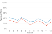
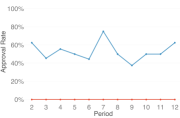
$y=1$

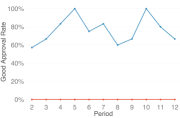
Figure 2. Operational changes can induce censoring. We consider the causal setup in Table 3. We show a system initialized on an baseline sample (blue) and a system initialized on a sample acquired from a one time adjustment to the $b$ in the first period (red). The operational change system exhibits censoring on all $z=1$ points despite similar overall approval rates. In this system, the observed AUC is 0.790 with operational changes and 0.774 in the system without operational changes. However, the true AUC is 0.638 and 0.756, respectively.

Operational Changes

Censoring can also arise from operational changes – i.e. when a model-owner adjusts the approval criteria of a pretrained model. For instance, in lending, if a model-owner implements a more conservative approval policy due to economic hardship or external regulation (ECO, 2021; Kumar et al., 2022; Press, [n. d.]; FHA, [n. d.]; Akinwumi et al., 2022; US_, 2022; UK_, [n. d.]), they may increase the requisite predicted repayment probability for approval. As a result, some subgroups may be excluded by the initial model, resulting in downstream propagation of these biases. Although such subgroups may have limited representation in the initial training data, the bias incurred from a single round of deployment may perpetuate the subgroup denial bias for all subsequent models even through retraining, censoring such groups in perpetuity.

We demonstrate how operational changes can lead to censoring in Fig. 2. Here, we consider a stylized example where we make a one-time adjustment on the initial model $b$. We observe that after the initial $b$ change, all models denies $Z=1$ individuals for all rounds of deployment.

Outcome	Population $z\in\{-1,1\}$	Censored Group $z=1$
$y\in\{-1,1\}$
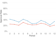
$y=1$

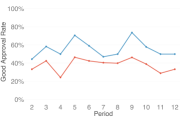
Figure 3. Distributional shifts can induce censoring. We consider the causal setup specified in Table 3. We show a system initialized with an $x_{1}$ feature shift for $z=1$ in initial training data – specifically, before: $x_{1}\sim\textrm{Normal}(0,1)$, after $x_{1}\sim\textrm{Normal}(-5,1)$. As shown, feature shift induces censoring of all $z=1$, being persistently denied for all periods. Again, this is difficult to detect as the observed AUC is 0.787 in for the system with feature shift and 0.756 for the system without, even though the true AUC is actually much worse for the system with feature shift (0.614) than the one without (0.756).

Distributional Shifts

Censoring can arise due to distributional shifts – i.e., changes in the relationship between the features and/or labels. Feature shift can occur in many ways, we will enumerate three.

First, the underlying feature distribution can change between training and deployment (i.e., covariate shift Quiñonero-Candela et al., 2009). Such changes could result from broader shifts in the population. In lending, for instance, the distribution of applicants that are home-owners may change as a result of the true underlying data distribution changing, such as if homes became less affordable.This can also be a result of a shift in the observed data distribution, such as if home ownership status stops being collected, but is still included in the model. These can result in incorrect predicted risk and subsequent persistent denial of qualified applicants.

Second, feature shift can occur for a subgroup of the population  (Shimodaira, 2000). In lending, the distribution of applicants that are homeowners may change due to required features becoming opt-in instead. For applicants that might have previously had verified home-ownership, they may choose not to disclose such information, resulting in incorrect predicted risk and subsequent persistent denial of credit-worthy applicants.

Third, features present in training that are hard to measure in deployment can cause feature shift. In lending, suppose legislation making home-ownership verification a expensive and lengthy process is passed, making it generally avoided by lenders. This may again result in incorrect predicted risk and subsequent denial towards qualified applicants. We demonstrate feature shift induced censoring for the $z=1$ population in Figure 3.

4. Mitigation

Having seen some of the ways in which censoring may arise, we consider some general-purpose safeguards: randomization and recourse. We provide definitions, scope, technical challenges, and limitations. We demonstrate that these safeguards resolve censoring through empirical experiments in Section 5.

4.1. Exploration

One of the most studied approaches to exploration is randomized or stochastic decision rules. Randomized exploration allows for a proportion of negative-predicted points to enter into the training dataset, allowing model-owners to validate the model for censored subgroups. If a model assigns incorrect predictions to a subgroup, these examples can inform future models.

Setup

We describe methods for randomized exploration: uniform, which randomly selects instances for points assigned negative prediction; and inverse propensity score weighting (IPW), which weighs the probability of selection inversely proportional to the assigned probability $\hat{p}{}$. This assigns a greater exploration likelihood for points unlikely to be observed through model shift from retraining alone.

Formally, uniform randomization approves some $\alpha$-proportion of points assigned negative predictions to collect labels. Points assigned negative predictions are approved with equal probability:

$$\textnormal{Pr}\left(\bm{x}_{i}\in D^{t+1}~{}|~{}\hat{y}_{t}(\bm{x}_{i})=-1\right)=\alpha.$$

Fig. 4 shows an example of how randomization can resolve censoring for a true positive subgroup. Without randomization, the $Z=1$ subgroup are perpetually assigned negative predictions throughout the system lifetime. Randomization approves a subset of points assigned $\hat{y}_{t}=-1$, providing an opportunity for the model to learn that the $Z=1$ group is $\mathcal{Y}=1$. This helps protect against censoring when model-owners lack knowledge of exactly which consumer segment is being censored.

Outcome	Population $z\in\{-1,1\}$	Censored Group $z=1$
$y\in\{-1,1\}$
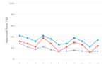
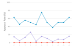
$y=1$

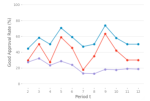
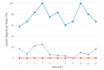
Figure 4. Toy example where randomization solves censoring. We compare results of three systems under the causal setup: a system without censoring (blue), a system with censoring (red), and a system with censoring that randomly approves some denied applicants (purple). The randomization allows censored applicants to enter into the training data and correct the model.

While this approach is individually fair (i.e., across experimental units), it may require many rounds of randomization to observe examples from a censored group, especially when the group consitutes a small part of the overall population. Therefore we also consider randomization with inverse propensity score weighting (IPW), which assigns a greater approval likelihood to points with lower predicted probabilities $\hat{h}(\bm{x}_{i})$, as such points are the least likely to be assigned a positive prediction from noise alone or model drift due to retraining. Formally:

$$\textnormal{Pr}\left(\bm{x}_{i}\in D^{t+1}~{}|~{}\hat{y}_{t}(\bm{x}_{i})=-1\right)=\frac{1}{\hat{p}^{t}(\bm{x}_{i})}\sum_{\begin{subarray}{c}\bm{x}_{j}\in D^{t+1},\\ \hat{y}_{t}(\bm{x}_{i})=-1\end{subarray}}\hat{p}^{t}{}(\bm{x}_{j})$$

Scope

Randomization may not be suitable for all applications due to ethical concerns. For instance, in lending, random exploration may approve loans for individuals likely to default. While individuals have agency over whether to accept the loan, being offered a loan might express confidence that individuals can repay it. This might make individuals more likely to accept the loan, resulting in negative consequences such as crippling their credit scores and preventing future loan qualification (Havard, 2005; Squires, 2017). IPW, in particular, may exacerbate these harms, as individuals with low-confidence predictions are more likely to be approved and thus will disproportionately bear the burdens of exploration.

Technical Challenges

Randomization may be difficult to guarantee. In lending, for example, applicants may submit applications to various banks in addition to reducing their likelihood of getting a loan (in the case of IPW) to increase their chances of approval. In addition, randomization may also make models difficult to explain. In applications where consumers are entitled to information on why they were denied, stochastic classifiers are harder to justify to any one individual who was and was not randomly explored upon (Kagan, 2020).

Limitations

Though randomization can resolve censoring, it can be costly, particularly when false negatives are a small proportion of all negative predictions. For instance, if the censored group is only 1% of the denied population and uniform randomization is employed at $\alpha=0.01$. Then in expectation, the system will have to employ randomization for 100 periods before they collect a single data point from the censored group. However, the collection of this point alone will not resolve censoring, as the system will have to gather enough examples of those from the censored group to predict $\hat{y}=1$. So the system will likely have to employ randomization for much more than 100 periods before correcting on such a censored group. This is extremely time and resource costly for both model-owners and points.

Randomization also raises equity concerns in regards to differential approval rates for “identical” individuals – i.e. those with the same features. The legality of such methods are context dependent. In lending, this may be perceived as a fair classifier, but in recidivism prediction, this may violate individuals’ rights to equal treatment in the 14th amendment of the US Constitution (fdi, 2021; Baunach, 1980; Colli et al., 2014).

4.2. Recourse

An alternative safeguard against censoring is recourse, i.e., providing individualized feature changes that result in the desired prediction (Ustun et al., 2019). Recourse resolves some of the ethical challenges posed by randomization because it gives experimental units agency over their predictions and provides a common set of rules. When applied to causal features, it can lead to improvement of the prediction pool, as actions increase the predicted and true probability of the outcome, making this exploratory method lower-risk. We demonstrate how recourse can mitigate censoring in Figure 5.

Setup

Formally, recourse provides points with actions, i.e. feature changes, that when added to the original features, result in the desired predicted outcome. Actions that are real-world feasible and actionable can be solved via the following optimization:

$$\begin{split}\min\quad&\textrm{cost}(\bm{a}_{i};\bm{x}_{i})\\ \textnormal{s.t.}\quad&\hat{y}(\bm{x}_{i}+\bm{a}_{i})=1\\ &\bm{a}_{i}\in A(\bm{x}_{i})\end{split}$$

Here, we solve for a set of features changes $\bm{a}_{i}$ such that when they are added to a point $i$’s original features $\bm{x}_{i}$, result in the desired predicted outcome. Actions $\bm{a}$ are restricted by real-world constraints such as directionality (i.e., can only increase education), mutability (i.e., savings balance), and feasibility/realism (i.e., a savings balance increase of $500 not $100,000).

Outcome	Population $z\in\{-1,1\}$	Censored Group $z=1$
$y\in\{-1,1\}$
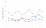
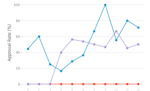
$y=1$

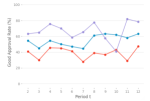
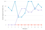
Figure 5. Toy example where recourse resolves censoring. We compare the results of three systems under the causal setup: a system without censoring (blue), a system with censoring (red), and a system with censoring that provides recourse to denied applicants (purple). The recourse allows censored applicants to enter into the training data and correct the model.

Scope

Providing recourse may be unethical in settings where you cannot guarantee its availability for the entire population. This may arise from recourse infeasibility, i.e. there are not available feature changes that result in the desired predicted outcome, stemming from immutable features or feature domain limitations. Recourse may additionally be unethical to deploy on non-causal features, as feature changes may be ineffective and unnecessarily costly.

Technical Challenges

Recourse is not a stand-alone solution. It does not provide guarantees and requires cooperation between model-owners and users. Specifically, recourse provides actions calculated under the current model, not robust to model or distributional changes(Upadhyay et al., 2021). In addition, while causal recourse actions have the potential to provide improvement(Miller et al., 2020), true causal model is rarely known, meaning non-causal recourse actions have the potential to enable gaming. As a result, we also explore recourse with guarantees in Section 5.

Limitations

Cost of recourse estimation is an open area of research. As such, costs may be difficult to estimate and/or heterogeneously distributed across the population. In addition, equivalent actions in the eyes of the model may vary in the cost across individuals. This raises additional questions on how many equivalent actions should be provided.

5. Experiments

In this section, we evaluate the two proposed strategies to safeguard against censoring. For clarity, we use language specific to the lending application, referring to ‘points that receive a negative prediction’ as ‘denied applicants’, and ‘points that received a negative prediction and are subject to a new prediction in the next period’ as ‘reapplicants’. However, we emphasize that censoring is salient to many dynamic learning system domains.

5.1. Setup

We compare seven mitigation strategies against two baselines: None and NoCensoring. These baselines reflect systems where censoring does and does not occur, respectively. All remaining mitigation strategies are employed with systems initializes with censoring induced via sample selection bias defined in Section 3. We further detail each mitigation strategy in Table 2.

Name		Label Collection Policy	Description
Censoring		$\hat{y}_{\rho}(\bm{x}_{i})=1$	This system suffers from censoring and demonstrates the difficulty of detection of censoring. This system quantifies the potential harms censoring that would otherwise be immeasurable in real-world system and serves as a worst-case scenario baseline to evaluate the impact of other policies.
NoCensoring		$\hat{y}_{\rho}(\bm{x}_{i})=1$	This system is not subject to censoring and represents the best-case scenario. This system serves as a baseline of optimal performance to evaluate the impact of other policies.
Random		$\hat{y}_{\rho}(\bm{x}_{i})=1\cup\alpha|\hat{y}_{\rho}(\bm{x}_{i})=-1|$	We use a semi-logistic policy to collect labels from two groups: 1) those with the predicted probability of $Y=1$ above the operating threshold of 0.5, and 2) a random sample of 1% of points below the operating threshold that would otherwise be unobserved.
IPW		$\hat{y}_{\rho}(\bm{x}_{i})=1\cup\alpha|\hat{y}_{\rho}(\bm{x}_{i})=-1|$	We use a semi-logistic policy to collect labels from two groups: 1) those with the predicted probability of $Y=1$ above the operating threshold of 0.5, and 2) through inverse probability weighting, 1% of otherwise unobserved true outcomes. This means we prioritize exploring on points farther from the decision boundary, as such points are very less likely to be observed through retraining alone.
Rec		$\hat{y}^{t}_{\rho}(\bm{x}_{i})=1$	We observe labels for points in two groups: 1) those above the operating threshold, and 2) those that have made feature changes according to previously deployed models that are above the operating threshold. We provide no guarantees of feature change robustness to future model retraining, meaning some points may undergo multiple feature changes before their true outcome is observed.
Rec_Guarantee		$\hat{y}^{t}_{\rho}(\bm{x}_{i})=1\cup\hat{y}^{t-1}_{\rho}(\bm{x}_{i})=-1$	We observe the labels for points from the current period with predicted probabilities above the operating threshold and unobserved points from the previous period after having undergone recourse generated feature changes. Since all points enact recourse actions before the following period, we only need to provide guarantees that account for one period (see Section 6). This allows a special track for evaluation that ensures that such points are guaranteed approval.

Table 2. Overview of baselines and mitigation strategies. We consider systems where we train a standard logistic regression model with $\ell_{2}$ regularization to the training dataset aggregated over time. We assign positive predictions when the predicted probability exceeds 50%. Strategies that employ randomization use an exploration rate of $\alpha=0.01$. $t$ is used to denote the current period.

Data Generating Processes

We evaluate each strategy on eight data-generating processes (DGPs) shown in Table 3. Each DGP is specified by a directional acyclic graph (DAG), which defines the joint distribution of features and outcomes and allows us to evaluate the effect of interventions on the outcome $Y$. We consider different DGPs that vary in causality and complexity to study the effects of censoring and evaluate the effectiveness of mitigation strategies.

Simulation

We initialize the system with a classifier $\hat{y}^{1}$ that exhibits censoring by training on a sample selection biased data. We define the censored group as all $z=1$ individuals and drop all positive examples – i.e., $\{i~{}|~{}(z_{i},y_{i})=(1,1)\}$. We simulate each system for $T=12$ periods. At period $t$, we fit a logistic regression model with $\ell_{2}$ regularization $\hat{y}^{t}$ using $D^{t}$. We then use $\hat{y}^{t}$ to assign predictions to $n_{\textrm{new}}^{t}=100$ new applicants, and $n_{\textnormal{ret}}^{t}$ reapplicants from earlier periods. The system approves applicants assigned a predicted probability greater than $\rho=0.5$.

In systems where we provide recourse (Rec, Rec_Guarantee), we generate recourse actions to all denied applicants using the software of (Ustun et al., 2019). We assume all applicants execute these actions before reapplying the following period. In systems with randomization(Random, IPW), we approve $\alpha=0.01$ denied applicants. We collect examples for $(\bm{x}_{i},y_{i})$ for all approved applicants and add them to the training data for the following period $D^{t+1}$.

Evaluation

We evaluate each mitigation strategy on a variety of metrics defined in Table 4. These metrics are designed to capture the interests of model-owners and decision subjects. The metrics demonstrate the challenges in detection – i.e., by reporting the metrics for the observed and true (unbiased) populations, as well as for the censored and non-censored group ($z=1$). We run each simulation ten times and report summary statistics across replicates.

5.2. Results

We summarize our results in Fig. 6. First, we demonstrate that censoring is not resolved through retraining alone and that it is difficult to detect. Second, we compare trade-offs among safeguards, varying across feature causality. Finally, we provide high-level recommendations across all settings, in particular for unknown causal settings.

		Baselines		Exploration		Recourse		Combined
Data Generating Process	Metrics	Censoring	NoCensoring	Random	IPW	Rec	Guarantee	Rec + Random	Guarantee + IPW	Rec + IPW
causal $y=x_{1}+x_{2}+z-0.5$ $\hat{y}=x_{1}+x_{2}+z+b$ $\textnormal{Pr}\left(Z=1\right)=15\%$	Observed AUC True AUC Gain/Loss % Approved % Approved | $Z=1$ $\mathbb{E}$[Reapplications] Net Improvement	0.795 0.671 1.0/1.0 24.2% 0.0% - -	0.779 0.777 1.3/1.0 33.8% 58.6% - -	0.783 0.738 1.2/1.2 18.6% 14.6% 3.59 -	0.79 0.744 1.2/1.2 17.1% 21.3% 3.31 -	0.767 0.727 1.6/1.3 49.5% 41.6% 1.21 21.7%	0.766 0.733 1.4/1.2 40.2% 38.2% 1.00 26.0%	0.767 0.738 1.6/1.3 54.0% 53.0% 1.17 22.1%	0.767 0.736 1.4/1.2 40.0% 38.0% 1.00 25.8%	0.767 0.738 1.6/1.3 49.5% 48.7% 1.24 21.1%
causal_blind $y=x_{1}+x_{2}$ $\hat{y}=x_{1}+x_{2}+z+b$ $\textnormal{Pr}\left(Z=1\right)=15\%$	Observed AUC True AUC Gain/Loss % Approved % Approved | $Z=1$ $\mathbb{E}$[Reapplications] Net Improvement	0.817 0.729 1.0/1.0 29.6% 0.2% - -	0.789 0.782 1.2/1.0 35.2% 33.5% - -	0.806 0.757 1.1/1.2 20.3% 12.3% 3.56 -	0.816 0.733 1.0/1.0 9.6% 1.2% 3.36 -	0.789 0.767 1.5/1.3 51.9% 47.3% 1.21 23.1%	0.787 0.763 1.3/1.2 40% 43.2% 1.00 28.0%	0.789 0.766 1.5/1.3 55.9% 51.2% 1.17 24.1%	0.787 0.764 1.2/1.2 39.7% 42.8% 1.00 27.8%	0.789 0.763 1.5/1.3 53.2% 48.6% 1.17 23.8%
causal_linked $y=x_{1}+x_{2}+z-0.5$ $\hat{y}=x_{1}+x_{2}+z+b$ $\textnormal{Pr}\left(Z=1\right)=15\%$	Observed AUC True AUC Gain/Loss % Approved % Approved | $Z=1$ $\mathbb{E}$[Reapplications] Net Improvement	0.837 0.766 1.0/1.0 30.8% 2.7% - -	0.826 0.836 1.3/1.0 39.1% 56.7% - -	0.834 0.809 1.1/1.2 21.3% 16.6% 3.58 -	0.841 0.811 1.1/1.2 21.1% 22.6% 3.36 -	0.811 0.780 1.2/1.2 44.8% 19.0% 1.28 17.9%	0.807 0.771 1.0/1.1 28.6% 11.1% 1.00 22.7%	0.812 0.801 1.3/1.2 49.6% 37.4% 1.27 18.2%	0.807 0.772 1.0/1.1 28.5% 11.3% 1.00 22.7%	0.813 0.778 1.2/1.2 44.7% 20.5% 1.29 17.6%
causal_equal $y=x_{1}+x_{2}+z-1.5$ $\hat{y}=x_{1}+x_{2}+z+b$ $\textnormal{Pr}\left(Z=1\right)=15\%$	Observed AUC True AUC Gain/Loss % Approved % Approved | $Z=1$ $\mathbb{E}$[Reapplications] Net Improvement	0.792 0.707 1.0/1.0 28.3% 0.0% - -	0.764 0.774 1.2/1.0 33.9% 33.7% - -	0.783 0.742 1.1/1.2 20% 12.1% 3.63 -	0.791 0.712 1.0/1.0 9.1% 1.2% 3.56 -	0.761 0.726 1.4/1.3 48.7% 21.3% 1.21 21.4%	0.756 0.726 1.2/1.2 37.1% 20.5% 1.00 26.1%	0.768 0.753 1.5/1.3 54.7% 43.3% 1.17 24.0%	0.76 0.73 1.2/1.2 37.4% 24.7% 1.00 26.3%	0.763 0.733 1.5/1.3 50.3% 32.7% 1.19 22.2%
mixed_proxy $y=x_{1}+x_{2}+z-0.5$ $\hat{y}=x_{1}+x_{2}^{non}+z+b$ $\textnormal{Pr}\left(Z=1\right)=15\%$	Observed AUC True AUC Gain/Loss % Approved % Approved | $Z=1$ $\mathbb{E}$[Reapplications] Net Improvement	0.799 0.679 1.0/1.0 25.5% 0.3% - -	0.782 0.776 1.3/1.0 35.1% 59.8% - -	0.786 0.739 1.2/1.2 19.1% 14.9% 440 -	0.793 0.746 1.2/1.2 17.8% 22.9% 3.27 -	0.767 0.705 1.5/1.3 43.9% 35.5% 1.40 12.4%	0.762 0.697 1.3/1.3 39.8% 32.5% 1.00 17.8%	0.77 0.728 1.5/1.3 49% 50.6% 1.36 12.9%	0.762 0.703 1.3/1.3 40% 34.8% 1.00 17.9%	0.768 0.707 1.5/1.3 44.9% 42.9% 1.44 12.3%
mixed_downstream $y=x_{1}+z-0.5$ $\hat{y}=x_{1}+x_{2}^{\textnormal{non}}+z+b$ $\textnormal{Pr}\left(Z=1\right)=15\%$	Observed AUC True AUC Gain/Loss % Approved % Approved | $Z=1$ $\mathbb{E}$[Reapplications] Net Improvement	0.813 0.697 1.0/1.0 25.9% 0.1% - -	0.799 0.802 1.3/1.0 35.5% 63.1% - -	0.802 0.764 1.2/1.2 19.5% 16% 3.54 -	0.808 0.771 1.1/1.2 18.3% 24.1% 3.24 -	0.783 0.747 1.5/1.3 46% 44.5% 1.38 10.6%	0.775 0.747 1.3/1.3 41.1% 43.2% 1.00 15.2%	0.783 0.757 1.5/1.3 49.5% 54.3% 1.39 10.4%	0.775 0.752 1.2/1.3 40.9% 42.7% 1.00 15.0%	0.785 0.747 1.5/1.3 46.6% 45.8% 1.39 10.6%
gaming $y=x_{1}+z-0.5$ $\hat{y}=x_{1}^{\textnormal{non}}+x_{2}^{\textnormal{non}}+z+b$ $\textnormal{Pr}\left(Z=1\right)=15\%$	Observed AUC True AUC Gain/Loss % Approved % Approved | $Z=1$ $\mathbb{E}$[Reapplications] Net Improvement	0.805 0.697 1.0/1.0 25.2% 0.4% - -	0.794 0.799 1.3/1.0 35.1% 65.5% - -	0.796 0.763 1.2/1.2 19.3% 17.1% 3.54 -	0.803 0.769 1.2/1.2 18.2% 24.5% 3.35 -	0.761 0.707 1.3/1.3 39.1% 28.4% 1.68 3.2%	0.741 0.703 1.2/1.3 40.7% 34.2% 1.00 5.0%	0.76 0.732 1.4/1.4 45% 45.3%  1.53 3.5%	0.741 0.711 1.2/1.3 41.2% 39.1% 1.00 4.7%	0.759 0.716 1.4/1.4 41.1% 36.8% 1.60 3.1%
german $y=0.3(-l-d+i+s)$ $\hat{y}=g+a+e+l$ $+d+i+s+b$	Observed AUC True AUC Gain/Loss % Approved (all) % Approved | $G=1$ $\mathbb{E}$[Reapplications] % Net Improvement	0.74 0.572 1.0/1.0 16.8% 1.4% - -	0.704 0.678 2.0/1.1 44.3% 48.7% - -	0.989 0.986 7.0/6.7 28.1% 27.1% 3.56 -	0.988 0.986 1.9/1.0 23.6% 22.6% 2.71 -	0.726 0.563 1.2/1.1 21.8% 8.4% 1.47 -32.0%	0.722 0.572 1.2/1.4 37.7% 36.6% 1.00 -45.0%	0.711 0.577 1.2/1.2 27.3% 15.7% 1.40 -33.1%	0.725 0.571 1.2/1.4 38.2% 37.2% 1.00 -44.0%	0.724 0.561 1.2/1.2 22.3% 9.0% 1.49 -31.1%

Figure 6. Overview of censoring and mitigation strategies across data generating processes. We highlight results referenced in our remarks: Censoring Does Not Resolve Itself Without Intervention, On the Difficulties of Detection, All Mitigation Methods Recover from Censoring, Recourse Works Best in Causal Settings, IPW for Greater Censored Group Uncertainty, and Combination Methods: A Solution For Unknown Causal Settings. These phenomena arise across DGPs. We use $b$ to specify the intercept.

Censoring Does Not Resolve Itself Without Intervention

Across all DGPs, using the no safeguard strategy (Censoring) collects labels for $0\%$ of censored group points, compared to the optimal approval rate of $>58\%$ in NoCensoring. This is also reflected in the net gain across all setups with NoCensoring, particularly when compared to the baseline None. In addition, all systems exhibit censoring across all periods, indicating dynamic learning systems do not recover from retraining alone.

On the Difficulties of Detection

Censoring is difficult to detect using performance metrics alone. Across all DGPs with no safeguards (Censoring), the observed AUC (only considering the points assigned positive predictions) is greater than the unbiased sample (true AUC). For instance, in the mixed_proxy DGP, the observed AUC is 0.799, while the true AUC is 0.679. Since model-owners only observe the labels for positively predicted points, they do not observe their performance on those assigned negative predictions. This inflates the AUC, providing model-owners a false estimate of performance. In addition, we provide uncertainty metrics: miscalibration area, sharpness score, and root mean squared adversarial group calibration error in Appendix D, observing little differences between observed and true, further emphasizing the difficulty in detecting censoring.

5.2.1. Trade-offs Between Mitigation Strategies

Mitigation strategies impose different costs and trade-offs across all stakeholders. These also vary across strategy, degree of guarantee/robustness provided, cost of errors, feature causality, and ease of feature observability. Below we make high-level recommendations for navigating such trade-offs.

All Mitigation Methods Recover from Censoring

Across all DGPs, all randomization, recourse, and combination methods recover from censoring. All strategies result in the approval of a non-zero approval rate for the censored group. For instance, Rec approves 41.6% on average while Censoring approves 0% of $z=1$ applicants in the causal DGP. Each mitigation strategy provides an avenue for otherwise perpetually unobserved points to enter into the dataset. Once the censored group points are collected into the training dataset, the model is more likely to recover from censoring, even when undetected. This demonstrates how these safeguards serve as a self-correction mechanism, functioning without precursory knowledge of what defines the censored points.

Recourse Works Best in Causal Settings

In settings with causal model features, recourse is less costly than randomization. For model-owners, the approval rate for $z=1$ points is greater in all recourse treatments than in randomization, indicating a faster rate of recovery. For instance, in causal Rec, we observe 41.6% compared to 21.3% approved in IPW. In addition, the net improvement of recourse actions is greatest in models with more causal features: 21.7% less likely to result in a negative outcome in Rec compared to 12.4% in mixed_proxy. This is consistent across all causal setups (i.e., causal, causal_blind, causal_linked, causal_equal). Recourse allows for focused, directed exploration for otherwise unobserved points. When recourse can lead to improvement, applicants can change their features to increase both the predicted and actual likelihood of the positive outcome.

For censored points, the expected number of reapplications is lower in causal settings: 1.21 vs 3.59 reapplications in Rec and Random in causal, meaning that any costs incurred from being reevaluated is smaller in recourse as compared with randomization. In addition, when no recourse guarantees are provided (Rec_Guarantee), the proportion of invalid recourse actions is lower in causal settings: 0.203 versus 0.359 in causal and mixed_proxy, respectively. This suggests that in settings where the model features are known to be causal on the outcome, recourse is less costly than randomization. In recourse settings, Guarantee also decreases the expected number of reapplications. While this is beneficial to censored points, it also incurs additional costs to model-owners.

Failure Modes of Recourse: Infeasibility

In fully causal settings, recourse may still fail when actions are too costly or outside of the feature range. This is called infeasible recourse. This can arise when a model requires a feature change greater than that allowed for the feature to produce a positive prediction. These limitations can be specified by the training data or by real-world directional or bound limitations. We demonstrate how recourse fails to mitigate censoring in Fig. 7 due to feature range limitations. Recourse infeasibility is important to consider as it may provide model-owners the illusion of a safeguard without providing the actual benefit.

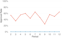
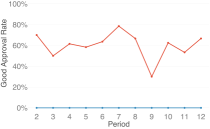
Figure 7. Recourse cannot solve censoring if it is infeasible. Here, we consider a systems suffering from censoring under the Causal setup. The leftmost plot shows the model coefficients in a setting where recourse is feasible, i.e. $X_{1}\in[-2,1.5]$ allows for recourse actions large enough to overcome the incorrect initial negative coefficient on $z$. This allows $z=1$ applicants to enter into the training dataset and correct the model, as shown by the $z$ coefficient increasing over iterations. In the second plot we show the model coefficients a setting where recourse is infeasible, i.e. $X_{1}\in[-2,1]$. Denied applicants cannot take recourse actions on $x_{1}$ large enough to be approved. Thus, the system continues suffering from censoring and the coefficient for $z$ stays negative. The third and fourth plots show the approval rates for the $z=1$ and the $z=1,y=1$ subgroups (the latter indicating the % approved of those wrongfully censored) in of the feasible recourse system (red) and the infeasible recourse system (blue). We observe the approval rate for the censored group is $0\%$ in the infeasible setting and $>0$ for the feasible setting.

IPW for Greater Censored Group Uncertainty

Across all settings IPW has a higher censored group approval rate, such as 14.9% in Random, compared to 22.9% in IPW for mixed_proxy. This is due to the nature of how censoring is induced, i.e. by removing all $z=1,y=1$ examples from the training set. The resulting initial model then had a low $\hat{y}$ for such examples, meaning IPW could more effectively ensure that such examples were included in future training sets, rather than uniform selection across all negatively predicted samples. If instead the censored group was closer to the initial decision boundary (closer to the predicted probability of $\hat{p}=1)$ cutoff), then Random would have been more effective. Thus, the efficacy of randomized exploration employed may still vary across the nature of the censoring. Settings with greater vulnerability to high inaccuracy censoring (larger disparities in error of predicted probabilities) may achieve more success with IPW. Random, however, may be a better catch-all alternative.

Combination Methods: A Solution For Unknown Causal Settings

In settings with uncertainty about causality and recourse feasibility, model-owners may opt for combination methods, such as Rec+Random. In both causal and non-causal settings, Rec+Random has the highest % Approved for the $z=1$ group. In the causal setup, the system approves 53.0% of censored group applications compared to 0% in Censoring and 58.6% in NoCensoring. mixed_proxy approves 50.6%, compared to 0.4% and 65.5% of censored group applicants in Censoring and NoCensoring. Gaming, approves 45.3% in Rec+Random, compared to 0.4% and 65.5% in None and NoCensoring. Rec+Random also consistently has a lower expected number of reapplications than Random, IPW, and Rec. In causal_blind, Rec+Random has 1.27 expected reapplications, compared to 3.58 in Random, 3.36 in IPW, and 1.28 in Rec. This phenomena still holds in the gaming setup: with 1.53 reapplications in Rec+Random, 3.54 in Random, 3.35 in IPW, and 1.68 in Rec.

6. Concluding Remarks

In this work, we formalize the censoring phenomenon, demonstrate several causes, highlight the difficulty in detection, and propose two families of safeguards for mitigation. We study the prevalence censoring under data generating processes that characterize salient applications – those that identify potential effects that inflict harm and affect the effectiveness of mitigation. We define and compute metrics that quantify the harms to stakeholders often not considered in DLSs, such as decision-subjects and their respective cumulative harms. Our results show that recourse works best in causal settings, becoming more costly in mixed or non-causal settings. We propose combination methods for unknown causal settings, given that both randomization and recourse may be ethical in such settings.

Our experiments manually induce censoring. This enables us to quantify the harms and costs of censoring that go undetected and unmeasured in deployed systems. In reality, censored groups can be defined across any subset of features, making detection all the more difficult. In particular, in settings where we want to ensure equal access to the associated benefits of the positive predicted outcome, we emphasize the importance of deploying such mitigation methods. Censoring represents a potential harm in which individuals are denied consideration of a social system solely through algorithms alone. These harms should not only be considered, but prioritized.

Limitations

We discuss key considerations, design decisions, and simplifying assumptions made in this work.

In our experiments, we assume that the time between periods is fixed and consistent (e.g., 2 years as is the norm in lending). In general, however, this is not always clearly defined. In drug discovery, for example, the next period may only begin after we have collected sufficient samples to re-train our model. In effect, such models are still subject to selective labeling, allowing for censoring to arise. However, variations in period length will impact the rate of recovery from censoring and the potential to resolve changes through recourse or other feature changes.

We recommend carefully considering the degree of model trust or uncertainty before deploying recourse, as it has varying degrees of efficacy. Recourse is particularly complex to operationalize as causal relationships are rarely known, may be heterogeneous across the population, or change with time. Additional barriers to feature selection and may include difficulty in measuring the causal variables, meaning proxy variables may be unavoidable in some cases. Recourse actions taken on proxy or non-causal variables may facilitate unintentional gaming, and significant downstream costs for both model-owners and experimental units. In addition, recourse without guarantees may lead to a loss in model trust, further reducing the likelihood of a recourse-action being taken.

Finally, recourse does not guarantee that censoring will be fixed, whereas randomized sampling does in expectation. Unlike randomization, which, in the limit, will explore all points, recourse may not explore all negatively predicted domains. Thus, recourse may fail for groups suffering from infeasibility. In addition, because recourse creates incentives for feature change, it may fail to self-correct when recourse actions change the censored feature (or feature set). As a result, we provide results for experiments with recourse guarantees and combination methods as alternative mitigation strategies.

Appendix A Additional Details on Experiments

A.1. Data Generating Techniques

In practice, machine learning models in dynamic learning system suffer from the selective labeling problem. This means that we observe at most one potential outcome for each data point, meaning that the remaining outcomes (such as the counterfactual had we made a different prediction) are unknown. The use of synthetic data enables us to generate such counterfactuals and generating metrics measuring the harms of a lack of intervention. We do so by fixing features in the post-recourse feature changes and re-sample downstream variables to generate a new true outcome while holding all upstream variables constant.

A.2. Data Generating Processes

In Table 3, we specify the DAGs used to simulate true outcomes varying across complexity and causality to the true and predicted outcome. Each node in the DAG is an instance of the TensorFlow Distributions Distribution class. The DAGs are specified as follows:

Name	DAG	DGP	Description
causal		$X_{1}\sim\textnormal{Normal}(0,1)\in[-2,1.5]$ $X_{2}\sim\textnormal{Normal}(0,1)\in[-2,1.5]$ $Z\sim\textnormal{Bernoulli}(0.15)$ $Y\sim\textnormal{Bernoulli}(\sigma(X_{1}+X_{2}+Z-0.5))$	All features are causal and observed
causal_blind		$X_{1}\sim\textnormal{Normal}(0,1)\in[-2,2]$ $X_{2}\sim\textnormal{Normal}(0,1)\in[-2,2]$ $Z\sim\textnormal{Bernoulli}(0.15)$ $Y\sim\textnormal{Bernoulli}(\sigma(X_{1}+X_{2}-0.5))$	$Z$ is not causal on $Y$, but is input into the model
causal_linked		$X_{1}\sim\textnormal{Normal}(0,1)\in[-2,1.5]$ $X_{2}\sim\textnormal{ }X_{1}$ $Z\sim\textnormal{Bernoulli}(0.15)$ $Y\sim\textnormal{Bernoulli}(\sigma(X_{1}+X_{2}+Z-0.5))$	$X_{1}$ is causal on $X_{2}$ so that actions on $X_{1}$ have downstream effects on $X_{2}$
causal_equal		$X_{1}\sim\textnormal{Normal}(\frac{2-z-s}{2},1)\in[-2,2]$ $X_{2}\sim\textnormal{Normal}(\frac{2-z-s}{2},1)\in[-2,2]$ $Z\sim\textnormal{Bernoulli}(0.15)$ $S\sim\textnormal{Bernoulli}(0.75)$ $Y\sim\textnormal{Bernoulli}(\sigma(X_{1}+X_{2}+Z-1.5))$	$\textnormal{Pr}\left(Y=1~{}|~{}Z=1\right)$        $=\textnormal{Pr}\left(Y=1~{}|~{}Z=0\right)$
mixed_proxy		$X_{1}\sim\textnormal{Normal}(0,1)\in[-2,1.5]$ $X_{2}\sim\textnormal{Normal}(0,1)\in[-2,1.5]$ $X_{2}^{\prime}\sim\textnormal{ }X_{2}$ $Z\sim\textnormal{Bernoulli}(0.15)$ $Y\sim\textnormal{Bernoulli}(\sigma(X_{1}+X_{2}+Z-0.5))$	$X_{2}$ is causal on $Y$ but unobserved. Instead, non-causal variable $X_{2}^{\prime}$ is observed and input into model
mixed_downstream		$X_{1}\sim\textnormal{Normal}(0,1)\in[-2,1.5]$ $X_{2}^{\prime}\sim\textnormal{Normal}(y-1,1)\in[-2,1.5]$ $Z\sim\textnormal{Bernoulli}(0.15)$ $Y\sim\textnormal{Bernoulli}(\sigma(X_{1}+Z-0.5))$	$X_{2}^{\prime}$ is non-causal and downstream of $Y$, but is observed and input into the model
gaming		$X_{1}\sim\textnormal{Normal}(0,1)\in[-2,1.5]$ $X_{2}\sim\textnormal{Normal}(0,1)\in[-2,1.5]$ $X_{1}^{\prime}\sim\textnormal{ }X_{1}$ $X_{2}^{\prime}\sim\textnormal{ }X_{2}$ $Z\sim\textnormal{Bernoulli}(0.15)$ $Y\sim\textnormal{Bernoulli}(\sigma(X_{1}+X_{2}+Z-0.5))$	$X_{1}$ and $X_{2}$ are causal on $Y$. Instead, $X_{1}^{\prime}$ and $X_{2}^{\prime}$ are observed and non-causally related to $Y$
german		$A\sim-35+\textnormal{Gamma}(10,\frac{1}{3.5})$ $Z\sim\textnormal{Bernoulli}(0.5)$ $E\sim-0.5+\sigma(-1+0.5Z+\sigma(-0.1A)$ $\hskip 14.22636pt+\textnormal{Normal}(0,0.25))$ $L\sim 1+0.01(A-5)(5-A)+Z+\textnormal{Normal}(0,4)$ $D\sim-1+0.01A+2Z+L+\textnormal{Normal}(0,9)$ $I\sim-4+0.01(A+35)+2Z+2E+\textnormal{Normal}(0.4)$ $S\sim-4+\mathbbm{1}(I>0)(1.5I)+\textnormal{Normal}(0,25)$	Semi-synthetic data generating model adapted from Karimi et al. (2020b). DAG has more than two layers of nodes

Table 3. Overview of Data Generating Processes. We provide the name, DAG, distributions, and the motivation behind each DGP. We color the nodes according to causality on the feature outcome, using blue for features that are directly causal on the true outcome, $Y$, colored in yellow. Red nodes, also denoted with a ’ are not directly causal on $Y$ but are assumed to be by the model-owners, therefore used as a (known or unknown) proxy for the true causal variable. Arrows pointing into $Y$ denotes variables causally related. The predicted outcome variable $\hat{Y}$ is colored in purple; arrows pointing from a node into $\hat{Y}$ indicate which features are in the model.

Appendix B Metrics

Below, we provide the definitions of the metrics reported in Table 6.

Metric	Definition	Description
AUC	$\int_{0}^{1}\frac{TPR}{FPR}$	The average area under the receiver operating characteristic curve (AUC) for each period over all replicates
Gain	$\frac{\sum_{i\in D^{T}}\mathbbm{1}[y_{i},1]}{1000C_{g}||D^{T}||}$	The total number of true positive individuals (x$10^{3}$) cumulatively approved through the last period averaged over all replicates. For comparison, we rescale to gain $C_{g}$ for each true positive individual. For each DGP, we normalize by $C_{g}$, the None baseline gain for ease of comparison across mitigation methods.
Loss	$\frac{\sum_{i\in D^{T}}\mathbbm{1}[y_{i},0]}{1000C_{l}||D^{T}||}$	The total number of true negative individuals (x$10^{3}$) approved cumulatively through the last period averaged over all replicates. For comparison, we rescale to gain $C_{l}$ for each true positive individual. For each DGP, we normalize by $C_{l}$, the inverse of the None baseline loss for ease of comparison across mitigation methods.
% Approved	$\frac{\sum_{i\in n_{eval}}\mathbbm{1}[\hat{y}_{t}(\bm{x}_{i}),1]}{n_{eval}^{t}}$	The average % of applicants approved per period over all replicates
$\mathbb{E}$[# of Reapplications]	$\frac{\sum_{i\in D^{T}\cap\{\textnormal{count of reapplications}_{i}>1\}}\textnormal{count of reapplications}_{i}}{||i\in D^{T}\cap\{\textnormal{count of reapplications}_{i}>1\}||}$	The expected number of times an approved applicant needed to reapply before approval.
# Never Approved	$n_{eval}^{T}$	# of applicants who are still denied at period $T$.
Net Improvement	$\frac{\sum_{i\in n_{ret}^{t}}\hat{p}(\bm{x}_{i}+\bm{a}_{i})-\hat{p}(\bm{x}_{i})}{n_{ret}^{t}}$	The average difference in the likelihood of the desired true outcome $P(y=1)$ before and after a denied applicant takes a recourse action. This measures the cost of gaming in mixed causal settings.
Proportion Invalid Recourse	$\frac{\sum_{i\in n_{eval}}{\mathbbm{1}[\hat{y}_{t}(\bm{x}_{i}+\bm{a}_{i}),0]}}{n_{eval}}$	The average number of post-recourse action applicants that were still denied due to model shift during retraining.

Table 4. Metrics used to compare systems in Table 6.

Appendix C Full Results Table

		Baselines		Exploration		Recourse		Combined
Data Generating Process	Metrics	None	NoCensoring	Random	IPW	Rec	Guarantee	Rec + Random	Guarantee + IPW	Rec + IPW
causal $y=x_{1}+x_{2}+z-0.5$ $\hat{y}=x_{1}+x_{2}+z+b$ $\textnormal{Pr}\left(Z=1\right)=0.15$	Observed AUC True AUC Gain/Loss % Approved (all) % Approved ($Z=1$) $\mathbb{E}$[Reapplications] # Never Approved % Net Improvement % Invalid Recourse	0.795 0.671 1.0/1.0 24.2% 0.0% - - - -	0.779 0.777 1.3/1.0 33.8% 58.6% - - - -	0.783 0.738 1.2/1.2 18.6% 14.6% 3.59 447 - -	0.79 0.744 1.2/1.2 17.1% 21.3% 3.31 526 - -	0.767 0.727 1.6/1.3 49.5% 41.6% 1.21 79 21.7% 20.3%	0.766 0.733 1.4/1.2 40.2% 38.2% 1.00 67 26.0% 18.5%	0.767 0.738 1.6/1.3 54.0% 53.0% 1.17 76 22.1% 19.2%	0.767 0.736 1.4/1.2 40.0% 38.0% 1.00 66 25.8% 18.2%	0.767 0.738 1.6/1.3 49.5% 48.7% 1.24 87 21.1% 22.3%
causal_blind $y=x_{1}+x_{2}$ $\hat{y}=x_{1}+x_{2}+z+b$ $\textnormal{Pr}\left(Z=1\right)=0.15$	Observed AUC True AUC Gain/Loss % Approved (all) % Approved ($Z=1$) $\mathbb{E}$[Reapplications] # Never Approved % Net Improvement % Invalid Recourse	0.817 0.729 1.0/1.0 29.6% 0.2% - - - -	0.789 0.782 1.2/1.0 35.2% 33.5% - - - -	0.806 0.757 1.1/1.2 20.3% 12.3% 3.56 428 - -	0.816 0.733 1.0/1.0 9.6% 1.2% 3.36 825 - -	0.789 0.767 1.5/1.3 51.9% 47.3% 1.21 80 23.1% 19.5%	0.787 0.763 1.3/1.2 40% 43.2% 1.00 66 28.0% 15.3%	0.789 0.766 1.5/1.3 55.9% 51.2% 1.17 66 24.1% 17.0%	0.787 0.764 1.2/1.2 39.7% 42.8% 1.00 66 27.8% 16.8%	0.789 0.763 1.5/1.3 53.2% 48.6% 1.17 73 23.8% 15.7%
causal_linked $y=x_{1}+x_{2}+z-0.5$ $\hat{y}=x_{1}+x_{2}+z+b$ $\textnormal{Pr}\left(Z=1\right)=0.15$	Observed AUC True AUC Gain/Loss % Approved (all) % Approved ($Z=1$) $\mathbb{E}$[Reapplications] # Never Approved % Net Improvement % Invalid Recourse	0.837 0.766 1.0/1.0 30.8% 2.7% - - - -	0.826 0.836 1.3/1.0 39.1% 56.7% - - - -	0.834 0.809 1.1/1.2 21.3% 16.6% 3.58 405 - -	0.841 0.811 1.1/1.2 21.1% 22.6% 3.36 421 - -	0.811 0.780 1.2/1.2 44.8% 19.0% 1.28 47 17.9% 24.1%	0.807 0.771 1.0/1.1 28.6% 11.1% 1.00 40 22.7% 30.0%	0.812 0.801 1.3/1.2 49.6% 37.4% 1.27 48 18.2% 24.9%	0.807 0.772 1.0/1.1 28.5% 11.3% 1.00 40 22.7% 29.7%	0.813 0.778 1.2/1.2 44.7% 20.5% 1.29 55 17.6% 25.9%
causal_equal $y=x_{1}+x_{2}+z-1.5$ $\hat{y}=x_{1}+x_{2}+z+b$ $\textnormal{Pr}\left(Z=1\right)=0.15$	Observed AUC True AUC Gain/Loss % Approved (all) % Approved ($Z=1$) $\mathbb{E}$[Reapplications] # Never Approved % Net Improvement % Invalid Recourse	0.792 0.707 1.0/1.0 28.3% 0.0% - - - -	0.764 0.774 1.2/1.0 33.9% 33.7% - - - -	0.783 0.742 1.1/1.2 20% 12.1% 3.63 433 - -	0.791 0.712 1.0/1.0 9.1% 1.2% 3.56 839 - -	0.761 0.726 1.4/1.3 48.7% 21.3% 1.21 83 21.4% 19.7%	0.756 0.726 1.2/1.2 37.1% 20.5% 1.00 63 26.1% 23.6%	0.768 0.753 1.5/1.3 54.7% 43.3% 1.17 70 24.0% 17.3%	0.76 0.73 1.2/1.2 37.4% 24.7% 1.00 64 26.3% 21.3%	0.763 0.733 1.5/1.3 50.3% 32.7% 1.19 84 22.2% 18.1%
mixed_proxy $y=x_{1}+x_{2}+z-0.5$ $\hat{y}=x_{1}+x_{2}^{non}+z+b$ $\textnormal{Pr}\left(Z=1\right)=0.15$	Observed AUC True AUC Gain/Loss % Approved (all) % Approved ($Z=1$) $\mathbb{E}$[Reapplications] # Never Approved % Net Improvement % Invalid Recourse	0.799 0.679 41.0/1.0 25.5% 0.3% - - - -	0.782 0.776 1.3/1.0 35.1% 59.8% - - - -	0.786 0.739 1.2/1.2 19.1% 14.9% 3.61 440 - -	0.793 0.746 1.2/1.2 17.8% 22.9% 3.27 511 - -	0.767 0.705 1.5/1.3 43.9% 35.5% 1.40 108 12.4% 36.0%	0.762 0.697 1.3/1.3 39.8% 32.5% 1.00 68 17.8% 47.0%	0.77 0.728 1.5/1.3 49% 50.6% 1.36 100 12.9% 35.8%	0.762 0.703 1.3/1.3 40% 34.8% 1.00 68 17.9% 46.1%	0.768 0.707 1.5/1.3 44.9% 42.9% 1.44 95 12.3% 36.2%
mixed_downstream $y=x_{1}+z-0.5$ $\hat{y}=x_{1}+x_{2}^{non}+z+b$ $\textnormal{Pr}\left(Z=1\right)=0.15$	Observed AUC True AUC Gain/Loss % Approved (all) % Approved ($Z=1$) $\mathbb{E}$[Reapplications] # Never Approved % Net Improvement % Invalid Recourse	0.813 0.697 1.0/1.0 25.9% 0.1% - - - -	0.799 0.802 1.3/1.0 35.5% 63.1% - - - -	0.802 0.764 1.2/1.2 19.5% 16% 3.54 435 - -	0.808 0.771 1.1/1.2 18.3% 24.1% 3.24 496 - -	0.783 0.747 1.5/1.3 46% 44.5% 1.38 105 10.6% 33.0%	0.775 0.747 1.3/1.3 41.1% 43.2% 1.00 70 15.2% 42.1%	0.783 0.757 1.5/1.3 49.5% 54.3% 1.39 90 10.4% 36.4%	0.775 0.752 1.2/1.3 40.9% 42.7% 1.00 69 15.0% 43.2%	0.785 0.747 1.5/1.3 46.6% 45.8% 1.39 93 10.6% 34.7%
gaming $y=x_{1}+z-0.5$ $\hat{y}=x_{1}^{non}+x_{2}^{non}+z+b$ $\textnormal{Pr}\left(Z=1\right)=0.15$	Observed AUC True AUC Gain/Loss % Approved (all) % Approved ($Z=1$) $\mathbb{E}$[Reapplications] # Never Approved % Net Improvement % Invalid Recourse	0.805 0.697 1.0/1.0 25.2% 0.4% - - - -	0.794 0.799 1.3/1.0 35.1% 65.5% - - - -	0.796 0.763 1.2/1.2 19.3% 17.1% 3.54 440 - -	0.803 0.769 1.2/1.2 18.2% 24.5% 3.35 502 - -	0.761 0.707 1.3/1.3 39.1% 28.4% 1.68 120 3.2% 48.7%	0.741 0.703 1.2/1.3 40.7% 34.2% 1.00 76 5.0% 68.5%	0.76 0.732 1.4/1.4 45% 45.3%  1.53 116 3.5% 45.2%	0.741 0.711 1.2/1.3 41.2% 39.1% 1.00 78 4.7% 68.9%	0.759 0.716 1.4/1.4 41.1% 36.8% 1.60 127 3.1% 44.4%
german $y=0.3(-l-d+i+s)$ $\hat{y}=g+a+e+l$ $+d+i+s+b$	Observed AUC True AUC Gain/Loss % Approved (all) % Approved ($G=1$) $\mathbb{E}$[Reapplications] # Never Approved % Net Improvement % Invalid Recourse	0.74 0.572 1.0/1.0 16.8% 1.4% - - - -	0.704 0.678 2.0/1.1 44.3% 48.7% - - - -	0.989 0.986 7.0/6.7 28.1% 27.1% 3.56 324 - -	0.988 0.986 1.9/1.0 23.6% 22.6% 2.71 466 - -	0.726 0.563 1.2/1.1 21.8% 8.4% 1.47 74 -32.0% 69.4%	0.722 0.572 1.2/1.4 37.7% 36.6% 1.00 75 -45.0% 63.2%	0.711 0.577 1.2/1.2 27.3% 15.7% 1.40 67 -33.1% 72.3%	0.725 0.571 1.2/81.4 38.2% 37.2% 1.00 77 -44.0% 59.9%	0.724 0.561 1.2/1.2 22.3% 9.0% 1.49 79 -31.1% 69.7%

Figure 8. Overview of censoring and mitigation strategies across data generating processes. We highlight results referenced in our remarks: Censoring Does Not Resolve Itself Without Intervention, On the Difficulties of Detection, All Mitigation Methods Recover from Censoring, Recourse Works Best in Causal Settings, IPW for Greater Censored Group Uncertainty, and Combination Methods: A Solution For Unknown Causal Settings. These phenomena arise across DGPs. We use $b$ to specify the intercept.

Appendix D Uncertainty Measurement

In order to further demonstrate the difficulty in detection, we report metrics defined and implemented by  (Tran et al., 2020; Chung et al., 2021) for uncertainty quantification. We demonstrate that censoring is not easily detected by uncertainty metrics such as miscalibration area (Fig. 9), sharpness score (Fig. 10), and root mean squared group calibration error (Fig. 11, Fig. 12).

Figure 9. Heatmap of the Difference in the Average Miscalibration Area (MA) across Training and New Datasets. Miscalibration area is a means of quantifying how much a model’s normalized residuals do not fit the Gaussian curve. In this case, we divide each dataset (training, new) into training, validation, and test sets to train a uncertainty model and produce the sharpness score. We calculate the MA across all of the points in the training dataset and the new points (never predicted upon) dataset at each period and then average across all periods to report the average MA for each experiment. We then subtract the MA for the new datasets from the training dataset and report the value here (train - true). A positive value indicates a higher training MA whereas a negative value indicates a higher true MA. In general, we observe very small differences between training and new (unbiased dataset sample) points, indicating a training MA better than that of deployment. This is due to selective labeling, showing that we may still be slightly overestimating the performance metrics of the system. We find that the estimated deployment MA is lower than than it in setups with less causal features (more orange towards the lower half of the plot), meaning that the safeguards don’t perform as well with fewer causal features, although they are positive with the Rec+IPW gaming setup.

Figure 10. Heatmap of the Difference in the Average Sharpness Scores across Training and New Datasets. Sharpness score is defined by  Kuleshov et al. (2018) as the average variance of the uncertainty estimates on the test set. In this case, we split each dataset (training, new) into training, validation, and test sets to fit a uncertainty model and compute the sharpness score. We calculate the sharpness score over all of the points in the training dataset and the new points (never predicted upon) dataset at each period and then average across all periods to report the average MA for each experiment. We then subtract the sharpness score for the new datasets from the training dataset and report the value here (train - true). A positive value indicates a higher training sharpness score whereas a negative value indicates a higher true sharpness score. We desire a low sharpness score, similar to wanting to have a low ML-predicted standard deviation. We aim to minimize the difference between the training and true sharpness scores. Generally we do not observe large differences across NoCensoring and None, further highlighting the difficulty in detecting censoring through uncertainty or other performance metrics.

DGP	Train (Observed)	True	Difference (Train - True)
causal
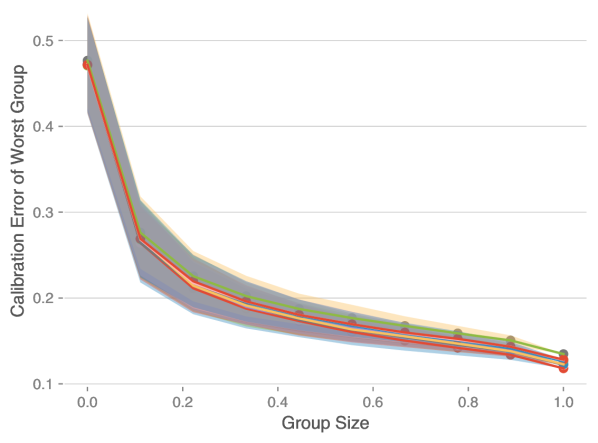
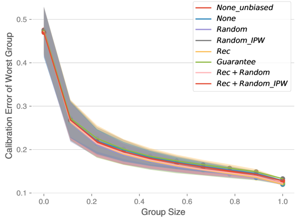
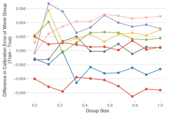
causal_blind
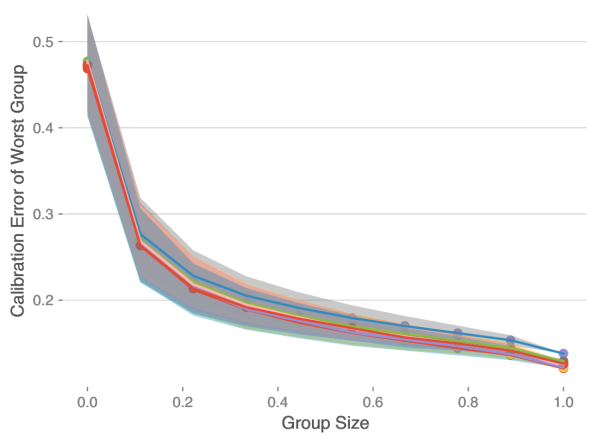
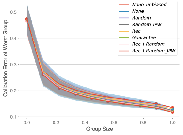
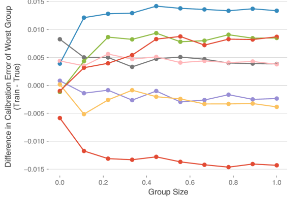
causal_linked
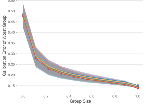
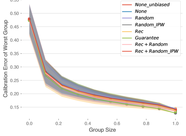
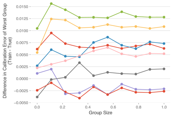
causal_equal

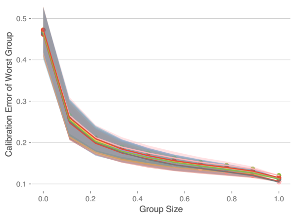
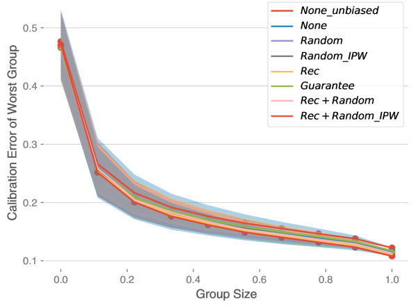
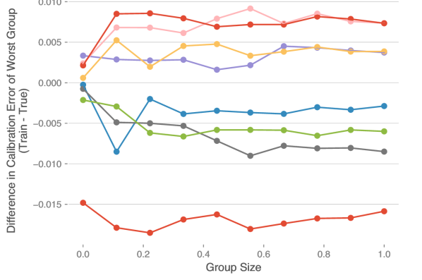
Figure 11. Scatterplots of Root Mean Squared Adversarial Group Calibration Error. To further demonstrate difficulty in detection, we show the adversarial group calibration averaged across all replicates for a given period and then averaged across all periods. In addition we plot one standard deviation above and below. Group size refers to the proportion of test dataset size. For ’Training’, we calculate this metric on the training accumulate at each period. For ’True’, we calculate this metric on a unbiased sample drawn from the entire population. For ease of comparison, we plot the difference between the training and true metric. Overall, we observe little difference in the root mean squared adversarial group error, highlight the difficulty in detecting censoring.

DGP	Train (Observed)	True	Difference (Train - True)
mixed_proxy
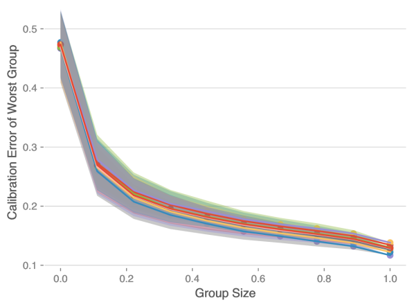
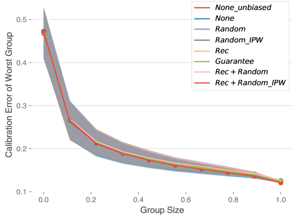
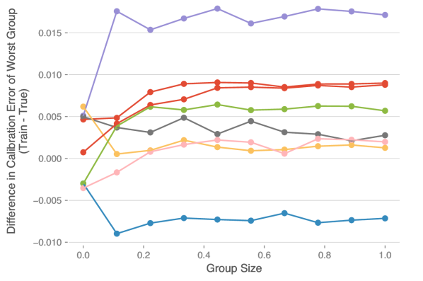
mixed_downstream
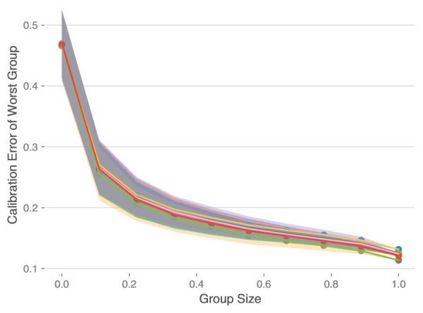
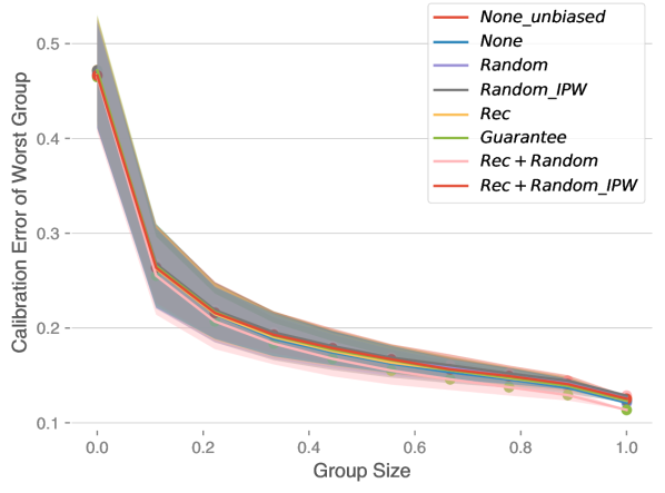
gaming
german

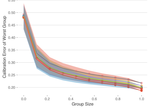
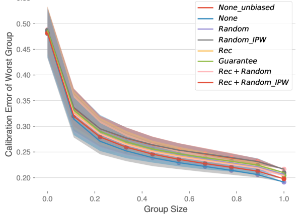
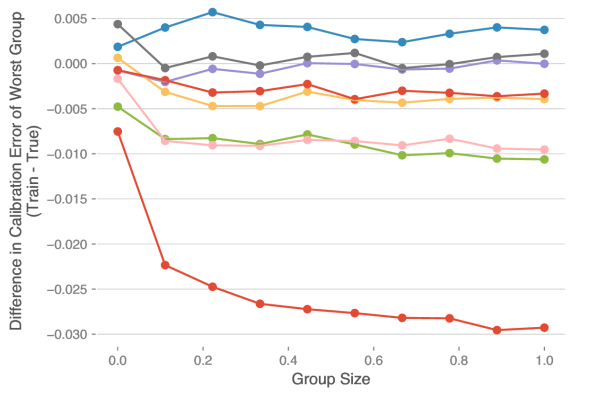
Figure 12. Scatterplots of Root Mean Squared Adversarial Group Calibration Error (contd)

References

- (1)
- UK_([n. d.]) [n. d.]. Digital Regulation: Driving growth and unlocking innovation. https://www.gov.uk/government/publications/digital-regulation-driving-growth-and-unlocking-innovation/digital-regulation-driving-growth-and-unlocking-innovation
- FHA ([n. d.]) [n. d.]. Housing discrimination under the Fair Housing Act. https://www.hud.gov/program_offices/fair_housing_equal_opp/fair_housing_act_overview
- ECO (2021) 2021. The Equal Credit Opportunity Act. https://www.justice.gov/crt/equal-credit-opportunity-act-3
- fdi (2021) 2021. Iv. fair lending —fair lending laws and regulations. https://www.fdic.gov/resources/supervision-and-examinations/consumer-compliance-examination-manual/documents/4/iv-1-1.pdf
- noc (2022) 2022. https://www.experian.com/blogs/ask-experian/no-credit-cause-for-declination-not-lack-of-score/
- US_(2022) 2022. Blueprint for an AI bill of rights. https://www.whitehouse.gov/ostp/ai-bill-of-rights/
- Aka et al. (2021) Osman Aka, Ken Burke, Alex Bauerle, Christina Greer, and Margaret Mitchell. 2021. Measuring model biases in the absence of ground truth. In Proceedings of the 2021 AAAI/ACM Conference on AI, Ethics, and Society. 327–335.
- Akinwumi et al. (2022) Michael Akinwumi, John Merrill, Lisa Rice, Kareem Saleh, and Maureen Yap. 2022. An ai fair lending policy agenda for the Federal Financial Regulators. https://www.brookings.edu/research/an-ai-fair-lending-policy-agenda-for-the-federal-financial-regulators/
- Alliance (2012) National Fair Housing Alliance. 2012. The Banks Are Back, Our Neighborhoods Are Not: Discrimination in the Maintenance and Marketing of REO Properties.
- Baunach (1980) Phyllis Jo Baunach. 1980. RANDOM ASSIGNMENT IN CRIMINAL JUSTICE RESEARCH Some Ethical and Legal Issues. Criminology 17, 4 (1980), 435–444.
- Bechavod et al. (2021) Yahav Bechavod, Katrina Ligett, Steven Wu, and Juba Ziani. 2021. Gaming Helps! Learning from Strategic Interactions in Natural Dynamics. In International Conference on Artificial Intelligence and Statistics. PMLR, 1234–1242.
- Bechavod et al. (2020) Yahav Bechavod, Katrina Ligett, Zhiwei Steven Wu, and Juba Ziani. 2020. Causal feature discovery through strategic modification. arXiv preprint arXiv:2002.07024 3 (2020).
- Bergen et al. (2019) Karianne J Bergen, Paul A Johnson, Maarten V de Hoop, and Gregory C Beroza. 2019. Machine learning for data-driven discovery in solid Earth geoscience. Science 363, 6433 (2019), eaau0323.
- Bhutta et al. (2022) Neil Bhutta, Aurel Hizmo, and Daniel Ringo. 2022. How much does racial bias affect mortgage lending? Evidence from human and algorithmic credit decisions. (2022).
- Blattner and Nelson (2021) Laura Blattner and Scott Nelson. 2021. How Costly is Noise? Data and Disparities in Consumer Credit. arXiv preprint arXiv:2105.07554 (2021).
- Blum and Stangl (2019) Avrim Blum and Kevin Stangl. 2019. Recovering from biased data: Can fairness constraints improve accuracy? arXiv preprint arXiv:1912.01094 (2019).
- Brevoort et al. (2015) Kenneth P Brevoort, Philipp Grimm, and Michelle Kambara. 2015. Data Point: Credit Invisibles.
- Brown et al. (2020) Gavin Brown, Shlomi Hod, and Iden Kalemaj. 2020. Performative Prediction in a Stateful World. arXiv preprint arXiv:2011.03885 (2020).
- Chandak et al. (2020) Yash Chandak, Georgios Theocharous, Blossom Metevier, and Philip Thomas. 2020. Reinforcement learning when all actions are not always available. In Proceedings of the AAAI Conference on Artificial Intelligence, Vol. 34. 3381–3388.
- Chen et al. (2017) Ching-Hui Chen, Vishal M Patel, and Rama Chellappa. 2017. Learning from ambiguously labeled face images. IEEE Transactions on Pattern Analysis and Machine Intelligence 40, 7 (2017), 1653–1667.
- Chen et al. (2019) Yiling Chen, Yang Liu, and Chara Podimata. 2019. Learning strategy-aware linear classifiers. arXiv preprint arXiv:1911.04004 (2019).
- Chen et al. (2020) Yatong Chen, Jialu Wang, and Yang Liu. 2020. Strategic Recourse in Linear Classification. arXiv preprint arXiv:2011.00355 (2020).
- Chung et al. (2021) Youngseog Chung, Ian Char, Han Guo, Jeff Schneider, and Willie Neiswanger. 2021. Uncertainty Toolbox: an Open-Source Library for Assessing, Visualizing, and Improving Uncertainty Quantification. arXiv preprint arXiv:2109.10254 (2021).
- Colli et al. (2014) Agostino Colli, Luigi Pagliaro, and Piergiorgio Duca. 2014. The ethical problem of randomization. Internal and emergency medicine 9, 7 (2014), 799–804.
- Coston et al. (2021) Amanda Coston, Ashesh Rambachan, and Alexandra Chouldechova. 2021. Characterizing fairness over the set of good models under selective labels. In International Conference on Machine Learning. PMLR, 2144–2155.
- Dai (2020) J. Dai. 2020. Label Bias, Label Shift: Fair Machine Learning with Unreliable Labels.
- D’Amour et al. (2020) Alexander D’Amour, Hansa Srinivasan, James Atwood, Pallavi Baljekar, D Sculley, and Yoni Halpern. 2020. Fairness is not static: deeper understanding of long term fairness via simulation studies. In Proceedings of the 2020 Conference on Fairness, Accountability, and Transparency. 525–534.
- Das (2021) Sejuti Das. 2021. Top AI Tools for Resume Screening. Opinions (January 2021). https://analyticsindiamag.com/top-ai-tools-for-resume-screening/
- De-Arteaga et al. (2018) Maria De-Arteaga, Artur Dubrawski, and Alexandra Chouldechova. 2018. Learning under selective labels in the presence of expert consistency. arXiv preprint arXiv:1807.00905 (2018).
- Dobbie et al. (2021) Will Dobbie, Andres Liberman, Daniel Paravisini, and Vikram Pathania. 2021. Measuring bias in consumer lending. The Review of Economic Studies 88, 6 (2021), 2799–2832.
- Elkan and Noto (2008) Charles Elkan and Keith Noto. 2008. Learning classifiers from only positive and unlabeled data. In Proceedings of the 14th ACM SIGKDD international conference on Knowledge discovery and data mining. 213–220.
- Engler (2021a) Alex Engler. 2021a. Independent auditors are struggling to hold AI companies accountable. Fast Company (January 2021), https://www.fastcompany.com/90597594/ai–algorithm–auditing–hirevue.
- Engler (2021b) Alex Engler. 2021b. We’re using AI more and more for hiring. How can we ensure it’s fair? The Brookings Institution (June 2021), https://www.weforum.org/agenda/2021/06/auditing–employment–algorithms–discrimination–fairness/.
- Ensign et al. (2017) Danielle Ensign, Sorelle A Friedler, Scott Neville, Carlos Scheidegger, and Suresh Venkatasubramanian. 2017. Decision making with limited feedback: Error bounds for recidivism prediction and predictive policing. PMLR.
- Ensign et al. (2018) Danielle Ensign, Sorelle A Friedler, Scott Neville, Carlos Scheidegger, and Suresh Venkatasubramanian. 2018. Runaway feedback loops in predictive policing. In Conference on Fairness, Accountability and Transparency. PMLR, 160–171.
- Erdélyi et al. (2021) Gábor Erdélyi, Olivia J Erdélyi, and Vladimir Estivill-Castro. 2021. Randomized Classifiers vs Human Decision-Makers: Trustworthy AI May Have to Act Randomly and Society Seems to Accept This. arXiv preprint arXiv:2111.07545 (2021).
- Goldstein et al. (2018) Cory E Goldstein, Charles Weijer, Jamie C Brehaut, Dean A Fergusson, Jeremy M Grimshaw, Austin R Horn, and Monica Taljaard. 2018. Ethical issues in pragmatic randomized controlled trials: a review of the recent literature identifies gaps in ethical argumentation. BMC medical ethics 19, 1 (2018), 1–10.
- Greer (2012) JL Greer. 2012. Race and mortgage redlining in the United States. In Western political science association meetings. Portland, Oregon.
- Gu and Oelke (2019) Jindong Gu and Daniela Oelke. 2019. Understanding bias in machine learning. arXiv preprint arXiv:1909.01866 (2019).
- Hashimoto et al. (2018) Tatsunori Hashimoto, Megha Srivastava, Hongseok Namkoong, and Percy Liang. 2018. Fairness without demographics in repeated loss minimization. In International Conference on Machine Learning. PMLR, 1929–1938.
- Havard (2005) Cassandra Jones Havard. 2005. To Lend or Not to Lend What the CRA Ought to Say about Sub-Prime and Predatory Lending. Fla. Coastal L. Rev. 7 (2005), 1.
- Hu and Chen (2018) Lily Hu and Yiling Chen. 2018. A short-term intervention for long-term fairness in the labor market. In Proceedings of the 2018 World Wide Web Conference. 1389–1398.
- Hu et al. (2021) Wenpeng Hu, Ran Le, Bing Liu, Feng Ji, Jinwen Ma, Dongyan Zhao, and Rui Yan. 2021. Predictive adversarial learning from positive and unlabeled data. In Proceedings of the AAAI Conference on Artificial Intelligence, Vol. 35. 7806–7814.
- Immorlica et al. (2018) Nicole Immorlica, Jieming Mao, Aleksandrs Slivkins, and Zhiwei Steven Wu. 2018. Incentivizing exploration with selective data disclosure. arXiv preprint arXiv:1811.06026 (2018).
- Jiang et al. (2021) Heinrich Jiang, Qijia Jiang, and Aldo Pacchiano. 2021. Learning the truth from only one side of the story. In International Conference on Artificial Intelligence and Statistics. PMLR, 2413–2421.
- Kagan (2020) Julia Kagan. 2020. Equal Credit Opportunity Act (ECOA). Investopedia (2020).
- Kallus and Zhou (2018) Nathan Kallus and Angela Zhou. 2018. Residual Unfairness in Fair Machine Learning from Prejudiced Data. In International Conference on Machine Learning.
- Karimi et al. (2020a) Amir-Hossein Karimi, Gilles Barthe, Bernhard Schölkopf, and Isabel Valera. 2020a. A survey of algorithmic recourse: definitions, formulations, solutions, and prospects. arXiv preprint arXiv:2010.04050 (2020).
- Karimi et al. (2020b) Amir-Hossein Karimi, Julius von Kügelgen, Bernhard Schölkopf, and Isabel Valera. 2020b. Algorithmic recourse under imperfect causal knowledge: a probabilistic approach. arXiv preprint arXiv:2006.06831 (2020).
- Kelley and Ovchinnikov (2021) Stephanie Kelley and Anton Ovchinnikov. 2021. Anti-discrimination Laws, AI, and Gender Bias: A Case Study in Non-mortgage Fintech Lending. AI, and Gender Bias: A Case Study in Non-mortgage Fintech Lending (September 27, 2021) (2021).
- Khanal and Kanan (2021) Bidur Khanal and Christopher Kanan. 2021. How Does Heterogeneous Label Noise Impact Generalization in Neural Nets?. In International Symposium on Visual Computing. Springer, 229–241.
- Kilbertus et al. (2020) N. Kilbertus, M. Gomez Rodriguez, B. Schölkopf, K. Muandet, and I. Valera. 2020. Fair Decisions Despite Imperfect Predictions. In Proceedings of the 23rd International Conference on Artificial Intelligence and Statistics (AISTATS) (Proceedings of Machine Learning Research, Vol. 108). PMLR, 277–287. http://proceedings.mlr.press/v108/kilbertus20a.html
- Kozodoi et al. (2021) Nikita Kozodoi, Johannes Jacob, and Stefan Lessmann. 2021. Fairness in Credit Scoring: Assessment, Implementation and Profit Implications. arXiv preprint arXiv:2103.01907 (2021).
- Krauth et al. (2020) Karl Krauth, Sarah Dean, Alex Zhao, Wenshuo Guo, Mihaela Curmei, Benjamin Recht, and Michael I Jordan. 2020. Do Offline Metrics Predict Online Performance in Recommender Systems? arXiv preprint arXiv:2011.07931 (2020).
- Kuleshov et al. (2018) Volodymyr Kuleshov, Nathan Fenner, and Stefano Ermon. 2018. Accurate uncertainties for deep learning using calibrated regression. In International conference on machine learning. PMLR, 2796–2804.
- Kulkarni and Neth (2020) Kshitij Kulkarni and Sven Neth. 2020. Social Choice with Changing Preferences: Representation Theorems and Long-Run Policies. arXiv preprint arXiv:2011.02544 (2020).
- Kumar et al. (2022) I Elizabeth Kumar, Keegan E Hines, and John P Dickerson. 2022. Equalizing Credit Opportunity in Algorithms: Aligning Algorithmic Fairness Research with US Fair Lending Regulation. In Proceedings of the 2022 AAAI/ACM Conference on AI, Ethics, and Society. 357–368.
- Lakkaraju et al. (2017) Himabindu Lakkaraju, Jon Kleinberg, Jure Leskovec, Jens Ludwig, and Sendhil Mullainathan. 2017. The selective labels problem: Evaluating algorithmic predictions in the presence of unobservables. In Proceedings of the 23rd ACM SIGKDD International Conference on Knowledge Discovery and Data Mining. 275–284.
- Lee and Liu (2003) Wee Sun Lee and Bing Liu. 2003. Learning with positive and unlabeled examples using weighted logistic regression. In ICML, Vol. 3. 448–455.
- Levanon and Rosenfeld (2021) Sagi Levanon and Nir Rosenfeld. 2021. Strategic Classification Made Practical. arXiv preprint arXiv:2103.01826 (2021).
- Li et al. (2020) Danielle Li, Lindsey R Raymond, and Peter Bergman. 2020. Hiring as Exploration. Technical Report. National Bureau of Economic Research.
- Liu et al. (2018) Lydia T. Liu, Sarah Dean, Esther Rolf, Max Simchowitz, and Moritz Hardt. 2018. Delayed Impact of Fair Machine Learning. CoRR abs/1803.04383 (2018). arXiv:1803.04383 http://arxiv.org/abs/1803.04383
- Lum and Isaac (2016) Kristian Lum and William Isaac. 2016. To predict and serve? Significance 13, 5 (2016), 14–19.
- Mansour et al. (2021) Yishay Mansour, Alex Slivkins, Vasilis Syrgkanis, and Zhiwei Steven Wu. 2021. Bayesian exploration: Incentivizing exploration in bayesian games. Operations Research (2021).
- Miller et al. (2020) John Miller, Smitha Milli, and Moritz Hardt. 2020. Strategic classification is causal modeling in disguise. In International Conference on Machine Learning. PMLR, 6917–6926.
- Milli et al. (2019) Smitha Milli, John Miller, Anca D Dragan, and Moritz Hardt. 2019. The social cost of strategic classification. In Proceedings of the Conference on Fairness, Accountability, and Transparency. 230–239.
- Pollice et al. (2021) Robert Pollice, Gabriel dos Passos Gomes, Matteo Aldeghi, Riley J Hickman, Mario Krenn, Cyrille Lavigne, Michael Lindner-D’Addario, AkshatKumar Nigam, Cher Tian Ser, Zhenpeng Yao, et al. 2021. Data-driven strategies for accelerated materials design. Accounts of Chemical Research 54, 4 (2021), 849–860.
- Press ([n. d.]) Daniel Press. [n. d.]. The CFPB and the Equal Credit Opportunity Act. Competitive Enterprise Institute, On Point ([n. d.]).
- Quiñonero-Candela et al. (2009) Joaquin Quiñonero-Candela, Masashi Sugiyama, Neil D Lawrence, and Anton Schwaighofer. 2009. Dataset shift in machine learning. Mit Press.
- Raccuglia et al. (2016) Paul Raccuglia, Katherine C Elbert, Philip DF Adler, Casey Falk, Malia B Wenny, Aurelio Mollo, Matthias Zeller, Sorelle A Friedler, Joshua Schrier, and Alexander J Norquist. 2016. Machine-learning-assisted materials discovery using failed experiments. Nature 533, 7601 (2016), 73–76.
- Raghavan et al. (2020) Manish Raghavan, Solon Barocas, Jon Kleinberg, and Karen Levy. 2020. Mitigating bias in algorithmic hiring: Evaluating claims and practices. In Proceedings of the 2020 conference on fairness, accountability, and transparency. 469–481.
- Rateike et al. (2022) Miriam Rateike, Ayan Majumdar, Olga Mineeva, Krishna P Gummadi, and Isabel Valera. 2022. Don’t Throw it Away! The Utility of Unlabeled Data in Fair Decision Making. In 2022 ACM Conference on Fairness, Accountability, and Transparency. 1421–1433.
- Rawal et al. (2020) Kaivalya Rawal, Ece Kamar, and Himabindu Lakkaraju. 2020. Can I Still Trust You?: Understanding the Impact of Distribution Shifts on Algorithmic Recourses. arXiv preprint arXiv:2012.11788 (2020).
- Rice and Swesnik (2013) Lisa Rice and Deidre Swesnik. 2013. Discriminatory effects of credit scoring on communities of color. Suffolk UL Rev. 46 (2013), 935.
- Ross et al. (2021) Alexis Ross, Himabindu Lakkaraju, and Osbert Bastani. 2021. Learning Models for Actionable Recourse. Advances in Neural Information Processing Systems 34 (2021).
- Royall (1991) Richard M Royall. 1991. Ethics and statistics in randomized clinical trials. Statist. Sci. 6, 1 (1991), 52–62.
- Sengupta and Shrestha (2019) Partho P Sengupta and Sirish Shrestha. 2019. Machine learning for data-driven discovery: the rise and relevance. , 690–692 pages.
- Shavit et al. (2020) Yonadav Shavit, Benjamin Edelman, and Brian Axelrod. 2020. Learning from strategic agents: Accuracy, improvement, and causality. arXiv preprint arXiv:2002.10066 (2020).
- Shimodaira (2000) Hidetoshi Shimodaira. 2000. Improving predictive inference under covariate shift by weighting the log-likelihood function. Journal of statistical planning and inference 90, 2 (2000), 227–244.
- Simchowitz and Slivkins (2021) Max Simchowitz and Aleksandrs Slivkins. 2021. Exploration and Incentives in Reinforcement Learning. arXiv preprint arXiv:2103.00360 (2021).
- Soenksen et al. (2021) Luis R Soenksen, Timothy Kassis, Susan T Conover, Berta Marti-Fuster, Judith S Birkenfeld, Jason Tucker-Schwartz, Asif Naseem, Robert R Stavert, Caroline C Kim, Maryanne M Senna, et al. 2021. Using deep learning for dermatologist-level detection of suspicious pigmented skin lesions from wide-field images. Science Translational Medicine 13, 581 (2021), eabb3652.
- Squires (2017) Gregory D Squires. 2017. The fight for fair housing: Causes, consequences, and future implications of the 1968 Federal Fair Housing Act. Routledge.
- Tran et al. (2020) Kevin Tran, Willie Neiswanger, Junwoong Yoon, Qingyang Zhang, Eric Xing, and Zachary W Ulissi. 2020. Methods for comparing uncertainty quantifications for material property predictions. Machine Learning: Science and Technology 1, 2 (2020), 025006.
- Upadhyay et al. (2021) Sohini Upadhyay, Shalmali Joshi, and Himabindu Lakkaraju. 2021. Towards Robust and Reliable Algorithmic Recourse. arXiv preprint arXiv:2102.13620 (2021).
- Ustun et al. (2019) Berk Ustun, Alexander Spangher, and Yang Liu. 2019. Actionable recourse in linear classification. In Proceedings of the Conference on Fairness, Accountability, and Transparency. 10–19.
- Veit et al. (2017) Andreas Veit, Neil Alldrin, Gal Chechik, Ivan Krasin, Abhinav Gupta, and Serge Belongie. 2017. Learning from noisy large-scale datasets with minimal supervision. In Proceedings of the IEEE conference on computer vision and pattern recognition. 839–847.
- Venkatasubramanian and Alfano (2020) Suresh Venkatasubramanian and Mark Alfano. 2020. The philosophical basis of algorithmic recourse. In Proceedings of the 2020 Conference on Fairness, Accountability, and Transparency. 284–293.
- von Kügelgen et al. (2020) Julius von Kügelgen, Umang Bhatt, Amir-Hossein Karimi, Isabel Valera, Adrian Weller, and Bernhard Schölkopf. 2020. On the fairness of causal algorithmic recourse. arXiv preprint arXiv:2010.06529 (2020).
- Wei (2020) Dennis Wei. 2020. Optimal Policies for the Homogeneous Selective Labels Problem. arXiv preprint arXiv:2011.01381 (2020).
- Wei et al. (2021) Jiaheng Wei, Zhaowei Zhu, Hao Cheng, Tongliang Liu, Gang Niu, and Yang Liu. 2021. Learning with noisy labels revisited: A study using real-world human annotations. arXiv preprint arXiv:2110.12088 (2021).
- Yan et al. (2014) Yan Yan, Rómer Rosales, Glenn Fung, Ramanathan Subramanian, and Jennifer Dy. 2014. Learning from multiple annotators with varying expertise. Machine learning 95, 3 (2014), 291–327.
- Zhang et al. (2021) Yikai Zhang, Songzhu Zheng, Pengxiang Wu, Mayank Goswami, and Chao Chen. 2021. Learning with feature-dependent label noise: A progressive approach. arXiv preprint arXiv:2103.07756 (2021).
- Zhao et al. (2022) Sendong Zhao, Aobo Wang, Bing Qin, and Fei Wang. 2022. Biomedical evidence engineering for data-driven discovery. Bioinformatics 38, 23 (2022), 5270–5278.