Alexander Moreno Jonathan Mei^∗ Luke Walters^∗
{alexander.f.moreno,jonathanmei,lukecwalters}@gmail.com All authors contributed equally. Alexander and Jonathan flipped for ordering. The vast majority of this work was done while the authors were at Luminous Computing.

SKI to go Faster: Accelerating Toeplitz Neural Networks via Asymmetric Kernels

Alexander Moreno Jonathan Mei^∗ Luke Walters^∗
{alexander.f.moreno,jonathanmei,lukecwalters}@gmail.com All authors contributed equally. Alexander and Jonathan flipped for ordering. The vast majority of this work was done while the authors were at Luminous Computing.

Abstract

Toeplitz Neural Networks (TNNs) Qin et al. (2023) are a recent impressive sequence model requiring $O(n\log n)$ computational complexity and $O(n)$ relative positional encoder (RPE) multi-layer perceptron (MLP) and decay bias calls. We aim to reduce both. We first note that the RPE is a non symmetric positive definite kernel and the Toeplitz matrices are pseudo-Gram matrices. Further 1) the learned kernels display spiky behavior near the main diagonals with otherwise smooth behavior; 2) the RPE MLP is slow. For bidirectional models, this motivates a sparse plus low-rank Toeplitz matrix decomposition. For the sparse component’s action, we do a small 1D convolution. For the low rank component, we replace the RPE MLP with linear interpolation and use Structured Kernel Interpolation (SKI) Wilson and Nickisch (2015) for $O(n)$ complexity. For causal models, “fast” causal masking Katharopoulos et al. (2020) negates SKI’s benefits. Working in frequency domain, we avoid an explicit decay bias. To enforce causality, we represent the kernel via the real part of its frequency response using the RPE and compute the imaginary part via a Hilbert transform. This maintains $O(n\log n)$ complexity but achieves an absolute speedup. Modeling the frequency response directly is also competitive for bidirectional training, using one fewer FFT. We improve on speed and sometimes score on the Long Range Arena (LRA) Tay et al. (2020).

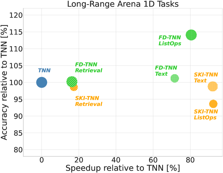
(a) Long Range Arena (LRA).

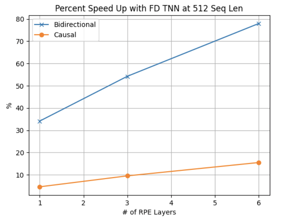
(b) Pre-training speedups using Fourier Domain.

Figure 1: (a) In LRA, our approaches, SKI and FD-TNN are faster than TNNs for 1d tasks with strong LRA scores. Bubble sizes denote training model memory. (b) Our approach, FD-TNN, achieves substantial speed ups in iterations/sec for pre-training both causal and bidirectional models. Note that we do not include SKI-TNN in this plot as it does not use an MLP based RPE.

1 Introduction

Sequence modeling is important in natural language processing, where sentences are represented as a sequence of tokens. Successful sequence modeling typically involves token and channel mixing. Token mixing combines representations of different sequence parts, while channel mixing combines the information across different dimensions of embedding vectors used to encode tokens. Transformers Vaswani et al. (2017) are arguably the most successful technique for sequence modeling, and variants including Hoffmann et al. (2022); Clark et al. (2020) have achieved state of the art performance on natural language tasks. They use self-attention for token mixing and feedforward networks for channel mixing.

Recently, Qin et al. (2023) proposed Toeplitz Neural Networks (TNN) using Toeplitz matrices for token mixing. They use a learned neural similarity function, the Relative Positional Encoder (RPE), to form the Toeplitz matrices. Toeplitz matrix vector multiplication can be performed with sub-quadratic complexity using the Fast Fourier Transform (FFT), giving the TNN token mixing layer a total $O(dn\log n)$ computational complexity, where $d$ is the embedding dimension and $n$ is the sequence length. This achieved state of the art predictive performance and nearly state of the art speed for the long range arena (LRA) benchmark Tay et al. (2020). They also showed strong performance pre-training wikitext-103 Merity et al. (2016) and on the GLUE benchmarkWang et al. (2019). Despite strong empirical speed performance, TNNs have two fundamental efficiency limitations: 1) super-linear computational complexity 2) many calls to the RPE: for each layer, one call per relative position.

In this paper, we interpret the RPE as a non-SPD kernel and note 1) the learned kernels are discontinuous near the main diagonals but otherwise smooth globally; 2) the ReLU RPE learns 1D piecewise linear functions: an MLP is slower than necessary. For bidirectional models, this motivates a sparse plus low-rank decomposition. We apply the sparse component’s action via a small 1D convolution. For the low rank component, we replace the RPE MLP with linear interpolation at a set of inducing points and an asymmetric extension of Structured Kernel Interpolation (SKI) Wilson and Nickisch (2015) for $O(n)$ complexity. Further, using an inverse time warp, we can extrapolate beyond sequence lengths observed during training. For causal models, even “fast” causal masking Katharopoulos et al. (2020) negates the speed and memory benefits from SKI. Thus, we instead represent the real part of the kernel’s frequency response using the RPE MLP, and evaluate the RPE with finer frequency resolution to extrapolate to longer sequence lengths in the time domain. From the real part, we compute the imaginary part via a Hilbert transform during the forward pass to enforce causality. In the bidirectional setting, we remove the causality constraint and represent the complex frequency response of the kernel with the RPE MLP. Levels of smoothness in frequency response imply decay rates in the time domain: thus we model the decay bias implicitly. This maintains $O(n\log n)$ complexity but achieves an absolute speedup. Further, it often leads to better predictive performance on LRA tasks.

This paper has three primary contributions: 1) a TNN sparse plus low rank decomposition, extending SKI to TNNs for the low rank part. We replace the RPE MLP with linear interpolation and apply inverse time warping to efficiently train bidirectional TNNs. We provide rigorous error analysis for our asymmetric SKI application; 2) alternatively, for both causal and bidirectional models, we work directly in the frequency domain and use the Hilbert transform to enforce causality in the autoregressive setting. We prove that different activation choices for an MLP modeling the discrete time Fourier transform (DTFT) lead to different decay rates in the original kernel. 3) Empirical results: we demonstrate that our approaches show dramatically improved computational efficiency, setting a new speed state of the art on LRA Tay et al. (2022) on the 1d tasks, with strong LRA score. In section 2 we describe related work. In section 3 we propose our new modeling approaches. In 4 we state several theoretical results regarding our modeling approaches. In 5 we extend the empirical results of Qin et al. (2023), showing our speed gains with minimal prediction deterioration. We conclude in section 7.

2 Related

The most related papers use Toeplitz matrices for sequence modeling Qin et al. (2023); Luo et al. (2021); Poli et al. (2023). We build off of Qin et al. (2023) and introduce several techniques to improve on their speed results. Luo et al. (2021) took a similar approach, but applied Toeplitz matrices to self-attention rather than departing from it. Poli et al. (2023) is also similar, using alternating Toeplitz and diagonal matrices as a replacement for self-attention within a Transformer. While we focus on the setting of Qin et al. (2023) as it was released first, our approach is applicable to Poli et al. (2023).

Also related are kernel based xFormers, particularly those using the Nyström method Nyström (1930); Baker (1977). The most related work is Xiong et al. (2021), which adapts a matrix Nyström method for asymmetric matrices Nemtsov et al. (2016) to self-attention. We instead adapt this along with SKI Wilson and Nickisch (2015) to Toeplitz matrices. Chen et al. (2021) extends Xiong et al. (2021) by embedding the self-attention matrix into a larger PSD kernel matrix and approximating the larger matrix instead. Their final approximate matrix has lower spectral error compared to Xiong et al. (2021) and higher average validation accuracy on LRA Tay et al. (2020). However, their method is slightly slower. Also somewhat related are random feature self-attention approximationsPeng et al. (2021); Choromanski et al. (2021). These extend Rahimi and Recht (2007), but use different random features that better approximate self-attention than random Fourier or binning features.

Sparse transformers are also relevant. Child et al. (2019) proposed using strided and fixed patterns. Brown et al. (2020) alternated between sparse locally banded and dense attention. Finally, Zaheer et al. (2020) proposed combining random attention, window attention and global attention. Our use of a short convolutional filter is most similar to window attention. The space of efficient transformers is huge and there are many models that we haven’t covered that may be relevant. Tay et al. (2022) provides an excellent survey.

Other successful long sequence approaches include state space models Gu et al. (2022); Smith et al. (2023); Dao et al. (2022), long convolution Romero et al. (2022); Fu et al. (2023), adding moving averages to gated attention Ma et al. (2023) and more Khalitov et al. (2023).

3 Modeling Approach

We review Toeplitz neural networks (TNNs) in section 3.1. We next speed up the TNN’s Toeplitz neural operator (TNO). We discuss using Nyström and SKI approaches to bidirectional training in 3.2. We discuss frequency based approaches, particularly for causal training in 3.3.

3.1 Preliminaries: Toeplitz matrices and Toeplitz Neural Networks

TNNs Qin et al. (2023) replace self-attention, which computes the action of self-attention matrices that encode the similarity between both observation values and absolute positions, with the action of Toeplitz matrices that encode similarity only based on relative positions. Toeplitz matrices have, for each diagonal, the same entries from left to right. That is, $\mathbf{T}_{ij}=t_{i-j},\mathbf{T}\in\mathbb{R}^{n\times n}$. Unlike self-attention matrices, which require $O(n^{2})$ memory, a Toeplitz matrix has $2n-1$ unique elements and requires $O(n)$ memory. Due to close connections with discrete-time convolution, $\mathbf{T}\mathbf{x}$ can be computed in $O(n\log n)$ time by embedding $\mathbf{T}$ in a circulant matrix and applying FFT.

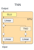
(a) TNN architecture.

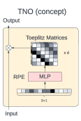
(b) TNO module.

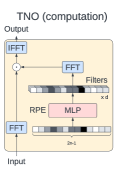
(c) Fast computations to implement TNO.

Figure 3: Toeplitz Neural Network and Toeplitz Neural Operators: (a) The overall architecture of a TNN layer Qin et al. [2023]. (b) Conceptually, the TNO multiplies each channel of the input by a different Toeplitz matrix. (c) Computationally, the TNO uses FFT’s for speed.

A TNN Qin et al. (2023) has multiple sequence modeling blocks, which we show in Figure 3 in Appendix A. Each block has a Gated Toeplitz Unit (GTU), which does both token and channel mixing, followed by a Gated Linear Unit (GLU) Shazeer (2020), which does channel mixing. The core of the GTU is the Toeplitz Neural Operator (TNO), which does token mixing and is the part of the architecture that we modify.

(a) SKI-TNO.

(b) Fast implementation of SKI-TNO.

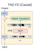
(c) FD-TNO causal.

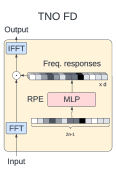
(d) FD-TNO bidirectional.

Figure 2: Our SKI-TNO and FD-TNO modifications: (a) We decompose Toeplitz matrices into sums of sparse + smooth components. Additionally, we use interpolation instead of an MLP to learn the RPE. (b) We use a 1D convolution to apply the sparse component and SKI as a low-rank approximation to the smooth component. (c) For the causal case, we use frequency domain RPE with a Hilbert Transform to enforce causality. (d) Our FD-TNO also is competitive in the bidirectional case, with one fewer FFT than TNO.

We now describe the TNO, shown in Figure 3(b) of Appendix A. Given a sequence $\mathbf{X}\in\mathbb{R}^{n\times d}$ of length $n$ and dimension $d$ in discrete time, there are $2n-1$ unique relative positions/times $i-j$ for $i,j=1,\ldots,n$. An $\textrm{RPE}:\mathbb{Z}\rightarrow\mathbb{R}^{d}$ neural network maps each relative position to a $d$-dimensional embedding. These embeddings are used to construct Toeplitz matrices $\mathbf{T}^{l}$ for $l=1,\ldots,d$ using

$$\mathbf{T}^{l}_{ij} =\lambda^{|i-j|}\textrm{RPE}_{l}(i-j).$$

$\textrm{RPE}_{l}(i-j)$ is a learned similarity between positions for dimension $l$, while $\lambda^{|i-j|}$ with $\lambda\in(0,1)$ is an exponential decay bias penalizing far away tokens to be dissimilar. We can interpret $\mathbf{T}^{l}_{ij}$ as evaluating a stationary non-SPD kernel $k_{l}(i-j)=\lambda^{|i-j|}\textrm{RPE}_{l}(i-j)$. Thus $\mathbf{T}^{l}$ can be interpreted as a pseudo or generalized Gram matrix. Letting $\mathbf{x}^{l}$ be the $l$th column of $\mathbf{X}$, the TNO outputs

$$\textrm{TNO}(\mathbf{X}) =(\mathbf{T}^{1}\mathbf{x}^{1}\ldots\mathbf{T}^{d}\mathbf{x}^{d})\in\mathbb{R}^{n\times d}$$

where each $\mathbf{T}^{l}\mathbf{x}^{l}$ is computed via the FFT as described above.

The main costs are the RPE’s MLP, the FFT, and the decay bias. We aim to eliminate the MLP and decay bias when possible. In the bidirectional setting, we use SKI to apply the FFT using a much smaller Toeplitz matrix. In a separate model we learn the RPE’s frequency response directly. In the bidirectional setting, this allows us to both avoid explicitly modeling the decay bias and use one fewer FFT. In the causal setting, it allows us to avoid explicitly modeling the decay bias.

3.2 SKI Based Approaches for Bidirectional Training

For a given Toeplitz matrix $\mathbf{T}$, we assume it admits a decomposition that we can approximate with a sparse+low-rank representation, $\mathbf{T}=\mathbf{T}_{\textrm{sparse}}+\mathbf{T}_{\textrm{smooth}}\approx\mathbf{T}_{\textrm{sparse}}+\mathbf{T}_{\textrm{low}}$. Our bidirectional training thus consists of three primary components. The first, the sparse component $\mathbf{T}_{\textrm{sparse}}$ is straightforward. Applying the action $\mathbf{T}_{\textrm{sparse}}\mathbf{x}$ of $\mathbf{T}_{\textrm{sparse}}\in\mathbb{R}^{n\times n}$ with $m$ non-zero diagonals is equivalent to applying a 1D convolution layer with filter size $m$. We then discuss our asymmetric SKI for $\mathbf{T}_{\textrm{low}}$ in section 3.2.1. Finally, we discuss how we handle sequence lengths not observed in training for $\mathbf{T}_{\textrm{low}}$ via an inverse time warp in section 3.2.2. Algorithm 1 summarizes our TNO based on these techniques.

Algorithm 1 Sparse Plus Low Rank Bidirectional TNO with Asymmetric SKI

Given sequence $\mathbf{X}\in\mathbb{R}^{n\times d}$ with columns $\mathbf{x}^{l}$

Hyperparameters rank $r\ll n$, sparse filter size $m$, interpolation degree $N$, decay parameter $\lambda$

Compute inducing points $p_{1},\ldots,p_{r}$ evenly spaced on $[0,n]$

for $l=1,\ldots,d$ do

     Compute $\mathbf{T}_{\textrm{sparse}}^{l}\mathbf{x}^{l}$ with a 1D convolutional filter, size $m$.

     Let $x(t)=\textrm{sign}(t)\lambda^{|t|}$.

     Form $\mathbf{A}^{l}\in\mathbb{R}^{r\times r}$ with entries $\mathbf{A}_{ij}^{l}=k_{l}(p_{i}-p_{j})=\textrm{RPE}_{l}(x(p_{i}-p_{j}))$

     Form $\mathbf{W}^{l}\in\mathbb{R}^{n\times r}$ degree $N$ polynomial interpolation matrix

     Compute $\mathbf{T}_{\textrm{low}}^{l}\mathbf{x}^{l}$ with $\mathbf{T}_{\textrm{low}}^{l}=\mathbf{W}^{l}\mathbf{A}^{l}\mathbf{W}^{l\top}$

end for

Return $\textrm{TNO}(\mathbf{X})=(\mathbf{T}_{\textrm{sparse}}^{1}\mathbf{x}^{1}+\mathbf{T}_{\textrm{low}}^{1}\mathbf{x}^{1},\ldots,\mathbf{T}_{\textrm{sparse}}^{d}\mathbf{x}^{d}+\mathbf{T}_{\textrm{low}}^{d}\mathbf{x}^{d})$

3.2.1 SKI For Asymmetric Nyström

Given an asymmetric stationary kernel $k:\mathbb{R}\times\mathbb{R}\rightarrow\mathbb{R}$, we wish to approximate the (pseudo) Gram matrix $\mathbf{T}\in\mathbb{R}^{n\times n}$ using a low-rank approximation based on a smaller Gram matrix $\mathbf{A}\in\mathbb{R}^{r\times r}$, with $r\ll n$. In context, $\mathbf{A}$ is formed using relative positions between a set of inducing points $p_{1},\ldots,p_{r}$ instead of the full set $1,\ldots,n$ that is used for $\mathbf{T}$. That is,

$$\mathbf{T}_{ij}=k(i-j)\qquad\textrm{and}\qquad\mathbf{A}_{ij}=k(p_{i}-p_{j}).$$

In our case, the inducing points are uniformly spaced. Some submatrices of $\mathbf{A}$ may be submatrices of $\mathbf{T}$ (if inducing points are also observation points). To derive the Nyström approximation, we form an augmented Gram matrix $\mathbf{K}\in\mathbb{R}^{(n+r)\times(n+r)}$ in block form as

$$\mathbf{K} =\begin{pmatrix}\mathbf{A}&\mathbf{B}\\ \mathbf{F}&\mathbf{T}\end{pmatrix},$$

where $\mathbf{B}\in\mathbb{R}^{r\times n}$ and $\mathbf{F}\in\mathbb{R}^{n\times r}$ are respectively the upper right and lower left partitions of the large Gram matrix $\mathbf{K}$. Explicitly,

$$\mathbf{B}_{ij}=k(p_{i}-j)\qquad\textrm{and}\qquad\mathbf{F}_{ij}=k(i-p_{j}).$$

Extending Nemtsov et al. (2016) to allow singular $\mathbf{A}$,

$$\widehat{\mathbf{K}} =\begin{pmatrix}\mathbf{A}\\ \mathbf{F}\end{pmatrix}\mathbf{A}^{\dagger}\begin{pmatrix}\mathbf{A}&\mathbf{B}\end{pmatrix}=\begin{pmatrix}\mathbf{A}&\mathbf{A}\mathbf{A}^{\dagger}\mathbf{B}\\ \mathbf{F}\mathbf{A}^{\dagger}\mathbf{A}&\mathbf{F}\mathbf{A}^{\dagger}\mathbf{B}\end{pmatrix}$$

where $\mathbf{A}^{\dagger}$ is the Moore-Penrose pseudo-inverse satisfying $\mathbf{A}\mathbf{A}^{\dagger}\mathbf{A}=\mathbf{A}$ (but not necessarily $\mathbf{A}\mathbf{A}^{\dagger}=\mathbf{I}$ as in Nemtsov et al. (2016), which shows up in our different expressions for off-diagonal blocks of $\widehat{\mathbf{K}}$). Following structured kernel interpolation (SKI) Wilson and Nickisch (2015), we approximate $\mathbf{F}$ and $\mathbf{B}$ using interpolation. Specifically,

$$\mathbf{F}\approx\mathbf{W}\mathbf{A}\qquad\textrm{and}\qquad\mathbf{B}\approx\mathbf{A}\mathbf{W}^{\top}$$

where $\mathbf{W}\in\mathbb{R}^{n\times r}$ is a matrix of sparse interpolation weights with up to two non-zero entries per row for linear interpolation or up to four for cubic. These weights can be computed in closed form from the inducing points $p_{i}$ and the observation points $i$. Thus we have

$$\mathbf{T} \approx\mathbf{F}\mathbf{A}^{\dagger}\mathbf{B}\approx\mathbf{W}\mathbf{A}\mathbf{A}^{\dagger}\mathbf{A}\mathbf{W}^{\top}=\mathbf{W}\mathbf{A}\mathbf{W}^{\top}$$

$$\Rightarrow\widetilde{\mathbf{T}} =\mathbf{W}\mathbf{A}\mathbf{W}^{\top}$$

as desired. We can set $\mathbf{T}_{\textrm{low}}=\tilde{\mathbf{T}}$ and compute $\tilde{\mathbf{T}}\mathbf{x}$ by first applying $\mathbf{W}^{\top}\mathbf{x}$, which is an $O(n)$ operation due to $\mathbf{W}\in\mathbb{R}^{n\times r}$ having sparse rows. Next, we apply $\mathbf{A}(\mathbf{W}^{\top}\mathbf{x})$. Since $\mathbf{A}$ is a Toeplitz matrix, this is $O(r\log r)$ as per Section 3.1. Finally, $\mathbf{W}(\mathbf{A}\mathbf{W}^{\top}\mathbf{x})$, the action of $\mathbf{W}$, is again an $O(n)$ operation. Thus computing $\tilde{\mathbf{T}}\mathbf{x}$ is $O(n+r\log r)$ computation. On a GPU, this factorization achieves a speedup from having small $r$ and being able to leverage efficient parallelized matrix multiplication on specialized hardware. However, in PyTorch Paszke et al. (2019), we note that for medium sized matrices up to $n=512$, the time required for data movement in order to perform sparse-dense matrix multiplications can be higher than that of simply performing dense matrix multiplication. This means that in practice, we may instead choose to perform batched dense matrix multiplication, which yields an absolute speedup but a worse asymptotic complexity of $O(nr^{2}+r\log r)$.

3.2.2 Inverse Time Warp

TNNs use $k_{l}(i-j)=\lambda^{|i-j|}\textrm{RPE}_{l}(i-j)$, where $\textrm{RPE}_{l}(i-j)$ is an MLP. There are two issues: 1) the sequential computations required for an MLP are slow, and we only need to evaluate at $2r-1$ points using SKI instead of $2n-1$ to produce the full matrix; 2) extrapolation is used in extending to longer sequence lengths than the MLP was trained on, which is generally less reliable than interpolation.

In Proposition 1, we note that an MLP $f:\mathbb{R}\rightarrow\mathbb{R}^{d}$ with ReLU activations and layer normalization is $d$ piecewise linear functions. As we only need to evaluate at $2r-1$ points, we could let $\textrm{RPE}_{l}$ be a piecewise linear function with $r$ grid points. However, we still need to handle extrapolation. We use an inverse time warp and let $\textrm{RPE}_{l}$ linearly interpolate on $[-1,1]$ with the constraint $\textrm{RPE}_{l}(0)=0$ and define $x(t)=\textrm{sign}(t)\lambda^{|t|}$ for some $0<\lambda<1$. We then let $k_{l}(i-j)=\textrm{RPE}_{l}(x(i-j))$.

3.3 Frequency Based Approaches

3.3.1 Causal Training

The SKI approach allows training bidirectional TNNs with linear complexity. However, fast causal masking negates SKI’s benefits (see Appendix B). Thus we need an alternate causal speedup. We use an MLP in the Fourier domain to avoid an explicit time domain decay bias, and use the Hilbert transform to enforce causality. We now describe how we can learn a causal kernel when working in frequency domain (FD). We first define the discrete Hilbert transform, the key tool for achieving this.

Definition 1.

The discrete Hilbert transform of the discrete Fourier transform $\hat{k}$ is given by

$$\mathcal{H}\{\hat{k}\} =\hat{k}*h$$

where $*$ denotes convolution and

$$h[l] =\begin{cases}0\textrm{, $l$ even}\\ \frac{2}{\pi l}\textrm{, $l$ odd}\end{cases}$$

The real and imaginary parts of the Fourier transform of a causal function are related to each other through the Hilbert transform. Thus, in order to represent a causal signal, we can model only the real part and compute the corresponding imaginary part. That is, we first estimate an even real function $\hat{k}$ (symmetric about $0$) using an MLP. We then take $\hat{k}_{\textrm{causal}}(\omega)=\hat{k}(\omega)-i\mathcal{H}\{\hat{k}\}(\omega)$.

The inverse Fourier transform $k_{\textrm{causal}}$ of $\hat{k}_{\textrm{causal}}$ will thus be causal. For a discussion of why this ensures causality, see Oppenheim and W (2010). See Algorithm 2 for TNO pseudocode using this approach. Different choices for the smoothness of the frequency domain MLP will lead to different decay rates in time domain, so that smoothness in frequency domain essentially serves the same purpose as the decay bias in Qin et al. (2023). We discuss this theoretically in Section 4.2. Note that we also find that working directly in the frequency domain for bidirectional models (without the Hilbert transform) is often competitive with SKI for speed (despite being $O(n\log n)$ instead of $O(n+r\log r)$) due to needing one fewer FFT.

Algorithm 2 Causal TNO via Discrete Hilbert Transform

Given sequence $\mathbf{X}\in\mathbb{R}^{n\times d}$ with columns $\mathbf{x}^{l}$

Hyperparameters activation function

for $l=1,\ldots,d$ do

     $\hat{\mathbf{x}}^{l}\leftarrow\mathcal{F}\{\mathbf{x}^{l}\}$, where $\mathcal{F}$ is the rFFT.

     Compute even real function $\hat{k}^{l}=\textrm{RPE}_{l}(\omega)$, $\omega=\frac{m\pi}{n},m=0,\ldots,n$.

     Take discrete Hilbert transform $\mathcal{H}\{\hat{k}^{l}\}$ via the rFFT and irFFT.

     Compute $\hat{k}_{\textrm{causal}}^{l}(\omega)=\hat{k}^{l}(\omega)-i\mathcal{H}\{\hat{k}^{l}\}(\omega)$ for $\omega=\frac{m\pi}{n},m=0,\ldots,n$.

     $\mathbf{y}^{l}\leftarrow\mathcal{F}^{-1}\{\hat{k}_{\textrm{causal}}^{l}\odot\hat{\mathbf{x}}^{l}\}$, where $\mathcal{F}^{-1}$ is the irFFT and $\odot$ denotes an element-wise product.

end for

Return $\textrm{TNO}(\mathbf{X})=(\mathbf{y}^{1},\ldots,\mathbf{y}^{d})$

3.3.2 Bidirectional Training with FD TNN

We extend the FD approach to bidirectional training by removing the causality constraint and model the complex frequency response of real valued time domain kernels directly. To do so we simply double the output width of the RPE and allocate each half for the real and imaginary parts of the kernel frequency responses, while explicitly forcing real-valued responses at $\omega=0$ and $\pi$. While increasing the complexity of the RPE slightly, we achieve the speed ups in Figure 1 by eliminating the FFTs for the kernels and causality constraint, in addition to the decay bias.

4 Theory

We show in Proposition 1 that an MLP mapping from scalars with layer norm and ReLU activations is piecewise linear and continuous, suggesting that using an MLP that we only need to evaluate at a small number of points may be overparametrized, justifying the use of interpolated piecewise linear functions. In section 4.1 we analyze the spectral norm of the matrix approximation error for SKI. We assume the sparse component is exactly identifiable and bound the error of approximating the smooth term via a low-rank SKI factorization. We leave the problem of relaxing this assumption to future work. In section 4.2, we analyze how by using different activations with different smoothness when learning the DTFT of the kernel, we obtain corresponding decay rates for the time domain signal.

Proposition 1.

A ReLU MLP $f:\mathbb{R}\rightarrow\mathbb{R}^{d}$ with layer norm and no activation on its output is $d$ piecewise linear continuous functions.

Proof.

See Appendix C. ∎

4.1 Matrix Approximation Spectral Norm Error

We give our main error bound for our SKI based low rank approximation. Note that this requires that our kernel is $N+1$ times continuously differentiable, while the kernel we use in practice uses a piecewise linear function and is thus non-differentiable. In theory, we would need a smoother kernel, adding additional computation overhead. However, we find that empirical performance is still strong and thus we simply use piecewise linear kernels but include the error bound for completeness. Our results depends on the Nyström error $\mathbf{E}_{nyst}$: its $l^{2}$ norm is bounded in Nemtsov et al. (2016).

Theorem 1.

Assume that $\mathbf{A}$ is non-singular and $k:[p_{1},p_{r}]\rightarrow\mathbb{R}$ is an $N+1$ times continuously differentiable function, where $p_{1}$ is the smallest inducing point and $p_{r}$ is the largest. Let $\mathbf{T}_{r,opt}$ be the optimal rank $r$ approximation to $\mathbf{T}$ and let

$$\mathbf{E}_{SKI} =\mathbf{W}\mathbf{A}\mathbf{W}^{\top}-\mathbf{T}_{r,opt}$$

be the difference between the SKI approximation using linear interpolation and the optimal one, while

$$\mathbf{E}_{nyst} =\mathbf{F}\mathbf{A}^{-1}\mathbf{B}-\mathbf{T}_{r,opt}$$

is the difference between the Nyström approximation and the optimal one. Then

$$\|\mathbf{E}_{SKI}\|_{2} \leq\sqrt{nr}\max_{p_{n_{1}}\leq i\leq p_{n_{N}}}\frac{|\psi_{N}(i)|}{(N+1)!}L\left((N+1)\sqrt{n}+\frac{\min(\sigma_{1}(\mathbf{F}),\sigma_{1}(\mathbf{B}))}{\sigma_{r}(\mathbf{A})}\right)+\|\mathbf{E}_{nyst}\|_{2}.$$

where $\psi_{N}(i)=\prod_{j=1}^{N}(i-p_{n_{j}})$ with $p_{n_{j}}$ being the $j$th closest inducing point to $i$, $L$ is an upper bound on the $N+1$th derivative of $k$, and $\sigma_{i}(\mathbf{M})$ denotes the $i$th largest singular value of matrix $\mathbf{M}$.

Proof.

See Appendix D.1. ∎

For linear interpolation $\frac{|\psi_{N}(i)|}{(N+1)!}\leq\frac{h^{2}}{8}$, where $h$ is the spacing between two neighboring inducing points. We have considered the sparse component of the Toeplitz matrix to be identifiable and focused on the error of approximating the smooth component. While there are potential approaches to relaxing this assumption Recht et al. (2010); Candes and Plan (2010); Zhou and Tao (2011); Mei and Moura (2018); Chandrasekaran et al. (2011, 2012); Zhang and Yang (2018), they must be adapted properly to the Toeplitz setting. Thus, this additional analysis is outside the scope of this paper and a fruitful direction for future work.

4.2 Smoothness in Fourier Domain Implies Decay in Time Domain

We now discuss activation function choices when directly learning the discrete time Fourier transform (DTFT) $\hat{k}$ as an MLP. In practice, we sample the DTFT to obtain the actually computable discrete Fourier transform (DFT) by evaluating the MLP with uniform spacing. Different levels of smoothness of the MLP $\hat{k}$ imply different decay rates of the signal $k$. One can think of the choice of activation function as a parametric form for the decay bias. For an MLP, using a GeLU activation implies super-exponential time domain decay. Using SiLU implies super-polynomial time domain decay. For ReLU the signal is square summable. While this subsection focuses on the theoretical relationship between smoothness and decay, in Appendix E.3 we show visualizations demonstrating that these relationships are observed in practice. We first define the DTFT and its inverse.

Definition 2.

The discrete time Fourier transform Proakis and Manolakis (1988); Oppenheim and W (2010) $\hat{k}$ or $\mathcal{F}\{k\}$ of $k$ is given by

$$\hat{k}(\omega) \equiv\sum_{m=-\infty}^{\infty}k[m]\exp(-i\omega m)$$

Definition 3.

The inverse discrete time Fourier transform of the DTFT $\hat{k}$ is given by

$$\mathcal{F}^{-1}\{\hat{k}\}[n] \equiv\frac{1}{2\pi}\int_{-\pi}^{\pi}\hat{k}(\omega)\exp(i\omega n)d\omega$$

We now give three theorems relating smoothness of the DTFT to decay of the signal (its inverse).

Theorem 2.

Using a GeLU MLP for the DTFT $\hat{k}$, for all $a>0$, the signal $k[n]$ will have decay

$$k[n] =O(\exp(-an)).$$

Proof.

See Appendix E.1. ∎

Theorem 3.

Using a SiLU MLP for the DTFT $\hat{k}$, the signal $k[n]$ will have decay

$$|k[n]| \leq\frac{1}{2\pi|n|^{N}}\big{\|}\hat{k}^{(N)}\big{\|}_{1}$$

for all $n\neq 0,N\in\mathbb{N}$.

Proof.

See Appendix E.2. ∎

Theorem 4.

Using a ReLU MLP for the DTFT $\hat{k}$ implies $\|k\|_{2}<\infty$ (the signal is square summable).

Proof.

Note that $\hat{k}\in L^{2}[-\pi,\pi]$ since it is continuous. Then apply Parseval’s theorem. ∎

5 Experiments

We perform experiments in two areas: pre-training a causal language model on Wikitext-103 Merity et al. (2016) and training bidirectional models on Long-Range Arena. We start with the repositories of the TNN paper and use their training and hyper-parameter settings unless indicated otherwise. We use A100 and V100s for training, and a single A100 for timing experiments.

5.1 Pre-training on Wikitext-103

In the causal case we aim to predict the next token, conditional on a fixed length sequence of previous tokens. Table 1 compares FD-TNN’s causal pre-training perplexity Merity et al. (2016) to existing models: it almost exactly matches that of TNNs. Our approach is faster for the same capacity: at sequence length 512 with 6 layer RPEs (as in the TNN paper), FD TNN is 15% faster than the baseline TNN on a single A100 GPU. When both use a three layer RPE, FD TNN is 10% faster. We provide some additional details for this experiment as well as for bidirectional pre-training (we see larger speed gains) in Appendix F.

Architecture	PPL (val)	PPL (test)	Params (m)
(Attn-based)
Trans	24.40	24.78	44.65
LS	23.56	24.05	47.89
Flash	25.92	26.70	42.17
$1+$elu	27.44	28.05	44.65
Performer	62.50	63.16	44.65
Cosformer	26.53	27.06	44.65
(MLP-based)
Syn(D)	31.31	32.43	46.75
Syn(R)	33.68	34.78	44.65
gMLP	28.08	29.13	47.83
(SS-based)
S4	38.34	39.66	45.69
DSS	39.39	41.07	45.73
GSS	29.61	30.74	43.84
(TNN-based)
TNN (reproduced, 3 layers)	23.98 (23.96)	24.67 (24.61)	48.68 (48.59)
FD-TNN: Ours, 3 layers	23.97	24.56	48.58

Table 1: Performance on Wikitext-103, Causal Language Model. We reproduce Qin et al. (2023)’s table except for the bottom two rows corresponding to the baseline TNN and our FD-TNN. For both we use the same RPE config with 3 layers. We add in parenthesis the baseline TNN results that we reproduced. We have nearly the same perplexity as the baseline TNN. Our approach is faster: at sequence length 512 with a six layer RPE (as in the TNN paper), FD TNN is 15% faster than the baseline TNN. For a three layer RPE, it is 10% faster.

5.2 Long-Range Arena

The Long-Range Arena (LRA) is a benchmark with several long sequence datasets. The goal is to achieve both high LRA score (predictive performance) and training steps per second. Following Qin et al. (2023), we take the TNN architecture and their tuned hyperparameter (HP) configurations, simply replacing their TNO module with our SKI-TNO module with $r=64$ and $m=32$. We use $\lambda=0.99$ where they set $\lambda=1$, but otherwise perform no additional HP tuning on 1D tasks and use smaller layers $r=32$ and $m=16$ for the 2D tasks. For FD-TNN, we simply use a same-sized RPE for all tasks except a 3-layer RPE for the CIFAR task. We could potentially achieve even higher accuracy with more comprehensive tuning on the 2D tasks or any tuning for the 1D tasks. We select the checkpoint with the highest validation accuracy and report the corresponding test accuracy. SKI-TNN achieves similar average accuracy than TNN at lower size, while FD-TNN achieves higher accuracy. We suspect that for some of these problems, the square summable signal implied by ReLU in frequency domain is a better parametric form than applying exponential decay bias. We show our results in Table 2.

Architecture	Text	ListOps	Retrieval	Pathfinder	Image	Avg
TNN	86.39	47.33	89.40	73.89	77.84	74.97
SKI-TNN	83.19	45.31	88.73	68.30	76.46	72.40
FD-TNN	85.00	55.21	90.26	69.45	84.12	76.81

Table 2: Performance on Long Range Arena. We reproduce experiments and train our proposed variants using tuned hyperparameters from Qin et al. (2023). We bold the best and underline the second in each task. Our proposed SKI-TNN and FD-TNN achieve similar overall performance with no additional hyperparameter tuning on 1D LRA tasks and a minimal amount of tuning on 2D tasks.

We additionally perform timing and memory profiling tests on a single 1x A100 instance, keeping the per-GPU batch size constant as in the training runs. In Figure 1(a), we plot for each 1D task the percentage of TNN accuracy achieved vs the percentage speedup relative to TNN, with the size of the marker corresponding to the peak memory usage measured. We highlight the 1D tasks because they required no tuning, and they represent the longest sequences at lengths ranging from $1024$ to $4096$, whereas the 2D tasks are treated as separate 1D sequences in each dimension, so that a $32\times 32$ image is seen as alternating length $32$ sequences. We note that because the effective sequence lengths are shorter, there is less benefit from using our methods over the baseline TNN.

6 Conclusion

In this paper, we note that Qin et al. (2023)’s Toeplitz neural networks essentially apply the action of a generalized Gram matrix (the Toeplitz matrix) for an asymmetric kernel (the RPE times decay bias) as their main computationally expensive operation. The visualized learned Gram matrices motivate a sparse and low rank decomposition. We thus propose two different approaches to improve efficiency. In the bidirectional setting, we extend SKI to the asymmetric setting and use linear interpolation over a small set of inducing points to avoid the MLP entirely, while using an inverse time warp to handle extrapolation to time points not observed during training. This approach reduces the mathematical complexity from $O(n\log n)$ to $O(n+r\log r)$, where $r$ is the number of inducing points. However in practice, we do not actually use $O(n+r\log r)$ code due to a reshape required for sparse tensors leading to them actually being slower than dense tensors. Thus we actually use $O(nr^{2}+r\log r)$ in code: still much faster than baseline TNN for small $r$. For causal training, as causal masking negates SKI’s benefits, we instead eliminate the explicit decay bias. We do this by working directly in the frequency domain, enforcing causality via the Hilbert transform and enforcing decay in time domain via smoothness. For the bidirectional case, we eliminate the FFT applied to the kernels. While this maintains $O(n\log n)$ computational complexity, it leads to a substantial speedup in practice and beats TNNs on LRA score.

7 Acknowledgments

This projects was funded by Luminous Computing. We thank Yiran Zhong and the team from Qin et al. (2023) for helpful discussions about and updates to their code base. We also thank Tri Dao and Michael Poli for helpful questions and comments. Finally, we thank David Scott for going over the math of the paper.

Appendix

Appendix A Toeplitz Neural Network Architecture Diagrams

Appendix B Causal Masking negates SKI’s benefits

We now show how requiring causal masking for SKI negates its computational benefits on popular hardware accelerators that optimize parallelized matrix multiplication, such as GPUs. Thus, we will need an alternative approach.

First, let’s examine the algorithm from Katharopoulos et al. [2020]. Let $\mathbf{x}^{\prime}=\mathbf{T}\mathbf{x}$, the subscripted $\mathbf{w}_{i}\in\mathbb{R}^{r}$ denote the $i$-th row of $\mathbf{W}$ taken as a column vector, and the subscripted square bracketed $[\mathbf{W}]_{i}$ denote taking the $i$-th row as a column. That is,

$$\mathbf{x}^{\prime} =\begin{pmatrix}x^{\prime}_{1}&\ldots&x^{\prime}_{n}\end{pmatrix}^{\top}\qquad\mathbf{W}=\begin{pmatrix}\mathbf{w}_{1}&\ldots&\mathbf{w}_{n}\end{pmatrix}^{\top}$$

$$\mathbf{x} =\begin{pmatrix}x_{1}&\ldots&x_{n}\end{pmatrix}^{\top}\qquad[\mathbf{W}]_{i}=\mathbf{w}_{i}.$$

Then

$$x_{i}^{\prime} =\sum_{j=1}^{i}\mathbf{w}_{i}^{\top}\mathbf{A}\mathbf{w}_{j}x_{j}$$

Let us define intermediate sums and resulting recursions,

$$\begin{aligned} \mathbf{s}_{i}&\overset{\Delta}{=}\sum_{j=1}^{i}\mathbf{w}_{j}x_{j}\in\mathbb{R}^{r}\\ \Rightarrow\mathbf{s}_{i+1}&=\mathbf{s}_{i}+\mathbf{w}_{i+1}x_{i+1}\end{aligned} \begin{aligned} \mathbf{s}^{\prime}_{i}&\overset{\Delta}{=}\sum_{j=1}^{i}\mathbf{A}\mathbf{w}_{j}x_{j}\in\mathbb{R}^{r}\\ \Rightarrow\mathbf{s}^{\prime}_{i+1}&=\mathbf{s}_{i}+\mathbf{A}\mathbf{w}_{i+1}x_{i+1}\end{aligned}$$

so that

$$x_{i}^{\prime} =\mathbf{w}_{i}^{\top}\mathbf{s}_{i}^{\prime}=\mathbf{w}_{i}^{\top}\mathbf{A}\mathbf{s}_{i}=[\mathbf{W}\mathbf{A}]_{i}^{\top}\mathbf{s}_{i}.$$

While we want to apply the action of $\mathbf{A}$ to $\mathbf{W}^{\top}\mathbf{x}\in\mathbb{R}^{r}$ once, which takes $O(r\log r)$. Instead, we have to compute one of: (a) $\mathbf{A}\mathbf{s}_{i}$ $\forall i=1,\ldots,n$; (b) $\mathbf{W}\mathbf{A}$; or (c) $\mathbf{A}\mathbf{W}^{\top}$; all of which take at least $O(nr)$. However, that is not even the largest practical loss. Instead, it is the fact that both cumulative sums $\mathbf{s}_{i}$ and $\mathbf{s}^{\prime}_{i}$ are sequential in nature to compute efficiently (it is possible to parallelize the computation with $O(n^{2}r)$ memory complexity, also defeating the purpose of this exercise). We found that the sequential nature of the cumulative sum makes it slower than the baseline TNN with FFTs in practice for moderate sequence lengths of at least up to $2048$ on current GPUs (NVidia V100, A10, A100). Thus, we need to find an alternate approach for the causal setting.

Appendix C Proofs Related to Proposition 1

We first introduce two auxiliary lemmas, and then prove our main result, which follows immediately from the auxiliary lemmas.

Lemma 1.

A ReLU MLP $f:\mathbb{R}\rightarrow\mathbb{R}$ with no activation on its output is piecewise linear continuous.

Proof.

Each pre-activation node is a linear combination of piecewise linear continuous functions, and is thus piecewise linear continuous. Each activation applies ReLU, which is piecewise linear and the composition of piecewise linear continuous functions is also piecewise linear continuous. The output is a pre-activation and is thus piecewise linear continuous. ∎

Lemma 2.

Adding layer normalization to a ReLU MLP $f:\mathbb{R}\rightarrow\mathbb{R}$ preserves piecewise linearity.

Proof.

Layer normalization applies the same affine transformation to each node in a layer. Since an affine transformation of a piecewise linear continuous function is still piecewise linear continuous, adding layer normalization to an MLP preserves piecewise linear continuity. ∎

See 1

Proof.

Follows immediately from Lemmas 1 and 2. ∎

Appendix D Proofs for Matrix Approximation Error Spectral Norm

D.1 Proof of Theorem 1

See 1

Proof.

We first decompose the difference between the SKI approximation and the optimal rank $r$ approximation into the sum of two terms: the difference between the SKI and the Nyström approximations, and the difference between the Nyström and optimal rank $r$ approximations.

$$\mathbf{E}_{SKI} =\mathbf{W}\mathbf{A}\mathbf{W}^{\top}-\mathbf{T}_{r,opt}$$

$$=\mathbf{W}\mathbf{A}\mathbf{W}^{\top}-\mathbf{F}\mathbf{A}^{-1}\mathbf{B}+\mathbf{F}\mathbf{A}^{-1}\mathbf{B}-\mathbf{T}_{r,opt}$$

$$=\mathbf{W}\mathbf{A}\mathbf{W}^{\top}-\mathbf{F}\mathbf{A}^{-1}\mathbf{B}+\mathbf{E}_{nyst}$$

so that

$$\|\mathbf{E}_{SKI}\|_{2} \leq\|\mathbf{W}\mathbf{A}\mathbf{W}^{\top}-\mathbf{F}\mathbf{A}^{-1}\mathbf{B}\|_{2}+\|\mathbf{E}_{nyst}\|_{2}$$

We need to bound $\|\mathbf{W}\mathbf{A}_{M}\mathbf{W}^{\top}-\mathbf{F}\mathbf{A}^{-1}\mathbf{B}\|_{2}$, the operator norm of the difference between the SKI and the Nyström approximations.

$$\|\mathbf{W}\mathbf{A}\mathbf{A}^{-1}\mathbf{A}\mathbf{W}^{\top}-\mathbf{F}\mathbf{A}^{-1}\mathbf{B}\|_{2}$$

$$\qquad=\|\mathbf{W}\mathbf{A}\mathbf{A}^{-1}\mathbf{A}\mathbf{W}^{\top}-\mathbf{F}\mathbf{A}^{-1}\mathbf{A}\mathbf{W}^{\top}+\mathbf{F}\mathbf{A}^{-1}\mathbf{A}\mathbf{W}^{\top}-\mathbf{F}\mathbf{A}^{-1}\mathbf{B}\|_{2}$$

$$\qquad\leq\|\mathbf{W}\mathbf{A}-\mathbf{F}\|_{2}\|\mathbf{W}^{\top}\|_{2}+\|\mathbf{F}\mathbf{A}^{-1}\|_{2}\|\mathbf{A}\mathbf{W}^{\top}-\mathbf{B}\|_{2}$$

$$\qquad\leq\sigma_{1}(\mathbf{W})\|\mathbf{W}\mathbf{A}-\mathbf{F}\|_{2}+\frac{\sigma_{1}(\mathbf{F})}{\sigma_{r}(\mathbf{A})}\|\mathbf{A}\mathbf{W}^{\top}-\mathbf{B}\|_{2}.$$ (1)

The first term describes the error due to approximation of $\mathbf{F}$, the left Nyström factor, while the second term describes the error due to approximation of $\mathbf{B}$, the right one. We can use standard interpolation results to bound $\|\mathbf{W}\mathbf{A}-\mathbf{F}\|_{2}$ and $\|\mathbf{A}\mathbf{W}^{\top}-\mathbf{B}\|_{2}$. Recall that the left Nyström factor and inducing Gram matrix have terms

$$\mathbf{F}_{ij} =k(i,p_{j})$$

$$\mathbf{A}_{ij} =k(p_{i},p_{j}),$$

so that $(\mathbf{W}\mathbf{A})_{ij}=\tilde{k}(i,p_{j})$ approximates $\mathbf{F}_{ij}=k(i,p_{j})$ using interpolation. For linear interpolation this is

$$\tilde{k}(i,p_{j})=w_{i}k(p_{A},p_{j})+(1-w_{i})k(p_{B},p_{j}).$$

where $p_{A},p_{B}$ are the two closest inducing points to $i$. More generally with polynomial interpolation of degree $N$ we use $p_{n_{1}},\ldots,p_{n_{N}}$ to denote the $N$ closest inducing points to $i$. Using the Lagrange error formula, polynomial interpolation has the following error bound Wong [2020]

$$|\tilde{k}(i,p_{j})-k(i,p_{j})| \leq\left|\frac{\psi_{N}(i)}{(N+1)!}\right|\max_{p_{n_{1}}\leq x\leq p_{n_{N}}}\left|\frac{\partial^{N+1}}{\partial x^{N+1}}k(x,p_{j})\right|$$

where $\psi_{N}(i)=\prod_{j=1}^{N}(i-p_{n_{j}})$. As an example, for linear interpolation this gives

$$|\tilde{k}(i,p_{j})-k(i,p_{j})| \leq\left|\frac{(i-p_{A})(i-P_{B})}{2}\right|\max_{p_{A}\leq x\leq p_{B}}\left|\frac{\partial^{2}}{\partial x^{2}}k(x,p_{j})\right|$$

$$\leq\frac{h^{2}}{8}\max_{p_{A}\leq x\leq p_{B}}\left|\frac{\partial^{2}}{\partial x^{2}}k(x,p_{j})\right|,$$

where $h=p_{B}-p_{A}$ is the distance between any two neighboring inducing points. Note that we assumed the $N+1$th partial is continuous and since we are interested in $k$ on a compact domain, the $N+1$th partial is bounded, say by $L$. Thus,

$$|\tilde{k}(i,p_{j})-k(i,p_{j})| \leq\left|\frac{\psi_{N}(i)}{(N+1)!}\right|L$$

$$\Rightarrow(\tilde{k}(i,p_{j})-k(i,p_{j}))^{2} \leq\left(\frac{\psi_{N}(i)}{(N+1)!}\right)^{2}L^{2}$$

and thus we can bound the error in the Frobenius norm of the left factor’s SKI approximation as

$$\|\mathbf{W}\mathbf{A}-\mathbf{F}\|_{F}^{2} \leq nr\max_{p_{n_{1}}\leq i\leq p_{n_{N}}}\left(\frac{\psi_{N}(i)}{(N+1)!}\right)^{2}L^{2}$$

$$\Rightarrow\|\mathbf{W}\mathbf{A}-\mathbf{F}\|_{F} \leq\sqrt{nr}\max_{p_{n_{1}}\leq i\leq p_{n_{N}}}\frac{|\psi_{N}(i)|}{(N+1)!}L.$$

This implies an operator norm bound

$$\|\mathbf{W}\mathbf{A}-\mathbf{F}\|_{2} \leq\|\mathbf{W}\mathbf{A}-\mathbf{F}\|_{F}$$

$$\leq\sqrt{nr}\max_{p_{n_{1}}\leq i\leq p_{n_{N}}}\frac{|\psi_{N}(i)|}{(N+1)!}L.$$

The right factor approximation $\|\mathbf{A}\mathbf{W}^{\top}-\mathbf{B}\|_{2}$ has the same bound. Plugging into Eqn. 1, we have

$$\|\mathbf{W}\mathbf{A}\mathbf{A}^{-1}\mathbf{A}\mathbf{W}^{\top}-\mathbf{F}\mathbf{A}^{-1}\mathbf{B}\|_{2} \leq\sqrt{nr}\max_{p_{n_{1}}\leq i\leq p_{n_{N}}}\frac{|\psi_{N}(i)|}{(N+1)!}L\left(\sigma_{1}(\mathbf{W})+\frac{\sigma_{1}(\mathbf{F})}{\sigma_{s}(\mathbf{A})}\right)$$

which gives

$$\|\mathbf{E}_{SKI}\|_{2} \leq\sqrt{nr}\max_{p_{n_{1}}\leq i\leq p_{n_{N}}}\frac{|\psi_{N}(i)|}{(N+1)!}L\left(\sigma_{1}(\mathbf{W})+\frac{\sigma_{1}(\mathbf{F})}{\sigma_{r}(\mathbf{A})}\right)+\|\mathbf{E}_{nyst}\|_{2}.$$

Now recall that

$$\sigma_{1}(\mathbf{W}) =\|\mathbf{W}\|_{2}$$

$$\leq\sqrt{n}\|\mathbf{W}\|_{\infty}$$

$$\leq(N+1)\sqrt{n}$$

since $\mathbf{W}$ has at most $N+1$ non-zero entries in each row , so that

$$\|\mathbf{E}_{SKI}\|_{2} \leq\sqrt{nr}\max_{p_{n_{1}}\leq i\leq p_{n_{N}}}\frac{|\psi_{N}(i)|}{(N+1)!}L\left((N+1)\sqrt{n}+\frac{\sigma_{1}(\mathbf{F})}{\sigma_{r}(\mathbf{A})}\right)+\|\mathbf{E}_{nyst}\|_{2}.$$

Note that we could have alternatively expanded Eqn. 1 using terms based on $\mathbf{B}$ instead of $\mathbf{F}$. This gives

$$\|\mathbf{W}\mathbf{A}\mathbf{A}^{-1}\mathbf{A}\mathbf{W}^{\top}-\mathbf{F}\mathbf{A}^{-1}\mathbf{B}\|_{2}$$

$$\qquad=\|\mathbf{W}\mathbf{A}\mathbf{A}^{-1}\mathbf{A}\mathbf{W}^{\top}-\mathbf{W}\mathbf{A}\mathbf{A}^{-1}\mathbf{B}+\mathbf{W}\mathbf{A}\mathbf{A}^{-1}\mathbf{B}-\mathbf{F}\mathbf{A}^{-1}\mathbf{B}\|_{2}$$

$$\leq\|\mathbf{W}\|_{2}\|\mathbf{A}\mathbf{W}^{\top}-\mathbf{B}\|_{2}+\|\mathbf{W}\mathbf{A}-\mathbf{F}\|_{2}\|\mathbf{A}^{-1}\mathbf{B}\|_{2}$$

$$\leq\sigma_{1}(\mathbf{W})\|\mathbf{A}\mathbf{W}^{\top}-\mathbf{B}\|_{2}+\frac{\sigma_{1}(\mathbf{B})}{\sigma_{r}(\mathbf{A})}\|\mathbf{W}\mathbf{A}-\mathbf{F}\|_{2}..$$ (2)

Using Eqn. 2 instead of Eqn. 1 and taking the min of both results leads to a bound of

$$\|\mathbf{E}_{SKI}\|_{2} \leq\sqrt{nr}\max_{p_{n_{1}}\leq i\leq p_{n_{N}}}\frac{|\psi_{N}(i)|}{(N+1)!}L\left((N+1)\sqrt{n}+\frac{\min(\sigma_{1}(\mathbf{F}),\sigma_{1}(\mathbf{B}))}{\sigma_{r}(\mathbf{A})}\right)+\|\mathbf{E}_{nyst}\|_{2}.$$

∎

Appendix E Smoothness and Decay

E.1 GeLU: Proofs Related to Theorem 2

We analyze how modeling the DTFT with a GeLU MLP affects smoothness, the strongest form being an entire function, which is complex differentiable everywhere. We then analyze what this implies for the signal. We first recap three basic definitions from complex analysis. In Lemmas 3 and 4, we show GeLU MLPs are entire. In 2 we show that if a DTFT is entire then the signal will decay at faster than any exponential rate. Finally in Theorem 2, we show that modeling the DTFT with a GeLU MLP implies that the signal will decay faster than any exponential rate.

Definition 4.

The complex derivative of $f:\mathbb{C}\rightarrow\mathbb{C}$ at $z_{0}\in\mathbb{C}$ is defined as

$$f^{\prime}(z_{0}) =\lim_{z\rightarrow z_{0}}\frac{f(z)-f(z_{0})}{z-z_{0}}.$$

Definition 5.

A function $f:\mathbb{C}\rightarrow\mathbb{C}$ is holomorphic at $z_{0}\in\mathbb{C}$ if it is differentiable on a neighborhood of $z_{0}$.

Definition 6.

A function is entire if it is holomorphic on $\mathbb{C}$.

Lemma 3.

The complex extension of the GeLU activation function is entire.

Proof.

The GeLU activation function is $x\Phi(x)$, where $\Phi(x)$ is the standard normal CDF. The complex extension is thus $z\Phi(z)$. Recall that

$$\Phi(z) =\frac{1+\textrm{Erf}(z/\sqrt{2})}{2}$$

where Erf is the error function. Clearly $z/\sqrt{2}$ is holomorphic on $\mathbb{C}$. It is well known that Erf is holomorphic on $\mathbb{C}$ (see (2017) [https://math.stackexchange.com/users/35472/mhenni benghorbal] for proof) and compositions of holomorphic functions are holomorphic. Thus $\Phi(z)$ is holomorphic. Finally, the product of holomorphic functions is holomorphic, so that $z\Phi(z)$ is. Since all of this was holomorphic on $\mathbb{C}$, the complex extension of the GeLU activation function is entire. ∎

Lemma 4.

Each output node of a GeLU MLP with layer norm is an entire function.

Proof.

Linear combinations of holomorphic functions are holomorphic, as are compositions. Pre-activations are linear combinations and activations are compositions. The layer-norms are affine transformations, which are also holomorphic. Thus each output node is an entire function. ∎

Proposition 2.

If the DTFT is entire then

$$k[n] =O(\exp(-an))$$

for all $a>0$.

Proof.

Let’s consider the Fourier series of $\hat{k}(-\omega)$, which is also entire. Its $n$th coefficient is given by

$$c_{n} =\frac{1}{2\pi}\int_{-\pi}^{\pi}\hat{k}(-\omega)\exp(-\omega in)d\omega.$$

Let $u=-\omega$; then $du=-d\omega$ and

$$c_{n} =-\frac{1}{2\pi}\int_{-\pi}^{\pi}\hat{k}(u)\exp(uin)du$$

$$=-k[n].$$

Now, Fourier series coefficients for analytic functions in a strip $[-a,a]$ decay as $O(\exp(-an))$. ∎

See 2

Proof.

Follows immediately from Lemma 4 and Proposition 2. ∎

E.2 SiLU: Proofs Related to Theorem 3

We first argue in Lemma 5 that the SiLU activation function is $C^{\infty}$. We then show in Proposition 3 that SiLU MLPs with layer norm are $C^{\infty}$ and have integrable derivatives on compact domains. Next in Lemma 6, we argue that for an integrable DTFT, its inverse is bounded by a term proportional to the integral of the DTFT. In Proposition 4, we use the previous lemma to show that the DTFT being $N$ times differentiable implies a decay rate for the original signal. Finally, we prove our main result, that using a SiLU MLP to model a DTFT leads to faster than any polynomial rate in the time domain.

Lemma 5.

SiLU is $C^{\infty}$.

Proof.

The sigmoid function is $C^{\infty}$, as is the function $x$. The product of $C^{\infty}$ functions is $C^{\infty}$. ∎

Proposition 3.

A SiLU MLP mapping scalars to scalars with layer norm is $C^{\infty}$ with integrable derivatives on $[-\pi,\pi]$.

Proof.

A SiLU MLP with layer norm involves finite linear combinations and finitely many compositions of $C^{\infty}$ functions, and is thus $C^{\infty}$. Now any SiLU MLP on a bounded domain has bounded derivatives of all orders (since they are continuous on a bounded domain). Thus, all derivatives are integrable on $[-\pi,\pi]$. ∎

Lemma 6.

If the DTFT $\hat{k}\in L^{1}[-\pi,\pi]$, then $k$ is bounded and

$$\|k\|_{\infty} \leq\frac{1}{2\pi}\|\hat{k}\|_{1}$$

Proof.

This essentially follows the proof technique of Lemma 9.2.3 in Heil [2019], but in the reverse order and using the DTFT instead of the continuous Fourier transform. The idea is to express the signal as the inverse DTFT, which we can since $\hat{k}\in L^{1}[-\pi,\pi]$, and then use the fact that the values on the complex unit circle have magnitude $1$.

$$|k[n]| =\left|\frac{1}{2\pi}\int_{-\pi}^{\pi}\hat{k}(\omega)\exp(i\omega n)d\omega\right|$$

$$\leq\frac{1}{2\pi}\int_{-\pi}^{\pi}|\hat{k}(\omega)\exp(i\omega n)|d\omega$$

$$=\frac{1}{2\pi}\int_{-\pi}^{\pi}|\hat{k}(\omega)|d\omega$$

$$=\frac{1}{2\pi}\|\hat{k}\|_{1}$$

∎

The next proposition describes how smoothness of the DTFT implies decay of a time domain signal. While there are many very related results in the literature (for instance, Heil [2019] shows the opposite direction for the continuous Fourier transform using a very similar proof technique), we were not able to find exactly this result stated or proven rigorously. Thus we state and prove it.

Proposition 4.

If the Nth derivative of DTFT $\hat{k}$ exists and is integrable on $[-\pi,\pi]$ then

$$|k[n]| \leq\frac{1}{2\pi|n|^{N}}\|\hat{k}^{(N)}\|_{1}$$

for all $n\neq 0$.

Proof.

We first take the derivative of the DTFT

$$\hat{k}(\omega) =\sum_{m=-\infty}^{\infty}x[m]\exp(-i\omega m)$$

$$\hat{k}^{\prime}(\omega) =\frac{1}{i}\sum_{m=-\infty}^{\infty}mx[m]\exp(-i\omega m).$$

Since $\hat{k}$ is integrable over $[-\pi,\pi]$, we can plug it into the inverse DTFT

$$\frac{1}{2\pi}\int_{-\pi}^{\pi}\hat{k}^{\prime}(\omega)\exp(i\omega n) =\frac{1}{2\pi}\int_{-\pi}^{\pi}\frac{1}{i}\sum_{m=-\infty}^{\infty}mk[m]\exp(-i\omega m)\exp(i\omega n)d\omega$$

$$=\frac{1}{i}\sum_{m=-\infty}^{\infty}mk[m]\delta[n-m]$$

$$=\frac{n}{i}k[n]$$

so that if $\hat{k}$ and $\hat{k}^{\prime}$ are integrable, we obtain the key identity relating the inverse DTFTs of a DTFT and its derivative

$$\mathcal{F}^{-1}\{\hat{k}\} =\frac{i}{n}\mathcal{F}^{-1}\{\hat{k}^{\prime}\}.$$ (3)

Thus

$$|k[n]| \leq\frac{1}{|n|}\Big{|}\mathcal{F}^{-1}\{\hat{k}^{\prime}\}[n]\Big{|}$$

$$\leq\frac{1}{n^{2}}\Big{|}\mathcal{F}^{-1}\{\hat{k}^{(2)}\}[n]\Big{|} \hat{k}^{(2)}$$ Eqn. 3, since integrable

$$\leq\frac{1}{|n|^{N}}\Big{|}\mathcal{F}^{-1}\{\hat{k}^{(N)}\}[n]\Big{|} N$$ applying recursively, since th derivative integrable

$$\leq\frac{1}{2\pi|n|^{N}}\big{\|}\hat{k}^{(N)}\big{\|}_{1}$$

where the last line follows from Lemma 6. ∎

See 3

Proof.

This follows immediately from Proposition 3 and Proposition 4. ∎

E.3 Visualizations for Smoothness and Decay

We visualize the frequency responses and the corresponding impulse responses generated by the frequency domain (FD) RPE under the three activation functions for which we have shown theory, with results predicted by theory. For a randomly initialized FD RPE with Gelu activations the impulse responses decay to approximately 0 by $n=30$: this is very rapid decay and the curves visually look like exponential decay. For a randomly initialized SiLU RPE, the resulting impulse responses are similar. For the ReLU case we show the generated filters from a trained FD TNN RPE from one of the TNN layers. We see the impulse responses visually decay to approximately 0 within the finite length of 512 points. This is a slower rate of decay than either of the previous two.

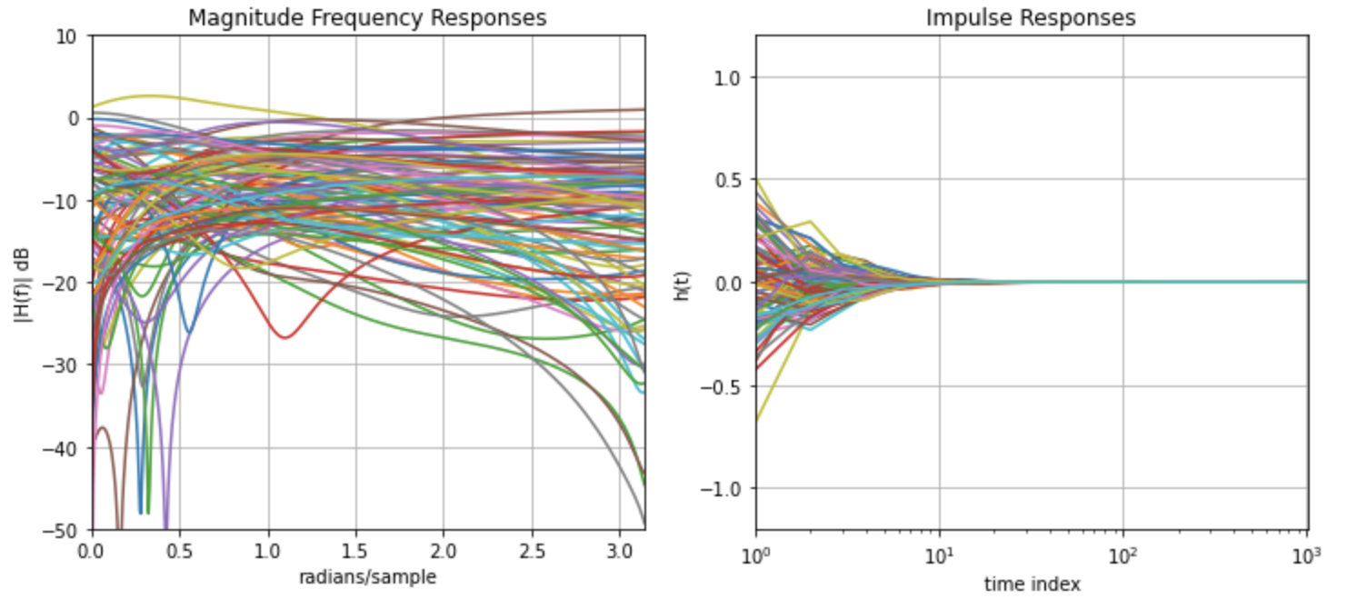
Figure 4: Frequency and impulse responses for a randomly initialized FD RPE MLP with GeLU activations. The curves on the left side are holomorphic, and theory predicts that the curves on the right hand will decay at faster than any exponential rate. They appear to decay approximately exponentially.

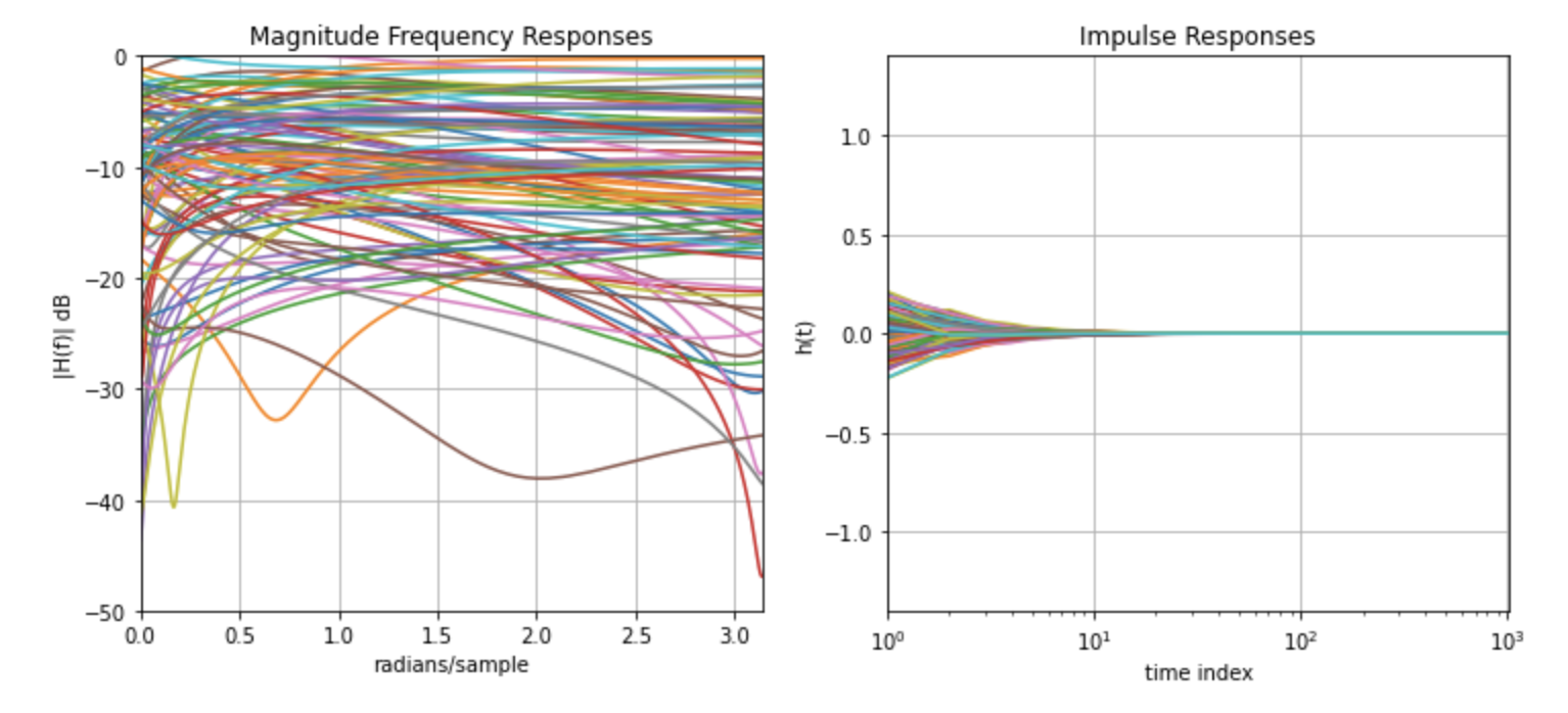
Figure 5: Frequency and impulse response for a randomly initialized FD RPE MLP with SiLU activations. The curves on the left side are $C^{\infty}$, and theory predicts that the curves on the right will decay at faster than any polynomial rate. They appear visually to have ‘almost’ exponential decay.

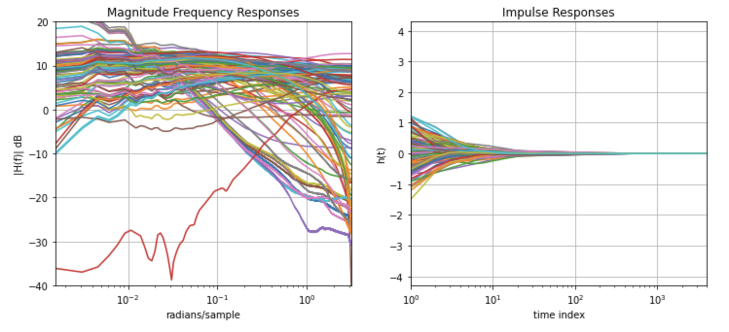
Figure 6: Frequency and impulse responses from an FD RPE MLP with ReLU activations, taken from one layer of a trained FD TNN. The curves on the left are continuous, and theory predicts that the curves on the right will be square summable. They clearly will vanish at infinity, although it is not immediately visually clear at what rate.

Appendix F Experiment Details and Additional Results

F.1 Wikitext-103

F.1.1 Fourier Domain (FD-TNN)

For both causal and bidirectional models we use the default model and training hyperparameters from the TNN repository as the TNN baseline, defined in the first two columns in Qin et al. [2023] Table 13: LM (causal) and Roberta (bidirectional). One small HP discrepancy between the repository and table is the use of 7 decoder layers for the causal LM, which we used for all LM experiments, instead of the 6 they had in their paper. We find that we can reduce the default number of RPE layers from 6 to 3 and improve the speed of the baseline with slight quality improvements. We provide these reproduced perplexity scores for the baseline in parenthesis in Table 1, next to those reported by Qin et al. [2023]. For causal pretraining at a 512 sequence length, FD TNN achieves equivalent perplexity vs inference length as the TNN baseline (see Figure 7a). We achieve between a 5 and 15 % speed up for the causal case, and a nearly 80 % speed up in the best case (6 RPE layers) for the bidirectional case.

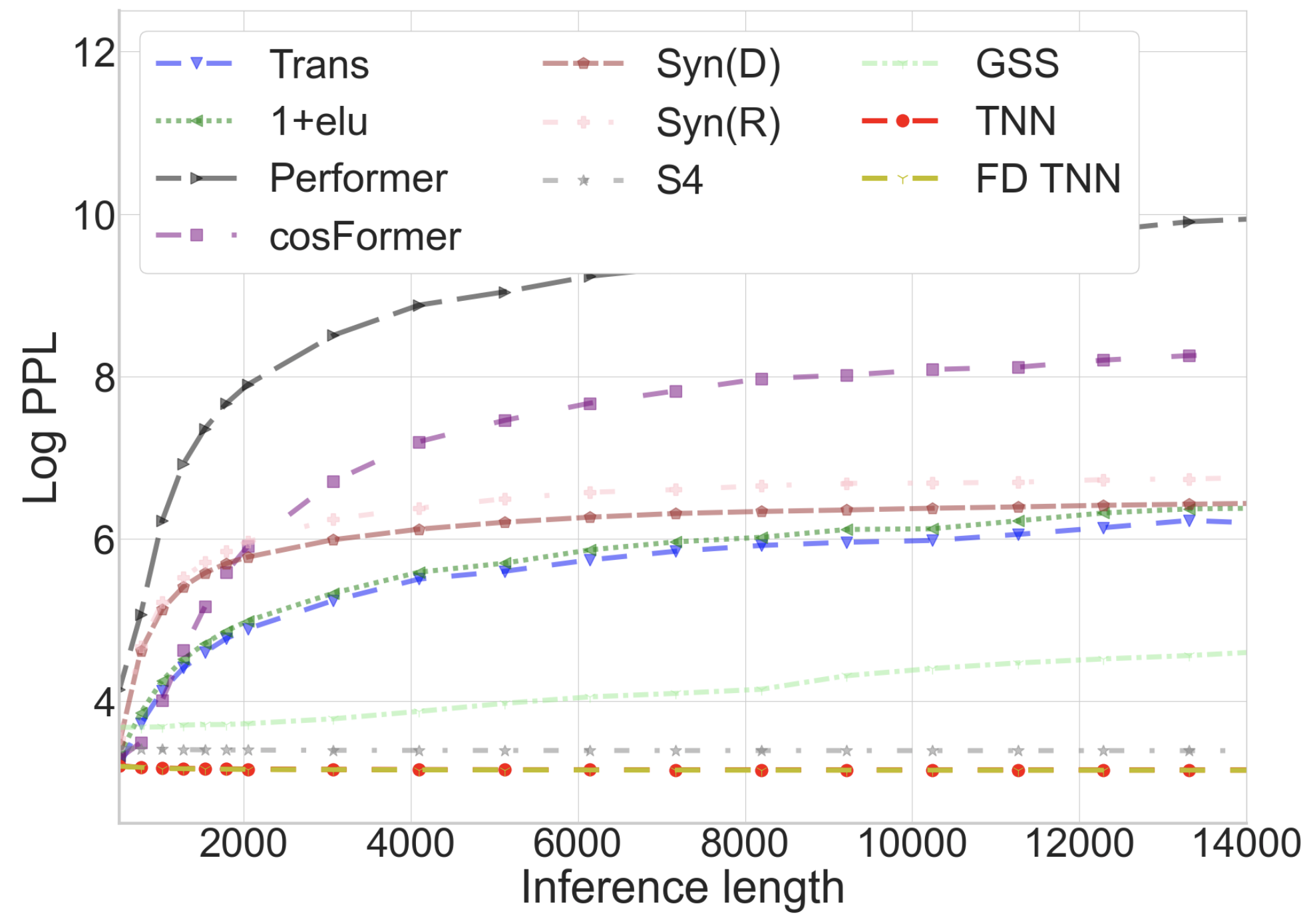
(a) Wikitext-103 Causal Pretraining.

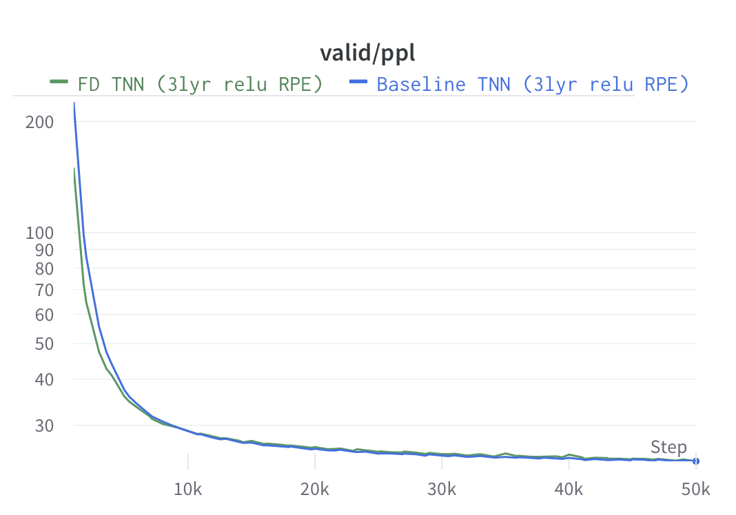
(b) Wikitext-103 Causal Pretraining.

Figure 7: a) In Wikitext-103 causal pretraining, our approach, FD TNN achieves equivalent perplexity vs inference length to TNN. b) Validation Perplexity vs iterations. In the causal setting, FD TNN converges to an equivalent quality at the same rate, but with a 5 to 15% increase in training speed depending on the RPE MLP depth (see Figure 1). For these experiments, we used a learning rate 1e-3 for FD TNN and the default (5e-4) for the baseline.

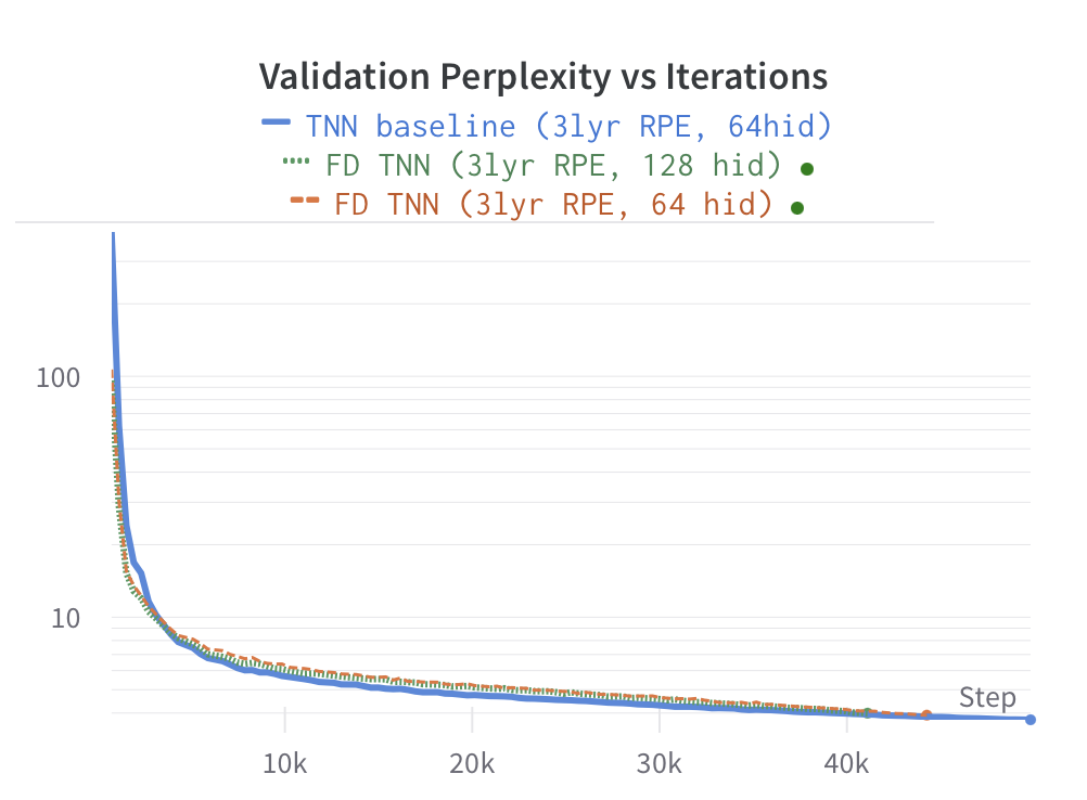
(a) Wikitext-103 Bidirectional Pretraining.

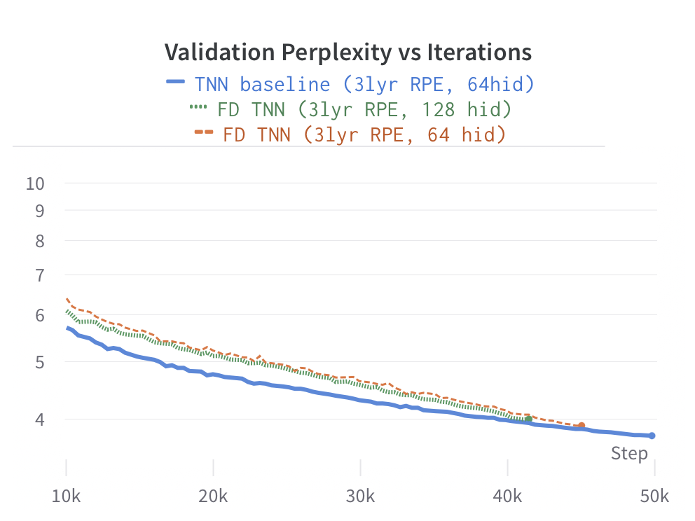
(b) Wikitext-103 Bidirectional Pretraining (close up).

Figure 8: a) In Wikitext-103 bidirectional pretraining, after minimal HP tuning from the default, we observed that FD TNN slightly lags the validation perplexity of the TNN baseline throughout much of the 50k training iterations, but closes this gap during the last 10k iterations. As a result, our 35-80% speed up in iterations/sec (Figure 1(b)) applies to wall clock time assuming one trains for approximately 50k steps. For these results, we used a learning rate of 1e-3 for FD TNN and the default (5e-4) for the baseline.

F.1.2 SKI-TNN

We first train a bidirectional language model using the MLP free SKI-TNN for 50k steps and compare to the same baseline with a 3 layer RPE MLP (which shows improved model quality vs the 6 layer one) for validation perplexity. We see in Figure 9a) that the loss curves are very similar. In 9b), zooming in we see that both validation perplexities are close to $4$, although SKI TNN has slightly higher perplexity.

We then compare the SKI-TNN wall clock time and memory usage for sequence length 512 and 2048 to the 6 layer RPE TNN baseline, which was used in Qin et al. [2023]. Figure 10a) shows approximately 25% speedups compared to the baseline for sequence length 512 and 30% speedups at sequence length 2048. Further, Figure 10b) shows that our approach requires approximately 17% and 42% less memory for sequence lengths 512 and 2048, respectively.

Finally, we analyze the wall clock time and memory allocation for sparse plus low rank (our primary method) vs low rank only SKI. Figure 11 shows the results. We find that the primary bottleneck in both cases is the low rank component, but that for wall clock time the sparse component (1d conv) still adds substantial overhead.

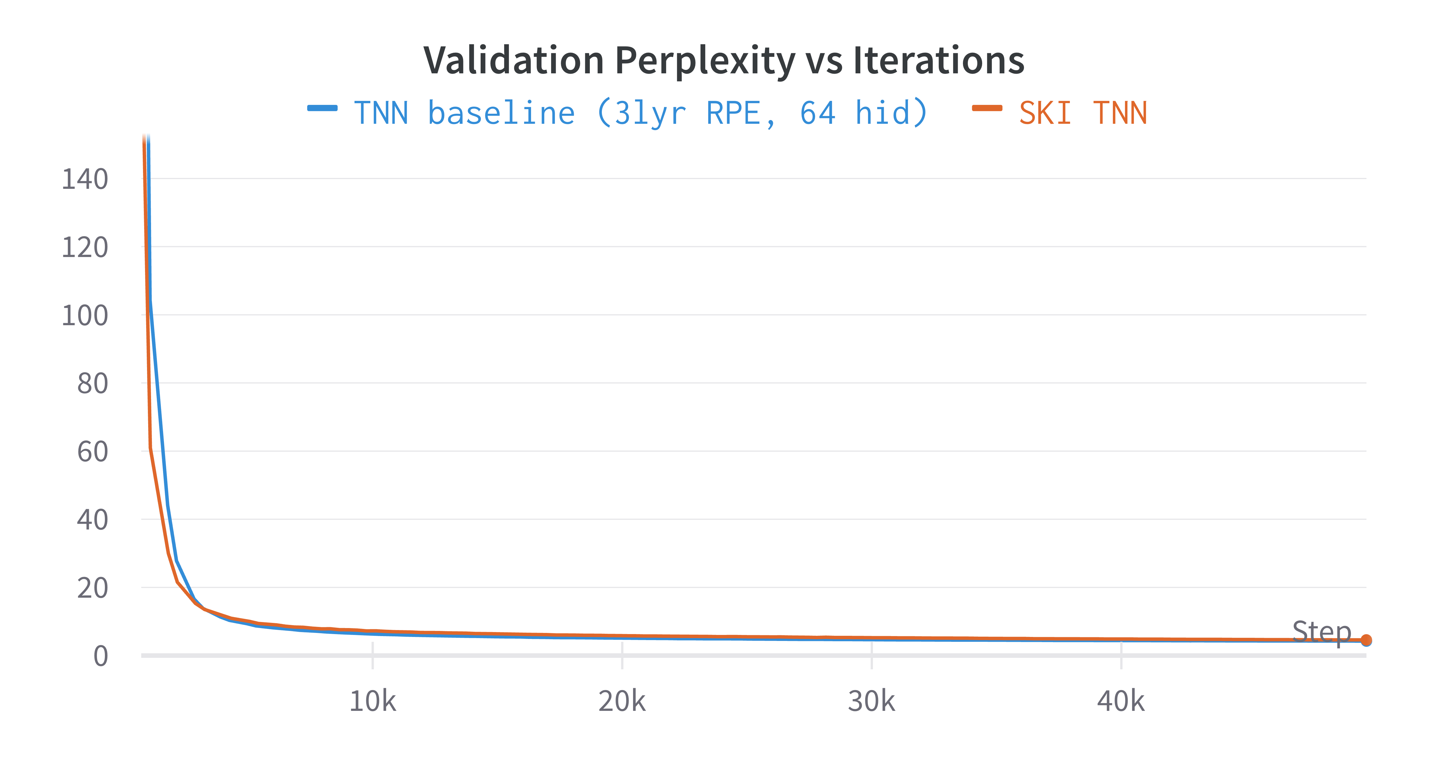
(a) Wikitext-103 Bidirectional Pretraining, SKI.

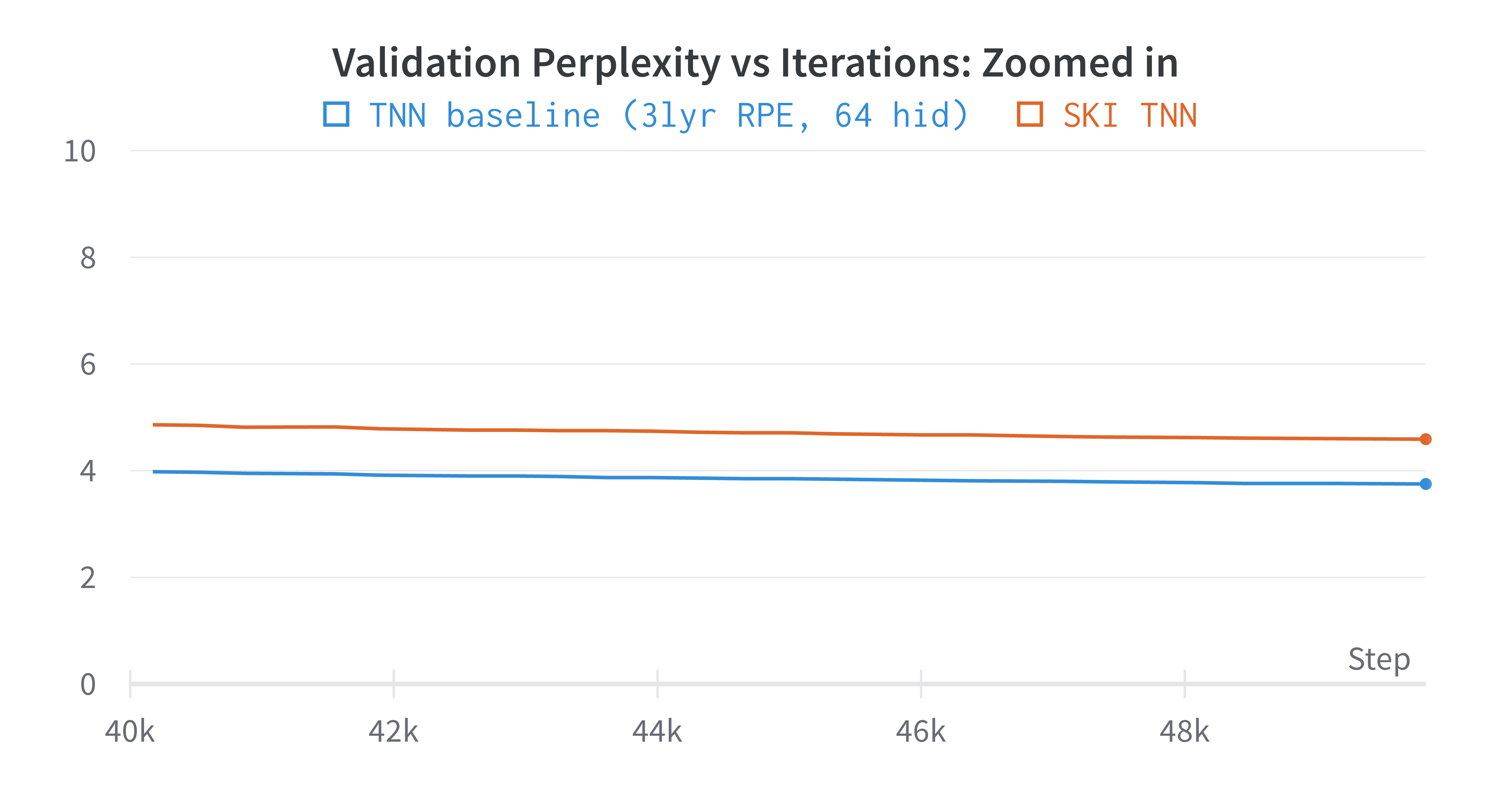
(b) Bidirectional Pretraining, (close up).

Figure 9: a) In Wikitext-103 bidirectional pretraining, using SKI leads to similar validation loss versus the baseline over 50k. b) We zoom in and see that the final validation perplexity is slightly worse, which makes sense as SKI is approximate.

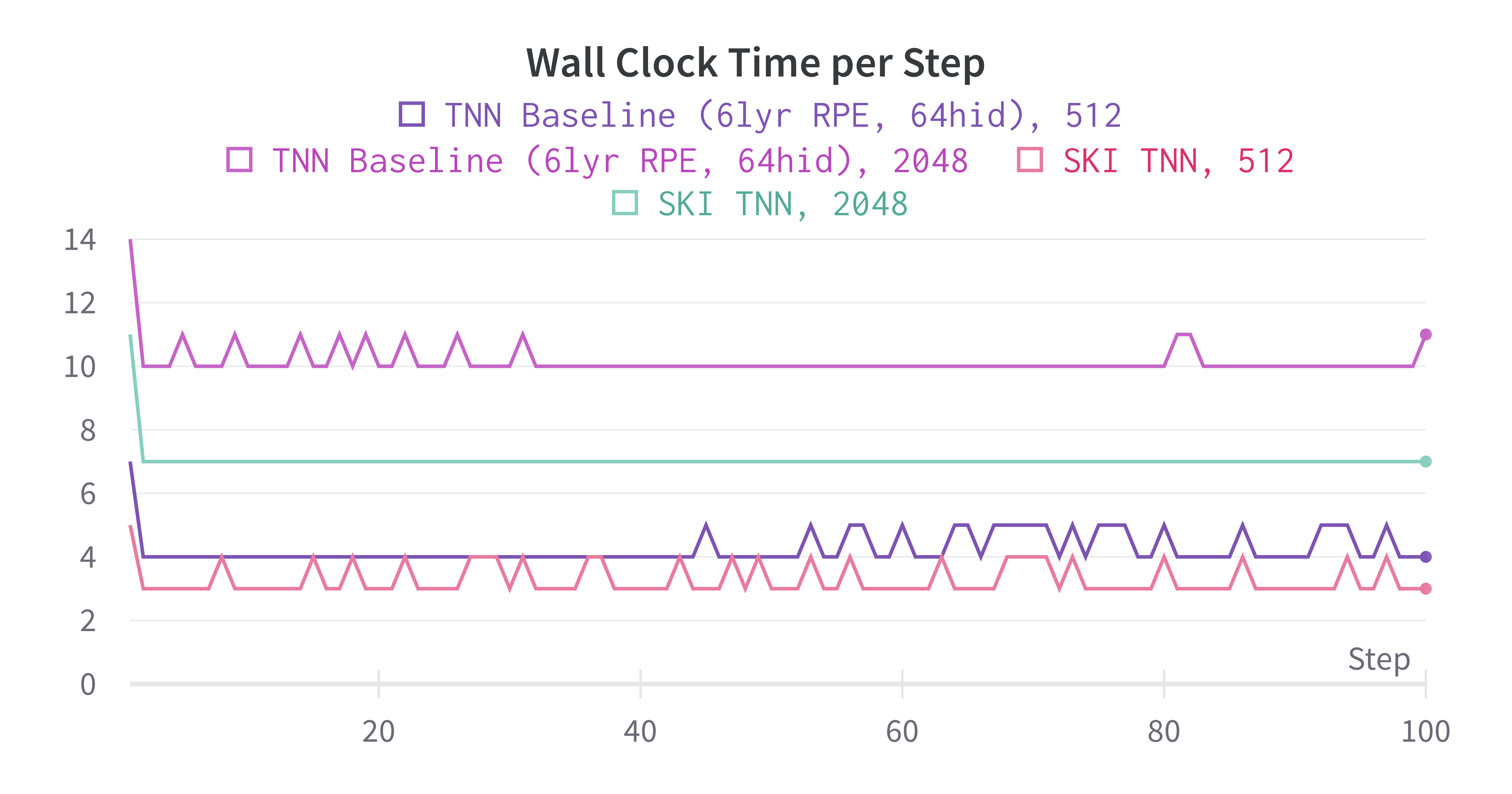
(a) Wall clock time for SKI vs baseline.

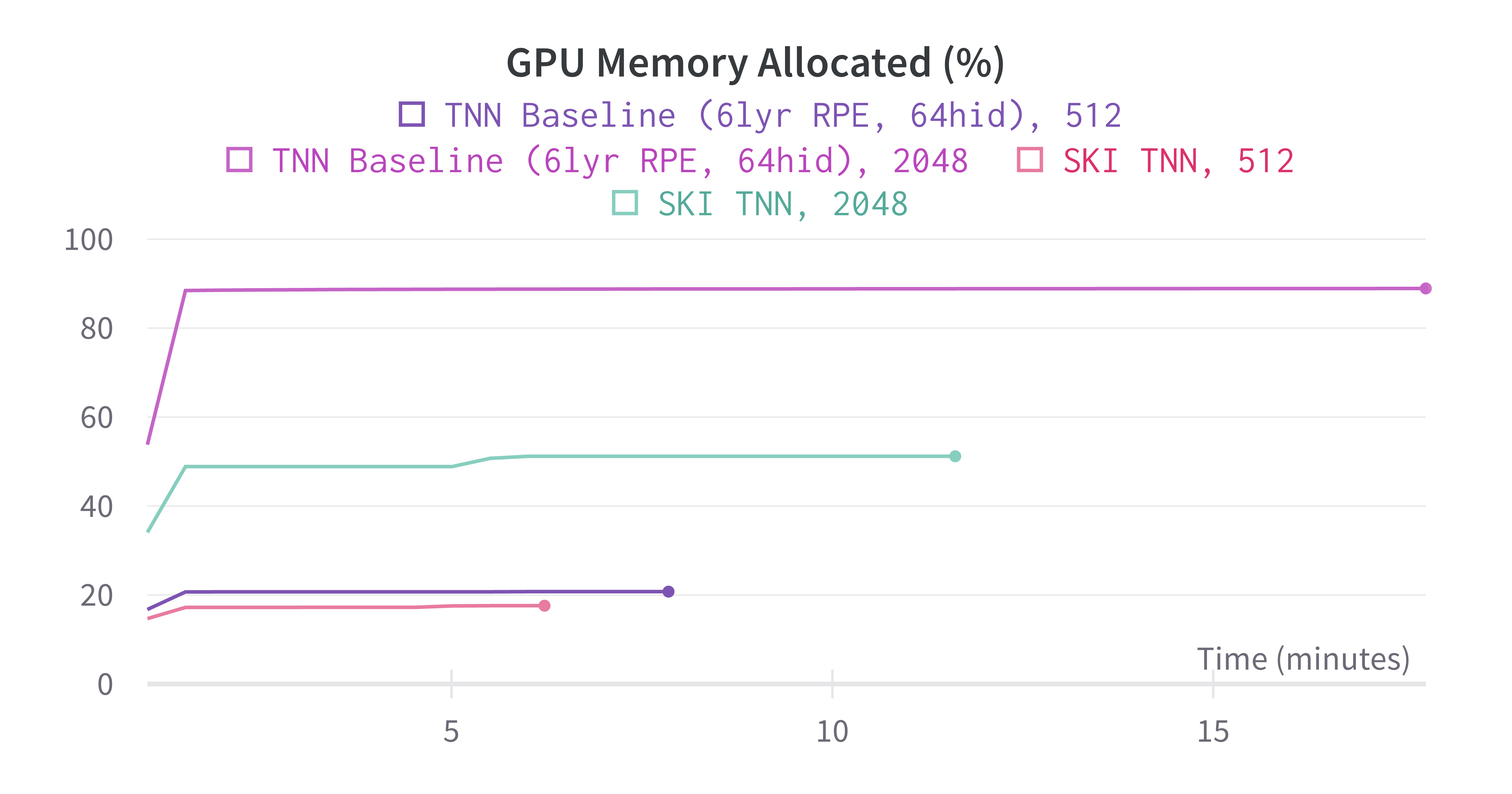
(b) Memory usage for SKI vs baseline.

Figure 10: a) Wall clock time per training step for SKI-TNN at sequence lengths 512 and 2048 vs the baseline with a 6 layer RPE from Qin et al. [2023]. At sequence length 512, our approach has a 25% reduction in time per step in the flat regions. At 2048, our approach has a 30% reduction in time per step. b) GPU memory allocation. At 512, our approach requires approximately 17% less memory. At 2048, our approach requires approximately 42% less memory.

(a) Wall clock time for SKI: low rank only vs sparse plus low rank.

(b) Memory usage for SKI:low rank only vs sparse plus low rank.

Figure 11: a) Wall clock time per training step for SKI-TNN using either the low rank component only or both the sparse and low rank components. We see that the low rank component is the primary bottleneck, but the sparse component (the 1d conv) still adds a substantial amount of time. b) GPU memory allocation for low rank vs sparse plus low rank. Here, nearly all of the memory is due to the low rank component.

References

- Baker (1977) Christopher TH Baker. The numerical treatment of integral equations. Oxford University Press, 1977.
- Brown et al. (2020) Tom Brown, Benjamin Mann, Nick Ryder, Melanie Subbiah, Jared D Kaplan, Prafulla Dhariwal, Arvind Neelakantan, Pranav Shyam, Girish Sastry, Amanda Askell, et al. Language models are few-shot learners. Advances in neural information processing systems, 33:1877–1901, 2020.
- Candes and Plan (2010) Emmanuel J Candes and Yaniv Plan. Matrix completion with noise. Proceedings of the IEEE, 98(6):925–936, 2010.
- Chandrasekaran et al. (2011) Venkat Chandrasekaran, Sujay Sanghavi, Pablo A Parrilo, and Alan S Willsky. Rank-sparsity incoherence for matrix decomposition. SIAM Journal on Optimization, 21(2):572–596, 2011.
- Chandrasekaran et al. (2012) Venkat Chandrasekaran, Pablo A. Parrilo, and Alan S. Willsky. Latent variable graphical model selection via convex optimization. Ann. Stat., 40:1935–1967, 8 2012. ISSN 0090-5364. doi: 10.1214/11-AOS949. URL http://projecteuclid.org/euclid.aos/1351602527.
- Chen et al. (2021) Yifan Chen, Qi Zeng, Heng Ji, and Yun Yang. Skyformer: Remodel self-attention with gaussian kernel and nyström method. Advances in Neural Information Processing Systems, 34:2122–2135, 2021.
- Child et al. (2019) Rewon Child, Scott Gray, Alec Radford, and Ilya Sutskever. Generating long sequences with sparse transformers. arXiv preprint arXiv:1904.10509, 2019.
- Choromanski et al. (2021) Krzysztof Marcin Choromanski, Valerii Likhosherstov, David Dohan, Xingyou Song, Andreea Gane, Tamas Sarlos, Peter Hawkins, Jared Quincy Davis, Afroz Mohiuddin, Lukasz Kaiser, et al. Rethinking Attention with Performers. In International Conference on Learning Representations, 2021.
- Clark et al. (2020) Kevin Clark, Minh-Thang Luong, Quoc V. Le, and Christopher D. Manning. Electra: Pre-training text encoders as discriminators rather than generators. In International Conference on Learning Representations, 2020. URL https://openreview.net/forum?id=r1xMH1BtvB.
- Dao et al. (2022) Tri Dao, Daniel Y Fu, Khaled K Saab, Armin W Thomas, Atri Rudra, and Christopher Ré. Hungry hungry hippos: Towards language modeling with state space models. arXiv preprint arXiv:2212.14052, 2022.
- Fu et al. (2023) Daniel Y Fu, Elliot L Epstein, Eric Nguyen, Armin W Thomas, Michael Zhang, Tri Dao, Atri Rudra, and Christopher Ré. Simple hardware-efficient long convolutions for sequence modeling. arXiv preprint arXiv:2302.06646, 2023.
- Gu et al. (2022) Albert Gu, Karan Goel, and Christopher Re. Efficiently modeling long sequences with structured state spaces. In International Conference on Learning Representations, 2022.
- Heil (2019) Christopher Heil. Introduction to Real Analysis, volume 280. Springer, 2019.
- Hoffmann et al. (2022) Jordan Hoffmann, Sebastian Borgeaud, Arthur Mensch, Elena Buchatskaya, Trevor Cai, Eliza Rutherford, Diego de las Casas, Lisa Anne Hendricks, Johannes Welbl, Aidan Clark, Tom Hennigan, Eric Noland, Katherine Millican, George van den Driessche, Bogdan Damoc, Aurelia Guy, Simon Osindero, Karen Simonyan, Erich Elsen, Oriol Vinyals, Jack William Rae, and Laurent Sifre. An empirical analysis of compute-optimal large language model training. In Alice H. Oh, Alekh Agarwal, Danielle Belgrave, and Kyunghyun Cho, editors, Advances in Neural Information Processing Systems, 2022. URL https://openreview.net/forum?id=iBBcRUlOAPR.
- (15) Mhenni Benghorbal (https://math.stackexchange.com/users/35472/mhenni benghorbal). How to prove error function erf is entire (i.e., analytic everywhere)? Mathematics Stack Exchange, 2017. URL https://math.stackexchange.com/q/203920. URL:https://math.stackexchange.com/q/203920 (version: 2017-04-13).
- Katharopoulos et al. (2020) Angelos Katharopoulos, Apoorv Vyas, Nikolaos Pappas, and François Fleuret. Transformers are RNNs: Fast autoregressive transformers with linear attention. In International Conference on Machine Learning, pages 5156–5165. PMLR, 2020.
- Khalitov et al. (2023) Ruslan Khalitov, Tong Yu, Lei Cheng, and Zhirong Yang. Chordmixer: A scalable neural attention model for sequences with different length. In The Eleventh International Conference on Learning Representations, 2023. URL https://openreview.net/forum?id=E8mzu3JbdR.
- Luo et al. (2021) Shengjie Luo, Shanda Li, Tianle Cai, Di He, Dinglan Peng, Shuxin Zheng, Guolin Ke, Liwei Wang, and Tie-Yan Liu. Stable, fast and accurate: Kernelized attention with relative positional encoding. Advances in Neural Information Processing Systems, 34:22795–22807, 2021.
- Ma et al. (2023) Xuezhe Ma, Chunting Zhou, Xiang Kong, Junxian He, Liangke Gui, Graham Neubig, Jonathan May, and Luke Zettlemoyer. Mega: Moving average equipped gated attention. In The Eleventh International Conference on Learning Representations, 2023. URL https://openreview.net/forum?id=qNLe3iq2El.
- Mei and Moura (2018) Jonathan Mei and José M F Moura. SILVar: Single Index Latent Variable Models. IEEE Transactions on Signal Processing, 66:2790 – 2803, 3 2018.
- Merity et al. (2016) Stephen Merity, Caiming Xiong, James Bradbury, and Richard Socher. Pointer Sentinel Mixture Models. In International Conference on Learning Representations, 2016.
- Nemtsov et al. (2016) Arik Nemtsov, Amir Averbuch, and Alon Schclar. Matrix compression using the Nyström method. Intelligent Data Analysis, 20(5):997–1019, 2016.
- Nyström (1930) Evert J Nyström. Über die praktische auflösung von integralgleichungen mit anwendungen auf randwertaufgaben. Acta Mathematica, 54(1):185–204, 1930.
- Oppenheim and W (2010) Alan V Oppenheim and Schafer R W. Discrete Time Signal Processing. Prentice-Hall, 2010.
- Paszke et al. (2019) Adam Paszke, Sam Gross, Francisco Massa, Adam Lerer, James Bradbury, Gregory Chanan, Trevor Killeen, Zeming Lin, Natalia Gimelshein, Luca Antiga, et al. Pytorch: An imperative style, high-performance deep learning library. Advances in neural information processing systems, 32, 2019.
- Peng et al. (2021) H Peng, N Pappas, D Yogatama, R Schwartz, N Smith, and L Kong. Random Feature Attention. In International Conference on Learning Representations, 2021.
- Poli et al. (2023) Michael Poli, Stefano Massaroli, Eric Nguyen, Daniel Y Fu, Tri Dao, Stephen Baccus, Yoshua Bengio, Stefano Ermon, and Christopher Ré. Hyena Hierarchy: Towards Larger Convolutional Language Models. arXiv preprint arXiv:2302.10866, 2023.
- Proakis and Manolakis (1988) John G Proakis and Dimitris G Manolakis. Introduction to digital signal processing. Prentice Hall Professional Technical Reference, 1988.
- Qin et al. (2023) Zhen Qin, Xiaodong Han, Weixuan Sun, Bowen He, Dong Li, Dongxu Li, Yuchao Dai, Lingpeng Kong, and Yiran Zhong. Toeplitz neural network for sequence modeling. In The Eleventh International Conference on Learning Representations, 2023.
- Rahimi and Recht (2007) Ali Rahimi and Benjamin Recht. Random features for large-scale kernel machines. Advances in neural information processing systems, 20:1177–1184, 2007.
- Recht et al. (2010) Benjamin Recht, Maryam Fazel, and Pablo A Parrilo. Guaranteed minimum-rank solutions of linear matrix equations via nuclear norm minimization. SIAM review, 52(3):471–501, 2010.
- Romero et al. (2022) David W Romero, Anna Kuzina, Erik J Bekkers, Jakub Mikolaj Tomczak, and Mark Hoogendoorn. Ckconv: Continuous kernel convolution for sequential data. In International Conference on Learning Representations, 2022.
- Shazeer (2020) Noam Shazeer. Glu variants improve transformer. arXiv preprint arXiv:2002.05202, 2020.
- Smith et al. (2023) Jimmy T.H. Smith, Andrew Warrington, and Scott Linderman. Simplified state space layers for sequence modeling. In The Eleventh International Conference on Learning Representations, 2023. URL https://openreview.net/forum?id=Ai8Hw3AXqks.
- Tay et al. (2020) Yi Tay, Mostafa Dehghani, Samira Abnar, Yikang Shen, Dara Bahri, Philip Pham, Jinfeng Rao, Liu Yang, Sebastian Ruder, and Donald Metzler. Long Range Arena: A Benchmark for Efficient Transformers. In International Conference on Learning Representations, 2020.
- Tay et al. (2022) Yi Tay, Mostafa Dehghani, Dara Bahri, and Donald Metzler. Efficient transformers: A survey. ACM Computing Surveys, 55(6):1–28, 2022.
- Vaswani et al. (2017) Ashish Vaswani, Noam Shazeer, Niki Parmar, Jakob Uszkoreit, Llion Jones, Aidan N Gomez, Łukasz Kaiser, and Illia Polosukhin. Attention is all you need. Advances in neural information processing systems, 30, 2017.
- Wang et al. (2019) Alex Wang, Amanpreet Singh, Julian Michael, Felix Hill, Omer Levy, and Samuel R Bowman. Glue: A multi-task benchmark and analysis platform for natural language understanding. In International Conference on Learning Representations, 2019.
- Wilson and Nickisch (2015) Andrew Wilson and Hannes Nickisch. Kernel interpolation for scalable structured Gaussian processes (KISS-GP). In International conference on machine learning, pages 1775–1784. PMLR, 2015.
- Wong (2020) Jeffrey Wong. Math 563 lecture notes, polynomial interpolation: the fundamentals, 2020. URL:https://services.math.duke.edu/ jtwong/math563-2020/lectures/Lec1-polyinterp.pdf.
- Xiong et al. (2021) Yunyang Xiong, Zhanpeng Zeng, Rudrasis Chakraborty, Mingxing Tan, Glenn Fung, Yin Li, and Vikas Singh. Nyströmformer: A nyström-based algorithm for approximating self-attention. In Proceedings of the AAAI Conference on Artificial Intelligence, volume 35, pages 14138–14148, 2021.
- Zaheer et al. (2020) Manzil Zaheer, Guru Guruganesh, Kumar Avinava Dubey, Joshua Ainslie, Chris Alberti, Santiago Ontanon, Philip Pham, Anirudh Ravula, Qifan Wang, Li Yang, et al. Big Bird: Transformers for Longer Sequences. Advances in neural information processing systems, 33:17283–17297, 2020.
- Zhang and Yang (2018) Teng Zhang and Yi Yang. Robust PCA by manifold optimization. The Journal of Machine Learning Research, 19(1):3101–3139, 2018.
- Zhou and Tao (2011) Tianyi Zhou and Dacheng Tao. Godec: Randomized low-rank & sparse matrix decomposition in noisy case. In Proceedings of the 28th International Conference on Machine Learning, 2011.