Probing hidden sectors with a muon beam: implication of spin-0 dark matter mediators for muon $(g-2)$ anomaly and validity of the Weiszäcker-Williams approach

Abstract

In addition to vector ($V$) type new particles extensively discussed previously, both CP-even ($S$) and CP-odd ($P$) spin-0 Dark Matter (DM) mediators can couple to muons and be produced in the bremsstrahlung reaction $\mu^{-}+N\rightarrow\mu^{-}+N+S(P)$. Their possible subsequent invisible decay into a pair of Dirac DM particles, $S(P)\to\chi\overline{\chi}$, can be detected in fixed target experiments through missing energy signature. In this paper, we focus on the case of experiments using high-energy muon beams. For this reason, we derive the differential cross-sections involved using the phase space Weiszäcker-Williams approximation and compare them to the exact-tree-level calculations. The formalism derived can be applied in various experiments that could observe muon-spin-0 DM interactions. This can happen in present and future proton beam-dump experiments such as NA62, SHIP, HIKE, and SHADOWS; in muon fixed target experiments as NA64$\mu$, MUoNE and M3; in neutrino experiments using powerful proton beams such as DUNE. In particular, we focus on the NA64$\mu$ experiment case, which uses a 160 GeV muon beam at the CERN Super Proton Synchrotron accelerator. We compute the derived cross-sections, the resulting signal yields and we discuss the experiment projected sensitivity to probe the relic DM parameter space and the $(g-2)_{\mu}$ anomaly favoured region considering $10^{11}$ and $10^{13}$ muons on target.

I Introduction

The Standard Model (SM) cannot explain the origin of dark matter (DM), although it makes up almost $\simeq 85\%$ of the Universe’s matter [1]. The indirect evidence of DM are associated with the rotational velocities of galaxies, the cosmic structure of a large scale, the anisotropy of the cosmic microwave background, and gravity lensing [2, 3, 4]. Nevertheless, the composition of DM continues to be one of the most challenging puzzles for particle physics.

Theoretically, well-motivated scenarios to explain the origin of Dark Matter as a thermal freeze-out relic involve the presence of feebly interacting light scalars from dark sectors (DS) [5, 6]. This framework addresses the origin of DM using a similar mechanism to the weakly interacting massive particles and could imply the existence of sub-GeV spin-0 DM mediators with feebly interaction strength [7].

In addition, the observed low energy experimental anomalies such as the recently confirmed tension of $4.2\sigma$ [8] in the measurement of the muon’s anomalous magnetic moment [9]

$$\Delta a_{\mu}\equiv a_{\mu}^{\rm exp}-a_{\mu}^{\rm th}=(251\pm 59)\cdot 10^{-11},$$ (1)

has also motivated the existence of physics beyond the Standard Model and could be explained in DS framework [10]. We note that recent calculations [11, 12, 13, 14, 15, 16] of the hadronic vacuum polarisation contribution to $(g-2)_{\mu}$ shifts the anomaly to the level of $\Delta a_{\mu}=(183\pm 59)\cdot 10^{-11}$, that corresponds to a significance of $3.1\sigma$ [17] (for recent experimental results from CMD-3 collaboration see e. g. Ref. [18]). In the present paper, we consider the result (1) as a hint of new physics. In particular, a possible solution to that discrepancy involves the introduction of a new weak coupling between the standard matter and a light scalar DM mediator [5, 19, 20]. Other possibility to address the anomaly considers the case of a light vector mediator (see more details in [21, 22]). This study focuses on the computation of the production cross sections of scalar ($S$) and pseudo-scalar ($P$) mediators after a high energy muon scatters off in a target (see e. g. Fig. 1). Our study is particularly relevant to experiments involving high energy muon interactions with a fixed target such as muon experiments NA64$\mu$ at CERN [23, 22] or the proposal $M^{3}$ at Fermilab [19]. Nevertheless, it can also be relevant for i) current and planned proton beam-dump experiments such as NA62 [24], SHIP  [25], HIKE [26], SHADOWS [27], the ILC beam dump [28, 29], ii) muon beam-dump  [30], iii) the MUonE experiment [31] and iv) DUNE [32] aiming also to perform complementary searches to such hidden particles. In this manuscript, we take as an example the NA64$\mu$ experiment at CERN devoted to probe weakly coupled dark sectors with muons.

In the NA64$\mu$ experiment, a 160 GeV muon beam is directed to an electromagnetic calorimeter functioning as an active target, where the spin-0 DM mediators are produced. The resulting particles carry away a portion of the primary muon beam energy. The measurement of the primary muon missing momentum is the key feature of the experimental technique.

In this paper, the production cross-section of spin-0 particles on the reaction $\mu N\to\mu NS(P)$ are derived. In particular, we show that the widely used Weizsäcker-Williams (WW) approach for the spin-0 production reproduces the exact tree level (ETL) cross sections with an accuracy at the level of $\lesssim\mathcal{O}(5\%)$. Furthermore, a novel analytical formula for computing the differential cross-sections in the WW approximation has been obtained in order to perform more accurate and less computationally demanding MC simulations of a dark boson emission. The results have been implemented in the Geant4-based Dark Matter simulation package DMG4 [33, 34, 35]. Additionally, we analyse the differential cross sections with respect to the recoil angles of the muon and spin-0 DM mediators relevant to obtain accurate and realistic signal yields in fixed target experiments.

This paper is organised as follows: In section II, we discuss the typical scenarios for spin-0 DM mediators. In section III, we calculate at ETL the total cross-section for spin-0 mediator production. In section IV, we discuss the differential cross-sections for the angle and energy fraction of the outgoing particles in the WW approach. In section V, we derive novel analytical differential cross-sections for the emitted spin-0 mediator in WW approach. In section VI we compare WW and ETL cross sections. Finally, in section VII, we evaluate the projected sensitivities for NA64$\mu$ experiment in leptophilic scenarios. We summarise our results and conclusions in section VIII.

II A simplified muon-philic model

In this paper, we focus on lepton-specific spin-0 mediators that do not need to couple to neutrinos and assume muon-specific couplings of (pseudo-) scalar boson. The simplified muon-philic spin-$0$ boson Lagrangians can be written for scalar, $S$, and pseudo-scalar, $P$, respectively as follows

$$\mathcal{L}\supset\mathcal{L}_{SM}+\frac{1}{2}(\partial_{\mu}S)^{2}-\frac{1}{2}m_{S}^{2}S^{2}+g_{S}S\overline{\mu}\mu,$$ (2)

$$\mathcal{L}\supset\mathcal{L}_{SM}+\frac{1}{2}(\partial_{\mu}P)^{2}-\frac{1}{2}m_{P}^{2}P^{2}+ig_{P}P\overline{\mu}\gamma_{5}\mu,$$ (3)

where $\mathcal{L}_{SM}$ is the SM Lagrangian, $g_{S(P)}$ is the coupling strength to muons and $m_{S(P)}$ the mass of the mediator. The extension to the Dark Sector can be introduced through the benchmark couplings to Dirac DM fermions

$$\mathcal{L}\supset\overline{\chi}(i\gamma^{\mu}\partial_{\mu}-m_{\chi})\chi+g_{S}^{\chi}S\,\overline{\chi}\chi,$$ (4)

$$\mathcal{L}\supset\overline{\chi}(i\gamma^{\mu}\partial_{\mu}-m_{\chi})\chi+ig_{P}^{\chi}P\,\overline{\chi}\gamma_{5}\chi,$$ (5)

where $m_{\chi}$ is a mass of DM particle, $g_{S}^{\chi}$ and $g_{P}^{\chi}$ are the typical DM couplings to scalar and pseudo-scalar mediators respectively. Moreover, we assume that the invisible decay of $S(P)\to\chi\overline{\chi}$ will be the dominant channel. This means that we focus only on the benchmark regime $m_{S(P)}\gtrsim 2m_{\chi}$ and $g_{S(P)}^{\chi}\gg g_{S(P)}$ in the present study.

We also note that scalar couplings (2) can be originated from flavour specific Lagrangian of higher dimensions in Higgs extended sectors [36] that can be probed by accelerator-based experiments [5, 19, 20]. For pseudo-scalar benchmark couplings (3) we address the reader to Ref. [37], where muon-specific ALPs signatures were studied in detail in the light of atmospheric probes of ALPs using Cerenkov detectors near the Earth’s surface.

The one-loop leading order contributions from scalars to the $(g-2)_{\mu}$ are obtained through the Yukawa-like interaction and are given by [38, 39, 40, 41]

$$\Delta a_{S}=\frac{g_{S}^{2}}{8\pi^{2}}\int_{0}^{1}dx\ \frac{m_{\mu}^{2}(1-x)(1-x^{2})}{m_{\mu}^{2}(1-x)^{2}+m_{S}^{2}x},$$ (6)

where we defined $g_{S}=e\epsilon_{S}$, with $e=\sqrt{4\pi\alpha}$ the electric charge and $\alpha\simeq 1/137$ the fine-structure constant. In the case where $m_{S}/m_{\mu}\rightarrow 0$, $g_{S}=(3.63\pm 0.43)\times 10^{-4}$.

On the other side, the one-loop contribution of the muon-philic pseudo- scalar boson to $\Delta a_{\mu}$ is negative, so the CP-odd spin-0 mediator can not accommodate the explanation of the $(g-2)_{\mu}$ anomaly [37]. For completeness, we refer the reader to [21] for a discussion of the contribution of the vector-boson. In addition, for recent progress on probing leptophilic dark sector see also Refs. [25, 42, 43, 44].

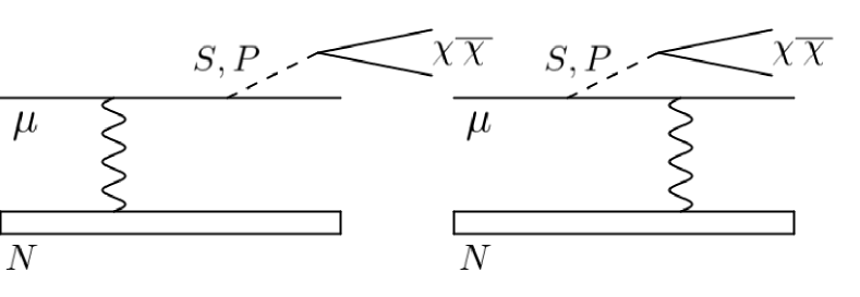
Figure 1: Diagrams describing spin-0 DM mediator production via bremsstrahlung $\mu N\to\mu NS(P)$, followed by invisible decay $S(P)\to\chi\overline{\chi}$.

III The exact tree-level calculation

In the following, we discuss the computations of the exact-tree-level production cross-sections for both, a light scalar and pseudo-scalar muon-philic boson. We follow the notations of [45, 46]. We refer to the kinematic variables of the process $\mu^{-}(p)+N(P_{i})\rightarrow\mu^{-}(p^{\prime})+N(P_{f})+H(k)$ from our previous work [21]. Here we denote via $H=(S,P)$ the general muon-specific CP-even and CP-odd spin-0 boson. Let us recall the definition of the double-differential cross-section [45]

$$\frac{d\sigma}{dx\,d\!\cos\theta_{H}}\Bigr{|}_{ETL}\!\!\!\!\!\!\!=\!\frac{\!\epsilon_{H}^{2}\alpha^{3}|\mathbf{k}|\!E_{\mu}}{|\mathbf{p}||\mathbf{k}\!-\!\mathbf{p}|}\!\!\!\!\int\limits_{t_{\text{min}}}^{t_{\text{max}}}\!\!\!\frac{dt}{t^{2}}G_{2}^{el}(t)\!\!\!\int\limits_{0}^{2\pi}\!\!\frac{d\phi_{q}}{2\pi}\frac{|\mathcal{A}_{2\rightarrow 3}^{H}|^{2}}{8M^{2}},$$ (7)

where $t_{\text{min}}$ and $t_{\text{max}}$ the minimum and maximum momenta transfer and $G_{2}^{el}(t)$ the squared elastic form factor as defined in [45, 47, 21], $\phi_{q}$ is the axial angle of the three momentum transfer to the nucleus $\boldsymbol{q}=\boldsymbol{P}_{i}-\boldsymbol{P}_{f}$ defined in the polar frame in Ref. [45]. The amplitude squared associated to the production of a (pseudo-) scalar boson is calculated using the FeynCalc package [48] embedded in the Wolfram- language-based Mathematica package [49]. With similar kinematics as defined for the vector $V-$boson, we obtain in the case $H=S$

$$|\mathcal{A}_{2\rightarrow 3}^{S}|^{2}=\frac{1}{\tilde{u}^{2}\tilde{s}^{2}}\big{\{}4(4m_{\mu}^{2}-m_{S}^{2})(\mathcal{P}\cdot p^{\prime})^{2}\tilde{s}^{2}$$ (8)

$$-\!4[t(\mathcal{P}\cdot p)^{2}\!-\!2(4m_{\mu}^{2}\!-\!m_{S}^{2}\!+\!t)(\mathcal{P}\!\cdot\!p)(\mathcal{P}\!\cdot\!p^{\prime})\!+\!t(\mathcal{P}\!\cdot\!p^{\prime})^{2}]\tilde{s}\tilde{u}$$

$$+\!4(4m_{\mu}^{2}\!-\!m_{S}^{2}\!)(\mathcal{P}\!\cdot\!p)^{2}\tilde{u}^{2}\!+\!\mathcal{P}^{2}[\tilde{s}\!+\!\tilde{u}]^{2}[(m_{S}^{2}\!-\!4m_{\mu}^{2})t\!+\!\tilde{s}\tilde{u}]\big{\}},$$

as well as for the pseudo-scalar particle, $H=P$,

$$|\mathcal{A}_{2\rightarrow 3}^{P}|^{2}=\frac{1}{\tilde{u}^{2}\tilde{s}^{2}}\big{\{}8(-m_{P}^{2}+t)(\mathcal{P}\cdot p)(\mathcal{P}\cdot p^{\prime})\tilde{s}\tilde{u}$$ (9)

$$-4(\mathcal{P}\cdot p)^{2}\tilde{u}(t\tilde{s}+m_{P}^{2}\tilde{u})$$

$$-4(\mathcal{P}\cdot p^{\prime})^{2}\tilde{s}(t\tilde{u}+m_{P}^{2}\tilde{s})+\mathcal{P}^{2}(\tilde{s}+\tilde{u})^{2}(m_{P}^{2}t+\tilde{s}\tilde{u})\big{\}},$$

for which the relevant Mandelstam variables and dot products read

$$\begin{split}\tilde{s}&=(p^{\prime}+k)^{2}-m_{\mu}^{2}=2(p^{\prime}\cdot k)+m_{H}^{2}\,,\\ \tilde{u}&=(p-k)^{2}-m_{\mu}^{2}=2(p\cdot k)+m_{H}^{2}\,,\end{split}$$ (10)

$$\mathcal{P}^{2}\!=\!4M^{2}\!+\!t(p^{\prime}\!+\!k)^{2}\,,\;(\mathcal{P}\!\cdot\!p)=2ME_{\mu}\!-\!(\tilde{s}\!+\!t)/2\,,$$ (11)

$$\mathcal{P}\cdot p^{\prime}=2M(E_{\mu}-E_{H})+(\tilde{u}-t)/2\,,$$ (12)

with $\mathcal{P}_{\mu}=(P_{i}+P_{f})_{\mu}$, $P_{i}=(M,0)$ being the nucleus four-momentum in the laboratory frame, $P_{f}=(P_{f}^{0},\mathbf{P}_{f})$ is its outgoing momentum. The resulting squared matrix elements Eqs. (8) and (9) coincide with those given in Refs. [45] and [47], implying replacement of the electron with muon, i.e. $m_{e}\to m_{\mu}$.

IV The WW approximations for the (pseudo-)scalar emission cross-sections

In this section, we use the Weizsäcker-Williams (WW) approximation to compute the double-differential production cross-sections for $H$, assuming that the energy of the incoming muon is much larger than both $m_{\mu}$ and $m_{H}$. In this approach, the flux of virtual photons from the moving charged particles can be treated as a plane wave and approximated by real photons.

We follow the same procedure as the one described in [21]. In particular, for the choice of $(x,\theta_{H})$ and $(y,\psi_{\mu})$ variables, the WW-approximated quantities read respectively

$$\frac{d\sigma^{H}_{2\to 3}}{dxd\cos\theta_{H}}\Bigr{|}_{WW}\!\simeq\!\frac{\alpha\chi}{\pi(\!1\!-\!x\!)}E_{\mu}^{2}x\beta_{H}\frac{d\sigma^{H}_{2\to 2}}{d(pk)}\Bigr{|}_{t=t_{\text{min}}},$$ (13)

$$\frac{d\sigma^{H}_{2\to 3}}{dyd\cos\psi_{\mu}}\Bigr{|}_{WW}\simeq\frac{\alpha\chi}{\pi(\!1\!-\!y\!)}E_{\mu}^{2}y\beta_{\mu^{\prime}}\frac{d\sigma^{H}_{2\to 2}}{d(pk)}\Bigr{|}_{t=t_{\text{min}}},$$ (14)

where $\beta_{H}=(1-m_{H}^{2}/(xE_{\mu})^{2})^{1/2}$ and $x=E_{H}/E_{\mu}$ are the typical velocity of the produced hidden boson and its energy fraction respectively, $\beta_{\mu}=(1-m_{\mu}^{2}/(yE_{\mu})^{2})^{1/2}$ and $y=E_{\mu^{\prime}}/E_{\mu}$ are the typical velocity of the recoil muon and its energy fraction respectively, $\psi_{\mu}$ and $\theta_{H}$ are the recoil angles of outgoing muon and the $H$-boson respectively. The expression of the photon flux $\chi$ is given by (31) in Sec. V below. The cross-section of the process $\mu\gamma\to\mu H$ has the following form

$$\frac{d\sigma_{2\to 2}^{H}}{d(pk)}=\epsilon^{2}_{H}\alpha^{2}\frac{2\pi}{\tilde{s}^{2}}\left|\mathcal{A}^{H}_{2\to 2}\right|^{2},$$ (15)

where the squared amplitudes read

$$\left|\mathcal{A}^{S}_{2\to 2}\right|^{2}\!\!\!=\!2(m_{S}^{2}\!-\!4m_{\mu}^{2})\!\!\left[\!\!\left(\!\frac{\tilde{s}\!+\!\tilde{u}}{\tilde{s}\tilde{u}}\!\right)^{2}\!\!\!m_{\mu}^{2}\!-\!\frac{t_{2}}{\tilde{s}\tilde{u}}\!\right]\!\!-\!\frac{(\tilde{s}\!+\!\tilde{u})^{2}}{\tilde{s}\tilde{u}}\!,$$ (16)

$$\left|\mathcal{A}^{P}_{2\to 2}\right|^{2}=2m_{P}^{2}\left[\left(\frac{\tilde{s}+\tilde{u}}{\tilde{s}\tilde{u}}\right)^{2}m_{\mu}^{2}\!-\!\frac{t_{2}}{\tilde{s}\tilde{u}}\!\right]\!-\!\frac{(\tilde{s}+\tilde{u})^{2}}{\tilde{s}\tilde{u}}.$$ (17)

We note that for the $(x,\theta_{H})$ - plane one has the following expressions for the Mandelstam variables

$$\tilde{s}\simeq U/(1-x),\quad U=E_{\mu}^{2}\theta_{H}^{2}x+m_{H}^{2}(1-x)/x+m_{\mu}^{2}x,$$ (18)

$$\tilde{u}\simeq-U,\quad t_{2}=-xU/(1-x)+m_{H}^{2}.$$ (19)

On the other hand, for the $(y,\psi_{\mu})$ - plane the Mandelstam variables read

$$\tilde{s}\simeq\tilde{t}/(1-y),\quad\tilde{u}\simeq-y\tilde{t}/(1-y),\quad\tilde{t}\simeq m_{H}^{2}-t_{2},$$ (20)

$$t_{2}\simeq-[E_{\mu}^{2}\psi_{\mu}^{2}y+m_{\mu}^{2}(1-y)/y+m_{\mu}^{2}y]+m_{\mu}^{2}.$$ (21)

Let us also remark on the typical energy fractions of the outgoing muon and $H$ boson in the process $\mu N\to\mu NH$ for certain benchmark kinematics. The lowest possible energy of the produced $H$-boson implies that $x_{\text{min}}\simeq m_{H}/E_{\mu}\lesssim x$, i. e. in this case the spin-0 particle is produced with zero three-momentum, $|\mathbf{k}|=0$. This means also that almost all energy of the initial muon is transferred to the outgoing muon, which leads to the typical bound $y\lesssim y_{\text{max}}\simeq 1-m_{H}/E_{\mu}$. On the other hand, if the initial muon transfers its maximal energy to spin-0 boson, then we get $y\gtrsim y_{\text{min}}\simeq m_{\mu}/E_{\mu}$ and $x\lesssim x_{\text{max}}\simeq 1-m_{\mu}/E_{\mu}$.

V Analytical integration of the WW approximation over the angle $\theta_{H}$

In the WW approach, the lower bound of the flux integral $t_{\text{min}}$ depends on both the fractional energy $x$ and the emitted angle $\theta_{H}$ of the boson mediator. Although WW provides more accurate results than its improved approach (IWW), the integration of the double-differential cross-section is still computationally expensive, to sample a sufficiently large number of MC events [33]. In this work, we perform an explicit integration over $\theta_{H}$ to obtain an analytical expression for $d\sigma^{H}_{2\rightarrow 3}/dx$. We emphasize that this result can also be expanded to the light $V$ vector boson case.

The formula for the differential cross-section can be rewritten in the following form

$$\frac{d\sigma^{H}_{2\to 3}}{dx}\Bigr{|}_{WW}\!\!\!=\!\epsilon_{H}^{2}\alpha^{3}\sqrt{x^{2}\!-\!\frac{m_{H}^{2}}{E_{\mu}^{2}}}\!\!\frac{1\!-\!x}{x}\!\!\!\int\limits_{u_{\text{min}}}^{u_{\text{max}}}\!\!\!du\frac{\left|\mathcal{A}_{2\rightarrow 2}^{H}\right|^{2}\!\!\chi}{u^{2}},$$ (22)

where the limits of integration over the Mandelstam variable are:

$$u_{\text{max}}=-m_{H}^{2}(1-x)/x-m_{\mu}^{2}x,$$ (23)

$$u_{\text{min}}=-xE_{\mu}^{2}(\theta^{\text{max}}_{H})^{2}-m_{H}^{2}(1-x)/x-m_{\mu}^{2}x,$$ (24)

where $\theta_{H}^{\text{max}}$ is the typical maximal angle between the initial muon and the emission momentum of the $H$ boson. Numerical analysis show (see e. g. Sec. VI below) that for the ultra-relativistic muons expected at NA64$\mu$ one can set $\theta_{H}^{\text{max}}\simeq 0.1$. It is worth noticing that in Eq. (22) we imply $d\cos\theta_{H}\simeq du/(2xE_{\mu}^{2})$ in order to introduce a new variable of the integration $u$ instead of $\cos\theta_{H}$. The transition amplitude squared then reads

$$\left|\mathcal{A}_{2\rightarrow 2}^{H}\right|^{2}(x,u)=C^{H}_{1}+C^{H}_{2}\frac{1}{u}+C^{H}_{3}\frac{1}{u^{2}},$$ (25)

where the coefficients $C_{i}^{H}$ are

$$C^{S}_{1}=C^{P}_{1}=\frac{x^{2}}{1-x},\,C^{S}_{2}=2\left(m_{S}^{2}-4m_{\mu}^{2}\right)x,$$ (26)

$$C^{P}_{2}=2m_{P}^{2}x,\,C^{P}_{3}=2m_{P}^{2}\left(m_{P}^{2}(1-x)+m_{\mu}^{2}x^{2}\right),$$ (27)

$$C^{S}_{3}=2\left(m_{S}^{2}-4m_{\mu}^{2}\right)\left(m_{S}^{2}(1-x)+m_{\mu}^{2}x^{2}\right).$$ (28)

For completeness, we also derive the coefficients for the vector boson emission. In particular, for the case of $H=V$ these quantities read explicitly in the following form

$$C^{V}_{1}=2\frac{(2-2x+x^{2})}{1-x},\quad C^{V}_{2}=4\left(m_{V}^{2}+2m_{\mu}^{2}\right)x,$$ (29)

$$C^{V}_{3}=4\left(m_{V}^{2}+2m_{\mu}^{2}\right)\left(m_{V}^{2}(1-x)+m_{\mu}^{2}x^{2}\right).$$ (30)

The flux of virtual photons $\chi$ in the Weizsacker-Williams approximation can be expressed via the typical elastic atomic form-factor in the following form

$$\chi=Z^{2}\!\!\int\limits_{t_{\text{min}}}^{t_{\text{max}}}\frac{t-t_{\text{min}}}{t^{2}}\left(\frac{t}{t_{a}+t}\right)^{2}\!\!\left(\frac{t_{d}}{t_{d}+t}\right)^{2}\!\!dt=C^{\chi}_{1}\\ +C^{\chi}_{2}u^{2}\!+\!C^{\chi}_{3}\!\ln{\left(\!\frac{u^{2}g^{2}\!+\!t_{d}}{u^{2}g^{2}\!+\!t_{a}}\!\right)}\!+\!C^{\chi}_{4}u^{2}\ln{\!\left(\!\frac{u^{2}g^{2}\!+\!t_{d}}{u^{2}g^{2}\!+\!t_{a}}\!\right)},$$ (31)

where $Z=82$ is the atomic number of the lead target of NA64$\mu$, $\sqrt{t_{a}}=1/R_{a}$ is a momentum transfer associated with nucleus Coulomb field screening due to the atomic electrons, with $R_{a}$ being a typical magnitude of the atomic radius $R_{a}=111Z^{-1/3}/m_{e}$, $\sqrt{t_{d}}=1/R_{n}$ is the typical momentum associated with nuclear radius $R_{n}$, such that $R_{n}\simeq 1/\sqrt{d}$ and $d=0.164A^{-2/3}\text{GeV}^{2}$, $A=207$ is the atomic mass number of the lead target, $t_{\text{min}}=g^{2}u^{2}$ is minimal transfer momentum, here we denote $g=1/(2E_{\mu}(1-x))$ for simplicity. Typically the maximal transfer momentum $t_{\text{max}}$ is chosen to be $t_{\text{max}}=m_{\mu}^{2}+m_{H}^{2}$ in [45, 47], however, the numerical calculations reveal that $t_{\text{max}}$ can be set as large as $t_{\text{max}}\gtrsim t_{d}$ in order to achieve a better accuracy for WW approach. The coefficients $C_{1}^{\chi},C_{2}^{\chi},C_{a}^{\chi}$ and $C_{4}^{\chi}$ in (31) are collected in Appendix A.

By substituting Eqs. (31) and (25) into the differential cross section (22) one can obtain the following expression:

$$\left(\frac{d\sigma}{dx}\right)_{WW}\!\!\!\!\!=\!\epsilon_{H}^{2}\alpha^{3}\!\!\sqrt{x^{2}\!-\!\frac{m_{H}^{2}}{E_{\mu}^{2}}}\frac{1\!-\!x}{x}\!\!\!\int\limits_{u_{\text{min}}}^{u_{\text{max}}}\!\!\!\left\{C^{H}_{1}C^{\chi}_{2}\!+\!\frac{C^{H}_{2}C^{\chi}_{2}}{u}\right.\\ +\frac{C^{H}_{1}C^{\chi}_{1}+C^{H}_{3}C^{\chi}_{2}}{u^{2}}+\frac{C^{H}_{2}C^{\chi}_{1}}{u^{3}}+\frac{C^{H}_{3}C^{\chi}_{1}}{u^{4}}+\\ +\left.\left[C^{H}_{1}C^{\chi}_{4}+\frac{C^{H}_{2}C^{\chi}_{4}}{u}+\frac{C^{H}_{1}C^{\chi}_{3}+C^{H}_{3}C^{\chi}_{4}}{u^{2}}+\right.\right.\\ \left.\left.\frac{C^{H}_{2}C^{\chi}_{3}}{u^{3}}+\frac{C^{H}_{3}C^{\chi}_{3}}{u^{4}}\right]\ln{\left(\frac{u^{2}g^{2}+t_{d}}{u^{2}g^{2}+t_{a}}\right)}\right\}du.$$ (32)

The differential cross section with respect to $x$, can be represented as the the sum of six typical terms

$$\left(\!\frac{d\sigma}{dx}\!\right)_{WW}\!\!\!\!\!\!=\!\epsilon_{H}^{2}\alpha^{3}\!\!\sqrt{\!x^{2}\!-\!\frac{m_{H}^{2}}{E_{\mu}^{2}}}\frac{1\!-\!x}{x}\sum\limits_{i=1}^{6}\Delta I^{H}_{i}(x,u),$$ (33)

where $\Delta I^{H}_{i}(x,u)=I^{H}_{i}(x,u_{\text{max}})-I^{H}_{i}(x,u_{\text{min}})$. The functions $I^{H}_{i}(x,u)$ are described in Appendix A. Alternatively, one can also exploit the state-of-the-art MadGraph [50] or CalcHEP [51] packages with appropriate atomic form-factor implementation [20, 52, 43, 53, 54, 55, 56]. That analysis, however, is beyond the scope of the present paper.

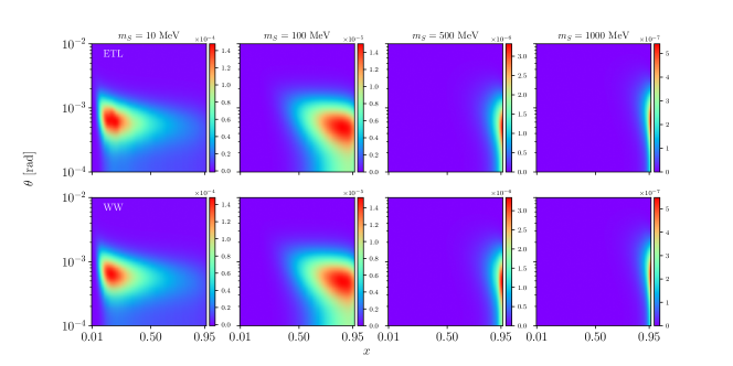
Figure 2: Top: double-differential cross-section at ETL in the $(x,\theta_{S})$ space. The expression of Eq. (7) is integrated using both the angular parametrisation from [57] and MC integration [58]. Bottom: double-differential cross-section in the WW approach for the $(x,\theta_{S})$ variables (see Eq. (13) with an amplitude squared as defined in Eq. (16)). The mass range spans from 10 MeV to 1 GeV. The mixing strength is $\epsilon_{S}=10^{-4}$.

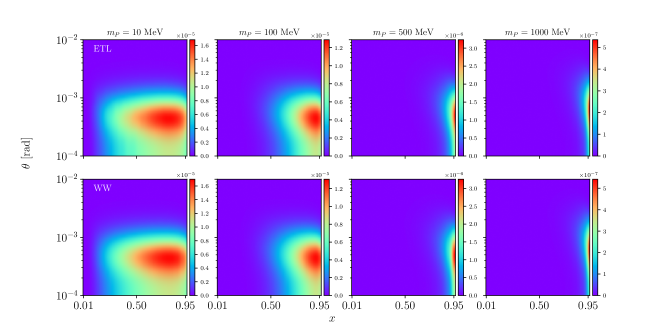
Figure 3: The same as in Fig. 2 but for pseudo-scalar field $P$.

VI Numerical integration of the cross-sections

The comparison between the expression for $d\sigma/dxd\cos\theta_{H}$ at ETL and in the WW approximation is shown for both scalar and pseudo-scalar mediators in Figs. 2 and 3. The $H$ mass spans from 10 MeV to 1 GeV. Following the nominal beam energy of the NA64$\mu$ experiment, the initial state muon energy is set to $E_{\mu}=160\,\leavevmode\nobreak\ \mbox{GeV}$. The integration over $(t,\phi_{q})$ in Eq. (7) is performed using the parametrisation of [57] to integrate out $\phi_{q}$. The integral over $t$ is computed numerically through Monte Carlo integration [58]. Only the region of phase space $(x,\theta_{H})$ where the double-differential cross-section contributes more is shown. Both the complete calculation (ETL) and the WW results have the double differential cross-section peak at the same order of magnitude. Additionally, from both Fig. 2 and 3 it can be seen that $\theta_{H}$ is constant around $\sim 5\times 10^{-4}$ as expected from the typical emission angle $\sim m_{\mu}/E_{\mu}$, which is independent of $m_{H}$. To perform the comparison between the ETL and WW approximated results, Eq. (7) is integrated over $\theta$ and compared to the expression in Eq. (33). The results in the case $H=S$ and $H=P$ are shown respectively in Fig. 4 and Fig. 5. In both cases the integrated differential cross-section relative error with respect to the exact calculation is below $\lesssim\mathcal{O}(5\%)$ for the full mass range.

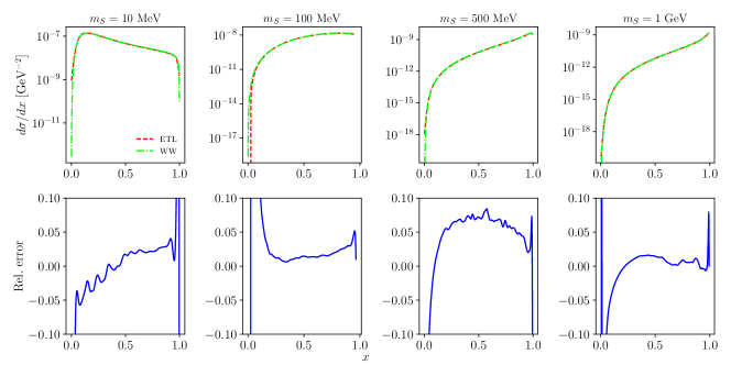
Figure 4: Top: single-differential scalar mediator cross-sections as a function of $x$ in the ETL (red dashed line) and WW approximation (green dashed line) regime for different mass values. The exact approach (ETL) results are obtained numerically through integration by quadrature of the results of Fig. 2. Bottom: relative error, $(\mathcal{O}_{WW}-\mathcal{O}_{ETL})/\mathcal{O}_{ETL}$, between the WW and ETL expressions defined respectively in Eqs. (7) and (33). The mixing strength is $\epsilon_{S}=10^{-4}$.

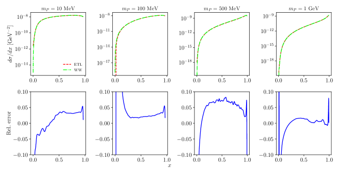
Figure 5: The same as in Fig. 4 but for pseudo-scalar mediator $P$.

However, on the boundaries of the fractional energy domain, $x\rightarrow x_{\text{min}}\ll 1$ and $x\rightarrow x_{\text{max}}\simeq 1$, the relative error can be as large as $\gtrsim\mathcal{O}(5\%)$. After the numerical integration of the differential cross-section, this effect is negligible. Therefore, the yields of the produced spin-0 bosons can be calculated accurately in WW approach [21].

For completeness, the single differential cross-sections with respect to the outgoing muon fractional energy, $y$, and emission angle, $\psi$, are integrated according to Eq. (14). The results are illustrated in Figs. 6 and 7. Similarly as in the result for the integration over $x$, the integrated differential cross-section relative error is of the order $\lesssim\mathcal{O}(5\%)$.

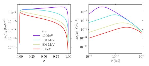
Figure 6: Single-differential scalar mediator cross-sections in WW approximation regime for different mass values (from the top to the bottom line the masses are 10, 100, 500 and 1000 MeV). The mixing strength is $\epsilon_{S}=10^{-4}$. Left: single-differential cross-section as a function of the outgoing muon fractional energy. Right: single-differential cross-section as a function of the outgoing muon angle.

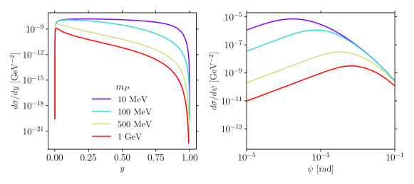
Figure 7: The same as in Fig. 6 but for pseudo-scalar mediator $P$.

VII Projected sensitivities to the mixing strength

The typical estimate of the sensitivity of a given experiment can be computed following the yield formula [46]

$$N_{H}=N_{\text{MOT}}\frac{\rho\mathcal{N}_{A}}{A}\sum_{i}\sigma_{H}(E_{i})\Delta L_{i},$$ (34)

where $\rho$ and $A$ are respectively the target density and its atomic weight, $E_{i}$ the energy of the muon at the $i-$th step-length $\Delta L_{i}$ in the target and $N_{\text{MOT}}$ the number of muons on target. We recall that NA64$\mu$ target is a lead-scintillator sandwich electromagnetic calorimeter of $40$ radiation lengths $(40X_{0})$ [22]. However, for a realistic sensitivity study of one’s experiment to New Physics models, including particles propagation through the detectors, the differential cross-sections for the production of light muon-philic mediators are implemented using the interface provided by the fully GEANT4 [59] compatible DMG4 package. In Fig. 8 the production yields for both cases $H=S$ and $H=P$ as obtained through a realistic GEANT4 simulation of the NA64$\mu$ detectors are shown. The number of signal events $N_{H}$ are given in the scenario where $\epsilon_{H}=10^{-4}$. For completeness, the yield for the vector case ($H=V$), for which the similar calculations and implementation were performed previously, is plotted.

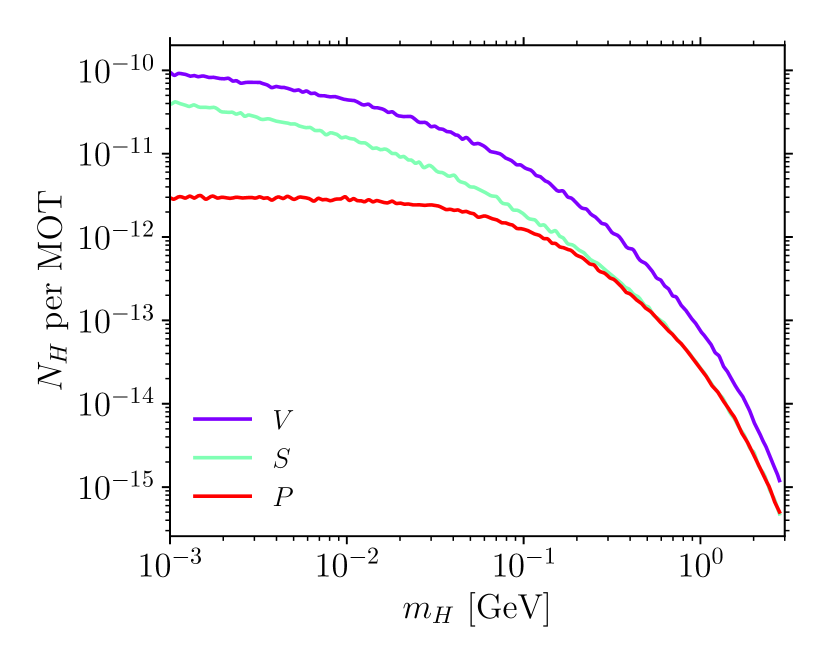
Figure 8: Number of light mediators, $N_{H}$, per muons on target (MOT) as obtained through a full GEANT4 simulation of the NA64$\mu$ target using the DMG4 package ($\epsilon_{H}=10^{-4}$ is considered in this case). For completeness, in addition to the scalar $(S)$ and pseudo-scalar $(P)$ mediators is also shown the vector $(V)$ case.

The sensitivity of the experiment in the case where $H=S$ and $H=P$ is shown in Fig. 9 in the invisible scenario, $S\rightarrow\mbox{invis}.$, in the target parameter space $(m_{H},\ g_{H})$. Eq. (33) is considered, i.e. the WW regime. The limits are calculated at 90% C. L., requiring $N_{H}\gtrsim 2.3$, and assuming 100% efficiency and no background. In the chosen mass range, both sensitivities for the case $H=S$ and $H=P$ yield similar reach as Eqs. (16) and (17) only differ by the typical factors $m_{S}^{2}-4m_{\mu}^{2}$ and $m_{P}^{2}$.

NA64$\mu$ projected sensitivity for $10^{13}$ MOT can completely probe the New Physics contribution to the $(g-2)_{\mu}$ anomaly for a muon-philic scalar mediator for masses below 3 GeV. The DM relic predictions have been obtained in [5]. The ¨kink¨ present in the DM relic curves arises as at $m_{S}=2m_{\mu}$ a new annihilation channel to muons is kinematically accessible. For a similar mass range and MOT, the target parameter space for thermal relic DM with a scalar mediator is fully accessible in the scenario where $g_{S}^{\chi}=1$ and $m_{S}=3m_{\chi}$. Because of the similar behaviour of the cross- sections at masses above the muon mass ($m_{S}\gtrsim m_{\mu}$), the previous statement is also valid in the case of a pseudo-scalar mediator, $H=P$. In the near-resonant scenario for which $m_{S}\simeq 2.1m_{\chi}$, only the portion of parameter space with $m_{H}\lesssim\mathcal{O}(m_{\mu})$ is accessible. Note that for completeness projected sensitivities from both $M^{3}$ phases I and II are shown for $10^{10}$ MOT and $10^{13}$ MOT respectively given the phase-space values provided in [19]. Additionally, the ATLAS-HL [60] and FASER$\nu$(2) [56] expected limits are shown.

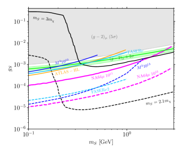
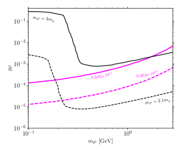
Figure 9: Projected sensitivity in the $(m_{H},g_{\mu})$ phase space obtained through numerical integration of Eq. (33) through [58] for $10^{11}$ (plain magenta line) and $10^{13}$ (dashed magenta line) MOT. The limits are calculated at 90% C.L. Left: scalar ($S$) case. Are also shown the $(g-2)_{\mu}\pm 2\sigma$ band following Eq. (6) and the thermal freeze-out target as computed in [5] for the scenario $g_{\chi}=1$ both with $m_{S}=3m_{\chi}$ and $m_{S}\simeq 2.1m_{\chi}$. The $M^{3}$ experiment phases 1 and 2 (plain and dashed blue lines) are shown for completeness [19] together with the ATLAS HL-LHC analysis at $\mathcal{L}_{\text{LHC}}=3$ ab^-1 [60] (orange line) and the FASER$\nu$ projected sensitivity at $\mathcal{L}_{\text{LHC}}=250$ fb^-1 (light blue line) and $\mathcal{L}_{\text{LHC}}=3\ \text{ab}^{-1}$ (dashed light blue line) [56]. Right: pseudo-scalar ($P$) case.

VIII Summary

In this work, we have derived, based on the work of [47, 45, 21], the differential cross-sections for spin-0 DM mediator production in fixed target experiments through muon bremsstrahlung. We have shown that the commonly used Weiszäcker-Williams approximation reproduces well the exact-tree-level calculations cross-section with an accuracy at the level of $\lesssim\mathcal{O}(5\%)$ in the high-energy beam regime. We have also calculated the $S(P)$ differential cross-section as a function of new variables, namely the scattered muon fractional energy and recoil angle, of potential importance for Monte Carlo simulations and in the estimate of realistic signal yields in missing momentum experiments. Additionally, we developed an analytical expression of the differential cross section of spin-0 mediators in WW approximation to reduce computational time due to numerical integration. We highlight that the results derived can be relevant for different experiments such as proton beam-dump as NA62, SHADOWS, SHIP and HIKE, muon fixed target experiments such as NA64$\mu$, MUoNE and M3, and future neutrino experiments as DUNE. In this work, we have considered as benchmark the NA64$\mu$ experiment. Finally, our calculations were used to derive the projected sensitivities of the experiment to probe leptophilic scenarios. Our results demonstrate the potential of muon fixed target experiments to explore a broad coupling and mass region parameter space of spin-0 DM mediators, including the DM relic and the $(g-2)_{\mu}$ anomaly favoured parameter space.

Appendix A Special functions

In this section, we collect the coefficients needed for the analytical differential cross-section calculation

$$C^{\chi}_{1}=\frac{Z^{2}t_{d}^{2}}{(t_{a}-t_{d})^{3}}\left(\frac{t_{d}(t_{a}-t_{d})}{t_{d}+t_{\text{max}}}+\frac{t_{a}(t_{a}-t_{d})}{t_{a}+t_{\text{max}}}-\right.\\ \left.-2(t_{a}-t_{d})+(t_{a}+t_{d})\ln{\left(\frac{t_{d}+t_{\text{max}}}{t_{a}+t_{\text{max}}}\right)}\right),$$

$$C^{\chi}_{2}\!=\!\frac{Z^{2}t_{d}^{2}g^{2}}{(t_{a}\!-\!t_{d})^{3}}\!\!\left(\!\frac{t_{a}\!-\!t_{d}}{t_{d}\!+\!t_{\text{max}}}\!+\!\frac{t_{a}\!-\!t_{d}}{t_{a}\!+\!t_{\text{max}}}\!+\!2\ln{\!\left(\!\frac{t_{d}\!+\!t_{\text{max}}}{t_{a}\!+\!t_{\text{max}}}\!\right)}\!\!\right),$$

$$C^{\chi}_{3}=-\frac{Z^{2}t_{d}^{2}(t_{a}+t_{d})}{(t_{a}-t_{d})^{3}},\quad C^{\chi}_{4}=-\frac{2Z^{2}t_{d}^{2}g^{2}}{(t_{a}-t_{d})^{3}}.$$

The coefficients for the resulting cross section (33) are

$$I^{H}_{1}(x,u)=C^{H}_{1}C^{\chi}_{2}u+C^{H}_{2}C^{\chi}_{2}\frac{\ln{(u^{2})}}{2}-\\ -\frac{C^{H}_{1}C^{\chi}_{1}+C^{H}_{3}C^{\chi}_{2}}{u}-\frac{C^{H}_{2}C^{\chi}_{1}}{2u^{2}}-\frac{C^{H}_{3}C^{\chi}_{1}}{3u^{3}},$$ (35)

$$I^{H}_{2}(x,u)=\frac{C^{H}_{3}C^{\chi}_{3}}{3}\cdot\\ \cdot\left\{-\frac{1}{u^{3}}f_{1}(x,u)-2\frac{g^{2}}{u}\left(\frac{1}{t_{d}}-\frac{1}{t_{a}}\right)-f_{2}(x,u,4)\right\},$$ (36)

$$I^{H}_{3}(x,u)=\frac{C^{H}_{2}C^{\chi}_{3}}{2}\left\{f_{3}(x,u)-\frac{1}{u^{2}}f_{1}(x,u)\right\},$$ (37)

$$I^{H}_{4}(x,\!u)\!=\!\left(C^{H}_{1}\!C^{\chi}_{3}\!+\!C^{H}_{3}\!C^{\chi}_{4}\right)\!\!\left\{f_{2}(x,\!u,\!2)\!-\!\frac{1}{u}f_{1}(x,\!u)\!\right\},$$ (38)

$$I^{H}_{5}(x,u)=\frac{C^{H}_{2}C^{\chi}_{4}}{2}\cdot\\ \cdot\left\{\!\ln{\!\left(\!\frac{t_{d}}{t_{a}}\!\right)}\!\ln{(u^{2})}\!-\!Li_{2}\left(\!-\frac{g^{2}u^{2}}{t_{d}}\!\right)\!+\!Li_{2}\left(\!-\frac{g^{2}u^{2}}{t_{a}}\!\right)\!\right\},$$ (39)

$$I^{H}_{6}(x,u)=C^{H}_{1}C^{\chi}_{4}\left\{uf_{1}(x,u)+f_{2}(x,u,0)\right\},$$ (40)

where $Li_{2}(x)$ is a polylogarithm and the auxiliary functions are

$$f_{1}(x,u)=\ln{\left(\frac{u^{2}+b}{u^{2}+a}\right)},\quad b=\frac{t_{d}}{g^{2}},\quad a=\frac{t_{a}}{g^{2}},$$ (41)

$$f_{2}(x,u,n)=2\left(\frac{1}{b}\right)^{\frac{n-1}{2}}\arctan{\left(\frac{u}{\sqrt{b}}\right)}$$

$$-2\left(\frac{1}{a}\right)^{\frac{n-1}{2}}\arctan{\left(\frac{u}{\sqrt{a}}\right)},$$ (42)

$$f_{3}(x,u)=\frac{1}{b}\ln{\left(\frac{u^{2}/g^{2}}{u^{2}+b}\right)}-\frac{1}{a}\ln{\left(\frac{u^{2}/g^{2}}{u^{2}+a}\right)}.$$ (43)

References

- Aghanim et al. [2020] N. Aghanim et al. (Planck), Astron. Astrophys. 641, A6 (2020), [Erratum: Astron.Astrophys. 652, C4 (2021)], arXiv:1807.06209 [astro-ph.CO] .
- Gelmini [2015] G. B. Gelmini, in Theoretical Advanced Study Institute in Elementary Particle Physics: Journeys Through the Precision Frontier: Amplitudes for Colliders (2015) pp. 559–616, arXiv:1502.01320 [hep-ph] .
- Bergstrom [2012] L. Bergstrom, Annalen Phys. 524, 479 (2012), arXiv:1205.4882 [astro-ph.HE] .
- Bertone et al. [2005] G. Bertone, D. Hooper, and J. Silk, Phys. Rept. 405, 279 (2005), arXiv:hep-ph/0404175 .
- Chen et al. [2018] C.-Y. Chen, J. Kozaczuk, and Y.-M. Zhong, JHEP 10, 154 (2018), arXiv:1807.03790 [hep-ph] .
- Berlin et al. [2019] A. Berlin, N. Blinov, G. Krnjaic, P. Schuster, and N. Toro, Phys. Rev. D 99, 075001 (2019), arXiv:1807.01730 [hep-ph] .
- Agrawal et al. [2021] P. Agrawal et al., Eur. Phys. J. C 81, 1015 (2021), arXiv:2102.12143 [hep-ph] .
- Abi et al. [2021] B. Abi et al. (Muon g-2), Phys. Rev. Lett. 126, 141801 (2021), arXiv:2104.03281 [hep-ex] .
- Aoyama et al. [2020] T. Aoyama et al., Phys. Rept. 887, 1 (2020), arXiv:2006.04822 [hep-ph] .
- Bennett et al. [2006] G. W. Bennett et al. (Muon g-2), Phys. Rev. D 73, 072003 (2006), arXiv:hep-ex/0602035 .
- Borsanyi et al. [2021] S. Borsanyi et al., Nature 593, 51 (2021), arXiv:2002.12347 [hep-lat] .
- Cè et al. [2022] M. Cè et al., Phys. Rev. D 106, 114502 (2022), arXiv:2206.06582 [hep-lat] .
- Blum et al. [2023] T. Blum et al., (2023), arXiv:2301.08696 [hep-lat] .
- Bazavov et al. [2023] A. Bazavov et al., (2023), arXiv:2301.08274 [hep-lat] .
- Alexandrou et al. [2023] C. Alexandrou, S. Bacchio, P. Dimopoulos, J. Finkenrath, R. Frezzotti, G. Gagliardi, et al. (Extended Twisted Mass), Phys. Rev. D 107, 074506 (2023), arXiv:2206.15084 [hep-lat] .
- Blum et al. [2018] T. Blum, P. A. Boyle, V. Gülpers, T. Izubuchi, L. Jin, C. Jung, A. Jüttner, C. Lehner, A. Portelli, and J. T. Tsang (RBC, UKQCD), Phys. Rev. Lett. 121, 022003 (2018), arXiv:1801.07224 [hep-lat] .
- Wittig [2023] H. Wittig, “Progress on on lattice qcd,” Presentation at the 57th Rencontres de Moriond EW 2023, La Thuile (2023).
- Ignatov et al. [2023] F. V. Ignatov et al. (CMD-3), (2023), arXiv:2302.08834 [hep-ex] .
- Kahn et al. [2018] Y. Kahn, G. Krnjaic, N. Tran, and A. Whitbeck, JHEP 09, 153 (2018), arXiv:1804.03144 [hep-ph] .
- Chen et al. [2017] C.-Y. Chen, M. Pospelov, and Y.-M. Zhong, Phys. Rev. D 95, 115005 (2017), arXiv:1701.07437 [hep-ph] .
- Kirpichnikov et al. [2021] D. V. Kirpichnikov, H. Sieber, L. Molina Bueno, P. Crivelli, and M. M. Kirsanov, Phys. Rev. D 104, 076012 (2021), arXiv:2107.13297 [hep-ph] .
- Sieber et al. [2022] H. Sieber, D. Banerjee, P. Crivelli, E. Depero, S. N. Gninenko, D. V. Kirpichnikov, M. M. Kirsanov, V. Poliakov, and L. M. Bueno, Phys. Rev. D 105, 052006 (2022), arXiv:2110.15111 [hep-ex] .
- Gninenko [2018] S. Gninenko (NA64), Addendum to the Proposal P348: Search for dark sector particles weakly coupled to muon with NA64, Tech. Rep. (CERN, Geneva, 2018).
- Cortina Gil et al. [2022a] E. Cortina Gil et al. (NA62), JHEP 11, 011 (2022a), arXiv:2209.05076 [hep-ex] .
- Rella et al. [2022] C. Rella, B. Döbrich, and T.-T. Yu, Phys. Rev. D 106, 035023 (2022), arXiv:2205.09870 [hep-ph] .
- Cortina Gil et al. [2022b] E. Cortina Gil et al. (HIKE), (2022b), arXiv:2211.16586 [hep-ex] .
- Alviggi et al. [2022] M. Alviggi et al., SHADOWS Search for Hidden And Dark Objects With the SPS, CERN-SPSC-2022-030/SPSC-I-256 (2022).
- Asai et al. [2021] K. Asai, T. Moroi, and A. Niki, Phys. Lett. B 818, 136374 (2021), arXiv:2104.00888 [hep-ph] .
- Asai et al. [2023] K. Asai, S. Iwamoto, M. Perelstein, Y. Sakaki, and D. Ueda, (2023), arXiv:2301.03816 [hep-ph] .
- Cesarotti et al. [2023] C. Cesarotti, S. Homiller, R. K. Mishra, and M. Reece, Phys. Rev. Lett. 130, 071803 (2023), arXiv:2202.12302 [hep-ph] .
- Grilli di Cortona and Nardi [2022] G. Grilli di Cortona and E. Nardi, Phys. Rev. D 105, L111701 (2022), arXiv:2204.04227 [hep-ph] .
- Abi et al. [2020] B. Abi et al. (DUNE), (2020), arXiv:2002.03005 [hep-ex] .
- Bondi et al. [2021] M. Bondi, A. Celentano, R. R. Dusaev, D. V. Kirpichnikov, M. M. Kirsanov, N. V. Krasnikov, L. Marsicano, and D. Shchukin, Comput. Phys. Commun. 269, 108129 (2021), arXiv:2101.12192 [hep-ph] .
- Kirsanov [2023] M. Kirsanov, J. Phys. Conf. Ser. 2438, 012085 (2023).
- Kirsanov et al. [2023] M. Kirsanov et al., In preparation (2023).
- Batell et al. [2017] B. Batell, N. Lange, D. McKeen, M. Pospelov, and A. Ritz, Phys. Rev. D 95, 075003 (2017), arXiv:1606.04943 [hep-ph] .
- Cheung et al. [2022] K. Cheung, J.-L. Kuo, P.-Y. Tseng, and Z. S. Wang, Phys. Rev. D 106, 095029 (2022), arXiv:2208.05111 [hep-ph] .
- Chen et al. [2016] C.-Y. Chen, H. Davoudiasl, W. J. Marciano, and C. Zhang, Phys. Rev. D 93, 035006 (2016), arXiv:1511.04715 [hep-ph] .
- Leveille [1978] J. P. Leveille, Nucl. Phys. B 137, 63 (1978).
- Lindner et al. [2018] M. Lindner, M. Platscher, and F. S. Queiroz, Phys. Rept. 731, 1 (2018), arXiv:1610.06587 [hep-ph] .
- Kirpichnikov et al. [2020] D. V. Kirpichnikov, V. E. Lyubovitskij, and A. S. Zhevlakov, Phys. Rev. D 102, 095024 (2020), arXiv:2002.07496 [hep-ph] .
- Moroi and Niki [2022] T. Moroi and A. Niki, (2022), arXiv:2205.11766 [hep-ph] .
- Forbes et al. [2022] D. Forbes, C. Herwig, Y. Kahn, G. Krnjaic, C. Mantilla Suarez, N. Tran, and A. Whitbeck, (2022), arXiv:2212.00033 [hep-ph] .
- Balkin et al. [2021] R. Balkin, C. Delaunay, M. Geller, E. Kajomovitz, G. Perez, Y. Shpilman, and Y. Soreq, Phys. Rev. D 104, 053009 (2021), arXiv:2104.08289 [hep-ph] .
- Liu et al. [2017] Y.-S. Liu, D. McKeen, and G. A. Miller, Phys. Rev. D 95, 036010 (2017), arXiv:1609.06781 [hep-ph] .
- Gninenko et al. [2018] S. N. Gninenko, D. V. Kirpichnikov, M. M. Kirsanov, and N. V. Krasnikov, Phys. Lett. B 782, 406 (2018), arXiv:1712.05706 [hep-ph] .
- Liu and Miller [2017] Y.-S. Liu and G. A. Miller, Phys. Rev. D 96, 016004 (2017), arXiv:1705.01633 [hep-ph] .
- Mertig et al. [1991] R. Mertig, M. Bohm, and A. Denner, Comput. Phys. Commun. 64, 345 (1991).
- [49] W. R. Inc., “Mathematica, Version 13.1,” Champaign, IL, 2022.
- Alwall et al. [2014] J. Alwall, R. Frederix, S. Frixione, V. Hirschi, F. Maltoni, O. Mattelaer, H. S. Shao, T. Stelzer, P. Torrielli, and M. Zaro, JHEP 07, 079 (2014), arXiv:1405.0301 [hep-ph] .
- Belyaev et al. [2013] A. Belyaev, N. D. Christensen, and A. Pukhov, Comput. Phys. Commun. 184, 1729 (2013), arXiv:1207.6082 [hep-ph] .
- Marsicano et al. [2018] L. Marsicano, M. Battaglieri, A. Celentano, R. De Vita, and Y.-M. Zhong, Phys. Rev. D 98, 115022 (2018), arXiv:1812.03829 [hep-ex] .
- Zhevlakov et al. [2022] A. S. Zhevlakov, D. V. Kirpichnikov, and V. E. Lyubovitskij, Phys. Rev. D 106, 035018 (2022), arXiv:2204.09978 [hep-ph] .
- Eichlersmith et al. [2023] T. Eichlersmith, J. Mans, O. Moreno, J. Muse, M. Revering, and N. Toro, Comput. Phys. Commun. 287, 108690 (2023), arXiv:2211.03873 [hep-ph] .
- Arefyeva et al. [2022] N. Arefyeva, S. Gninenko, D. Gorbunov, and D. Kirpichnikov, Phys. Rev. D 106, 035029 (2022), arXiv:2204.03984 [hep-ph] .
- Ariga et al. [2023] A. Ariga, R. Balkin, I. Galon, E. Kajomovitz, and Y. Soreq, (2023), arXiv:2305.03102 [hep-ph] .
- Davoudiasl et al. [2021] H. Davoudiasl, R. Marcarelli, and E. T. Neil, (2021), arXiv:2112.04513 [hep-ph] .
- Galassi et al. [2018] M. Galassi et al., “GNU Scientific Library Reference Manual,” (2018).
- Agostinelli et al. [2003] S. Agostinelli et al. (GEANT4), Nucl. Instrum. Meth. A 506, 250 (2003).
- Galon et al. [2020] I. Galon, E. Kajamovitz, D. Shih, Y. Soreq, and S. Tarem, Phys. Rev. D 101, 011701(R) (2020), arXiv:1906.09272 [hep-ph] .