First order phase transitions within Weyl type of materials at low temperatures

Abstract

We analyze the possible dynamical chiral symmetry breaking patterns taking place within Weyl type of materials. Here, these systems are modeled by the (2+1)-dimensional Gross-Neveu model with a tilt in the Dirac cone. The optimized perturbation theory (OPT) is employed in order to evaluate the effective potential at finite temperatures and chemical potentials beyond the traditional large-$N$ limit. The nonperturbative finite-$N$ corrections generated by the OPT method and its associated variational procedure show that a first-order phase transition boundary, missed at large $N$, exists in the regime of low temperatures and large chemical potentials. This result, which represents our main finding, implies that one should hit a region of mixed phases when exploring the low-temperature range. The associated first order transition line, which starts at $T=0$, terminates at a tricritical point such that the transitions taking place at high $T$ are of the second kind. In particular, we discuss how the tilt in the Dirac cone affects the position of the tricritical point as well as the values of critical temperature and coexistence chemical potential among other quantities. Some experimental implications and predictions are also briefly discussed.

I Introduction

Dirac materials are condensed matter systems whose excitations can be described by a Dirac-type equation, i.e., they obey dispersion relations linear in momentum. As a prime example, one can cite graphene Novoselov:2005kj , which represents the first material discovered with this property. The same linear property can be seen in three- and two-dimensional Weyl semimetals Grushin:2012mt ; tchoumakov2016 ; soluyanov2015 ; wan2011 ; goerbig2008 , and on the metallic edge of topological insulators Hasan:2010hm . As a result, the electronic quasi-particles in all the aforementioned systems have linear dispersion relations like a Dirac fermion.

A more complex structure can be seen in the three-dimensional Weyl semimetals (3DWSM), where the linear dispersion is combined with chiral symmetry to ensure topological protection against gap formation. Since we do not expect solid-state materials to exactly obey the stringent Lorentz invariance Kostelecky:2021bsb , this opens a new range of possible phenomena, among them, the tilting of the Dirac cone. There is a possibility to form Weyl excitations in two dimensions as well, and the resulting dynamics show that in this case the Dirac cone becomes tilted, and, consequently, Lorentz invariance is explicitly broken in these systems. However, the topological properties of the two-dimensional Weyl semimetals (2DWSM) are less restrictive to gap formation and, thus, can be sensitive to doping, possibly favoring its application. In addition, the study of phase transitions in planar systems, e.g., like graphene and similar type of systems, has become a timely problem. This motivates us to consider the 2DWSM case in this work.

Here, the tilted 2DWSM system will be described by the four-fermion Gross-Neveu (GN) model Gross:1974jv in $(2+1)$ dimensions. One appealing feature of this model is that it allows some condensed matter systems, for which chiral symmetry plays a major role, to be treated within the framework of powerful quantum field theory techniques. In this vein, several applications considered the GN in order to seek knowledge about the gap formation in both linear Caldas:2008zz and planar condensed matter systems Caldas:2009zz ; Ramos:2013aia ; Zhukovsky:2017hzo ; Ebert:2015hva ; Klimenko:2013gua ; Klimenko:2012qi ; Khunjua:2021fus . As far as 2DWSM tilted systems are concerned, previous large-$N$ (LN) applications Gomes:2021nem ; Gomes:2022dmf indicated that the gap formation occurs at lower temperatures and/or chemical potentials in comparison with what happens within untilted systems, like graphene. In other words, the presence of a tilt in the Dirac cone disfavors chiral symmetry breaking (CSB) so that the corresponding region of the phase diagram shrinks when considering a nonnull tilting parameter which represents the magnitude of the tilt vector ${\bf t}$. Another important point to be addressed regards the order of the phase transitions taking place at the phase diagram boundaries. The seminal LN applications to the untilted GN model in $(2+1)-$dimensions Klimenko:1987gi ; Rosenstein:1988dj ; Rosenstein:1988pt have shown that the phase transition is of the second kind in all regions of the phase diagram except at (exactly) $T=0$, where it happens to be of the first kind. Using the LN approximation, some of the present authors have shown Gomes:2021nem that the presence of a tilt does not alter this picture in a qualitative way. It is an important issue to verify whether this phase transition behavior would persist or change when going beyond the LN approximation. As a matter of fact, we can rightfully criticize the reliability of the LN approximation, especially since real physical systems, like Weyl and Dirac materials, only have a finite number of fermion nodes, $N\sim{\cal O}(1)$, which can indicate that the LN approximation, when applied to these systems, can be potentially inaccurate. In fact, in the absence of tilting, i.e., ${\bf t}=0$, the somewhat unexpected phase portrait obtained for the GN model has been challenged by Kogut and Strouthos Kogut:1999um , who used continuity arguments in order to argue that the first order transition (occurring at $T=0$) should persist at finite temperatures, terminating at a tricritical point, where a second order transition line should start. Using lattice Monte Carlo simulations, these authors have studied the untilted planar GN model at finite $N$ and have predicted that a tricritical point should indeed exist at finite (low) values of $T$ and large values of the chemical potential. However, within the numerical precision of their simulations, they were unable to give its exact location. Motivated by those results, some of the present authors have used the optimized perturbation theory (OPT) ana ; moshe in order to investigate how finite-$N$ corrections could affect the phase diagram boundaries predicted at LN in the untilted case Kneur:2007vj ; Kneur:2007vm . The results obtained from such application have confirmed that, when $N$ is finite, a first-order transition line (starting at $T=0$) terminates at a tricritical point in the low-$T$ and high-$\mu$ region of the phase diagram. It has also been observed that the length of this transition line increases with decreasing $N$. Later, those applications have been extended to study the phase diagram in the presence of a magnetic field Kneur:2013cva . It is worth mentioning that some of the OPT predictions to the GN model in $2+1\,d$ performed in Refs. Kneur:2007vj ; Kneur:2007vm ; Kneur:2013cva have been confirmed by recent lattice simulations at finite $N$ lenz1 ; lenz2 .

The aim of this work is to extend the OPT application performed in Refs. Kneur:2007vj ; Kneur:2007vm to the case when Lorentz symmetry is broken through the tilting of the Dirac cone, which is relevant to understand Weyl-type real planar condensed matter systems. In this way, we will be able to go beyond the LN results obtained in Ref. Gomes:2021nem and then gauge the importance of the finite $N$ corrections, which the nonperturbative OPT method brings, in leading to a more reliable phase diagram portrait for ${\bf t}\neq 0$. This is of particular importance when one wishes to model real physical systems through quantum field theory methods. We can anticipate here that, backed by those previous applications going beyond the LN approximation, a tricritical point will also show up at ${\bf t}\neq 0$, when $N$ is finite. Then, we will be able to investigate how the tilt influences different quantities, such as the length of the first-order transition line and coexistence region, as well as the location of the tricritical point among other relevant quantities.

The remainder of this work is organized as follows. In Sec. II, we show the main aspects of the low-energy model describing two-dimensional Weyl materials. The OPT method is described in Sec. III and then used in order to evaluate the finite $N$ corrections to the effective potential. In Sec. IV, we discuss the optimization process required by the OPT method. The main results are obtained in Sec. V, while the conclusions are presented in Sec. VI. Throughout this paper, we consider natural units by setting $k_{B}=\hbar=c\equiv 1$.

II The model

The low-energy Hamiltonian describing a system of quasi-particles with a tilted Dirac cone can be written as Gomes:2021nem ; Gomes:2022dmf

$$H(p)=v_{F}[({\bf t}\cdot{\bf p})\tau^{0}+(\xi_{x}p_{x})\tau^{x}+(\xi_{y}p_{y})\tau^{y}],$$ (1)

where $v_{F}$ is the Fermi velocity, ${\bf t}$ is the tilt vector, $\xi_{x,y}$ represent anisotropy factors, while $\tau^{0}=I_{2\times 2}$ and $\tau^{x,y}$ are the Pauli matrices. When $|{\bf t}|<1$, we have a type-I Weyl semimetal, and when $|{\bf t}|>1$ the semimetal is of type-II. From Eq. (1) we obtain the energy spectrum as given by

$$E_{\epsilon}({\bf p})=v_{F}\left[{\bf t}\cdot{\bf p}+\epsilon\sqrt{(\xi_{x}p_{x})^{2}+(\xi_{y}p_{y})^{2}}\right]\,,$$ (2)

with $\epsilon=\pm 1$ for the conduction and valence bands. Furthermore, in order to ensure that $\epsilon=+1$ and $-1$ are correctly associated with positive and negative energy states, the effective tilt parameter $|{\bf\tilde{t}}|$, defined as

$$|{\bf\tilde{t}}|\equiv\sqrt{\left(\frac{t_{x}}{\xi_{x}}\right)^{2}+\left(\frac{t_{y}}{\xi_{y}}\right)^{2}},$$ (3)

must satisfy $|{\bf\tilde{t}}|<1$.

Note that Eq. (1) gives the general Hamiltonian for a generic Weyl-type fermionic two-dimensional system. In order to embrace all the degrees of freedom of the fermionic quasi-particles one can construct a four-component spinor, which incorporates both chiralities. In particular note that the breaking of chiral symmetry introduces a mass term that washes out the Weyl separation between distinct chiralities. Therefore, the quasi-particles in the chiral broken phase are Dirac type, meaning that the corresponding system represents a Dirac material. Only when the chiral symmetry has been restored, and the chiralities decouple, one has a Weyl-type type of material. The presence of both chiralities is essential for the appearance of a non-vanishing mass gap, which in the present case is generated by the dynamical breaking of chiral symmetry (in particular note that the Nielsen-Ninomiya no-go theorem Nielsen:1980rz ; Nielsen:1981xu is not violated in our model). Therefore, one can build a Lagrangian density for the four-component spinor $\psi$ and which also include the tilting of the Dirac cone as Gomes:2021nem

$$\mathcal{L}=\sum_{k}\bar{\psi}_{k}\left(M^{\mu\nu}\gamma_{\mu}\partial_{\nu}\right)\psi_{k},$$ (4)

where the matrix $M$ is given by

$$M=\begin{pmatrix}1&-v_{F}t_{x}&-v_{F}t_{y}\\ 0&-v_{F}\xi_{x}&0\\ 0&0&-v_{F}\xi_{y}\end{pmatrix},$$ (5)

while the Dirac gamma matrices are defined as

$$\gamma^{\mu}=\tau^{\mu}\otimes\begin{pmatrix}1&0\\ 0&-1\end{pmatrix},$$ (6)

with $\tau^{\mu}=(\tau_{z},i\tau_{x},i\tau_{y})$, $\bar{\psi}=\psi^{\dagger}\gamma^{0}$ where $\tau_{z}$ represents the third Pauli matrix. The $\gamma$-matrices respect the algebra $\{\gamma^{\mu},\gamma^{\nu}\}=2\eta^{\mu\nu}$, with $\eta^{\mu\nu}=diag(+,-,-)$.

Based on Eq. (4) one can construct a GN-like model that describes the excitonic pairing in the 2DWSM. This excitonic condensate will break the chiral symmetry creating a gap between valence and conducting bands. In terms of a local excitonic self-interaction, the system can be described by the following GN-like Lagrangian density (in Euclidean space),

$$\mathcal{L}=\bar{\psi}_{k}\left(M^{\mu\nu}\gamma_{\mu}\partial_{\nu}\right)\psi_{k}-\frac{\lambda v_{F}}{2N}\left(\bar{\psi}_{k}\psi_{k}\right)^{2},$$ (7)

where a sum over $k=1,\ldots,N$ is implied.

One should notice that local four-fermion interactions like in Eq. (7) are well motivated. These interactions can describe for example the effective interaction between electron and phonons in materials phonons , or also the effects of impurity and disorder Zhao:2018jro ; Wang:2018trs . The same type of local four-fermion interaction of the type of the GN model has also been extensively used in the case of honeycomb lattice searching for gap generation Drut:2009aj ; Herbut:2006cs ; Son:2007ja ; quant1 ; Drut:2008rg ; Juricic:2009px . Contact four-fermion interaction terms are also expected to appear in the continuum limit derived from the original lattice tight-binding model tb1 ; Herbut:2006cs ; tb2 ; tb3 ; Aleiner:2007va and they appear in addition to the Coulomb interaction.

III The OPT free energy

Let us briefly describe in this section the OPT method and its implementation. The general procedure through which the OPT is implemented requires modifying the Lagrangian density of the model such that (see Refs. Kneur:2007vj ; Kneur:2007vm and also, for a recent review, Ref. Yukalov:2019nhu and references there in)

$$\mathcal{L}\rightarrow\mathcal{L}^{\delta}=(1-\delta)\mathcal{L}_{0}(\eta)+\delta\mathcal{L},$$ (8)

where, in the above equation, $\mathcal{L}_{0}$ stands for the Lagrangian density of the free theory, which is modified by an arbitrary mass parameter, $\eta$. The other quantity, $\delta$, makes the role of a bookkeeping parameter, allowing for a perturbative expansion to a given order, $\delta^{n}$. As one can see, Eq. (8) allows for an interpolation between the free (soluble) theory, at $\delta=0$, and the (originally) interacting one, at $\delta=1$. For the particular model represented by the Lagrangian density (7) this implementation can then be described as follows. We start by redefining the coupling constant term according to $\lambda\to\delta\lambda$, while also adding the Gaussian term $(1-\delta)\eta\,\bar{\psi}_{k}\psi_{k}$ to Eq. (7). Here, during the evaluations, the bookkeeping parameter $\delta$ is formally treated as being $\delta\ll 1$ such that a given physical quantity, $\Phi$, can be evaluated as a perturbative series in powers of $\delta$. At the end, one restores this parameter to its original value by setting $\delta=1$. The Gaussian term contains a Lagrangian multiplier represented by the arbitrary mass parameter $\eta$, which can be optimally fixed by requiring that the relevant physical quantity being computed satisfies a variational requirement. In most applications involving the OPT, the principle of minimal sensitivity (PMS) Stevenson:1981vj is considered. This criterion consists in applying the following variational condition to the physical quantity under consideration

$$\frac{d\Phi}{d\eta}\Big{|}_{\bar{\eta},\delta=1}=0\,.$$ (9)

As one can easily check, the deformed OPT Lagrangian density generated from Eq. (7) and given by

$$\mathcal{L}=\bar{\psi}_{k}\left(M^{\mu\nu}\gamma_{\mu}\partial_{\nu}\right)\psi_{k}+(1-\delta)\eta\bar{\psi}_{k}\psi_{k}-\delta\frac{\lambda v_{F}}{2N}\left(\bar{\psi}_{k}\psi_{k}\right)^{2},$$ (10)

correctly implements the general interpolation prescription defined by Eq. (8). Here, the OPT will be used to evaluate the so-called effective potential, $V_{\rm eff}(\sigma_{c})$, which in quantum field theories can generate all one-particle irreducible Green’s functions with zero external momentum. Usually, the effective potential incorporates radiative (quantum) corrections to the classical potential representing a scalar (classical) field, $\sigma_{c}$ ryder . Therefore, $V_{\rm eff}(\sigma_{c})$ is of utmost importance for studies related to dynamical symmetry breaking. In statistical mechanics the analog of $V_{\rm eff}(\sigma_{c})$ is Landau’s free energy density so that the pressure and the thermodynamic potential can be obtained by minimizing $V_{\rm eff}(\sigma_{c})$ quantity with respect to $\sigma_{c}$. One then obtains, $P=-\Omega=-V_{\rm eff}({\bar{\sigma}}_{c})$ where ${\bar{\sigma}}_{c}=\langle\sigma\rangle_{0}$ represents an order parameter (see Refs. ryder ; lebellac for further details).

As usual, the evaluation of the effective potential can be facilitated by bosonizing the original four-fermion theory through a Hubbard-Stratonovich transformation. In this case, an auxiliary bosonic field ($\sigma$) can be introduced when the following quadratic term

$$\frac{\delta N}{2\lambda}\left(\sigma+\frac{\lambda}{N}\bar{\psi}_{k}\psi_{k}\right)^{2},$$ (11)

is added to Eq. (10. As one can check, the Euler-Lagrange equations for $\sigma$ lead to $\sigma=-\lambda/N\bar{\psi}_{k}\psi_{k}$ Then, the original four-fermion vertices are replaced by Yukawa vertices yielding

$$\mathcal{L}=\bar{\psi}_{k}\left(M^{\mu\nu}\gamma_{\mu}\partial_{\nu}-\hat{\eta}\right)\psi_{k}+\frac{\delta N}{2\lambda v_{F}}\sigma^{2},$$ (12)

where $\hat{\eta}=\eta-\delta\left(\eta-\sigma\right)$. Then, following Refs.  Kneur:2007vj ; Kneur:2007vm , one can obtain the order-$\delta$ result

$$\frac{V_{\rm eff}}{N} = \frac{\delta}{2\lambda v_{F}}\sigma^{2}$$

$$+ i\int\frac{d^{3}p}{(2\pi)^{3}}{\rm tr}\ln\left(M^{\mu\nu}\gamma_{\mu}p_{\nu}-\eta\right)$$

$$+ \delta i\int\frac{d^{3}p}{(2\pi)^{3}}{\rm tr}\frac{(\eta-\sigma)}{M^{\mu\nu}\gamma_{\mu}p_{\nu}-\eta+i\epsilon}$$

$$- \delta\frac{i}{2}\int\frac{d^{3}p}{(2\pi)^{3}}{\rm tr}\frac{\Sigma_{\rm exc}(\eta)}{M^{\mu\nu}\gamma_{\mu}p_{\nu}-\eta+i\epsilon}\,,$$

where

$$\Sigma_{\rm exc}(\eta)=-\frac{i\lambda v_{F}}{N}\int\frac{d^{3}q}{(2\pi)^{d}}\frac{1}{M^{\mu\nu}\gamma_{\mu}q_{\nu}-\eta+i\epsilon},$$ (14)

represents the leading-order exchange contribution to the self-energy. Thermodynamic properties can be conveniently described by adopting the Matsubara formalism, where the integrals over momentum in Eq. (LABEL:OPTlag) are replaced by

$$\int\frac{d^{3}p}{(2\pi)^{3}}\to T\sum_{j=-\infty}^{+\infty}\int\frac{d^{2}p}{(2\pi)^{2}}~{}~{},$$ (15)

and $p_{0}\to i\omega_{j}+\mu$, where $\omega_{j}=(2j-1)\pi T$ are the usual Matsubara’s frequencies for fermions. By explicitly performing the sum over the Matsubara’s frequencies in Eq. (LABEL:OPTlag), one obtains

$$\frac{V_{\rm eff}(\sigma,\eta)}{N} = \frac{\delta}{2\lambda v_{F}}\sigma^{2}-\frac{2}{\xi_{x}\xi_{y}v_{F}^{2}}I_{0}+4\delta\frac{(\eta-\sigma)\eta}{\xi_{x}\xi_{y}v_{F}^{2}}I_{1}+$$ (16)

$$+\frac{2\lambda\delta}{N(\xi_{x}\xi_{y})^{2}v_{F}^{3}}\left(I_{1}^{2}\eta^{2}+I_{2}^{2}-I_{3}\right),$$

where the in medium integrals $I_{0}$, $I_{1}$, $I_{2}$ and $I_{3}$ are respectively defined by

$$I_{0}(\eta,\mu,T,{\tilde{t}}) = \int\frac{d^{2}{\bf p}}{(2\pi)^{2}}\left[\omega_{p}+T\ln\left(1+e^{-\frac{\omega_{p}+\mu_{t}}{T}}\right)\right.$$ (17)

$$\left.+T\ln\left(1+e^{-\frac{\omega_{p}-\mu_{t}}{T}}\right)\right],$$

$$I_{1}(\eta,\mu,T,{\tilde{t}})=\frac{1}{2}\int\frac{d^{2}{\bf p}}{(2\pi)^{2}}\frac{1}{\omega_{p}}\left[1-n_{p}(\mu_{t})-{\overline{n}}_{p}(\mu_{t})\right],$$ (18)

$$I_{2}(\eta,\mu,T,{\tilde{t}})=\frac{1}{2}\int\frac{d^{2}{\bf p}}{(2\pi)^{2}}\left[n_{p}(\mu_{t})-{\overline{n}}_{p}(\mu_{t})\right],$$ (19)

and

$$I_{3}(\eta,\mu,T,{\tilde{t}})=\frac{1}{4}\int\frac{d^{2}{\bf p}}{(2\pi)^{2}}\frac{d^{2}{\bf q}}{(2\pi)^{2}}{\bf p}\cdot{\bf q}~{}\frac{1}{\omega_{p}\omega_{q}}\left[n_{p}(\mu_{t})+{\overline{n}}_{p}(\mu_{t})\right]\left[n_{q}(\mu_{t})+{\overline{n}}_{q}(\mu_{t})\right]\,.$$ (20)

In the above integrals the dispersion relation, $\omega_{p}$, is given by $\omega_{p}=\sqrt{{\bf p}^{2}+\eta^{2}}$ while $\mu_{t}$ represents the effective chemical potential defined by $\mu_{t}=\mu+|{\tilde{\bf t}}||{\bf p}|\cos\theta$. Note that vacuum terms have been discarded in $I_{2}$ and $I_{3}$ since in both cases the momentum integrals turn out to be odd. As usual, the Fermi-Dirac distributions for particles and anti-particles, $n_{p}$ and $\bar{n}_{p}$, respectively read

$$n_{p}(\mu_{t})=\frac{1}{e^{(\omega_{p}-\mu_{t})/T}+1},$$ (21)

and

$$\overline{n}_{p}(\mu_{t})=\frac{1}{e^{(\omega_{p}+\mu_{t})/T}+1}.$$ (22)

Notice also that $I_{2}$ does not contribute at vanishing densities, while $I_{3}$ does not contribute to isotropic matter and/or at vanishing densities. As far as renormalizability is concerned let us recall that all integrals which depend on Fermi-Dirac distributions are regular (finite). So, any potential ultra-violet divergences would be related to the $\omega_{p}$-dependent (vacuum) terms present in Eqs. (17) and (18). A well-established particularity of the $2+1\,D$ case is that the presence or absence of such divergences may depend on the adopted regularization scheme. If a sharp cut-off is used to regularize both integrals the final results diverge when the cut-off is taken to infinity requiring the bare coupling to diverge Klimenko92 . On the other hand if one adopts the dimensional regularization scheme, as we do here, both integrals turn out to be finite implying that the bare coupling can also be taken as being finiteKlimenko90 .

IV Optimization and gap equation beyond the large-$N$ limit

At order-$\delta$ the direct application of the optimization criterion, Eq. (9), to the effective potential gives (see also Refs. Kneur:2007vj ; Kneur:2007vm )

$$\left(\bar{\eta}-\sigma+\frac{\bar{\eta}\lambda}{N(\xi_{x}\xi_{y})v_{F}}\bar{I}_{1}\right)\left(1+\bar{\eta}\frac{\partial}{\partial\bar{\eta}}\right)\bar{I}_{1}$$

$$+\frac{\lambda}{2N(\xi_{x}\xi_{y})v_{F}}\left(2\bar{I}_{2}\frac{\partial\bar{I}_{2}}{\partial\bar{\eta}}-\frac{\partial\bar{I}_{3}}{\partial\bar{\eta}}\right)=0\,,$$ (23)

where the following relations have been used: $2\eta I_{1}-{\partial I_{0}}/{\partial\eta}=0$, where $\bar{I}_{i}=I_{i}|_{\eta=\bar{\eta}}$ and ${\partial\bar{I}_{i}}/{\partial\bar{\eta}}={\partial I_{i}}/{\partial\eta}{|}_{\eta=\bar{\eta}}$. Note the extra term $I_{3}$ in Eq. (IV), which differs from previous applications Kneur:2007vj ; Kneur:2007vm due to the presence of a nonvanishing tilt parameter. It is important to remark that Eq. (IV) automatically leads to $\sigma=\bar{\eta}$ in the limit $N\rightarrow\infty$, allowing us to exactly recover previous large-$N$ results Gomes:2021nem for this model. Finally, let us emphasize that the PMS condition, Eq. (IV), has to be solved in conjunction with the gap equation for ${\bar{\sigma}}$

$${\bar{\sigma}}=\frac{4\lambda\bar{\eta}}{\xi_{x}\xi_{y}v_{F}}\bar{I}_{1}\,,$$ (24)

which follows from the stationary condition

$$\frac{dV_{\rm eff}(\sigma)}{d\sigma}\Big{|}_{\bar{\sigma}}=0\,.$$ (25)

In the next section, we present the numerical results obtained when solving these coupled equations and study the resulting thermodynamics of the model.

V Numerical Results

Let us start by recalling that, in $(2+1)$-dimensions, chiral symmetry breaking only occurs when the GN coupling is negative. Therefore, for numerical purposes, it is convenient to replace $\lambda\to-|\lambda|$ while defining the energy scale $\Lambda=\pi\xi_{x}\xi_{y}v_{F}/|\lambda|$ (not to be confused with a sharp momentum cut-off). For numerical convenience most quantities will be presented in units of $\Lambda$ which, as we shall demonstrate, corresponds to the gap energy predicted by the LN approximation at $T=\mu=0$. We are now in position to investigate the possible transition patterns associated with the four most representative regions of the phase diagram.

V.1 The $T=0$ and $\mu=0$ case

At vanishing temperatures and densities, one has $I_{2}=I_{3}\equiv 0$, hence, only $I_{0}$ and $I_{1}$ provide the vacuum contributions. As already emphasized, in $(2+1)-$dimensions the latter integrals are finite when evaluated within dimensional regularization. One then obtains

$$I_{0}=-\frac{\eta^{3}}{6\pi}\,,$$ (26)

and

$$I_{1}=-\frac{\eta}{4\pi}\,,$$ (27)

in agreement with Refs. Kneur:2007vj ; Kneur:2007vm ; Klimenko90 . At $T=\mu=0$ the sole physical quantity of interest is the chiral order parameter, $\bar{\sigma}$. Then, we can use our new definitions, together with Eq. (27), to rewrite Eqs. (IV) and (24) as

$${\bar{\eta}}-{\bar{\sigma}}+\frac{{\bar{\eta}}^{2}}{4N\Lambda}=0$$ (28)

and

$${\bar{\sigma}}=\frac{{\bar{\eta}}^{2}}{\Lambda}\,.$$ (29)

These relations yield

$${\bar{\eta}}=\frac{\Lambda}{\mathcal{F}(N)}\,,$$ (30)

and

$${\bar{\sigma}}=\frac{\Lambda}{\mathcal{F}(N)^{2}}\,,$$ (31)

where we have defined the finite $N$ dependent term

$$\mathcal{F}(N)=1-\frac{1}{4N}\,.$$ (32)

As expected, this result exactly matches the one originally obtained in Refs. Kneur:2007vj ; Kneur:2007vm , where the planar GN model was studied in the absence of a tilt in the Dirac cone. Equation (31) explicitly shows that the order parameter increases when the number of fermionic species decreases.

V.2 The $T\neq 0$ and $\mu=0$ case

Let us now describe the case of thermal matter at vanishing densities by considering the $T\neq 0$ and $\mu=0$ case. In this situation, we still have $I_{2}=I_{3}\equiv 0$ such that the optimization condition and the gap equation respectively read

$${\bar{\eta}}-{\bar{\sigma}}(T)-\frac{\pi{\bar{\eta}}}{N\Lambda}I_{1}({\bar{\eta}},0,T,{\bf\tilde{t}}|)=0\,,$$ (33)

and

$${\bar{\sigma}}(T)=-\frac{4\pi}{\Lambda}{\bar{\eta}}I_{1}({\bar{\eta}},0,T,{\bf\tilde{t}}|).$$ (34)

Now, substituting Eq. (34) into Eq. (33) gives

$$1+\frac{4\pi}{\Lambda}\mathcal{F}(N)I_{1}({\bar{\eta}},0,T,{\tilde{t}})=0\,,$$ (35)

which can be solved numerically, for a fixed value of ${\bf\tilde{t}}|$, to yield $\bar{\eta}(T)$. Then, the order parameter thermal behavior can be directly obtained from Eq. (34). Figure 1 displays ${\bar{\sigma}}(T)$ obtained at $N=2$ with the LN and the OPT approximations. The figure indicates that the system undergoes a second-order phase transition since the order parameter smoothly approaches zero as $T\to T_{c}$.

As one can also easily check, the thermal susceptibility, $\chi_{T}=-d{\bar{\sigma}}/dT$, diverges at $T=T_{c}$. Finally, let us point out that the critical temperature can be analytically evaluated as follows. Recalling that ${\bar{\sigma}}(T_{c})=0$ and that $\bar{\sigma}$ is proportional to $\bar{\eta}$, one can insert the analytical result

$$I_{1}(0,0,T,|{\bf\tilde{t}}|)=-\frac{2T\ln 2}{4\pi\sqrt{1-t^{2}}}\,,$$ (36)

into Eq. (35) to obtain

$$T_{c}=\frac{\Lambda}{2\ln 2\mathcal{F}(N)}\sqrt{1-{\tilde{t}}^{2}}\,,$$ (37)

when $\mu=0$.

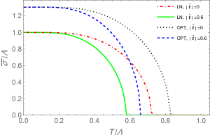
Figure 1: The chiral order parameter, $\bar{\sigma}$, as a function of the temperature at $\mu=0$ and different values of the tilt parameter, $|{\bf\tilde{t}}|$ (in units of $\Lambda$). Both approximations are compared considering the case of $N=2$.

Our prediction for $T_{c}$, given by Eq. (37), reproduces the result from Ref. Kneur:2007vj in the limit ${\tilde{t}}\rightarrow 0$ and the result from Ref. Gomes:2021nem in the limit $N\rightarrow\infty$. The behavior of the critical temperature as a function of the tilting parameter is shown in Fig. 2.

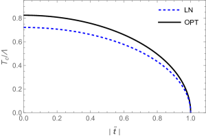
Figure 2: The critical temperature as a function of the tilt parameter, $|{\bf\tilde{t}}|$, at $\mu=0$ and $N=2$. The dashed line represents the LN result while the continuous line represents the OPT prediction.

The results shown in this figure indicate that finite $N$ effects are enhanced at lower values of $|{\bf\tilde{t}}|$ when the difference between the values of $T_{c}$ predicted by both approximations is larger. In particular, the $T_{c}$ value predicted by the OPT is larger than the one predicted by the LN approximation, which is expected since the value of ${\bar{\sigma}}(0)$ predicted by the latter is also larger. As $|{\bf\tilde{t}}|$ increases, this difference decreases such that both approximations predict $T_{c}\to 0$ as $|{\bf\tilde{t}}|\to 1$ in accordance with Eq. (37). Therefore, the presence of a tilt in the Dirac cone inhibits CSB.

V.3 The $T=0$ and $\mu\neq 0$ case

Let us now consider the $T=0$ and $\mu\neq 0$ case. Assuming a positive and nonnull chemical potential, in the limit $T\rightarrow 0$, one finds $n_{p}(\mu_{t})=\Theta(\mu_{t}-\omega_{p})$ and $\bar{n}_{p}(\mu_{t})=\Theta(-\mu_{t}-\omega_{p})=0$ where $\Theta(x)$ represents the Heaviside step function. This result is valid for all $\mu>0$, since $|\tilde{{\bf t}}\cdot{\bf p}|<\omega_{p}$. Therefore, assuming $\eta>0$ and $\mu>0$, one has

$$I_{0}=-\frac{\eta^{3}}{6\pi}+\left(\frac{\eta^{3}}{6\pi}-\frac{\eta^{2}\tilde{\mu}}{4\pi}+\frac{\tilde{\mu}^{3}}{12\pi}\right)~{}\Theta\left(\tilde{\mu}-\eta\right),$$ (38)

where we have defined $\tilde{\mu}={\mu}(1-|\tilde{\bf t}|^{2})^{-1/2}$ while $p_{F}$ denotes the Fermi momentum. The latter can be obtained from the inequality $\mu+|\tilde{\bf t}|p\cos\theta-\sqrt{p^{2}+\eta^{2}}>0$. Namely,

$$p_{F}=\sqrt{\frac{\mu^{2}-\eta^{2}(1-|{\bf\tilde{t}}|^{2}\cos^{2}\theta)}{\left(1-|{\bf\tilde{t}}|^{2}\cos^{2}\theta\right)^{2}}}+\frac{\mu|{\bf\tilde{t}}|\cos\theta}{1-|{\bf\tilde{t}}|^{2}\cos^{2}\theta}\,,$$ (39)

from which the standard Fermi momentum, $p_{F}=\sqrt{\mu^{2}-\eta^{2}}$, is recovered when $|{\bf\tilde{t}}|=0$. Requiring $p_{F}\in\mathbb{R}$ implies that $\mu^{2}-\eta^{2}(1-|{\bf\tilde{t}}|^{2})>0$, which, in turn, produces the step function $\Theta\left(\tilde{\mu}-\eta\right)$. Likewise, for the integral $I_{1}$, one obtains

$$I_{1}=-\frac{\eta}{4\pi}-\frac{1}{4\pi}\left(\tilde{\mu}-\eta\right)\Theta\left(\tilde{\mu}-\eta\right)~{}~{}.$$ (40)

Note that $2\eta I_{1}=\frac{\partial I_{0}}{\partial\eta}$, as expected. Next, the integral $I_{2}$ can be written as

$$I_{2}=\frac{1}{8\pi\sqrt{1-|{\bf\tilde{t}}|^{2}}}\left(\tilde{\mu}^{2}-\eta^{2}\right)\Theta\left(\tilde{\mu}-\eta\right)~{}~{}.$$ (41)

To obtain $I_{3}$, one should first notice that the use of polar coordinates, ${\bf p}=p(\cos\theta,\sin\theta)$, ${\bf q}=q(\cos\theta^{\prime},\sin\theta^{\prime})$, leads to $\tilde{{\bf t}}\cdot{\bf p}=|{\bf\tilde{t}}|p\cos\theta$ and $\tilde{{\bf t}}\cdot{\bf q}=|{\bf\tilde{t}}|q\cos\theta^{\prime}$. One then gets

$$I_{3}=\frac{1}{64\pi^{2}}\frac{|{\bf\tilde{t}}|^{2}}{1-|{\bf\tilde{t}}|^{2}}\left(\tilde{\mu}^{2}-\eta^{2}\right)^{2}\Theta\left(\tilde{\mu}-\eta\right)\,$$ (42)

which explicitly shows that $I_{3}=0$ when $|{\bf\tilde{t}}|=0$. Therefore, the OPT effective potential at first-order can be written as

$$\!\!\!\!\!\frac{V_{\rm eff}(\mu)}{N} = \frac{-1}{\pi\xi_{x}\xi_{y}v_{F}^{2}}\left\{\frac{\delta}{2}\sigma^{2}\Lambda-\frac{\eta^{3}}{3}+\delta{(\eta-\sigma)\eta^{2}}+\frac{\delta\eta^{4}}{8N\Lambda}\right.$$

$$+\; \!\!\!\!\!\!\left[\frac{\eta^{3}}{3}-\frac{\eta^{2}\tilde{\mu}}{2}+\frac{\tilde{\mu}^{3}}{6}+\delta(\eta-\sigma)\eta(\tilde{\mu}-\eta)\right.$$

$$+\; \!\!\!\!\!\!\left.\left.\frac{\delta(\tilde{\mu}^{2}-\eta^{2})\eta^{2}}{8N\Lambda}+\frac{\delta\left(\tilde{\mu}^{2}-\eta^{2}\right)^{2}}{32N\Lambda}\right]\Theta\left(\tilde{\mu}-\eta\right)\right\}.$$

In Fig. 3 we show $V_{\rm eff}$, given by Eq. (LABEL:PotEffMUnulo2), as a function of $\sigma$ and for different values of the tilt parameter. As one can notice, the figure displays a typical first-order transition pattern. Namely, at $\mu=0$ the effective potential has a maximum at $\sigma=0$ and a unique minimum at ${\bar{\sigma}}\neq 0$. As $\mu$ increases, the (unstable) maximum at $\sigma=0$ becomes a point of inflection, marking the emergence of the first spinodal. A slight increase of the chemical potential value converts the inflection point, at $\sigma=0$, into a (metastable) local minimum, while a (stable) global minimum remains fixed at ${\bar{\sigma}}\neq 0$. As expected, the two non-degenerate minima are separated by a barrier. Then, when $\mu=\mu_{c}$, the two minima become degenerate allowing for a first-order phase transition. When $\mu$ is slightly higher than $\mu_{c}$, the minimum at the origin becomes stable (global) while the one sitting at ${\bar{\sigma}}\neq 0$ becomes metastable (local). By further increasing the chemical potential one eventually reaches the second spinodal, where the local minimum at ${\bar{\sigma}}\neq 0$ becomes a point of inflection before disappearing when $\mu$ further increases. Since the order parameter is associated with the value of $\sigma$ at the (global) minimum, the above discussion allows us to forecast that this quantity will suffer a discontinuous transition from ${\bar{\sigma}}=\Lambda/{\mathcal{F}(N)}^{2}\to{\bar{\sigma}}=0$ at the coexistence chemical potential, $\mu=\mu_{c}$.

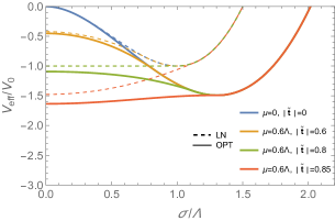
Figure 3: The effective thermodynamic potential at $T=0$ and $N=2$, for different values of $\mu$ and $|{\bf{\tilde{t}}}|$, as predicted by the LN approximation and the OPT (at first order). The normalization $V_{0}$ is given by $V_{0}/N=\Lambda^{3}/(6\pi\xi_{x}\xi_{y}v_{F}^{2})$, as in Ref. Gomes:2021nem .

In principle, to be able to analyze how the chiral parameter behaves with $\mu$ one can proceed as in the previously discussed case $(T\neq 0,\mu=0)$ by considering the gap equation,

$${\bar{\sigma}}=\frac{1}{\Lambda}\left[{\bar{\eta}}^{2}+{\bar{\eta}}({\tilde{\mu}}-{\bar{\eta}})\Theta\left(\tilde{\mu}-\eta\right)\right]\,.$$ (44)

However, now the integrals $I_{2}$ and $I_{3}$ do not vanish and the optimization equation becomes much more involving. As a matter of fact, for certain values of $\mu$ one may get three different $\bar{\eta}$ solutions such that the gap equation will give three different values for $\bar{\sigma}$, which ultimately describe the three extrema associated with the unstable, metastable and stable phases. In practice, one can adopt a more pragmatic approach to obtain ${\bar{\sigma}}(\mu)$ by determining the global minimum of $V_{\rm eff}(\mu)$ in a numerical fashion as we do here. The result is shown in Fig. 4.

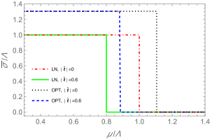
Figure 4: The chiral order parameter, $\bar{\sigma}$ (in units of $\Lambda$), as a function of $\mu/\Lambda$ for different values of the tilt parameter when $N=2$. In each case the values ${\bar{\sigma}}\neq 0$ and ${\bar{\sigma}}=0$ are linked by the (vertical) Maxwell line.

As already mentioned, by evaluating the optimized effective potential at its minimum one obtains the optimized thermodynamic potential, $\Omega=V_{\rm eff}({\bar{\sigma}},{\bar{\eta}})$ which allows us to obtain the net charge density, $n$. In the case of first order transitions $n$ represents an interesting physical observable which can also be viewed as an alternative order parameter. In a thermodynamically consistent evaluation, the net charge number density is written as

$$n=-\frac{\partial\Omega}{\partial\mu}\,.$$ (45)

Now, recalling that ${\bar{\sigma}}$ and ${\bar{\eta}}$ are $\mu$-dependent and upon applying the chain rule one gets

$$\frac{\partial\Omega}{\partial\mu}=-n+\frac{\partial{\bar{\eta}}}{\partial\mu}\frac{\partial\Omega}{\partial{\bar{\eta}}}+\frac{\partial{\bar{\sigma}}}{\partial\mu}\frac{\partial\Omega}{\partial{\bar{\sigma}}}\,,$$ (46)

which is thermodynamically consistent since the optimization criterion and the gap equation respectively require $\partial\Omega/\partial{\bar{\eta}}=0$ and $\partial\Omega/\partial{\bar{\sigma}}=0$. More explicitly, one can write the number density per fermionic specie as

$$\frac{n}{N} = \frac{1}{\pi\xi_{x}\xi_{y}v_{F}^{2}\sqrt{1-|{\bf\tilde{t}}|^{2}}}\left[\frac{1}{2}({\tilde{\mu}}^{2}-{\bar{\eta}}^{2})+\delta{\bar{\eta}}({\bar{\eta}}-{\bar{\sigma}})\right.$$ (47)

$$+ \left.\delta\frac{{\bar{\eta}}^{2}{\tilde{\mu}}}{4N\Lambda}+\delta\frac{{\tilde{\mu}}({\tilde{\mu}}^{2}-{\bar{\eta}}^{2})}{8N\Lambda}\right]\Theta\left(\tilde{\mu}-\eta\right)\,.$$

In Fig. 5 we illustrate the behavior of the charge number density for different values of the tilt parameter as predicted by both approximations considered in this work when $N=2$. Following Ref. Gomes:2021nem we have normalized $n/N$ by $n_{0}/N=\Lambda^{2}/(2\pi\xi_{x}\xi_{y}v_{F}^{2})$ which represents the LN prediction at $t=0$. The figure clearly shows the coexistence of two phases, with $n=0$ (vacuum) and $n\neq 0$ (charged), at the same $\mu_{c}$. In principle, the phase with vanishing charge density can represent an insulator, while the phase with finite charge density can represent a metal. Within this scenario, the coexistence phase could represent a semimetal.

The inspection of Eq. (47) reveals that the tilt, as well as finite $N$ effects, favor higher density values as Fig. 5 confirms.

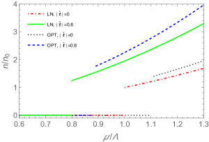
Figure 5: The fermionic number density, normalized by $n_{0}$ (see text), as a function of the chemical potential (in units of $\Lambda$) for $N=2$. Each curve indicates that a given $\mu_{c}$ the “vacuum” ($n=0$), which represents the insulator phase, coexists with matter at a certain finite charge density (metallic phase). This coexistence phase could represent a semimetal.

We can now attempt to find an equation to determine the numerical value of the coexistence chemical potential. Following the reasoning of Ref. Kneur:2007vm , this can be achieved by equating the values of the effective potential at the degenerate minima, $V_{\rm eff}({\bar{\sigma}}\neq 0,\mu_{c}<{\bar{\sigma}})$ and $V_{\rm eff}({\bar{\sigma}}=0,\mu_{c}>{\bar{\sigma}})$. This guarantees that, despite having distinct densities, the two coexisting phases share the same pressure (and temperature), as thermodynamics requires. From section V.1, one can easily obtain the minimum corresponding to the vacuum phase,

$$\frac{V_{\rm eff}({\bar{\sigma}}\neq 0,\mu_{c}<{\bar{\sigma}})}{N}=-\frac{1}{6\pi\xi_{x}\xi_{y}v_{F}^{2}}\left(\frac{\Lambda}{{\mathcal{F}(N)}}\right)^{3},$$ (48)

To obtain $V_{\rm eff}({\bar{\sigma}}=0,\mu_{c}>{\bar{\sigma}})$, one can use the gap equation (44) to set ${\bar{\eta}}={\bar{\sigma}}\equiv 0$ in Eq. (LABEL:PotEffMUnulo2). This yields the minimum related to the charged phase

$$\frac{V_{\rm eff}({\bar{\sigma}}=0,\mu_{c}>{\bar{\sigma}})}{N}=-\frac{\tilde{\mu}_{c}^{3}}{6\pi\xi_{y}\xi_{x}v_{F}^{2}}\left(1+\frac{3\tilde{\mu}_{c}}{16N\Lambda}\right)\,,$$ (49)

with the obvious notation $\tilde{\mu}_{c}=\mu_{c}(1-|\tilde{\bf t}|^{2})^{-1/2}$. Therefore, the coexistence chemical potential satisfies the equation

$$\left(\frac{\Lambda}{{\mathcal{F}(N)}}\right)^{3}-\tilde{\mu}_{c}^{3}\left(1+\frac{3\tilde{\mu}_{c}}{16N\Lambda}\right)=0.$$ (50)

Then, when $N=2$, Eq. (50) sets the OPT prediction to $\mu_{c}\approx 1.106\Lambda(1-|\tilde{\bf t}|^{2})^{-1/2}$ while the LN approximation predicts $\mu_{c}=\Lambda(1-|\tilde{\bf t}|^{2})^{-1/2}$. In Fig. 6, we compare the results for the coexistence chemical potential, obtained with both approximations, as a function of the tilt parameter. The OPT predicts a higher value for $\mu_{c}$ which, once again, could be expected owing to the fact that ${\bar{\sigma}}(0)$ predicted by this approximation is larger. The difference between the OPT and LN predictions decreases as the the tilt increases since $\mu_{c}\to 0$ as $|{\bf\tilde{t}}|\to 1$.

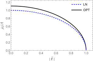
Figure 6: The coexistence chemical potential as a function of the tilt parameter, $|{\bf\tilde{t}}|$, at $T=0$ and $N=2$. The dashed line represents the LN result while the continuous line represents the OPT prediction.

V.4 The $T\neq 0$ and $\mu\neq 0$ case

Finally considering the case of finite temperatures and densities one needs to scrutinize the effective potential (or free energy) in order to locate the regions where first- and second-order phase transitions occur. Then, one should be able to find the tricritical point, located at ($T_{\rm tcr},\mu_{\rm tcr}$), which separates the regions displaying distinct phase transitions. Proceeding in a numerical fashion one obtains the results displayed in Fig. 7. This figure portraits the complete phase diagram for the GN model with tilted Dirac cone on the plane spanned by the control parameters at hand ($T$ and $\mu$). The colored dots associated to the OPT curves, for $|{\bf\tilde{t}}|=0$ and $|{\bf\tilde{t}}|=0.6$, indicate the position of the respective tricritical points. Above these points, the chiral transition is of the second kind. The shaded areas that appear in the OPT results, below the tricritical points, are associated with first-order phase transitions. Such regions are delimited by spinodal lines which indicate the presence of metastable phases. In between the two spinodal lies a first-order transition line over which two stable phases (with distinct densities) coexist at the same $T$ and $\mu$.

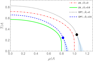
Figure 7: The phase diagram for $N$ = 2 on the $T-\mu$ plane. The OPT tricritical points are indicated by the large dots. The second-order transition is represented by the lines above the tricritical points. The OPT predicts that first-order transitions occur within the shadowed low-$T$ region below the tricritical points. This region is bounded by two spinodal lines while the central line marks the exact location where the transition occurs. The LN approximation predicts a second-order phase transition at all finite temperatures and a first-order phase transition at $T=0$ only.

To further analyze the nature of the phase transitions let us first recall that, contrary to the chemical potential, the number density does not represent a control parameter. Nevertheless, when combined with the temperature this thermodynamical observable offers an interesting alternative in providing deeper insights into the possible transition patterns, especially those related to first-order phase transitions. This alternative framework is represented by the phase diagram on the $T-n$ plane, as Fig. 8 displays. This figure shows that below the tricritical temperature, the OPT predicts a first-order phase transition region which is bounded by binodal lines. One can also see that for a given temperature, lower than $T_{\rm tcr}$, the binodal indicates the existence of two distinct density values at which the different phases (symmetric and nonsymmetric) coexist. The inner region is associated to the existence of a mixed phase, characterized by metastable and unstable states. Recalling that within the present model, the typical gap energy (at $T=\mu=0$) has a value close to $\Lambda$ the OPT therefore predicts the existence of a mixed phase from $T=0$ to roughly $T\sim\Lambda/4$. The possible existence of such a mixed phase, missed by the LN (and mean field) approximation, represents our main result.

For completeness, in Table 1, we show the predictions for the tricritical control parameters, $T_{\rm tcr}$ and $\mu_{\rm trc}$, as well as for the charge density at this location, $n_{\rm trc}=n(T_{\rm tcr},\mu_{\rm tcr})$, considering some representative values of the tilt parameter. The numerical values of $T_{\rm tcr}$ and $\mu_{\rm trc}$ can be obtained in different ways. Here, we have numerically determined the values at which the two degenerate minima, associated with the first order transition, merge and become the unique minimum (at $\bar{\sigma}=0$), characterizing a phase transition of the second kind. A possible alternative to determine $T_{\rm tcr}$ and $\mu_{\rm trc}$ is to apply Landau’s expansion to the free energy ($V_{\rm eff}$), following the prescription described in Ref. Kneur:2007vj (where only the untilted case has been considered).

The results shown in Table 1 indicate that the values of the tricritical control parameters, $T_{\rm tcr}$ and $\mu_{\rm trc}$, decrease as $|{\bf\tilde{t}}|$ increases. This result could be anticipated since the tilt enhances the shrinkage of the region with broken chiral symmetry, as we have already discussed. On the other hand, the observable $n_{\rm tcr}$ assumes higher values as the tilt increases.

Table 1: Values for the tricritical temperature, tricritical chemical potential, and charge density (at the tricritical point) for different values of the tilting parameter, as predicted by both approximations when $N=2$.

Method	$|{\bf\tilde{t}}|$	$T_{\rm tcr}/\Lambda$	$\mu_{\rm trc}/\Lambda$	$n_{\rm tcr}/n_{0}$
	0	0	1.0	1.0
	0.3	0	0.954	1.048
LN	0.6	0	0.800	1.251
	0.9	0	0.436	2.299
	0	0.305	1.040	1.557
	0.3	0.285	0.990	1.613
OPT	0.6	0.245	0.820	1.902
	0.9	0.135	0.455	3.617

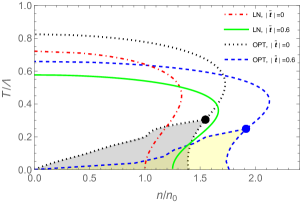
Figure 8: The phase diagram for $N$ = 2 on the $T-n/n_{0}$ plane. The OPT tricritical points are indicated by the large dots. The second-order transition is represented by the lines above the tricritical points. The OPT predicts that first-order transitions occur within the shadowed low-$T$ region below the tricritical points. This region is bounded by binodal lines which, for a given temperature, indicate the two co-existing densities. The LN approximation predicts a second-order phase transition at all finite temperatures and a first-order phase transition at $T=0$ only.

V.5 Applications

It should be noticed that Weyl like materials are still rather rare. The difficulty to find 2DWSM lies in the fact that a two-dimensional fermionic system does not have topological protection against gap formation in comparison to the 3D counterpart. Despite of this, some materials are known, as for instance, quinoid-type graphene and $\alpha$-(BEDT-TTF)${}_{2}I_{3}$ organic conductors goerbig2008 ; Hirata and, more recently, the cases of Epitaxial Bismuthene 2303.02971 and porous Si/Ge structures that have been proposed as a 2DWSM 2305.05756 . Several candidates for bidimensional Dirac materials have also been proposed, such as Si and Ge honeycomb lattices as well as porous and crystalline organic structures among a myriad of other possibilities (for a recent review, see, e.g., Ref. runyu . Keeping that in mind let us discuss some implications of our results, based on some of the available experimental data for some of the existing bi-dimensional materials.

We can now use a phenomenological input in order to fix the GN scale, $\Lambda$, so that our theoretical predictions can be ultimately compared to some of the available experimental results. The aim of such exercise is just to check whether the OPT predictions lie within the ball park range of the available experimental data. As a starting point, we can consider that current experiments are carried out at room temperature ($300\,K$) or close to it. We will also suppose that these temperatures lie within the region of the second-order phase transition and just above the (highest) tricritical temperature (see Fig. 8 for reference).

According to the results shown in Table 1, the highest value for the tricritical temperature is $T_{\rm trc}=0.305\,\Lambda$, which occurs for $|{\bf\tilde{t}}|=0$. We can then assume that the room temperature ($300\,K$) lies slightly above $T_{\rm trc}$, but still in the second-order transition region and take for example $T_{\rm exp}=0.35\,\Lambda=0.0258\,{\rm eV}>T_{\rm trc}$. This then allows us to fix the GN scale to be $\Lambda_{\rm exp}=0.0738\,{\rm eV}$. Note that, since $\Lambda\propto 1/|\lambda|$, this is basically the equivalent of fixing the coupling, which represents the only energy scale present in the $(2+1)-$dimensions GN model. Considering this value of $\Lambda$ as the numerical scale used to produce Fig. 7 one gets, at $T=T_{\rm exp}$, the values $\mu_{\rm exp}\approx 1.02\Lambda_{\rm exp}=0.0753\,{\rm eV}$ and ${\bar{\sigma}}_{\rm exp}\approx 1.3\Lambda_{\rm exp}=0.096\,{\rm eV}$ for the chemical potential and gap energy respectively. As discussed in Ref. graph , both values lie within the bounds of phenomenological predictions. Finally, one can check the actual charge density number at $T_{\rm exp}$ by taking $n/n_{0}\approx 1.6$ (see Fig. 7 and Table 1). Then, using

$$n_{\rm exp}=\frac{N}{2\pi\xi_{x}\xi_{y}v_{F}^{2}}\left(\frac{n}{n_{0}}\right)\Lambda_{\rm exp}^{2},$$ (51)

at $N=2$, $\xi_{x}=\xi_{y}\equiv 1$, and $v_{F}/c=1/300$ one gets $n=1.62\times 10^{10}{\rm cm}^{-2}$ which is very similar to the result $n=1.2\times 10^{10}{\rm cm}^{-2}$ obtained for instance in experiments devoted to measure the Casimir interaction between a Au-coated sphere and a graphene-coated ${\rm SiO}_{2}$ layer on the top of a Si plate graph . To reach the first-order transition region (with its mixed phase) one should further lower the temperature. For example, at $|{\bf\tilde{t}}|=0$ one may set $T=0.3\Lambda=0.0221\,{\rm eV}<T_{\rm trc}$, which corresponds to $255.29\,K$ whereas, at $|{\bf\tilde{t}}|=0.6$, one can consider $T=0.235\Lambda=0.0173\,{\rm eV}<T_{\rm trc}$, which corresponds to $200\,K$.

By going to extremely low temperatures, one eventually will reach a region where two phases, with very different densities, can coexist. For example, when $|{\bf\tilde{t}}|=0$ and $T=0.05\Lambda=\,0.037{\rm eV}$ ($42.82\,K$) one can have the low density ($n=0.2125\times 10^{10}\,{\rm cm}^{-2}$) gapped (nonsymmetric) phase coexisting with the high density ($n=1.405\times 10^{10}\,{\rm cm}^{-2}$) nongapped (symmetric) phase.

Furthermore, recent numerical work on Weyl semimetals crippa have shown a first type topological quantum phase transition as a function of the interaction. It would be interesting to look at this type of model in regimes where a similar transition, as a function of the chemical potential and temperature, can appear, as predicted by our results.

Finally, one should also note that from some of the available experimental results on (quasi-)planar materials (such as for example in Ref. [54]), the linear simple Weyl cone structure is well described for energies below and around ${\cal O}(10{\rm meV})$. At appropriate values of the energy scale ($\Lambda$), and for corresponding temperature and chemical potential not much higher than $\Lambda$, the possible nonlinearities in the dispersion relation are expected to remain small and our results should provide a reasonable qualitative description of the real physical systems. In particular, the estimates provided above, fall in the ballpark of what one would expect for the linear (relativistic) dispersion to be a reasonable approximation.

VI Conclusions

Considering the tilted $(2+1)$-dimensional GN model, we have analyzed the phase transition patterns associated with the breaking or restoration of chiral symmetry within planar Weyl type of materials. In order to incorporate finite-$N$ effects, we have employed the OPT approximation to evaluate the effective thermodynamic potential (Landau’s free energy) to the first non-trivial order. This strategy has allowed us to consider a two-loop contribution (of order $1/N$) to improve over existing large-$N$ results Gomes:2021nem .

Starting with the simplest ($T=\mu=0$) case, where the tilt does not contribute, we have reproduced previous OPT results confirming that finite $N$ effects produce chiral order parameter values that are higher than the ones predicted at large-$N$. Proceeding to the case of thermal matter at vanishing densities, we have shown that the system undergoes a second-order phase transition at a critical temperature given by $T_{c}=\Lambda(1-|{\bf\tilde{t}}|^{2})^{1/2}\,[2\ln 2\mathcal{F}(N)]^{-1}$. This result suggests that finite $N$ corrections lead to phase transitions taking place at higher $T_{c}$ values than those predicted by the LN approximation. On the other hand, the tilt (parametrized by $|{\bf\tilde{t}}|$) favors a more disordered phase such that $T_{c}\to 0$ as $|{\bf\tilde{t}}|\to 1$. Considering the case of a finite chemical potential at zero temperature, we have once again reproduced previous predictions confirming that chiral symmetry is restored through a first-order phase transition. The coexistence chemical potential, $\mu_{c}$, at which the transition takes place, increases with decreasing values of $N$. Also, in this case, we observe that the tilt enhances the restoration of chiral symmetry since $\mu_{c}\to 0$ as $|{\bf\tilde{t}}|\to 1$. In summary, the phase transition patterns predicted by the LN and by the OPT for these three particular cases are qualitatively the same. From a more quantitative perspective, the OPT predictions indicate that finite $N$ effects favor the ordered phase.

Our investigation shows that the alluded qualitative agreement ceases to be observed at finite temperature and chemical potential, when the phase transition boundaries predicted by both approximations become very different. As it is well established, the LN phase diagram displays a second-order transition line for all $T>0$, since a first-order transition is predicted to occur only at $T=0$. However, we have explicitly shown that this situation turns out to be an artifact of the LN approximation, and already at the first non-trivial order, the OPT is capable of predicting a phase diagram which is more in line with what continuity arguments Kogut:1999um suggest. More specifically, finite $N$ effects produce a first-order transition line that starts at $T=0$ and terminates at a tricritical point roughly located at a (tricritical) temperature whose value is about $20\%$ to $30\%$ of the value of the “in vacuum” gap energy ($\sim\Lambda$). Physically, one of the most important consequences of the first-order transition line predicted here is that it allows for two distinct phases of a Weyl type of material to co-exist at low temperatures. Therefore, a Weyl-type of planar materials should have a phase transition structure much richer than one predicted by the LN (or mean-field) approximation. Here, the prediction of such a mixed phase has been entirely derived upon using quantum field theory methods. Possible further extensions of the present application might be for example to extend the LN study of superconducting phase transitions in planar fermionic models with Dirac cone tilting Gomes:2022dmf such as to include finite $N$ effects and also looking for the effects of magnetic fields when applied to the system.

- (1) K. S. Novoselov, A. K. Geim, S. V. Morozov, D. Jiang, M. I. Katsnelson, I. V. Grigorieva, S. V. Dubonos and A. A. Firsov, Two-dimensional gas of massless Dirac fermions in graphene, Nature 438, 197 (2005).
- (2) A. G. Grushin, Consequences of a condensed matter realization of Lorentz violating QED in Weyl semi-metals, Phys. Rev. D 86, 045001 (2012).
- (3) S. Tchoumakov, M. Civelli, and M. O. Goerbig, Magnetic-field-induced relativistic properties in type-I and type-II Weyl semimetals, Phys. Rev. Lett. 117, 086402 (2016).
- (4) A. A. Soluyanov, D. Gresch, Z. Wang, Q. Wu, M. Troyer, X. Dai and B. A. Bernevig, Type-II Weyl semimetals, Nature 527, 495 (2015).
- (5) X. Wan, A. Turner, A. Vishwanath and S. Y. Savrasov, Topological semimetal and Fermi-arc surface states in the electronic structure of pyrochlore iridates, Phys. Rev. B 83, 205101 (2011).
- (6) M. O. Goerbig, J.-N. Fuchs, G. Montambaux, and F. Piéchon, Tilted anisotropic Dirac cones in quinoid-type graphene and , Phys. Rev. B 78, 045415 (2008).
- (7) M. Z. Hasan and J. E. Moore, Three-Dimensional Topological Insulators, Ann. Rev. Condensed Matter Phys. 2, 55 (2011).
- (8) V. A. Kostelecký, R. Lehnert, N. McGinnis, M. Schreck and B. Seradjeh, Lorentz violation in Dirac and Weyl semimetals, Phys. Rev. Res. 4, 023106 (2022).
- (9) D. J. Gross and A. Neveu, Dynamical symmetry breaking in asymptotically free field theories, Phys. Rev. D 10, 3235 (1974).
- (10) H. Caldas, J. L. Kneur, M. B. Pinto and R. O. Ramos, Critical dopant concentration in polyacetylene and phase diagram from a continuous four-Fermi model, Phys. Rev. B 77, 205109 (2008).
- (11) H. Caldas and R. O. Ramos, Magnetization of planar four-fermion systems, Phys. Rev. B 80, 115428 (2009).
- (12) R. O. Ramos and P. H. A. Manso, Chiral phase transition in a planar four-Fermi model in a tilted magnetic field, Phys. Rev. D 87, 125014 (2013).
- (13) V. C. Zhukovsky, K. G. Klimenko and T. G. Khunjua, Superconductivity in chiral-asymmetric matter within the (2 + 1)-dimensional four-fermion model, Moscow Univ. Phys. Bull. 72, 250 (2017).
- (14) D. Ebert, K. G. Klimenko, P. B. Kolmakov and V. C. Zhukovsky, Phase transitions in hexagonal, graphene-like lattice sheets and nanotubes under the influence of external conditions, Ann. Phys. 371, 254 (2016).
- (15) K. G. Klimenko and R. N. Zhokhov, Magnetic catalysis effect in the (2+1)-dimensional Gross-Neveu model with Zeeman interaction, Phys. Rev. D 88, 105015 (2013).
- (16) K. G. Klimenko, R. N. Zhokhov and V. C. Zhukovsky, Superconductivity phenomenon induced by external in-plane magnetic field in (2+1)-dimensional Gross-Neveu type model, Mod. Phys. Lett. A 28, 1350096 (2013).
- (17) T. G. Khunjua, K. G. Klimenko and R. N. Zhokhov, Spontaneous non-Hermiticity in the (2+1)-dimensional Gross-Neveu model, Phys. Rev. D 105, 025014 (2022).
- (18) Y. M. P. Gomes and R. O. Ramos, Tilted Dirac cone effects and chiral symmetry breaking in a planar four-fermion model, Phys. Rev. B 104, 245111 (2021).
- (19) Y. M. P. Gomes and R. O. Ramos, Superconducting phase transition in planar fermionic models with Dirac cone tilting, Phys. Rev. B 107, 125120 (2023).
- (20) K. G. Klimenko, Phase structure of generalized Gross-Neveu models, Z. Phys. C 37, 457 (1988).
- (21) B. Rosenstein, B. J. Warr and S. H. Park, Thermodynamics of (2+1)-dimensional four Fermi models, Phys. Rev. D 39, 3088 (1989).
- (22) B. Rosenstein, B. J. Warr and S. H. Park, The four Fermi theory is renormalizable in (2+1)-dimensions, Phys. Rev. Lett. 62, 1433 (1989).
- (23) J. B. Kogut and C. G. Strouthos, Chiral symmetry restoration in the three-dimensional four-fermion model at nonzero temperature and density, Phys. Rev. D 63, 054502 (2001).
- (24) S. Hands, A. Kocic and J. B. Kogut, Four-Fermi theories in fewer than four dimensions, Ann. Phys. 224, 29 (1993).
- (25) S. Hands, A. Kocic and J. B. Kogut, The four Fermi model in three dimensions at nonzero density and temperature, Nucl. Phys. B 390, 355 (1993).
- (26) A. Okopińska, Nonstandard expansion techniques for the effective potential in quantum field theory, Phys. Rev. D 35, 1835 (1987).
- (27) A. Duncan and M. Moshe, Nonperturbative physics from interpolating actions, Phys. Lett. B 215, 352 (1988).
- (28) J. L. Kneur, M. B. Pinto, R. O. Ramos and E. Staudt, Updating the phase diagram of the Gross-Neveu model in 2+1 dimensions, Phys. Lett. B 657, 136 (2007).
- (29) J. L. Kneur, M. B. Pinto, R. O. Ramos and E. Staudt, Emergence of tricritical point and liquid-gas phase in the massless 2+1 dimensional Gross-Neveu model, Phys. Rev. D 76, 045020 (2007).
- (30) J. L. Kneur, M. B. Pinto and R. O. Ramos, Phase diagram of the magnetized planar Gross-Neveu model beyond the large-N approximation, Phys. Rev. D 88, 045005 (2013).
- (31) J. J. Lenz, M. Mandl and A. Wipf, Magnetic catalysis in the (2+1)-dimensional Gross-Neveu model, [arXiv:2302.05279 [hep-lat]].
- (32) J. J. Lenz, M. Mandl and A. Wipf, The magnetized (2+1)-dimensional Gross-Neveu model at finite density, [arXiv:2304.14812 [hep-lat]].
- (33) H. B. Nielsen and M. Ninomiya, Absence of Neutrinos on a Lattice. 1. Proof by Homotopy Theory, Nucl. Phys. B 185, 20 (1981) [erratum: Nucl. Phys. B 195, 541 (1982)].
- (34) H. B. Nielsen and M. Ninomiya, Absence of Neutrinos on a Lattice. 2. Intuitive Topological Proof, Nucl. Phys. B 193, 173-194 (1981).
- (35) K. Sasaki and R. Saito, Pseudospin and deformation-induced gauge field in graphene, Prog. Theor. Phys. Suppl. 176, 253 (2008).
- (36) P. L. Zhao, A. M. Wang and G. Z. Liu, Condition for the emergence of a bulk Fermi arc in disordered Dirac-fermion systems, Phys. Rev. B 98, no.8, 085150 (2018).
- (37) J. Wang, Role of four-fermion interaction and impurity in the states of two-dimensional semi-Dirac materials, J. Phys. Condens. Matter 30, no.12, 125401 (2018).
- (38) J. E. Drut and T. A. Lahde, Lattice field theory simulations of graphene, Phys. Rev. B 79, 165425 (2009).
- (39) I. F. Herbut, Interactions and phase transitions on graphene’s honeycomb lattice, Phys. Rev. Lett. 97, 146401 (2006).
- (40) D. T. Son, Quantum critical point in graphene approached in the limit of infinitely strong Coulomb interaction, Phys. Rev. B 75, no.23, 235423 (2007).
- (41) D. E. Sheehy and J. Schmalian, Quantum critical scaling in graphene, Phys. Rev. Lett. 99, 226803 (2007).
- (42) J. E. Drut and T. A. Lahde, Is graphene in vacuum an insulator?, Phys. Rev. Lett. 102, 026802 (2009).
- (43) V. Juricic, I. F. Herbut and G. W. Semenoff, Coulomb interaction at the metal-insulator critical point in graphene, Phys. Rev. B 80, 081405(R) (2009).
- (44) J. Alicea and M. P. A. Fisher, Graphene integer quantum Hall effect in the ferromagnetic and paramagnetic regimes, Phys. Rev. B 74, 075422 (2006).
- (45) I. F. Herbut, Theory of integer quantum Hall effect in graphene, Phys. Rev. B 75, 165411 (2007).
- (46) I. F. Herbut, SO(3) symmetry between Neel and ferromagnetic order parameters for graphene in a magnetic field, Phys. Rev. B 76, 085432 (2007).
- (47) I. L. Aleiner, D. E. Kharzeev and A. M. Tsvelik, Spontaneous symmetry breakings in graphene subjected to in-plane magnetic field, Phys. Rev. B 76, 195415 (2007).
- (48) V. I. Yukalov, Interplay between Approximation Theory and Renormalization Group, Phys. Part. Nucl. 50, 141 (2019).
- (49) P. M. Stevenson, Optimized perturbation theory, Phys. Rev. D 23, 2916 (1981).
- (50) L. H. Ryder, Quantum field theory (Cambridge University Press, Cambridge, 1996).
- (51) M. Le Bellac, Quantum and statistical field theory (Oxford University Press, Oxford, 1992).
- (52) K. G. Klimenko, Three-dimensional Gross-Neveu model at nonzero temperature and in an external magnetic field, Z. Phys. C 54, 323-330 (1992).
- (53) K. G. Klimenko, Gross-Neveu model and optimized expansion method, Z. Phys. C 50, 477-481 (1991).
- (54) M. Hirata, A. Kobayashi, C. Berthier, and K. Kanoda, Interacting chiral electrons at the 2D Dirac points: a review, Rep. Prog. Phys. 84, 036502 (2021).
- (55) Q. Lu, P. V. S. Reddy, H. Jeon, A. R. Mazza, M. Brahlek, W. Wu, S. A. Yang, J. Cook, C. Conner, X. Zhang, et al., Observation of 2D Weyl Fermion States in Epitaxial Bismuthene, arXiv:2303.02971.
- (56) E. V. C. Lopes, R. J. Baierle, R. H. Miwa, T. M. Schmidt, Noncentrosymmetric two-dimensional Weyl semimetals in porous Si/Ge structures, arXiv:2305.05756.
- (57) R. Fan, L. Sun, X. Shao, Y. Li, M. Zhao, Two-dimensional Dirac materials: Tight-binding lattice models and material candidates. Chem Phys Matter, v. 2, 30 (2023).
- (58) G. L. Klimchitskaya, V. M. Mostepanenko, and V. M. Petrov, Conductivity of graphene in the framework of Dirac model: Interplay between nonzero mass gap and chemical potential, Phys. Rev. B 96, 235432 (2017).
- (59) L. Crippa, A. Amaricci, N. Wagner, G. Sangiovanni, J. C. Budich, and M. Capone, Nonlocal annihilation of Weyl fermions in correlated systems, Phys. Rev. Research 2, 012023 (2020).