Kites and Quails: Monetary Policy and Communication with Strategic Financial Markets

Abstract

We develop a simple game-theoretic model to determine the consequences of explicitly including financial market stability in the central bank objective function, when policymakers and the financial market are strategic players, and market stability is negatively affected by policy surprises. We find that inclusion of financial sector stability among the policy objectives can induce an inefficiency, whereby market anticipation of policymakers’ goals biases investment choices. When the central bank has private information about its policy intentions, the equilibrium communication is vague, because fully informative communication is not credible. The appointment of a “kitish” central banker, who puts little weight on market stability, reduces these inefficiencies. If interactions are repeated, communication transparency and overall efficiency can be improved if the central bank punishes any abuse of market power by withholding forward guidance. At the same time, repeated interaction also opens the doors to collusion between large investors, with uncertain welfare consequences.

1 Introduction

We might find ourselves having to act to stabilize the financial markets in order to stabilize the economy. None of us welcomes the charge that monetary policy contains a “Fed put,” but, in extremis, there may be a need for such a put, if not in the strict sense of the finance term, then at least in regard to the direction of policy. How should we communicate about such actions, or, as used to be said of the lender of last resort, should we leave such actions shrouded in constructive ambiguity? 

The Global Financial Crisis of 2007-8 challenged the consensus that monetary policy should focus primarily on inflation (Smets,, 2014). Since then, there has been a significantly revived interest in whether monetary policy should account for financial stability concerns. Indeed, Woodford, (2012) shows that loose monetary policy can increase financial instability and therefore central banks should include such concerns in their objective function.

In addition to such normative questions about central banks’ objective functions, there are two sets of positive questions. First, do we see evidence from the revealed behavior of central banks that they might already have financial stability as part of their objective function? Second, what are the implications of this type of objective function? There is substantial evidence that central banks account for the behavior of financial markets when making decisions. We see this anecdotally from transcripts of policymakers’ meetings, speeches, and other forms of communication. However, there is also more rigorous evidence of this. For example, Shapiro and Wilson, (2022) find that “the FOMC’s loss depends strongly on output growth and stock market performance and less so on their perception of current economic slack.” Moreover, there is evidence that unexpected increases in interest rates lead to a significant decline in bank stock prices as well as a decline in short-term bank profits (e.g. Aharony et al.,, 1986; Flannery and James,, 1984; Busch and Memmel,, 2015; Alessandri and Nelson,, 2015; English et al.,, 2018; Zimmermann,, 2019; Ampudia and van den Heuvel,, 2019; Altavilla et al.,, 2019; Uppal,, 2023; Jiang et al.,, 2023).

Theoretically, there appear to be at least two common approaches in formalizing ways in which central banks care about financial stability. The first relates to policy surprise. For example, Stein and Sunderam, (2018) argue that when central banks surprise the market, it can lead to costly volatility and subsequently instability for highly leveraged financial institutions. The second relates to a directional preference of the financial market participants whereby market participants might prefer low interest rates to high interest rates. This is often related to the ‘Fed Put’ (a term that describes a scenario in which the Federal Reserve keeps interest rates low in order to protect the stock market). Cieslak and Vissing-Jorgensen, (2021) highlight that the Fed Put could result in moral hazard issues.

In our paper, we seek to understand the implications of these modified central bank objective functions when financial institutions are strategic players (i.e., they know the central bank cares about their stability). Using this game-theoretic set-up, we produce a number of contributions to the literature. First, we show that if investors (i.e., financial market participants) face costly readjustments when their investment position is not consistent with the central bank interest rate choice and the central bank internalizes part of this adjustment cost, then the central bank underreacts to shocks to the economy. In a sense, this is consistent with the gradualism approach highlighted by Stein and Sunderam, (2018). It is also similar to a result derived by Caballero and Simsek, (2022). They show that even when the Fed does not agree with the market, because market expectations affect current asset valuations, it can induce the Fed to set an interest rate that partly reflects the market’s view.

Next, we focus specifically on systemic financial institutions as most central banks have explicit mandates to ensure the stability of these institutions. Such institutions are often considered “too big to fail” and so arguably warrant additional supervision by regulators. We derive a solution to the game where these systemic institutions have payoffs that relate to policy surprise and directional preference and central banks are concerned about market readjustment costs. In this set-up, we show that when these institutions have market power, there is a policy distortion. Indeed, the designation of the institutions as being systemic relies on them having some measure of market power. Moreover, there is considerable empirical evidence documenting the growing market power of US banks (see, for instance Corbae and D’Erasmo,, 2021; Corbae and Levine,, 2022) and increasing evidence on the role of bank market power in the transmission of monetary policy (Drechsler et al.,, 2017). Our market power-related distortion is akin to the moral hazard conjecture of Cieslak and Vissing-Jorgensen, (2021). Put simply, given that the central bank is concerned with the stability of these institutions, they are able to take more risk ex-ante knowing the central bank will be accommodative.

We then explore two sets of policies to improve welfare. The first relates to classic papers on the appropriate degree of discretion for central banks. For example, Barro and Gordon, (1983) shows that rules for central bank behavior can be welfare improving, but that given monetary policy is a repeated game between the policymaker and the private agents, it is possible that reputational forces might substitute for formal rules. Our findings relate more closely to the seminal paper by Rogoff, (1985) which finds that social welfare can be improved if the appointed central banker is more hawkish than society (i.e., a central banker who differs from the social objective function as they place a larger weight on inflation-rate stabilization relative to employment stabilization). Akin to the hawk-dove result of Rogoff, (1985), we derive a similar kite-quail result. Specifically, we can show that when the central bank can be of two types: quail (place greater weight on financial institution stability) and kite (place a greater weight on the real sector, i.e., the conventional central bank objective), it is socially optimal to have a central bank that is more kitish than the society.

Finally, we contribute to the growing literature on central bank communication. While there is already a large literature on central bank communication through policy announcements, the focus is largely on communicating a decision (Blinder et al.,, 2008). Indeed, papers as early as Stein, (1989) have explored the problems faced by the Fed in announcing its private information about future policies. Stein, (1989) showed that the Fed can communicate some information about its goals through the cheap talk mechanism of Crawford and Sobel, (1982). However, there is much less research on the effects of central bank communication prior to a decision being made. This is an especially important area given the prevalence of central bank speeches, press releases, and other announcements which are used to “guide” market expectations prior to the decision-making meeting as such communications can themselves influence the policy decision. While there is growing empirical evidence on both formal and informal communication (see, for instance Cieslak et al.,, 2019; Hansen et al.,, 2019; Bradley et al.,, 2020; Morse and Vissing-Jørgensen,, 2020), as far as we are aware, only Vissing-Jorgensen, (2020) explores the issue of this type of communication formally in a theoretical model. However, she does not allow for communication to have any benefit nor does she allow for the market to behave strategically, both features that seem prima facie important in describing communication between central banks and markets. We find that when communication is cheap talk, the optimal central banker is more kitish than when the central bank can commit to full transparency. Interestingly, not only does the central bank better achieves its’ stability goals when a kitish central banker is appointed, but investors benefit due to more transparent communication and market stability.

2 Setting

We model the interaction between the central bank (CB) and a set of market players $I$ using the following stylized three-period setting. At time $t=0$, $CB$ privately observes a shock $\omega_{1}\sim U(-\phi_{1},\phi_{1})$ to the economy-stabilizing policy (i.e., the interest rate consistent with stabilizing the economy), and sends a public message $m\in M=[-\phi_{1},\phi_{1}]$ potentially informative about $\omega_{1}$. At $t=1$, after having observed $\omega_{1}$, each market player $i\in I$ simultaneously chooses an investment position $x_{i}\in X$, based on their expectation of the central bank interest rate, which is observed by the $CB$. Finally, at $t=2$, $CB$ observes a second shock to the economy stabilizing policy, $\omega_{2}\sim U(-\phi_{2},\phi_{2})$, independent from $\omega_{1}$, and finally chooses the policy rate $r\in\mathbb{R}$. The economy-stabilizing policy at the time of the decision is $\omega\in[-\phi,\phi]$, where $\omega=\omega_{1}+\omega_{2}$ and $\phi=\phi_{1}+\phi_{2}$. After the policy decision is made, the game ends and payoffs are realized.

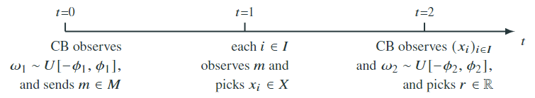
Figure 1: Timeline

Figure 1 provides a graphical representation of the timing. The interpretation of the timeline is as follows. The policy decisions of the Fed are made during meetings of the Fed Open Market Committee (FOMC), occurring once every six weeks, a period of time known as the “FOMC cycle.” We can think of our simple game as occurring within the FOMC cycle. In particular, $t=2$ is the end of the cycle, when the policy decision is made and announced. Within the cycle, official communication occurs at fixed dates, and is meant to increase the transparency of the decision process of the FOMC, as well as provide future guidance to markets (see, e.g., Faust,, 2016, for an extensive discussion of the role of communication). With a simplifying assumption, we assume that that policy-relevant communication occurs only once within the cycle, at $t=0$, where at the time of communication, the policymaker has some uncertainty about the economy-stabilizing policy (captured by $\omega_{2}$). This simplification is consistent with the fact that the speeches of the FOMC chair and vice-chair occur once per cycle, and that the committee observes a mandatory “blackout period” before the occurrence of the end-of-cycle meeting. Finally, in our timeline, investors make the relevant changes to their investment positions before the policy decision $r$ is made. This modelling choice captures the idea that before the decision is made public, at $t=1$ market players choose their investment positions based on their future policy expectations. It allows for “forward guidance” and highlights the economic value that investors derive from correctly predicting future monetary policies.

2.1 Market Surprises and Underreaction

We make two main assumptions that shape the strategic incentives of investors and policymakers in our setting. First, the payoffs of the investors are lower when the mismatch between their investment positions and the policy decision $r$ is greater. Second, the central bank internalizes at least part of this market adjustment cost.

Assumption 1 (Costly Market Readjustments)

Let $X$ = $\mathbb{R}$ and $x_{i}$ denote the element of $X$ chosen by $i$. For $a,b\in\mathbb{R}$, let $S(a,b)=(a-b)^{2}$. We assume that

1. the payoff function of investor $i\in I$ takes the form

   $$u_{i}(x_{i},r)=f^{i}(S(x_{i},r),r)$$

   for $f^{i}:\mathbb{R}^{2}\to\mathbb{R}$ with $f^{i}_{1}<0$, where $f^{i}_{1}$ is the derivative of $f^{i}$ with respect to its first argument;

2. the loss function of the central bank takes the following form. For $\alpha\in(0,1)$,

   $$L_{CB}(x,r,\omega)=\frac{1}{2}(1-\alpha)S(r,\omega)+\frac{1}{2}\alpha g(\bar{S}(x,r)),$$

   for $g:X^{I}\times\mathbb{R}\to\mathbb{R}$ with $g^{\prime}>0$, $g^{\prime\prime}\geq 0$ and $\bar{S}(x,r)$ a weighted average over $\{S(x_{i},r)\}_{i\in I}$.

The assumption has an intuitive interpretation. First, (i) means that the payoff of investor $i$ is, ceteris paribus, decreasing in the mismatch $S(x_{i},r)$ between her investment position $x_{i}$ and the policy $r$. For instance, $x_{i}$ might represent a choice from a continuum of portfolios of financial securities, where portfolio $x_{i}$ is the one performing best at $t=2$ if the policy is $r=x_{i}$. Hence, an investor who chooses a portfolio of securities which performs well given the new policy ($x_{i}$ close to $r$, and $S$ low) at $t=1$ will earn a higher payoff than one who invested poorly ($S$ high). Since at $t=1$ $S$ is minimized in expectation when $i$ holds a position $x_{i}$ which is equal the expected future rate, $S$ is akin to a policy surprise.

Second, assumption (ii), when paired with $\alpha>0$, means that the central bank internalizes the cost of the overall market readjustment due to a policy surprise. The interpretation is analogous to Stein and Sunderam, (2018): unexpected policies can create large fluctuations in asset prices, undermining the financial health of highly leveraged institution. As in Stein and Sunderam, (2018) and Vissing-Jorgensen, (2020), we interpret our loss function $L_{CB}$ as the welfare loss associated to monetary policy, so that $\alpha>0$ means that market instability due to surprises has a negative welfare effect over and beyond the traditional channels of monetary policy.

Not surprisingly, our first simple result is that when the central bank cares about market surprises, it underreacts to shocks in the economy-stabilizing policy that occur after communication. By doing so, policymakers reduce market surprises and the associated welfare cost. This simple intuition is captured by proposition 1, which follows immediately from the game structure and assumption 1.ii.

Proposition 1 (Underreaction)

Let $\sigma$ be any strategy profile played in a PBE of the game, and let $r^{\star}(\sigma,\omega_{1},\omega_{2})$ be the corresponding on-path policy rate chosen by $CB$, expressed as a function of the shocks realizations $(\omega_{1},\omega_{2})$. On the equilibrium path, the central bank under-reacts to the shock $\omega_{2}$, that is $0<\frac{\partial r^{\star}(\sigma,\omega_{1},\omega_{2})}{\partial\omega_{2}}<1$.

In the remainder of the paper, the focus of our analysis will be on a specific payoff specification that satisfies the requirements of assumption 1 and, we believe, delivers interesting insights and policy implications.

3 Interaction with Systemically Important Institutions

We start by analyzing the case where the central bank cares about the financial stability of a set $I$ of systemically important institutions. These investors have a structural interest rate exposure related to their business model that makes their profits depend on the direction of the policy change $r$. In particular, we specify the following forms for the players’ payoffs. For each $i\in I$ and $x_{i},r\in\mathbb{R}$,

$$u_{i}(x_{i},r)=\underbrace{-\frac{1}{2}(x_{i}-r)^{2}}_{\text{policy surprise}}\underbrace{-\beta r}_{\begin{subarray}{c}\text{directional}\\ \text{preference}\end{subarray}}$$ (1)

where $\beta>0$, implying that rate cuts positively impact investors’ payoffs. We interpret $\beta>0$ as investors having a structural positive interest rate exposure deriving from their primary business, meaning that their profits are typically negatively impacted by rate hikes. This is consistent with the findings of Begenau et al., (2020), who show that the traditional business of the US banking sector has typically been characterized by a positive interest rate exposure over the last two decades and Di Tella and Kurlat, (2021) who show, under certain conditions, it is optimal for banks to take losses when interest rates rise. The loss function of the central bank depends on its ability to stabilize the economy and market instability due to a policy surprise. Specifically, for $\omega\in[-\phi,\phi]$, $x\in\mathbb{R}^{I}$ and $r\in\mathbb{R}$,

$$L_{CB}(x,r,\omega)=\underbrace{\frac{1}{2}(1-\alpha)(r-\omega)^{2}}_{\text{conventional loss}}+\underbrace{\alpha\frac{1}{2N}\sum_{i\in I}(r-x_{i})^{2}}_{\text{market readjustment}}.$$ (2)

where $N=|I|$. The loss function is comprised of two terms. The first term is akin to what appears in the standard objective function of New Keynesian models (e.g., Galí,, 2015). Hence, if the welfare weight of systemic investors’ stability was $\alpha=0$, the policy $r=\omega$ would achieve the optimal balance of inflation and economic slack. Note that this standard term already includes the change in banks’ profits due to their traditional-business exposure $\beta$, which could be considered as part of the bank lending channel of monetary policy. The second term in the central bank loss function captures the welfare cost of a financial market readjustment due to policies that surprise large investors. For simplicity, we assume that each systemically relevant institution carries equal weight in contributing to this instability (e.g., they have equal market power), so that the relevant welfare inefficiency is a simple average of the readjustment costs of the investors in $I$.

The solution concept that we adopt for the equilibrium analysis of this simple game is Perfect Bayesian Equilibrium (PBE). We restrict our attention to equilibria in which the central bank choice $r$ at $t=2$ is not contingent on the announcement $m\in M$ at $t=0$. Considering equilibria in which the central bank conditions the policy choice $r$ on previous communication would not yield additional insights, in the absence of reputational considerations. Hence, a strategy for the central bank consists of a communication rule $\sigma_{m}:[-\phi_{1},\phi_{1}]\to\Delta(M)$, mapping realizations of $\omega_{1}$ to a distribution over messages in $M$, and a policy rule $\sigma_{r}:X\times[-\phi_{1},\phi_{1}]\times[-\phi_{2},\phi_{2}]\to\Delta(\mathbb{R})$, mapping investors’ positions and realizations of $(\omega_{1},\omega_{2})$ to distributions over policy decisions. A strategy for market player $i$ is an investment plan $\sigma_{x_{i}}:M\to\Delta(\mathbb{R})$, mapping the central bank’s messages to investment positions. We write $\sigma_{x}=(\sigma_{x_{i}})_{i\in I}$ and denote a generic strategy profile $(\sigma_{m},\sigma_{x},\sigma_{r})$ by $\sigma\in\Sigma$.

Before moving to a general solution for this game, it is useful to identify the communication strategies, investment rule and policy rule that would maximize expected welfare, as this will provide a useful benchmark for equilibrium welfare analyses.

3.1 First Best: The Competitive Benchmark

How would socially optimal communication, investment and policy look like? Given our assumption that $L_{CB}$ is equivalent to the relevant measure of welfare loss in the society, it suffices to ask how the central bank would communicate, invest and set monetary policy if, similarly to a social planner, she could directly choose the investment rule $\sigma_{x}$. The main result of this section is that the ex-ante optimal strategy profile is a PBE of the game where investors chose their strategies autonomously, provided that the banking sector is perfectly competitive. Before stating this result formally and discussing it, it is useful to introduce two additional pieces of notation. First, for some $k\in\mathbb{R}$ and for each $\sigma\in\Sigma$, let $W(\sigma)=k-\mathbb{E}[L_{CB}|\sigma]$ denote the ex-ante welfare when the strategy profile is $\sigma$. For simplicity we assume $k=0$. Second, we let $\hat{W}$ denote the highest achievable welfare in the game if the central bank (or a social planner) could select any strategy profile from $\Sigma$, that is

$$\hat{W}=\max\limits_{\sigma\in\Sigma}W(\sigma)$$ (3)

and let $\hat{\Sigma}$ be the argmax of (3).

The following proposition describes how such “first” best strategy profiles look like, and it identifies the case where a profile in $\hat{\Sigma}$ arises in a market equilibrium.

Proposition 2 (Competitive Benchmark)

$\hat{\Sigma}$ is the set of all strategy profiles presenting each of the following three properties:

1. Communication is fully informative, namely $\sigma_{m}$ partitions $[-\phi_{1},\phi_{1}]$ in singletons: different messages are sent in different states.

2. Investment is unbiased, namely $\sigma_{x_{i}}(m)=\mathbb{E}[\omega_{1}|m,\sigma_{m}]$ for each $i\in I$ and each $m\in M$ played with positive probability in equilibrium;

3. The central bank balances its objectives on the path of play. For $\bar{x}\equiv\frac{1}{N}\sum_{i\in I}x_{i}$, and every $(\omega_{1},\omega_{2})\in[-\phi_{1},\phi_{1}]\times[-\phi_{2},\phi_{2}]$,

   $$\sigma_{r}(\omega_{1},\omega_{2},x)=(1-\alpha)\omega+\alpha\bar{x},$$

   holds if $x_{i}=\omega_{1}$ for all $i\in I$.

Additionally, there exist an equilibrium profile $\sigma^{com}$ such that $(i),(ii)$ and $(iii)$ hold at the limit for $N\to\infty$.

The proof is in the appendix. The three properties of proposition 2 have intuitive interpretations: the central bank communicates all available information $\omega_{1}$ about its’ expected future policy, investment positions minimize expected readjustments given the expectations about the economy-stabilizing rate $\omega$ which are formed after communication, and the final policy is chosen to optimally balance stabilization of the economy and of financial markets. Perhaps more subtly, (i), (ii) and (iii) taken together imply that in this type of game, $\hat{W}$ does not depend on $N$, so that looking at the mismatch between $\hat{W}$ and the ex-ante expected welfare achievable in equilibrium for different level of competitiveness $N$ is meaningful.

The main implication of the proposition is that when there is perfect competition between systemic investors (i.e., $N\to\infty$), there is an equilibrium $\sigma^{com}$ that achieves the maximum welfare $\hat{W}$ that could be obtained by a benevolent planner. The intuition is as follows. First, it is easily verified that in every PBE strategy profile (including $\sigma^{com}$), the central bank uses the same policy rule $\sigma^{\star}_{r}$, that selects a rate lying between $\omega$ and $\bar{x}$, optimally balancing the two stability objectives. In particular, $\sigma^{com}_{r}(\omega_{1},\omega_{2},x)=\sigma^{\star}_{r}(\omega_{1},\omega_{2},x)=(1-\alpha)\omega+\alpha\bar{x}$, which satisfies property (iii) of proposition 2. Second, in a perfectly competitive market, investors individually behave as policy takers. While they anticipate that policymakers will take into account the aggregate market position $\bar{x}$ in setting the rate, each investor is too small to influence aggregate outcomes. This implies $\bar{x}=\mathbb{E}[\omega|m,\sigma^{com}_{r}]$. To see why, note that if the average position of the market was different from the expected real economy-stabilizing policy, that is $\bar{x}\neq\mathbb{E}[\omega|m,\sigma^{com}_{r}]$, then investor $i$ would expect the central bank to follow $\sigma^{\star}_{r}$ and choose an intermediate policy, so that $\mathbb{E}[\sigma^{com}_{r}(\omega_{1},\omega_{2},x)|m,\sigma^{com}_{r},x]\neq\bar{x}$. However, as policy takers, they would also find it individually rational to change their position to match perfectly this expected $r$, minimizing the surprise loss. Hence, $\sigma^{com}_{x_{i}}(m)=\mathbb{E}[\omega|m,\sigma^{com}_{r}]$ must hold in equilibrium, satisfying (ii). Finally, note that this “unbiased” investment plan is optimal also from the point of view of policymakers, who use communication to guide investors to select $x_{i}=\omega_{1}$, the investment position that makes it easier to stabilize the economy without disrupting markets in the future. Full guidance to $x_{i}=\omega_{1}$ is only achieved with fully transparent communication, by choosing $\sigma^{com}_{m}(\omega_{1})=\omega_{1}$ for all $\omega_{1}\in[-\phi_{1},\phi_{1}]$, or any other communication rule that satisfies (i).

Policy and Payoffs in the Competitive Benchmark

The on-path policy rate for any competitive strategy profile $\sigma^{com}$, and in general for any $\sigma\in\hat{\Sigma}$, is

$$r^{\star}(\sigma,\omega_{1},\omega_{2})=\omega_{1}+\underbrace{(1-\alpha)\omega_{2}}_{\begin{subarray}{c}\text{underreaction}\end{subarray}}.$$ (4)

Transparent communication implies that the central bank fully reacts to policy target shocks occurring before communication. In contrast, and consistently with proposition 1, the welfare-optimal policy exhibits underreaction to state innovations that were not previously communicated, to limit market surprises.

Simple algebra, finally, leads to the following expressions for ex-ante welfare and investors’ expected payoffs, for each $\sigma\in\hat{\Sigma}$, including the competitive limit case $\sigma^{com}$:

$$W^{com}=W(\sigma)=-\frac{1}{2}\alpha(1-\alpha)\sigma^{2}_{2}$$ (5)

$$EU_{i}^{com}=\mathbb{E}[u_{i}|\sigma]=-\frac{1}{2}(1-\alpha)^{2}\sigma^{2}_{2}$$ (6)

where $\sigma^{2}_{2}=var(\omega_{2})$. Note that both expressions are decreasing in $\sigma_{2}$, proportional to the residual policy uncertainty after communication and the resulting market instability. Additionally, the first-best average welfare is the lowest when the welfare weights of real-sector instability and financial market instability are close ($\alpha\approx\frac{1}{2}$), while, intuitively, investors are ex-ante better-off if the central bank puts high weight on market stability.

The results of this sections seem optimistic, as the first-best average welfare can be obtained assuming competitive markets. This assumption, unfortunately, is likely to be violated in reality, where systemically important institutions – almost by definition – have large size and market power. To see what happens as the banking sector becomes less competitive, we explore the general solution of the game for $N<\infty$.

4 Oligopolistic Competition

When firms have market power they are typically able to influence market prices and quantities through their individual decisions. In our setting, while we did not model the economy explicitly, large systemic institutions have a similar influence over equilibrium monetary policy. To see this, note that in all PBE the central bank plays the optimal policy rule $\sigma^{\star}_{r}(\omega_{1},\omega_{2},x)=(1-\alpha)\omega+\alpha\bar{x}$. As shown in the appendix, such a rule provides the unique minimizer of $L_{CB}$ in any possible subgame reached at $t=2$. Fixing this rule, for each $i\in I$, $(\omega_{1},\omega_{2})\in[-\phi_{1},\phi_{1}]\times[-\phi_{2},\phi_{2}]$ and $x\in X^{I}$ it indeed holds

$$\frac{\partial\sigma^{\star}_{r}(\omega_{1},\omega_{2},x)}{\partial x_{i}}=\frac{\alpha}{N}>0$$

which is non-negligible when $I$ is finite. Intuitively, when investors have market power, their individual losses due to financial assets that perform badly under a candidate policy rate matter for aggregate market stability and therefore for the policy decision. Hence a change in the individual position $x_{i}$ affects the choice of $r$. We refer to $\frac{\alpha}{N}$ as the policy influence of an individual investor.

To better understand how investors’ direct policy influence changes the strategic behavior of investor $i$, let us focus on the simple case in which the central bank has revealed $\omega_{1}$ at $t=0$ and $x_{j}=\omega_{1}$ for each $j\neq i$. The expected utility of investor $i$ at $t=1$ given $\sigma^{\star}_{r}$ and $\bar{x}_{-i}=\omega_{1}$, is

$$\mathbb{E}[u_{i}(x_{i},r)|\omega_{1},\bar{x}_{-i},\sigma^{\star}_{r}]= \underbrace{-\frac{1}{2}(1-\alpha)^{2}\sigma_{2}^{2}-\beta\omega_{1}}_{\begin{subarray}{c}\text{expected payoff}\\ \text{from unbiased investment}\end{subarray}}$$

$$-\underbrace{\frac{1}{2}\left(1-\frac{\alpha}{N}\right)^{2}(x_{i}-\omega_{1})^{2}}_{\begin{subarray}{c}\text{expected readjustment due}\\ \text{to investment bias}\end{subarray}}-\beta\underbrace{\left[\frac{\alpha}{N}(x_{i}-\omega_{1})\right]}_{\begin{subarray}{c}\text{policy distortion due}\\ \text{to investment bias}\end{subarray}}.$$ (7)

We immediately notice two differences relative to the perfectly competitive case ($\frac{\alpha}{N}\approx 0$): first, the expected readjustment due to investment bias is smaller, since the policy influence of $i$ makes the central bank choose a policy rate closer to $x_{i}$ than if the investor had no market power. Second, and relatedly, investment bias leads to a policy distortion that matters on top of its effect on the performance of portfolio $x_{i}$, because of the positive interest rate exposure $\beta>0$.

This second effect is key for the next result, which shows how biased investment can be used strategically in equilibrium to distort policies in the desired direction.

Proposition 3 (Oligopoly Distortions)

The oligopolistic equilibrium investment plan $\sigma^{oli}_{x}$ entails investment bias. More generally, fix any communication rule $\sigma_{m}$ and let $\sigma^{oli}_{x}$ be such that each investor best responds to $(\sigma_{m},\sigma^{\star}_{r})$ and to all other investors strategies. Then,

1. Investment decisions are consistent with a lower interest rate relative to the one expected to stabilize the economy. The bias magnitude is strictly increasing in $\alpha$ and $\beta$ and strictly decreasing in $N$. For each $i\in I$ and $m\in M$

   $$\sigma^{oli}_{x_{i}}(m)-\mathbb{E}[\omega_{1}|m,\sigma_{m}]=-\frac{\alpha\beta}{(1-\alpha)(N-\alpha)}.$$

2. If the central bank fully reveals $\omega_{1}$, that is, $\sigma_{m}=\sigma^{com}_{m}$, than the on-path policy decision exhibits a downward distortion. For each $\omega_{1}\in[-\phi_{1},\phi_{1}]$ and $\omega_{2}\in[-\phi_{2},\phi_{2}]$,

   $$r^{\star}(\sigma^{oli,tr},\omega_{1},\omega_{1})=r^{\star}(\sigma^{com},\omega_{1},\omega_{2})-\frac{\alpha^{2}\beta}{(1-\alpha)(N-\alpha)}$$

   where $\sigma^{oli,tr}=(\sigma_{m}^{com},\sigma^{oli}_{x},\sigma_{r}^{\star})$, with $\sigma_{m}^{com}$ fully informative about $\omega_{1}$.

To see why investment bias arises in equilibrium, consider again the case where the central bank always fully reveals $\omega_{1}$ and in which all investors other than $i$ have chosen unbiased positions $x_{j}=\omega_{1}$. The first order condition in equation 4 is

$$\underbrace{\left(1-\frac{\alpha}{N}\right)^{2}(\omega_{1}-x_{i})}_{\begin{subarray}{c}\text{marginal cost from}\\ \text{downward bias}\end{subarray}}=\underbrace{\frac{\alpha\beta}{N}}_{\begin{subarray}{c}\text{marginal benefit from}\\ \text{downward bias}\end{subarray}}$$

which yields the bias of proposition 3 if $N=1$. The marginal benefit from a downward investment bias is positive for $I$ finite, and therefore $x_{i}=\omega_{1}$ is not optimal for an individual investor, even when all other institutions are choosing unbiased investment. And this is the more true the higher the individual policy influence $\frac{\alpha}{N}$ and the higher the benefit from a rate cut $\beta$. It is easy to see that equilibrium, each systemic institution will choose portfolio positions consistent with lower rate hikes than those really expected, potentially increasing their own losses from a restrictive change in monetary policy. This result, apparently surprising, is consistent with the evidence by Begenau et al., (2020), who finds that the 4 largest US banks typically hold net derivative positions reinforcing (instead of hedging) their interest rate exposure.

Why would investors take risky positions that create even more losses in case of adverse rate shocks? The key is that, by behaving as if the rates were to remain lower than optimal or the economy, the systemic institutions in our game make it harder for the central bank to make large and undesired policy changes. This is the result shown in the second part of proposition 3 if we assume commitment to fully informative communication: the on-path rate decision is systematically lower than the one that maximizes welfare. As such, our results provide one possible microfoundation for the empirical evidence on interest rate exposure. As we will see in the next section, a similar result holds, ex-ante, in the strategic communication equilibrium.

A consequence of these distortions is that when the central bank commits to full information transmission at $t=0$ and players best respond, the society incurs an ex-ante welfare loss relative to perfect competition. In particular, it holds

$$W(\sigma^{oli,tr})-W(\sigma^{com})=-\frac{\alpha^{3}\beta^{2}}{2(N-\alpha)^{2}(1-\alpha)}<0.$$

Investors benefit from their policy influence, achieving a higher ex-ante payoff than in the perfectly competitive case. Indeed, it can be shown that, for each $i\in I$,

$$EU^{oli,tr}_{i}-EU^{com}_{i}=\frac{(2N-1-\alpha)\alpha^{2}\beta^{2}}{2(N-\alpha)^{2}(1-\alpha)}>0.$$

As one would expect, both these gaps close if the degree of competition $N$ increases, if the welfare weight $\alpha$ of market stability decreases, and if the structural exposure of systemic investors $\beta$ increases.

We have shown that when the market is not perfectly competitive, investment is generally biased, and, in the case when the central bank communicates all available information about the economy-stabilizing policy, there is, on average, a welfare loss for the society. Can more communication flexibility close this gap relative to perfect competition? Or will it instead lead to further welfare losses? We address this question in the next section.

4.1 Communication

We now relax any assumption about commitment to transparent communication and look at how equilibrium strategic communication will look like in our simple model, and what its welfare implications will be. An unfortunate implication of proposition 2 and proposition 3 is that communication cannot bring us back to the ex-ante optimum $W(\sigma^{com})$. In fact, in any oligopolistic PBE, investment is biased downwards relative to $\mathbb{E}[\omega_{1}|m,\sigma^{oli}_{m}]$, the market expectations of the future economy-stabilizing rate given any equilibrium communication rule $\sigma^{oli}_{m}$ and the announcement $m$ made at $t=0$. This means that the unbiasedness requirement of proposition 2 is violated so that $\sigma^{oli}\notin\hat{\Sigma}$. Even more importantly, given the cheap talk nature of comunication without commitment in this environment, flexibility ends up creating an additional welfare loss relative to commitment to transparent communication.

It is easy to show that equilibrium communication has the exact same characteristics as the communication strategy of the seminal cheap talk game studied by Crawford and Sobel, (1982), where the receiver sender bias $b=\frac{\alpha\beta}{2\phi_{1}(N-\alpha)(1-\alpha)}$.

Proposition 4 (Cheap Talk)

Any communication rule played in an oligopolistic PBE partitions $[-\phi_{1},\phi_{1}]$ in a finite number of intervals, so that equilibrium communication is never fully informative. In addition:

1. A PBE strategy profile $\sigma^{oli}_{P}=(\sigma^{oli}_{m,P},\sigma^{oli}_{x},\sigma^{\star}_{r})$ corresponding to $P$ partition elements, produces the following ex-ante welfare:

   $$W(\sigma^{oli}_{P})=W(\sigma^{oli,tr})-\frac{1}{2}\alpha(1-\alpha)\hat{\sigma}^{2}_{1,P}$$

   where $\hat{\sigma}^{2}_{1,P}$ is the residual variance of $\omega_{1}$ induced by the equilibrium communication strategy.

2. The residual variance $\hat{\sigma}^{2}_{1,P}$ is decreasing in the absolute value of the investment bias, and in the number of partition elements $P$. The maximum number of partition elements $\bar{P}$ is the smallest integer greater than or equal to

   $$\frac{1}{2}\left(\sqrt{1+\frac{4\phi_{1}(N-\alpha)(1-\alpha)}{\alpha\beta}}-1\right)$$

   which is non-decreasing in the absolute value of the investment bias.

As shown in the appendix, proposition 4 follows immediately from Crawford and Sobel, (1982) and from the game structure once we impose individual rationality of investment and policy decisions.

The main implication of the result is that fully informative communication about policy intentions would be optimal for the central bank in this context, since welfare is decreasing in any the residual uncertainty about $\omega_{1}$, as described in point (i). However, unfortunately, a fully informative equilibrium is not achievable. To see this, imagine that the $CB$ was playing $\sigma_{m}(\omega_{1})=\omega_{1}$ in a PBE, which is fully informative. Investors’ would best respond with an investment plan $\sigma^{oli}_{x}(m)=m-\frac{\alpha\beta}{(N-\alpha)(1-\alpha)}$, to bias the future rate downwards. But the central bank would then be tempted to systematically announce higher rate hikes at $t=0$, deviating to $\sigma_{m}(\omega_{1})=\omega_{1}+\frac{\alpha\beta}{(N-\alpha)(1-\alpha)}$. This credibility loss arises from the fact that the interests of the central bank and investors are not fully aligned and, when investors have policy influence, they do not behave as policy takers.

The consequence of the loss in information transmission relative to commitment to informative communication is that, on average, the central bank will provide less guidance, markets will be less ready for changes in policies, and policies will create more instability. This negative effect is minimized in the most informative equilibrium, the one with $P=\bar{P}$, since more partitions imply more informative communication. Not surprisingly, point (ii) of proposition 4 shows that the informativeness of communication in this society-preferred equilibrium increases the closer the investment distortion is to zero. Hence, the maximum amount of guidance achieved in equilibrium by the central bank increases in the competitiveness of the banking sector and decreases in the welfare weight of market surprises and in exposures of investors.

Note that investors too are ex-ante worse-off when the central bank does not communicate clearly. When the equilibrium strategy profile is $\sigma^{oli}_{P}$, the systemic investors’ loss relative to commitment to full information is

$$EU_{i}^{oli,tr}-EU_{i}^{oli,P}=\frac{1}{2}(1-\alpha)^{2}\hat{\sigma}^{2}_{1,P}>0$$ (8)

in fact, being less able to predict future policies, they will be find it harder to balance the need to follow the central bank and the one to influence it.

Finally, notice that, for any equilibrium with $P\leq\bar{P}$ the on-path policy decision distortion will be negative on average,

$$\mathbb{E}[r^{\star}(\sigma_{P}^{oli},\omega_{1},\omega_{2})-r^{\star}(\sigma^{com},\omega_{1},\omega_{2})]=-\frac{\alpha^{2}\beta}{(N-\alpha)(1-\alpha)}$$

but positive for some realizations of $\omega_{1}$ (e.g., those very close to the upper bound of the respective partition element). This is due to the partial information transmission of the cheap talk equilibrium.

4.2 Towards a Kitish Central Bank

We have shown that systemically important investors can use market power to influence the policies of the central bank, and that this creates an inefficiency and a welfare loss, especially when the central bank has private information that cannot be communicated credibly. What remedies could we use to fix these issues?

In the beginning of our discussion of the oligopoly, we have introduced the concept of policy influence, which we measured by $\frac{\alpha}{N}$ the direct effect of an individual investor behavior on the central bank choices. A positive policy influence is what makes the oligopoly different from perfect competition, and, indeed, what drives the inefficiency due to investment and policy distortions. An obvious way to do so would be reducing the scale of systemically important institutions. This would likely be a long and difficult process, that might create inefficiencies due to economies of scale, not modeled here, and indeed as mentioned earlier, concentration appears to be increasing over time. The second possibility would be to reduce $\alpha$. While we cannot reduce the welfare weight of a market disruption, we can consider what would happen if we were to appoint a (representative) central banker with an objective function different from societal welfare. In particular, in a spirit similar to Rogoff, (1985), we do the following thought experiment: imagine that we could appoint a central banker who has an objective with the same functional form as in (2), but with a relative weight $\tilde{\alpha}\in[0,1]$ of market stability potentially different from $\alpha$. What would the optimal central banker look like?

Formally, let us denote by $\sigma^{oli,tr}(\tilde{\alpha})$ and $\sigma^{oli}_{\bar{P}}(\tilde{\alpha})$, respectively, the full communication oligopolistic strategy profile and the cheap talk oligopolistic equilibrium when the weight in the loss function of the central bank is $\tilde{\alpha}$. We then ask what is the level of $\tilde{\alpha}$ that maximizes $W(\sigma^{oli,tr}(\tilde{\alpha}))$ or $W(\sigma^{oli}_{\bar{P}}(\tilde{\alpha}))$, where the function $W$, as in the previous section, maps strategy profiles into ex-ante welfare levels (computed based on the welfare weight $\alpha$).

To better illustrate the answer, let us denote a central banker with $\tilde{\alpha}<\alpha$ as kitish and a central banker with $\tilde{\alpha}>\alpha$ as quailish. Finally, we denote a central banker with preferences equal to the society ($\tilde{\alpha}=\alpha$), as unbiased. A kitish central banker focuses on the real economy, paying few little attention to market positions, while a quailish central banker is accommodating towards financial markets. Our main result is that it would be optimal for the society to appoint a kitish central banker.

Proposition 5 (Kites)

The optimal central banker $\tilde{\alpha}$ is kitish. In particular, the following holds:

1. The optimal central bankers are such that $0<\tilde{\alpha}^{oli}\leq\tilde{\alpha}^{oli,tr}<\alpha$, where $\tilde{\alpha}^{oli,tr}$ is the optimal central banker under transparency and $\tilde{\alpha}^{oli}$ is the optimal central banker when communication is cheap talk. Additionally, $\tilde{\alpha}^{oli,tr}$ is increasing in $\alpha$, $N$, and $\phi_{2}$.

2. The central bank loss under transparency and $\tilde{\alpha}^{oli,tr}$ is smaller than the loss under cheap talk and $\tilde{\alpha}^{oli}$. When the central bank commits to transparency, the market ex-ante payoff is strictly larger when the central banker is unbiased than when she is kitish. If communication is cheap talk, then the market ex-ante payoff can be larger under a kitish central banker than under an unbiased one.

The intuition for why society might prefer a kitish central banker is simple. As discussed above, a kitish central banker reduces systemically relevant investors’ influence over policies, and is more welfare-enhancing the larger the market power of investors. The reason why the optimal weight is non-zero, is that market surprises are costly for society ($\alpha>0$) and, while destabilization of markets is less of a concern when state innovations occurring after communication are of limited magnitude ($\sigma_{2}^{2}$ low), some degree of market stabilization is always optimal. What is perhaps more surprising is the difference highlighted by part (ii) of the proposition. The key intuition is that when misalignment of incentives compromises information transmission (in the cheap talk equilibrium), a more kitish central banker also improves communication: a kitish central banker both reduces the marginal benefits from investment downward bias and increases its cost, making it optimal for the investors to choose a portforlio position $x_{i}$ closer to their expectations about $\omega$. The result of this bias reduction is that, consistently with proposition 4.ii, more information is communicated in equilibrium, making both society and investors better off. When this gain in information transmission is large enough, market players are willing to trade off some of their policy influence in order to achieve it (as is the case when a kitish central banker is appointed). The following example provides a stark illustration of this phenomenon.

Babbling Monopoly

Let $N=1$, and $\phi_{1}=\frac{1}{2}$. It is easy to verify that in this monopolistic setting $\frac{\alpha\beta}{(1-\alpha)^{2}}>\frac{1}{4}$ implies that $\bar{P}=1$, so that $\hat{\sigma}^{2}_{1,\bar{P}}=\frac{1}{12}$ in the cheap talk equilibrium. Under an unbiased central banker, the monopolistic investor’s ex-ante value of the game is $EU^{\alpha}=-\frac{1}{2}(1-\alpha)^{2}\left[\frac{1}{12}+\sigma_{2}^{2}+\frac{(\alpha\beta)^{2}}{(1-\alpha)^{4}}\right]+\left(\frac{\alpha\beta}{1-\alpha}\right)^{2}$, which simplifies to $-\frac{1}{2}(1-\alpha)^{2}\left[\frac{1}{12}+\sigma_{2}^{2}-\frac{(\alpha\beta)^{2}}{(1-\alpha)^{4}}\right]$. With a maximally kitish central banker, i.e., $\tilde{\alpha}=0$, the investors’ ex-ante value of the game is $EU^{0}=-\frac{1}{2}\sigma_{2}^{2}$ in the fully informative equilibrium. If $\frac{1}{12}-\frac{(\alpha\beta)^{2}}{(1-\alpha)^{4}}>\frac{1-(1-\alpha)^{2}}{(1-\alpha)^{2}}\sigma_{2}^{2}$ then $EU^{0}>EU^{\alpha}$, and our monopolistic investor would give up all its policy influence to improve communication. Note that the condition is satisfied for $\frac{\alpha\beta}{(1-\alpha)^{2}}\in(\frac{1}{4},\frac{1}{\sqrt{12}})$ and $\sigma_{2}^{2}$ small enough.

4.3 Game Repetition

In this section we return to the assumption that $\tilde{\alpha}=\alpha$, and we consider an infinite-horizon repetition of the game outlined in the previous section. Let $\tau=0,1,...$ index the stage game repetition, and let $\omega^{\tau},m^{\tau},x^{\tau},r^{\tau}$ denote the respective quantities in the stage game $\tau$.

We address the following question: can an infinitely repeated interaction allow the central banker to better discipline markets, communicate more transparently and achieve the first best? We decide to focus on equilibria such that the investment decision $x^{\tau}_{i}$ is contingent only on past messages $(m^{0},...,m^{\tau})$ and investment decisions $(x^{0}_{i},...,x^{\tau-1}_{i})_{i\in I}$, and is therefore independent from central bank past policies, or shock realizations.

We will see in the next propositions that, even within the restricted class of equilibria, repeated interaction can indeed achieve the first best on the path of play with a very simple type of PBE strategy profile, provided that forward guidance is valued enough by markets, that is $\phi_{1}$ is high. At the same time, repeated interaction can facilitate collusion between large investors, sometimes with perverse consequences on welfare.

Proposition 6 (CB Disciplines Markets)

Consider the infinitely repeated game with discount factor $\delta\in(0,1)$. If $\phi_{1}>\frac{\alpha\beta}{(N-\alpha)(1-\alpha)}\sqrt{3\frac{2N-\alpha-1}{1-\alpha}}$ then there exist a threshold $\delta^{\star}\in(0,1)$ such that if $\delta\geq\delta^{\star}$ the ex-ante stage welfare is at its first-best level on the equilibrium path of some PBEs. Such PBE strategy profiles are qualitatively equivalent to the following simple profile.

1. At $\tau=0$, $CB$ selects $m^{\tau}=\omega^{\tau}_{1}$. At $\tau>0$, $CB$ selects $m^{\tau}=\omega^{\tau}_{1}$ if $x^{s}_{i}=m^{s}$ for each $s<\tau$ and each $i\in I$, while $CB$ draws $m^{\tau}\sim U(-\phi_{1},\phi_{1})$ after any other history.

2. At $\tau=0$, each $i\in I$ selects $x^{\tau}_{i}=m^{\tau}$. At $\tau>0$ each $i\in I$ selects $x^{\tau}_{i}=m^{\tau}$ if $x^{s}_{j}=m^{s}$ for each $s<\tau$ and each $j\in I$, while each $i\in I$ selects $x^{\tau}_{i}=-\frac{\alpha\beta}{(N-\alpha)(1-\alpha)}$ after any other history.

3. At each $\tau=0,1,...$, $CB$ sets rate $r^{\tau}=(1-\alpha)\omega^{\tau}+\alpha\bar{x}^{\tau}$.

The proposition has a very simple interpretation. If the variance of the shock $\omega_{1}$ is large enough ($\phi_{1}$ high), the value of forward guidance is high for market players. The central bank can leverage its informational advantage by conditioning fully informative guidance on market discipline – threatening to revert to meaningless communication if the directives are not followed in previous periods. The threat is credible, because when investors expect communication to be uninformative and stop listening, no deviation from the central bank can restore confidence in its announcements. In this equilibrium, policymakers play an active role in disciplining large banks. After investors’ deviations, the central bank does not simply revert to the most efficient stage PBE communication rule presented section 4.1: market discipline follows from a threat to revert to maximally inefficient communication. This threat allows for market discipline, even in cases where investors would be better off under repetition of the stage game equilibrium $\sigma^{oli}_{\bar{P}}$.

It seems natural, at this point, to ask whether the first best can also be sustained by spontaneous coordination of market players, with policymakers playing a less active role. To address this question, we restrict the attention to equilibria that satisfy two additional requirements. First, we impose that the central bank communicates as transparently as possible given the expected equilibrium investment bias $\mathbb{E}[\bar{x}^{\tau}-\omega_{1}^{\tau}|x^{0},...,x^{\tau-1},m^{0},...,m^{\tau-1}]$ at the history reached. The focus on most informative equilibrium communication in every contingency can be seen as the dynamic equivalent of what we did in section 4.1 in a static setting. Second, we focus on equilibria where the ex-ante expected stage payoff of each investor $i\in I$ is weakly greater than the expected payoff of the static game equilibrium $\sigma^{oli}_{\bar{P}}$. We call these equilibria collusive, as they represent a (weak) Pareto improvement for large investors relative to the static setting (where there is no coordination), and the central bank plays a passive role in disciplining markets.

The next proposition suggests that under certain conditions there exist equilibria where the oligopolists coordinate on the competitive equilibrium, but repeated interaction can also lead to detrimental effects on stability of the financial markets and the real economy.

For each $n=1,....,N$, and fixed parameters $\alpha,\beta,\phi_{1},\phi_{2}$, let $\hat{\sigma}^{2}_{1,\bar{P}}(n)$ denote the residual variance of $\omega_{1}$ after communication in the most informative stage-game equilibrium when the market consists of $n$ large investors.

Proposition 7 (Market Collusion)

Consider the infinitely repeated game with discount factor $\delta\in(0,1)$. The following holds:

1. If $\hat{\sigma}^{2}_{1,\bar{P}}(N)>\left[\frac{\alpha\beta}{(N-\alpha)(1-\alpha)}\right]^{2}\frac{2N-\alpha-1}{1-\alpha}$, then there exist $\delta^{\star}_{1}\in(0,1)$ such that, if $\delta\geq\delta^{\star}_{1}$, the first-best ex-ante welfare is the ex-ante stage welfare of some collusive PBE of the infinitely repeated game.

2. If $\hat{\sigma}^{2}_{1,\bar{P}}(1)-\hat{\sigma}^{2}_{1,\bar{P}}(N)<\left[\frac{\alpha\beta}{(1-\alpha)^{2}}\right]^{2}-\left[\frac{\alpha\beta}{(N-\alpha)(1-\alpha)}\right]^{2}\frac{2N-\alpha-1}{1-\alpha}$, then there exist $\delta^{\star}_{2}\in(0,1)$ such that, if $\delta\geq\delta^{\star}_{2}$, the ex-ante welfare of the monopolistic static game is the ex-ante stage welfare of some collusive PBE of the infinitely repeated game.

Investors are ex-ante better-off in the monopolistic equilibrium (ii) relative to the first best (i) if $\hat{\sigma}^{2}_{1,\bar{P}}(1)<\left[\frac{\alpha\beta}{(1-\alpha)^{2}}\right]^{2}$, while they are better off at the first best if $\hat{\sigma}^{2}_{1,\bar{P}}(1)>\left[\frac{\alpha\beta}{(1-\alpha)^{2}}\right]^{2}$.

The first part of the proposition suggests that if the policy uncertainty that can be resolved by forward guidance is sufficiently large – hence payoff-relevant for investors – then market players will benefit from self-discipline: investors refrain from using their market power to bias future policies, which allows the central bank to communicate all its information on future policy changes, achieving the first best.

The second part of the proposition serves as a caveat: unsurprisingly, collusion between investors might well push in the opposite direction, facilitating a stronger exercise of market power by strategic market players, allowing them to act collectively as a single large player.

It is plausible that large institutions might try to coordinate on investment strategy that maximize their aggregate expected payoffs. The type of collusion that is optimal for large investors need not be efficient from the central bank perspective, nor need it be as inefficient as the monopolistic one. However, we believe that the two equilibria highlighted in proposition 7 are important focal points from the point of view of the analyst and, potentially, the policymaker. The end of proposition 7 provides a sufficient condition for the monopolistic collusive equilibrium to benefit large investors more than the first best. If the gains from the exercise of monopolistic market power are large enough, markets should not be expected to self-coordinate on the first best, even when the first best is among the feasible collusive PBE.

All in all, the (partial) analysis of the repeated game suggests that, dynamic incentives could lead to both higher or lower central bank losses. To maximize the chances of achieving efficient outcomes, policy makers might have to play an active role, threatening to withhold future guidance if large market players refuse to cooperate.

5 Discussion

We have shown that when the central bank cares about market stability and systemic investors, like large banks, are asymmetrically affected by rate hikes and by rate cuts, the latter can use their market power to make adverse rate changes less likely. Specifically, they can choose market positions that would create a costly readjustments was the central bank to choose a high economy-stabilizing rate (i.e., a high policy rate). Intuitively, this policy distortion depends on investors’ policy influence $\frac{\alpha}{N}$ which is decreasing in the degree of competitiveness of the market $N$, and increasing in the welfare weight of market instability $\alpha$. The resulting welfare loss is even larger if the central bank cannot guide markets credibly, which is reasonable when the misalignment between markets and policy makers make the former diffident towards announcements. Increasing competition in financial markets (i.e. transitioning towards a larger number of smaller and “less systemic” institutions) and appointing a central banker who puts little weight on market stability might increase both information transmission and welfare in equilibrium. Repeated interaction is not guaranteed to resolve the conflict of interest: the central bank can try to discipline markets under the threat of withholding future guidance if the strategic investors exercise their policy influence. But, when forward guidance is not valuable enough, market discipline might not be feasible, and large institutions could instead increase their effective market power through oligopolistic collusion. The simple analysis yields a number of predictions. It suggests that a central bank that cares about large investors is expected to tailor policies to the interest rate exposures of large investors, the more so the concentrated the financial market. As a consequence, net interest rate exposures of the largest systemic investors should systematically predict the variation in interest rate choices not explained by the economy fundamentals. While the effectiveness and informativeness of forward guidance are in general expected to be limited when systemic investors have large market power, market discipline and transparent communication should be more common when the uncertainty on the economy fundamentals is sufficiently high.

Appendix A Appendix

Proof of proposition 1

Assume that a PBE of the game exists and let $\sigma=(\sigma_{m},\sigma_{x},\sigma_{r})$ be the corresponding strategy profile, consisting of a communication rule $\sigma_{m}:[-\phi_{1},\phi_{1}]\to\Delta(M)$, a rate rule $[-\phi_{1},\phi_{1}]\times[-\phi_{1},\phi_{1}]\times X^{I}\to\Delta(\mathbb{R})$ for $CB$, and an investment plan $x_{i}:M\to\Delta(X)$ for each $i\in I$. Fix any $(\omega_{1},\omega_{2},m,x)\in[-\phi_{1},\phi_{1}]\times[-\phi_{2},\phi_{2}]\times M\times X^{I}$, and consider the problem of the $CB$ at $t=2$ in the subgame identified by $(\omega_{1},\omega_{2},m,x)$. In any PBE, the $CB$ must pick $\hat{r}$ solving

$$\min_{r\in\mathbb{R}}L_{CB}(x,r,\omega)$$

for $\omega=\omega_{1}+\omega_{2}$. Taking the derivative of the objective function with respect to $r$ one obtains

$$\frac{\partial L_{CB}}{\partial r}=(1-\alpha)(r-\omega)+\alpha g^{\prime}(\bar{S}(x,r))(r-\bar{x})$$

for $\bar{x}$ a weighed average of $x_{1},...,x_{I}$. Given assumption 1, the first order condition is necessary and sufficient for optimality, and gives the unique PBE rate choice $\sigma^{\star}_{r}(\omega_{1},\omega_{2},x)$ made by $CB$ in any subgame $(\omega_{1},\omega_{2},m,x)$ reached at $t=2$ as a function of the corresponding $(\omega_{1},\omega_{2},x)$. From the first order condition, $\sigma^{\star}_{r}(\omega_{1},\omega_{2},x)$ must satisfy

$$\sigma^{\star}_{r}(\omega_{1},\omega_{2},x)=\frac{1-\alpha}{(1-\alpha)+\alpha g^{\prime}(\bar{S}(x,r))}\omega+\frac{\alpha g^{\prime}(\bar{S}(x,r))}{(1-\alpha)+\alpha g^{\prime}(\bar{S}(x,r))}\bar{x}.$$ (9)

Since this must hold in any PBE, it has $\sigma_{r}=\sigma^{\star}_{r}$. Note that communication and investment decisions are not functions of $\omega_{2}$, since they are taken before $\omega_{2}$ is realized. Hence for each $(\omega_{1},\omega_{2})\in[-\phi_{1},\phi_{1}]\times[-\phi_{2},\phi_{2}]$ and $m\in\mathrm{supp}(\sigma_{m}(\omega_{1}))$, and $x_{i}\in\mathrm{supp}(\sigma_{x_{i}}(m))$,

$$\frac{\partial\sigma^{\star}_{r}(\omega_{1},\omega_{2},x)}{\partial\omega_{2}}=-\frac{\frac{\partial^{2}L_{CB}}{\partial\omega_{2}\partial r}}{\frac{\partial^{2}L_{CB}}{\partial r^{2}}}=\frac{1-\alpha}{(1-\alpha)+\alpha\left[2g^{\prime\prime}(\bar{S}(x,r))(r-\bar{x})^{2}+g^{\prime}(\bar{S}(x,r))\right]},$$

so that $0<\frac{\partial\sigma^{\star}_{r}}{\partial\omega_{2}}<1$ follows from $\alpha\in(0,1)$, $g^{\prime}>0$ and $g^{\prime\prime}\geq 0$. Hence $0<\frac{\partial r^{\star}(\sigma,\omega_{1},\omega^{2})}{\partial\omega_{2}}<1$ for each $(\omega_{1},\omega_{2})\in[-\phi_{1},\phi_{1}]\times[-\phi_{2},\phi_{2}]$, proving proposition 1.

Proof of proposition 2

Let $\hat{\sigma}=(\hat{\sigma}_{m},\hat{\sigma}_{x},\hat{\sigma}_{r})\in\hat{\Sigma}$. Let us show that conditions (i), (ii), and (iii) are necessarily satisfied by $\hat{\sigma}$ – starting from condition (iii) and proceeding backwards.

First, note that property (iii) is equivalent to requiring $\hat{\sigma}_{r}=\sigma^{\star}_{r}$ on path. Assume that there exist $(\omega_{1},\omega_{2},x)\in[-\phi_{1},\phi_{1}]\times[-\phi_{2},\phi_{2}]\times\mathbb{R}$ such that $x$ arises with positive probability on path given $\hat{\sigma}$ and $\omega_{1}$, and that $\hat{\sigma}_{r}(\omega_{1},\omega_{2},x)\neq\sigma^{\star}_{r}(\omega_{1},\omega_{2},x)$. Let $\sigma^{\prime}=(\hat{\sigma}_{m},\hat{\sigma}_{x},\sigma^{\star}_{r})$. By definition of $\sigma^{\star}_{r}$ and equation 9, $L_{CB}(x^{\prime},\sigma_{r}^{\star}(\omega_{1}^{\prime},\omega_{2}^{\prime},x^{\prime}),\omega^{\prime})\geq L_{CB}(x^{\prime},\hat{\sigma}_{r}(\omega_{1}^{\prime},\omega_{2}^{\prime},x^{\prime}),\omega^{\prime})$ for each $(\omega_{1}^{\prime},\omega_{2}^{\prime},x^{\prime})\in[-\phi_{1},\phi_{1}]\times[-\phi_{2},\phi_{2}]\times\mathbb{R}$, with $L_{CB}(x,\sigma_{r}^{\star}(\omega_{1},\omega_{2},x),\omega)>L_{CB}(x,\hat{\sigma}_{r}(\omega_{1},\omega_{2},x),\omega)$ by construction. Since $(\omega_{1},\omega_{2},x)$ arises with positive probability given $(\hat{\sigma}_{m},\hat{\sigma}_{x})$ it must be that $W(\sigma^{\prime})>W(\hat{\sigma})$, which contradicts $\hat{\sigma}\in\hat{\Sigma}$. This proves (iii) by contradiction.

For (ii), let $m\in\mathrm{supp}\hat{\sigma}_{m}(\omega_{1})$ for some $\omega_{1}\in[-\phi_{1},\phi_{1}]$. Knowing from (iii) that $\hat{\sigma}_{r}=\sigma^{\star}_{r}$, and using $g^{\prime\prime}=0$ we have that

$$\mathbb{E}[L_{CB}(x,\sigma^{\star}_{r}(\omega_{1},\omega_{2},x),\omega)|m,\hat{\sigma}_{m}] =\frac{1}{2}(1-\alpha)\left[\frac{\alpha k(x)}{(1-\alpha)+\alpha k(x)}\right]^{2}\mathbb{E}[(\omega-\bar{x})^{2}|m,\hat{\sigma}_{m}]$$

$$+\frac{1}{2}\alpha\mathbb{E}\left[g(\bar{S}(x,\sigma^{\star}_{r}(\omega_{1},\omega_{2},x))|m,\hat{\sigma}_{m}\right]$$

where $k:X\to\mathbb{R}$, $k(x)=g^{\prime}(\bar{S}(x,r))$. Note that the above expression is convex in $x_{i}$, and therefore its unique minimizer $x\in\mathbb{R}^{N}$ is obtained by imposing the FOC for each $i\in I$. This yields the following set of FOCs, for $w_{i}\in[0,1]$ being the weight assigned to $i$ in computing aggregate readjustments,

$$(1-\alpha)\left[\frac{\alpha k(x)}{(1-\alpha)+\alpha k(x)}\right]^{2} (\mathbb{E}[\omega_{1}|m,\hat{\sigma}_{m}]-\bar{x})=\alpha k(x)\Bigg{[}x_{i}-\frac{1-\alpha}{(1-\alpha)+\alpha k(x)}\mathbb{E}[\omega_{1}|m,\hat{\sigma}_{m}]-$$

$$\frac{\alpha k(x)}{(1-\alpha)+\alpha k(x)}\bar{x}\Bigg{]}\left(1-\frac{\alpha k(x)}{(1-\alpha)+\alpha k(x)}w_{i}\right),\quad\forall i\in I$$

which is solved by $x_{i}=\mathbb{E}[\omega_{1}|m,\hat{\sigma}_{m}]$ for each $i\in I$. But this means that $\sigma_{x_{i}}(m)=\mathbb{E}[\omega_{1}|m,\hat{\sigma}_{m}]$ must be true of all profiles in $\hat{\Sigma}$, regardless of $\hat{\sigma}_{x}$. This proves (ii).

Finally, to see why it must be that $\hat{\sigma}_{m}$ fully reveals $\omega_{1}$, note for $\hat{\sigma}_{x},\hat{\sigma}_{r}$ satisfying properties (ii) and (iii), and given $g^{\prime\prime}=0$, $\mathbb{E}[L_{CB}|\sigma_{m}\hat{\sigma}_{x},\hat{\sigma}_{r}]$ is increasing in the residual variance $\hat{\sigma}^{2}_{1}$ of $\omega_{1}$ induced by the communication strategy $\sigma_{m}$. Hence it must be that $\hat{\sigma}_{m}$ is fully revealing.

To prove that in the game described in section $3$ properties (i), (ii), (iii) are sufficient for a strategy profile to belong to $\hat{\Sigma}$, it is sufficient to notice that any profile satisfying the three properties leads to the same ex-ante payoff $\hat{W}=-\frac{1}{2}\alpha(1-\alpha)\sigma_{2}$.

The efficiency of the competitive equilibrium is obtained by letting $N\to\infty$ in the equilibrium strategy profile $\sigma^{oli}$ presented in proposition 3 and proposition 4. Specifically, note that $\sigma^{oli}_{r}=\sigma^{*}_{r}$ so that (iii) is satisfied. The bias term in proposition 3.i goes to $0$ as $N\to\infty$ proving that unbiasedness of $\sigma^{oli}_{x_{i}}$ holds to the limit, satisfying (ii). Finally note that the expression for $\bar{P}$ in proposition 4.ii goes to $\infty$ as $N\to\infty$, making equilibrium communication $\sigma^{oli}_{m}$ fully informative, and satisfying (i) to the limit.

Proof of proposition 3

We start from part (i). Fix a communication rule $\sigma_{m}\in\Sigma_{m}$. We now derive the oligopolistic best responses $\sigma^{oli}_{x_{i}}$ and $\sigma^{oli}_{r}$, where $\sigma^{oli}_{r}$ is a best response to $(\sigma^{oli}_{x},\sigma_{m})$ and, for each $i\in I$, $\sigma^{oli}_{x_{i}}$ is a best response to $(\sigma_{m},\sigma^{oli}_{r})$.

First, note that it must be that $\sigma^{oli}_{r}=\sigma^{\star}_{r}$ holds pointwise, where $\sigma^{\star}_{r}$ satisfies equation 9. Setting $\tilde{x}_{i}\equiv x_{i}$ in 9 by definition, simple algebra yields

$$\sigma^{\star}_{r}(\omega_{1},\omega_{2},x)=(1-\alpha)\omega+\alpha\bar{x}$$ (10)

for each $(\omega_{1},\omega_{2},x)\in[-\phi_{1},\phi_{1}]\times[-\phi_{2},\phi_{2}]\times X^{I}$, where $\bar{x}=\frac{1}{N}\sum_{i\in I}x_{i}$.

Plugging 10 in 1, the payoff of $i$ as a function of $(\omega_{1},\omega_{2},x)\in[-\phi_{1},\phi_{1}]\times[-\phi_{2},\phi_{2}]\times X^{I}$ becomes

$$u_{i}(\sigma^{\star}_{r}(\omega_{1},\omega_{2},x),x_{i})=-\frac{1}{2}\left[x_{i}-(1-\alpha)\omega-\alpha\bar{x}\right]^{2}-\beta(1-\alpha)\omega-\alpha\beta\bar{x}.$$

At $t=1$ and after any message $m\in M$, each $i$ chooses a $\sigma^{oli}_{x_{i}}(m)$ supported on the set of maximizers of $\mathbb{E}[u_{i}(\sigma^{\star}_{r}(\omega_{1},\omega_{2},x),x_{i})|m,\sigma_{x_{-i}}(m)]$ where the expectation is based on a posterior belief on $\omega_{1}$ that satisfies Bayes rule whenever possible, and on the strategy profile $\sigma_{x_{-i}}$ played by all other investors. As the objective function is strictly concave, the unique minimizer $x_{i}^{\star}$ satisfies the FOC,

$$\left[x^{\star}_{i}-(1-\alpha)\mathbb{E}[\omega_{1}|m,\sigma_{m}]-\alpha\bar{x}^{e}\right]\left(1-\frac{\alpha}{N}\right)+\frac{\alpha\beta}{N}=0$$ (11)

where $\bar{x}^{e}=\frac{x^{\star}_{i}}{N}+\sigma_{x_{-i}}(x^{\prime}_{-i}|m)\sum_{j\in I\setminus\{i\}}\frac{x^{\prime}_{j}}{N}$. First, note that the uniqueness of the minimizer implies that no mixed strategies are played. Second, the fact that $x^{\star}_{i}$ depends on $x_{j},j\neq i,$ only through the average investment $\bar{x}$ implies symmetry of investment whenever $m$ sent with positive probability from $\sigma_{m}$. Hence, we can let $\bar{x}^{e}=x_{i}^{\star}$ in the condition above to obtain that the optimal strategy of each $i\in I$ after message $m$ occurring with positive probability given $\sigma_{m}$. In particular, the profile best responses $\sigma^{oli}_{x}$ must satisfy

$$\sigma^{oli}_{x_{i}}(m)-\mathbb{E}[\omega_{1}|m,\sigma_{m}]=-\frac{\alpha\beta}{(N-\alpha)(1-\alpha)}$$ (12)

with proves part (i).

For part (ii), let $\sigma_{m}=\sigma^{com}_{m}$ for some $\sigma^{com}_{m}$ fully revealing the state and let $\sigma^{oli}_{x}$ satisfy condition (12) with respect to $\sigma^{com}_{m}$. On the path of play we have that for each $\omega_{1}\in[-\phi_{1},\phi_{1}]$, $m\in\mathrm{supp}\sigma^{tr}_{m}(\omega_{1})$ and each $i\in I$, $\sigma^{oli}_{x_{i}}(m)=\omega_{1}-\frac{\alpha\beta}{(N-\alpha)(1-\alpha)}$, so that

$$\bar{x}=\omega_{1}-\frac{\alpha\beta}{(N-\alpha)(1-\alpha)}.$$ (13)

By plugging 13 in 10 we obtain the expression of $r^{\star}(\sigma^{oli,tr},\omega_{1},\omega_{2})$, for $\sigma^{oli,tr}=(\sigma^{com}_{m},\sigma^{oli}_{x},\sigma^{\star}_{r})$,

$$r^{\star}(\sigma^{oli,tr},\omega_{1},\omega_{2})=\omega_{1}+(1-\alpha)\omega_{2}-\frac{\alpha^{2}\beta}{(N-\alpha)(1-\alpha)},$$

which proves part (ii).

Proof of proposition 4

First, note that in any PBE it must be that $CB$ optimally plays the strategy given by (10) a $t=2$. Fixing this rate rule, we can write the expected loss of $CB$ given state $\omega_{1}\in[-\phi_{1},\phi_{1}]$ as a function of $x\in X^{I}$ is

$$\mathbb{E}[L_{CB}(x,\omega)|\omega_{1}]=\frac{1}{2}\alpha^{2}(1-\alpha)\mathbb{E}[(\bar{x}-\omega)^{2}|\omega_{1}]+\alpha\frac{1}{2N}\sum_{i\in I}\mathbb{E}\left[[(1-\alpha)\omega+\alpha\bar{x}-x_{i}]^{2}|\omega_{1}\right]$$ (14)

As shown in the previous proof, any equilibrium will induce $x_{i}=x_{j}$ for each $i,j\in I$ regardless of the communication strategy employed, so communication in this game cannot be used, in any an equilibrium, to induce heterogeneity in investment choices. Therefore, we restrict the attention the profiles in the set $\bar{X}=\left\{x\in X:x_{i}=x_{j}\quad\forall i,j\in I\right\}$. For $x\in\bar{X}$, (14) simplifies to

$$\mathbb{E}[L_{CB}(x,\omega)|\omega_{1}] =\frac{1}{2}\alpha(1-\alpha)\mathbb{E}[(\bar{x}-\omega)^{2}|\omega_{1}]$$

$$=\frac{1}{2}\alpha(1-\alpha)(\bar{x}-\omega_{1})^{2}+\frac{1}{2}\alpha(1-\alpha)\sigma_{2}^{2}.$$

It is immediate to see from the above expression, that, in any PBE, the $CB$ problem simplifies to choosing some $\sigma^{oli}_{m}\in\Sigma_{m}$ that minimizes $\mathbb{E}[(\bar{x}-\omega_{1})^{2}]$ given the PBE strategies $(\sigma^{oli}_{x},\sigma^{\star}_{r})$. But we know from (12) that, for each $i\in I$,

$$\sigma^{oli}_{x_{i}}(m)=\mathbb{E}[\omega_{1}|m,\sigma^{oli}_{m}]-\frac{\alpha\beta}{(N-\alpha)(1-\alpha)}$$

must be satisfied in equilibrium. Focusing on communication strategies $\sigma_{m}$ for which each message occurs with positive probability in at least one state, the set of PBE communication strategies $\sigma^{oli}_{m}$ is the argmax of the following problem

$$\min\limits_{\sigma_{m}\in\Sigma_{m}} \int_{-\phi_{1}}^{\phi_{1}}\int_{-\phi_{1}}^{\phi_{1}}(\sigma_{x_{i}}^{oli}(m)-\omega_{1})^{2}\sigma_{m}(m|\omega_{1})(2\phi_{1})^{-1}dmd\omega_{1}$$ (15)

$$\text{ s.t. }\quad\text{(i) }\sigma^{oli}_{x_{i}}(m)=\mathbb{E}[\omega_{1}|m,\sigma_{m}]-\frac{\alpha\beta}{(N-\alpha)(1-\alpha)},$$

$$\quad\quad\quad\text{(ii) }\forall m\in M,\exists\omega_{1}\in[-\phi_{1},\phi_{1}]:\sigma_{m}(m|\omega_{1})>0.$$

The general solution of this type of problem has been characterized by Crawford and Sobel, (1982), hereafter referred to as CS. Note that relaxing (ii) would not deliver economically different communication strategies/equilibria provided that after messages $m$ that are unexpected (i.e., with $\sigma_{m}(m|\omega_{1})=0$ for each $\omega_{1}\in[-\phi_{1},\phi_{1}]$), we restrict off-path beliefs to be such that for each $i\in I$ the best response to $m$ does not expand the set of $x_{i}$ played on the equilibrium path.

The mapping to CS is particularly evident by noticing that we can transform the variables and parameters of interest in our setting to match a specific case of their formulation. First, define the following transformation: $t:\mathbb{R}\to\mathbb{R},t(x)=(2\phi_{1})^{-1}\left(x+\phi_{1}+\frac{\alpha\beta}{(N-\alpha)(1-\alpha)}\right)$. For each $\omega_{1}\in[-\phi_{1},\phi_{1}]$ we can apply the transformation $t$ to the perfect information ideal investment levels of $CB$ and the representative investor $i$, denoted as $x^{\star}_{CB}(\omega_{1})=\omega_{1}$ and $x^{\star}_{i}(\omega_{1})=\omega_{1}-\frac{\alpha\beta}{(N-\alpha)(1-\alpha)}$ respectively. It is easy to see that $t(x^{\star}_{i}(\omega_{1}))=(2\phi_{1})^{-1}(\omega_{1}+\phi_{1})$ and $t(x^{\star}_{CB}(\omega_{1}))=t(x^{\star}_{i}(\omega_{1}))+b$ for $b=\frac{\alpha\beta}{2\phi_{1}(N-\alpha)(1-\alpha)}$. Denote by $t^{\star}_{\omega_{1}}$ the random variable equal to $(2\phi_{1})^{-1}(\omega_{1}+\phi_{1})$, the transformed ideal point of $i$. First, note that $t^{\star}_{\omega_{1}}\sim U[0,1]$, supported on the unit interval as in CS. Second, note that for each $\omega_{1}\in[-\phi_{1},\phi_{1}]$ and $x_{i}\in\mathbb{R}$ it has

$$\left(\omega_{1}-\frac{\alpha\beta}{(N-\alpha)(1-\alpha)}-x_{i}\right)\propto(t^{\star}_{\omega_{1}}-t(x_{i}))$$

and, similarly,

$$(\omega_{1}-x_{i})\propto(t_{\omega_{1}}+b-t(x_{i}))$$

Third, note that $t$ is a bijection between $X$ and $X$ and is therefore invertible.

Substantially, $t$ creates a“bridge” between our problem (15) and the seminal example studied by CS (section 4). Consider that example, and set $b=\frac{\alpha\beta}{2\phi_{1}(N-\alpha)(1-\alpha)}$. The above relations imply that (i) for every partition PBE of Example 4 where communication partitions $[0,1]$ in $P$ intervals with cutoffs $a_{0}<a_{1}<...<a_{P}$, there exists a PBE of our our game where $\sigma^{oli}_{m}$ partitions $[-\phi_{1},\phi_{1}]$ in $P$ intervals, with cutoffs $t^{-1}(a_{0}+b)<t^{-1}(a_{1}+b)<...<t^{-1}(a_{P}+b)$; and (ii) for every partition PBE of our game where $\sigma^{oli}_{m}$ partitions $[-\phi_{1},\phi_{1}]$ in $P$ intervals with cutoffs $a_{0}<a_{1}<...<a_{P}$, there exists a PBE of CS’s seminal example, where communication partitions $[0,1]$ in $P$ intervals, with cutoffs $t(a_{0})-b<t(a_{1})-b<...<t(a_{P})-b$. This correspondence between equilibrium communication strategies in the two games also implies that the strong comparative statics in section 4 of CS extend to our setting for $b=\frac{\alpha\beta}{2\phi_{1}(N-\alpha)(1-\alpha)}$, proving proposition 4.i-ii.

Proof of proposition 5

Let $b:[0,1)\to\mathbb{R},b(\tilde{\alpha})=-\frac{\tilde{\alpha}\beta}{(N-\tilde{\alpha})(1-\tilde{\alpha})}$, mapping central banker types to the corresponding investment bias in equilibrium (we ignore the case in which $\tilde{\alpha}=1$ as such case leads to an infinite welfare loss). By repeating the steps of the proof of proposition 3 replacing $\alpha$ with $\tilde{\alpha}\in[0,1)$, it is easily shown that, for each $m\in M$, $(\omega_{1},\omega_{2})\in[-\phi_{1},\phi_{1}]\times[-\phi_{2},\phi_{2}]$ and $x\in X^{I}$,

$$\sigma^{\star}_{r}(\omega_{1},\omega_{2},x;\tilde{\alpha})=(1-\tilde{\alpha})\omega+\tilde{\alpha}\bar{x}$$

$$\sigma_{x_{i}}^{oli}(m;\tilde{\alpha})=\mathbb{E}[\omega_{1}|m,\sigma_{m}]+b(\tilde{\alpha}).$$

It follows that the ex-ante loss for the central bank takes the following form, for $\sigma^{oli,tr}$ and $\sigma^{oli}_{\bar{P}}$ respectively,

$$W(\sigma^{oli,tr}(\tilde{\alpha})) =-\frac{1}{2}[\tilde{\alpha}^{2}(1-\alpha)+\alpha(1-\tilde{\alpha})^{2}](\sigma_{2}^{2}+b(\tilde{\alpha})^{2})$$ (16)

$$W(\sigma^{oli}_{\bar{P}}(\tilde{\alpha})) =-\frac{1}{2}[\tilde{\alpha}^{2}(1-\alpha)+\alpha(1-\tilde{\alpha})^{2}](\hat{\sigma}_{1,\bar{P}}^{2}(\tilde{\alpha})+\sigma_{2}^{2}+b(\tilde{\alpha})^{2})$$ (17)

where the only difference is that in (16) the residual variance after communication is zero because communication is fully informative. We start by proving the second statement of part (ii) of the proposition. It is sufficient to note that $W(\sigma^{oli,tr}(\tilde{\alpha}))\geq W(\sigma^{oli}(\tilde{\alpha}))$ for all $\tilde{\alpha}\in(0,1)$. Hence it must be $W(\sigma^{oli,tr}(\tilde{\alpha}^{oli}))\geq W(\sigma^{oli}(\tilde{\alpha}^{oli}))$. But by definition $W(\sigma^{oli,tr}(\tilde{\alpha}^{oli,tr}))\geq W(\sigma^{oli,tr}(\tilde{\alpha}^{oli}))$, implying $W(\sigma^{oli,tr}(\tilde{\alpha}^{oli,tr}))\geq W(\sigma^{oli}(\tilde{\alpha}^{oli}))$.

We now turn to part (i). First, let us take the derivative of (16) with respect to $\tilde{\alpha}$, yielding,

$$\frac{\partial W(\sigma^{oli,tr}(\tilde{\alpha}))}{\partial\tilde{\alpha}}=(\alpha-\tilde{\alpha})(\sigma_{2}^{2}+b(\tilde{\alpha})^{2})-[\tilde{\alpha}^{2}(1-\alpha)+\alpha(1-\tilde{\alpha})^{2}]\underbrace{\frac{\partial b(\tilde{\alpha})}{\partial\tilde{\alpha}}b(\tilde{\alpha})}_{\geq 0}.$$

On the one hand, the above expression is always negative for $\tilde{\alpha}\geq\alpha$, implying that the optimal central banker, if it exists, must be kitish. On the other hand, the derivative is positive for $\tilde{\alpha}=0$, implying that $\tilde{\alpha}^{oli,tr}\in(0,\alpha)$, is the optimal central banker exists. Existence follows from the fact that $[0,\alpha]$ is compact and (16) continuous.

From the first order condition, we obtain following equality,

$$\sigma_{2}^{2}+b(\tilde{\alpha})^{2}=\left[\frac{\tilde{\alpha}^{2}(1-\alpha)+\alpha(1-\tilde{\alpha})^{2}}{\alpha-\tilde{\alpha}}\right]\frac{\partial b(\tilde{\alpha})}{\partial\tilde{\alpha}}b(\tilde{\alpha})$$ (18)

Note that

$$\frac{\partial b(\tilde{\alpha})}{\partial\tilde{\alpha}} =-\frac{\beta(N-\tilde{\alpha})(1-\tilde{\alpha})+\tilde{\alpha}\beta(1+N-2\tilde{\alpha})}{(1-\tilde{\alpha})^{2}(N-\tilde{\alpha})^{2}}=-\frac{(N-\tilde{\alpha}^{2})\beta}{(1-\tilde{\alpha})^{2}(N-\tilde{\alpha})^{2}}$$

$$\frac{\partial^{2}b(\tilde{\alpha})}{\partial\tilde{\alpha}^{2}} =2\frac{\tilde{\alpha}\beta(1-\tilde{\alpha})(N-\tilde{\alpha})-(N-\tilde{\alpha}^{2})\beta(1+N-2\tilde{\alpha})}{(1-\tilde{\alpha})^{3}(N-\tilde{\alpha})^{3}}$$

$$=2\frac{\tilde{\alpha}\beta N-\tilde{\alpha}^{2}\beta N-\tilde{\alpha}^{2}\beta+\tilde{\alpha}^{3}\beta-N\beta+\tilde{\alpha}^{2}\beta-N^{2}\beta+\tilde{\alpha}^{2}\beta N+2\tilde{\alpha}\beta N-2\tilde{\alpha}^{3}\beta}{(1-\tilde{\alpha})^{3}(N-\tilde{\alpha})^{3}}$$

$$=2\beta\frac{3\tilde{\alpha}N-N-N^{2}-\tilde{\alpha}^{3}}{(1-\tilde{\alpha})^{3}(N-\tilde{\alpha})^{3}}.$$

We want to show that $W(\sigma^{oli,tr}(\tilde{\alpha}))$ is concave in $\tilde{\alpha}$. It is easy to see that

$$\frac{\partial^{2}W(\sigma^{oli,tr}(\tilde{\alpha}))}{\partial\tilde{\alpha}^{2}} =-(\sigma_{2}^{2}+b(\tilde{\alpha})^{2})+4(\alpha-\tilde{\alpha})\frac{\partial b(\tilde{\alpha})}{\partial\tilde{\alpha}}b(\tilde{\alpha})+$$

$$\quad-[\tilde{\alpha}^{2}(1-\alpha)+\alpha(1-\tilde{\alpha})^{2}]\left[\frac{\partial^{2}b(\tilde{\alpha})}{\partial\tilde{\alpha}^{2}}b(\tilde{\alpha})+\left(\frac{\partial b(\tilde{\alpha})}{\partial\tilde{\alpha}}\right)^{2}\right].$$

Using 18 we can rewrite the above expression as

$$\frac{\partial^{2}W(\sigma^{oli,tr}(\tilde{\alpha}))}{\partial\tilde{\alpha}^{2}} =\frac{4(\alpha-\tilde{\alpha})^{2}-[\tilde{\alpha}^{2}(1-\alpha)+\alpha(1-\tilde{\alpha})^{2}]}{\alpha-\tilde{\alpha}}\frac{\partial b(\tilde{\alpha})}{\partial\tilde{\alpha}}b(\tilde{\alpha})+$$

$$\quad-[\tilde{\alpha}^{2}(1-\alpha)+\alpha(1-\tilde{\alpha})^{2}]\left[\frac{\partial^{2}b(\tilde{\alpha})}{\partial\tilde{\alpha}^{2}}b(\tilde{\alpha})+\left(\frac{\partial b(\tilde{\alpha})}{\partial\tilde{\alpha}}\right)^{2}\right]$$

$$=\frac{4(\alpha-\tilde{\alpha})^{2}-[\tilde{\alpha}^{2}(1-\alpha)+\alpha(1-\tilde{\alpha})^{2}]}{\alpha-\tilde{\alpha}}\frac{\partial b(\tilde{\alpha})}{\partial\tilde{\alpha}}b(\tilde{\alpha})+$$

$$\quad-\frac{[\tilde{\alpha}^{2}(1-\alpha)+\alpha(1-\tilde{\alpha})^{2}](\alpha-\tilde{\alpha})}{(\alpha-\tilde{\alpha})}\left[\frac{\partial^{2}b(\tilde{\alpha})}{\partial\tilde{\alpha}^{2}}\left(\frac{\partial b(\tilde{\alpha})}{\partial\tilde{\alpha}}\right)^{-1}+\right.$$

$$\quad\left.+\left(\frac{\partial b(\tilde{\alpha})}{\partial\tilde{\alpha}}\right)b(\tilde{\alpha})^{-1}\right]\frac{\partial b(\tilde{\alpha})}{\partial\tilde{\alpha}}b(\tilde{\alpha}),$$

and that we know that at the optimum $\alpha-\tilde{\alpha}>0$ so that the sign of the derivative is the same of the sign of

$$4(\alpha-\tilde{\alpha})^{2}-\left[\tilde{\alpha}^{2}(1-\alpha)+\alpha(1-\tilde{\alpha})^{2}\right]\left\{1+(\alpha-\tilde{\alpha})\left[\frac{\partial^{2}b(\tilde{\alpha})}{\partial\tilde{\alpha}^{2}}\left(\frac{\partial b(\tilde{\alpha})}{\partial\tilde{\alpha}}\right)^{-1}+\left(\frac{\partial b(\tilde{\alpha})}{\partial\tilde{\alpha}}\right)b(\tilde{\alpha})^{-1}\right]\right\}.$$

Next, note that $\frac{\partial^{2}b(\tilde{\alpha})}{\partial\tilde{\alpha}^{2}}\left(\frac{\partial b(\tilde{\alpha})}{\partial\tilde{\alpha}}\right)^{-1}>2\frac{(1+N-2\tilde{\alpha})-\tilde{\alpha}(1-\tilde{\alpha})}{(1-\tilde{\alpha})(N-\tilde{\alpha})}>\frac{2}{1-\tilde{\alpha}}$, and that $\left(\frac{\partial b(\tilde{\alpha})}{\partial\tilde{\alpha}}\right)b(\tilde{\alpha})^{-1}=\frac{N-\tilde{\alpha}^{2}}{\alpha(N-\tilde{\alpha})(1-\alpha)}>\frac{1}{\tilde{\alpha}(1-\tilde{\alpha})}$. So that it holds that

$$4(\alpha-\tilde{\alpha})^{2}-\left[\tilde{\alpha}^{2}(1-\alpha)+\alpha(1-\tilde{\alpha})^{2}\right]\left[1+(\alpha-\tilde{\alpha})\frac{1+2\tilde{\alpha}}{\tilde{\alpha}(1-\tilde{\alpha})}\right]\leq 0\implies\frac{\partial^{2}W(\sigma^{oli,tr}(\tilde{\alpha}))}{\partial\tilde{\alpha}^{2}}<0.$$

Standard algebra shows that the expression on the LHS above has the same sign as

$$h(\tilde{\alpha},\alpha)=4\alpha^{2}\tilde{\alpha}+4\tilde{\alpha}^{3}-6\alpha\tilde{\alpha}^{2}-\tilde{\alpha}^{4}-\alpha^{2}.$$

when $\tilde{\alpha}$ is at the optimum. Fix $\alpha\in(0,1)$. We start by showing that $h(\tilde{\alpha},\alpha)$ is monotone in $\tilde{\alpha}$. First, note that $h_{1}(\tilde{\alpha},\alpha)\geq 0\iff\alpha^{2}+3\tilde{\alpha}^{2}-3\alpha\tilde{\alpha}-\tilde{\alpha}^{3}\geq 0$. Second, note that $\alpha^{2}+3\tilde{\alpha}^{2}-3\alpha\tilde{\alpha}-\tilde{\alpha}^{3}$ is decreasing in $\tilde{\alpha}$ on $[0,1-\sqrt{1-\alpha})$ and increasing in $\tilde{\alpha}$ on $(1-\sqrt{1-\alpha},1]$, while it achieves a minimum at $\tilde{\alpha}_{0}=1-\sqrt{1-\alpha}$. By substitution one can easily verify that $\alpha^{2}+3\tilde{\alpha}_{0}^{2}-3\alpha\tilde{\alpha}_{0}-\tilde{\alpha}_{0}^{3}\geq 0\iff 2(1-\sqrt{1-\alpha})-\alpha\geq 0$. But note that $2(1-\sqrt{1-\alpha})-\alpha\geq 0$ is increasing in $\alpha$ and it is non-negative for both $\alpha=0$ and $\alpha=1$, from which follows that $2(1-\sqrt{1-\alpha})-\alpha\geq 0$, and hence $h_{1}(\tilde{\alpha},\alpha)\geq 0$. Given the monotonicity of $h_{1}$, it is sufficient to prove that $h(0,\alpha)$ and $h(\alpha,\alpha)$ are both negative. This is easily verified, given that $h(0,\alpha)=-\alpha<0$ and $h(\alpha,\alpha)=-(1-\alpha)^{2}<0$. This implies that, whenever $\alpha\in(0,1)$, at the optimum it holds $\frac{\partial^{2}W(\sigma^{oli,tr}(\tilde{\alpha}))}{\partial\tilde{\alpha}^{2}}<0$.

We use the concavity result to establish the comparative statics of proposition 5 using the implicit function theorem. First, note that $\frac{\partial^{2}W(\sigma^{oli,tr}(\tilde{\alpha}))}{\partial\tilde{\alpha}\partial\sigma_{2}^{2}}=\alpha-\tilde{\alpha}>0$ implies $\frac{\partial\tilde{\alpha}^{oli,tr}}{\partial\sigma_{2}^{2}}>0$. Second, to see that the optimal central banker is increasingly quailish the more competitive the banking sector, note that

$$\frac{\partial W(\sigma^{oli,tr}(\tilde{\alpha}))}{\partial\tilde{\alpha}\partial N}=-2(\alpha-\tilde{\alpha})\frac{(1-\tilde{\alpha})(\tilde{\alpha}\beta)^{2}}{(1-\tilde{\alpha})^{3}(N-\tilde{\alpha})^{3}}+\left[\tilde{\alpha}^{2}(1-\alpha)+\alpha(1-\tilde{\alpha})^{2}\right]\frac{\tilde{\alpha}\beta^{2}\left(3\frac{N-\tilde{\alpha}^{2}}{N-\tilde{\alpha}}-1\right)}{(1-\tilde{\alpha})^{3}(N-\alpha)^{3}}$$

so that

$$\frac{\partial W(\sigma^{oli,tr}(\tilde{\alpha}))}{\partial\tilde{\alpha}\partial N}>0\iff-2(\alpha-\tilde{\alpha})\tilde{\alpha}+\left[\tilde{\alpha}^{2}\frac{1-\alpha}{1-\tilde{\alpha}}+\alpha(1-\tilde{\alpha})\right]\left(3\frac{N-\tilde{\alpha}^{2}}{N-\tilde{\alpha}}-1\right)>0$$

But $-2(\alpha-\tilde{\alpha})\tilde{\alpha}+\left[\tilde{\alpha}^{2}\frac{1-\alpha}{1-\tilde{\alpha}}+\alpha(1-\tilde{\alpha})\right]\left(3\frac{N-\tilde{\alpha}^{2}}{N-\tilde{\alpha}}-1\right)>2\left[\alpha(1-\tilde{\alpha})-\tilde{\alpha}(\alpha-\tilde{\alpha})\right]>0$, since $0<\tilde{\alpha}<\alpha<1$. Hence, we have that $\frac{\partial W(\sigma^{oli,tr}(\tilde{\alpha}))}{\partial\tilde{\alpha}\partial N}>0$, implying $\frac{\partial\tilde{\alpha}^{oli,tr}}{\partial N}>0$. To see that $\frac{\partial\tilde{\alpha}^{oli,tr}}{\partial\alpha}>0$, it is sufficient to prove that $\frac{\partial^{2}W(\sigma^{oli,tr}(\tilde{\alpha}))}{\partial\tilde{\alpha}\partial\alpha}<0$. Note that

$$\frac{\partial^{2}W(\sigma^{oli,tr}(\tilde{\alpha}))}{\partial\tilde{\alpha}\partial\alpha} =(\sigma_{2}^{2}+b(\tilde{\alpha})^{2})-(1-2\tilde{\alpha})\frac{\partial b(\tilde{\alpha})}{\partial\tilde{\alpha}}b(\tilde{\alpha})$$

$$=\left\{\left[\frac{\tilde{\alpha}^{2}(1-\alpha)+\alpha(1-\tilde{\alpha})^{2}}{\alpha-\tilde{\alpha}}\right]-(1-2\tilde{\alpha})\right\}\frac{\partial b(\tilde{\alpha})}{\partial\tilde{\alpha}}b(\tilde{\alpha})$$

$$=\left[\frac{\tilde{\alpha}(1-\tilde{\alpha})}{\alpha-\tilde{\alpha}}\right]\frac{\partial b(\tilde{\alpha})}{\partial\tilde{\alpha}}b(\tilde{\alpha})>0,$$

so that $\frac{\partial\tilde{\alpha}^{oli,tr}}{\partial\alpha}>0$ follows from the implicit function theorem.

The main result for $\tilde{\alpha}^{oli}$ is derived analogously, from (17). Taking the derivative with respect to $\tilde{\alpha}$ we obtain

$$\frac{\partial W(\sigma^{oli}(\tilde{\alpha}))}{\partial\tilde{\alpha}} =(\alpha-\tilde{\alpha})\bigg{(}\hat{\sigma}_{1,\bar{P}}(\tilde{\alpha})+\sigma_{2}^{2}+b(\tilde{\alpha})^{2}\bigg{)}$$

$$\quad-[\tilde{\alpha}^{2}(1-\alpha)+\alpha(1-\tilde{\alpha})^{2}]\left(\frac{1}{2}\frac{\partial\hat{\sigma}_{1,\bar{P}}(\tilde{\alpha})}{\partial\tilde{\alpha}}+\frac{\partial b(\tilde{\alpha})}{\partial\tilde{\alpha}}b(\tilde{\alpha})\right)$$

$$=\frac{\partial W(\sigma^{oli,tr}(\tilde{\alpha}))}{\partial\tilde{\alpha}}-\frac{1}{2}[\tilde{\alpha}^{2}(1-\alpha)+\alpha(1-\tilde{\alpha})^{2}]\underbrace{\frac{\partial\hat{\sigma}_{1,\bar{P}}(\tilde{\alpha})}{\partial\tilde{\alpha}}}_{\geq 0}$$

First, given that $\frac{\partial\hat{\sigma}_{1\bar{P}}(\tilde{\alpha})}{\partial\tilde{\alpha}}\geq 0$, then $\tilde{\alpha}^{oli}\in(0,\alpha)$ follows from the same type of argument used for $\tilde{\alpha}^{oli,tr}$. Second, note that since we have shown that $\frac{\partial W(\sigma^{oli,tr}(\tilde{\alpha}))}{\partial\tilde{\alpha}}$ is strictly negative on $(\tilde{\alpha}^{oli,tr},\alpha]$ and zero at $\tilde{\alpha}^{oli,tr}$, it must be that $\tilde{\alpha}^{oli}\leq\tilde{\alpha}^{oli,tr}$.

To see that under cheap talk communication markets can be better off with a kitish central banker relative to an unbiased one, it is sufficient to find an example. The example is provided in the text under the statement of the proposition.

Proof of proposition 6

We want to show that there exist a $\delta^{\star}\in(0,1)$ such that the proposed strategy is a PBE of the repeated game with discount rate $\delta\geq\delta^{\star}$. Note that in the punishment phase players revert to a fixed stage game PBE, so that it is sufficient to check that, on the path of play, no player has incentive to deviate.

Consider $CB$ first. Note that $CB$ actions at time $s<\tau$ do not influence period $\tau$ play of any player, so it is sufficient to check that $CB$ has no way to increase its stage payoff via a deviation. The latter statement follows immediately from the fact that stage game play on the path of play satisfy the efficiency conditions of 2.

Turning to the deviation incentives of player $i\in I$, the no profitable deviation condition requires

$$\frac{1}{2}\left[\frac{\alpha\beta}{N-\alpha}\right]^{2}+\frac{\delta}{1-\delta}\left\{\frac{1}{2}\left[\frac{\alpha\beta}{N-\alpha}\right]^{2}\frac{2N-1-\alpha}{(1-\alpha)}-\frac{1}{2}(1-\alpha)^{2}Var(\omega_{1})\right\}\leq 0,$$

where the left hand side is the net benefit that $i$ obtains if she deviates to the stage best response once and then follows the equilibrium strategy in all future stages. Using $Var(\omega_{1})=\frac{\phi_{1}^{2}}{3}$, it is easily seen from the above condition that

$$\delta^{\star}\equiv\frac{\left[\frac{\alpha\beta}{N-\alpha}\right]^{2}}{\left[\frac{\alpha\beta}{N-\alpha}\right]^{2}\left[1-\frac{2N-1-\alpha}{1-\alpha}\right]+\frac{\phi_{1}^{2}}{3}(1-\alpha)^{2}}.$$

For the equilibrium to exist it must be that $\delta^{\star}<1$, which is true if and only if $\phi_{1}>\frac{\alpha\beta}{(N-\alpha)(1-\alpha)}\sqrt{\frac{2N-1-\alpha}{1-\alpha}}$.

Proof of proposition 7

For part (i), it is sufficient to provide a collusive $PBE$ strategy profile that implements efficient play on path in every stage, that is, such that stage play on the equilibrium path satisfies the conditions of 2. We will then verify that such equilibrium exists if $\hat{\sigma}^{2}_{1,\bar{P}}(N)>\left[\frac{\alpha\beta}{(N-\alpha)(1-\alpha)}\right]^{2}\frac{2N-\alpha-1}{1-\alpha}$.

Consider the following profile. At $\tau=0$, $CB$ chooses $m^{\tau}=\omega^{\tau}_{1}$; at $\tau>0$, $CB$ select $m^{\tau}=\omega^{\tau}_{1}$ if $x^{s}_{i}=m^{s}$ for each $s<\tau$ and $i\in I$; if there exists $s<\tau$ and $i\in I$ such that $x^{s}_{i}\neq m^{s}$, then $CB$ uses the a stage communication rule $\sigma_{m,\bar{P}}$ corresponding to the most informative stage game PBE when the bias is at the no-coordination $\frac{\alpha\beta}{(N-\alpha)(1-\alpha)}$. Each investor $i\in I$ plays the following strategy. At $\tau=0$, $x_{i}^{\tau}=m^{\tau}$. At $\tau>0$, $i\in I$ selects $x_{i}^{\tau}=m^{\tau}$ if $x^{s}_{j}=m^{s}$ for each $s<\tau$ and $j\in I$; if there exists $s<\tau$ and $j\in I$ such that $x^{s}_{j}\neq m^{s}$, then $x_{i}^{\tau}=\mathbb{E}[\omega^{\tau}_{1}|m^{\tau},\sigma_{m,\bar{P}}]-\frac{\alpha\beta}{(N-\alpha)(1-\alpha)}$. At each $\tau\geq 0$, $CB$ uses the policy rule $r^{\tau}=(1-\alpha)\omega^{\tau}+\alpha\bar{x}^{\tau}$.

By construction, in every stage the $CB$ communicates as much as possible given the equilibrium expected investment bias of that period. As in the case of the previous proposition, punishment is carried out by playing a fixed stage Nash in any period after a deviation (regardless of how the history of play evolves after the deviation). Hence deviations are not profitable during the punishment phase. Moreover, the $CB$ has no incentive to deviate from the equilibrium path, since efficient play is implemented on the equilibrium path in each stage. Hence, for the strategy profile considered to be a PBE of the repeated game it is sufficient to impose that $i\in I$ has no incentive to make a one shot deviation from the equilibrium path. This requires

$$\frac{1}{2}\left[\frac{\alpha\beta}{N-\alpha}\right]^{2}+\frac{\delta}{1-\delta}\left\{\frac{1}{2}\left[\frac{\alpha\beta}{N-\alpha}\right]^{2}\frac{2N-1-\alpha}{1-\alpha}-\frac{1}{2}(1-\alpha)^{2}\hat{\sigma}_{1,\bar{P}}^{2}(N)\right\}\leq 0,$$

where the left hand side is the net benefit that $i$ obtains if she does a one-shot deviation towards the stage best response and then follows the equilibrium strategy in all future stages. Note that at $\delta=\delta^{\star}_{1}$ the previous equation must hold with equality. Simple algebra yields

$$\delta^{\star}_{1}\equiv\frac{\left[\frac{\alpha\beta}{N-\alpha}\right]^{2}}{\left[\frac{\alpha\beta}{N-\alpha}\right]^{2}\left[1-\frac{2N-1-\alpha}{1-\alpha}\right]+(1-\alpha)^{2}\hat{\sigma}_{1,\bar{P}}^{2}(N)}.$$

For the equilibrium to exist it must be that $\delta^{\star}<1$, which is true if and only if $\hat{\sigma}_{1,\bar{P}}^{2}(N)>\left[\frac{\alpha\beta}{(N-\alpha)(1-\alpha)}\right]^{2}\frac{2N-1-\alpha}{1-\alpha}$. Note that the latter inequality also guarantees that $i$’s stage-game payoff under the equilibrium considered is greater than under the most informative stage-game equilibrium for the parameters considered.

For part (ii), it is sufficient to provide a collusive $PBE$ strategy profile that mimics the stage game equilibrium when $N=1$ on the path of play in every stage. We will then verify that the existence of such equilibrium requires $\hat{\sigma}^{2}_{1,\bar{P}}(1)-\hat{\sigma}^{2}_{1,\bar{P}}(N)<\left[\frac{\alpha\beta}{(1-\alpha)^{2}}\right]^{2}$.

Consider the following profile. At $\tau=0$, $CB$ uses a stage communication rule $\sigma^{1}_{m,\bar{P}}$ corresponding to the most informative stage game PBE when investors’ bias is at the monopolistic level $\frac{\alpha\beta}{(1-\alpha)^{2}}$; at $\tau>0$, $CB$ keeps using the same communication rule if $x_{i}^{s}=\mathbb{E}[\omega^{s}_{1}|m^{s},\sigma^{1}_{m,\bar{P}}]-\frac{\alpha\beta}{(1-\alpha)^{2}}$ for each $s<\tau$ and $i\in I$; if there exists $s<\tau$ and $i\in I$ such that $x^{s}_{i}\neq m^{s}$, then $CB$ uses a stage communication rule $\sigma^{N}_{m,\bar{P}}$ corresponding to the most informative stage game PBE when the bias is at the no-coordination level $\frac{\alpha\beta}{(N-\alpha)(1-\alpha)}$. Each investor $i\in I$ plays the following strategy. At $\tau=0$, $x_{i}^{\tau}=\mathbb{E}[\omega^{\tau}_{1}|m^{\tau},\sigma^{1}_{m,\bar{P}}]-\frac{\alpha\beta}{(1-\alpha)^{2}}$. At $\tau>0$, $i\in I$ selects $x^{\tau}_{i}=\mathbb{E}[\omega^{\tau}_{1}|m^{\tau},\sigma^{1}_{m,\bar{P}}]-\frac{\alpha\beta}{(1-\alpha)^{2}}$ if $x^{s}_{j}=m^{s}$ for each $s<\tau$ and $j\in I$; if there exists $s<\tau$ and $j\in I$ such that $x^{s}_{j}\neq\mathbb{E}[\omega^{s}_{1}|m^{s},\sigma^{1}_{m,\bar{P}}]-\frac{\alpha\beta}{(1-\alpha)^{2}}$, then $x^{\tau}_{i}=\mathbb{E}[\omega^{\tau}_{1}|m^{\tau},\sigma^{N}_{m,\bar{P}}]-\frac{\alpha\beta}{(N-\alpha)(1-\alpha)}$. At each $\tau\geq 0$, $CB$ uses the policy rule $r^{\tau}=(1-\alpha)\omega^{\tau}+\alpha\bar{x}^{\tau}$.

By construction, in every stage the $CB$ communicates as much as possible given the equilibrium expected investment bias of that period. As in the previous cases, punishment is carried out by playing a fixed stage Nash in any period after a deviation (regardless of how the history of play evolves after the deviation). Hence deviations are not profitable during the punishment phase. The $CB$ has no incentive to deviate from the equilibrium path, since it is maximizing its stage game expected payoff given the investors’ strategy, and $CB$ deviations have no influence on subsequent play. Hence, for the strategy profile outlined to be a PBE of the repeated game it is sufficient to impose that $i\in I$ has no incentive to make a one-shot deviation from the equilibrium path. Following the same procedure as in the previous proofs one can easily show that $\delta^{\star}_{2}$ exists in $(0,1)$ as long as the punishment stage payoff of investor $\i\in I$ is strictly lower than her on path stage payoff. The condition requires

$$-\frac{1}{2}(1-\alpha)^{2}(\hat{\sigma}^{2}_{1,\bar{P}}(1)+\sigma_{2}^{2})+\frac{1}{2}\left[\frac{\alpha\beta}{1-\alpha}\right]^{2}>-\frac{1}{2}(1-\alpha)^{2}(\hat{\sigma}^{2}_{1,\bar{P}}(N)+\sigma_{2}^{2})+\frac{1}{2}\left[\frac{\alpha\beta}{N-\alpha}\right]^{2}\frac{2N-1-\alpha}{1-\alpha},$$

or equivalently,

$$\hat{\sigma}^{2}_{1,\bar{P}}(1)-\hat{\sigma}^{2}_{1,\bar{P}}(N)<\left[\frac{\alpha\beta}{(1-\alpha)^{2}}\right]^{2}-\left[\frac{\alpha\beta}{(N-\alpha)(1-\alpha)}\right]^{2}\frac{2N-1-\alpha}{1-\alpha}.$$

which simply amounts to requiring that the policy influence gain thanks to the exercise of monopolistic market power is above the surprise loss due to less transparent communication than in the no-coordination case. Letting $N\to\infty$ in the previous expression, it is verified that markets are better off in the monopolistic equilibrium relative to the efficient equilibrium if and only if $\hat{\sigma}^{2}_{1,\bar{P}}(1)<\left[\frac{\alpha\beta}{(1-\alpha)^{2}}\right]^{2}$, which completes the proof.

References

- Aharony et al., (1986) Aharony, J., Saunders, A., and Swary, I. (1986). The effects of a shift in monetary policy regime on the profitability and risk of commercial banks. Journal of Monetary Economics, 17(3):363–377.
- Alessandri and Nelson, (2015) Alessandri, P. and Nelson, B. D. (2015). Simple banking: Profitability and the yield curve. Journal of Money, Credit and Banking, 47(1):143–175.
- Altavilla et al., (2019) Altavilla, C., Brugnolini, L., Gürkaynak, R. S., Motto, R., and Ragusa, G. (2019). Measuring euro area monetary policy. Journal of Monetary Economics, 108:162–179.
- Ampudia and van den Heuvel, (2019) Ampudia, M. and van den Heuvel, S. J. (2019). Monetary Policy and Bank Equity Values in a Time of Low and Negative Interest Rates. Finance and Economics Discussion Series 2019-064, Board of Governors of the Federal Reserve System (U.S.).
- Barro and Gordon, (1983) Barro, R. J. and Gordon, D. B. (1983). Rules, discretion and reputation in a model of monetary policy. Journal of Monetary Economics, 12(1):101–121.
- Begenau et al., (2020) Begenau, J., Piazzesi, M., and Schneider, M. (2020). Banks’ risk exposure. mimeo.
- Blinder et al., (2008) Blinder, A. S., Ehrmann, M., Fratzscher, M., De Haan, J., and Jansen, D.-J. (2008). Central bank communication and monetary policy: A survey of theory and evidence. Journal of Economic Literature, 46(4):910–45.
- Bradley et al., (2020) Bradley, D., Finer, D. A., Gustafson, M., and Williams, J. (2020). When Bankers Go to Hail: Insights into Fed-Bank Interactions from Taxi Data. Mimeo.
- Busch and Memmel, (2015) Busch, R. and Memmel, C. (2015). Banks net interest margin and the level of interest rates. Vfs annual conference 2015 (muenster): Economic development - theory and policy, Verein für Socialpolitik / German Economic Association.
- Caballero and Simsek, (2022) Caballero, R. and Simsek, A. (2022). A Monetary Policy Asset Pricing Model. National Bureau of Economic Research Working Paper Series, No. 30132.
- Cieslak et al., (2019) Cieslak, A., Morse, A., and Vissing-Jørgensen, A. (2019). Stock returns over the FOMC cycle. The Journal of Finance, 74(5):2201–2248.
- Cieslak and Vissing-Jorgensen, (2021) Cieslak, A. and Vissing-Jorgensen, A. (2021). The Economics of the Fed Put. The Review of Financial Studies, 34(9):4045–4089.
- Corbae and D’Erasmo, (2021) Corbae, D. and D’Erasmo, P. (2021). Capital Buffers in a Quantitative Model of Banking Industry Dynamics. Econometrica, 89(6):2975–3023.
- Corbae and Levine, (2022) Corbae, D. and Levine, R. (2022). Competition, Stability, and Efficiency in the Banking Industry. Manuscript, University of Wisconsin, 8.
- Crawford and Sobel, (1982) Crawford, V. P. and Sobel, J. (1982). Strategic information transmission. Econometrica, 50(6):1431–1451.
- Di Tella and Kurlat, (2021) Di Tella, S. and Kurlat, P. (2021). Why are banks exposed to monetary policy? American Economic Journal: Macroeconomics, 13(4):295–340.
- Drechsler et al., (2017) Drechsler, I., Savov, A., and Schnabl, P. (2017). The deposits channel of monetary policy. Quarterly Journal of Economics, 132(4):1819–1876.
- English et al., (2018) English, W. B., Van den Heuvel, S. J., and Zakrajšek, E. (2018). Interest rate risk and bank equity valuations. Journal of Monetary Economics, 98:80–97.
- Faust, (2016) Faust, J. (2016). Oh What a Tangled Web We Have: Monetary Policy Transperency in Divisive Times. Mimeo.
- Flannery and James, (1984) Flannery, M. J. and James, C. M. (1984). The effect of interest rate changes on the common stock returns of financial institutions. The Journal of Finance, 39(4):1141–1153.
- Gabaix, (2011) Gabaix, X. (2011). The granular origins of aggregate fluctuations. Econometrica, 79(3):733–772.
- Galí, (2015) Galí, J. (2015). Monetary policy, inflation, and the business cycle: an introduction to the new Keynesian framework and its applications. Princeton University Press.
- Hansen et al., (2019) Hansen, S., McMahon, M., and Tong, M. (2019). The long-run information effect of central bank communication. Journal of Monetary Economics, 108:185–202.
- Jiang et al., (2023) Jiang, E. X., Matvos, G., Piskorski, T., and Seru, A. (2023). Monetary tightening and u.s. bank fragility in 2023: Mark-to-market losses and uninsured depositor runs? Working Paper 31048, National Bureau of Economic Research.
- Morse and Vissing-Jørgensen, (2020) Morse, A. and Vissing-Jørgensen, A. (2020). Information transmission from the federal reserve to the stock market: Evidence from governors’ calendars. Mimeo.
- Rogoff, (1985) Rogoff, K. (1985). The optimal degree of commitment to an intermediate monetary target. Quarterly Journal of Economics, 100.
- Shapiro and Wilson, (2022) Shapiro, A. H. and Wilson, D. J. (2022). Taking the fed at its word: A new approach to estimating central bank objectives using text analysis. The Review of Economic Studies, Forthcoming.
- Smets, (2014) Smets, F. (2014). Financial Stability and Monetary Policy: How Closely Interlinked? International Journal of Central Banking, 10(2).
- Stein, (1989) Stein, J. C. (1989). Cheap talk and the fed: A theory of imprecise policy announcements. The American Economic Review, 79(1):32–42.
- Stein and Sunderam, (2018) Stein, J. C. and Sunderam, A. (2018). The fed, the bond market, and gradualism in monetary policy. The Journal of Finance, 73(3):1015–1060.
- Uppal, (2023) Uppal, A. (2023). Can Monetary Policy Support Financial Stability? Evidence From Bank Leverage. Mimeo.
- Vissing-Jorgensen, (2020) Vissing-Jorgensen, A. (2020). Central Banking with Many Voices: The Communications Arms Race. Mimeo.
- Woodford, (2012) Woodford, M. (2012). Inflation Targeting and Financial Stability. National Bureau of Economic Research Working Paper Series, No. 17967.
- Zimmermann, (2019) Zimmermann, K. (2019). Monetary policy and bank profitability, 1870 – 2015. Macroeconomics: Monetary & Fiscal Policies eJournal.