Cosmology of Single Species Hidden Dark Matter

Abstract

Cosmology and astrophysics provide various ways to study the properties of dark matter even if they have negligible non-gravitational interactions with the Standard Model particles and remain hidden. We study a type of hidden dark matter model in which the dark matter is completely decoupled from the Standard Model sector except gravitationally, and consists of a single species with a conserved comoving particle number. This category of hidden dark matter includes models that act as warm dark matter but is more general. In particular, in addition to having an independent temperature from the Standard Model sector, it includes cases in which dark matter is in its own thermal equilibrium or is free-streaming, obeys fermionic or bosonic statistics, and processes a chemical potential that controls the particle occupation number. While the usual parameterization using the free-streaming scale or the particle mass no longer applies, we show that all cases can be well approximated by a set of functions parameterized by only one parameter as long as the chemical potential is nonpositive: the characteristic scale factor at the time of the relativistic-to-nonrelativistic transition. We study the constraints from Big Bang Nucleosynthesis, the cosmic microwave background, the Lyman-$\alpha$ forest, and the smallest halo mass. We show that the most significant phenomenological impact is the suppression of the small-scale matter power spectrum – a typical feature when the dark matter has a velocity dispersion or pressure at early times. So far, small dark matter halos provide the strongest constraint, limiting the transition scale factor to be no larger than $\sim 1.4\times 10^{-4}$ times the scale factor at matter-radiation equality.

1 Introduction

The dark matter hypothesis consistently explains a wide range of cosmological and astrophysical observations. The first of these lines of evidence came from the unexpected observation of high galactic velocity dispersion in clusters [1, 2]. Later, rotation curves in spiral galaxies were found to be flat in the outer region [3], which cannot be explained by only visible matter with Newtonian gravity. Observations of the abundance of the primordial elements created during Big Bang Nucleosynthesis (BBN) suggest that dark matter is non-baryonic [4]. Cosmological observations across the cosmic microwave background (CMB) [5] and large scale structure (LSS) [6, 7, 8] are well fitted by the standard cosmological model, which assumes cold dark matter. In addition, the recent discovery of the Bullet Cluster (in which the lensing and the X-ray images separate from each other [9]) and the significant drop in the correlation between stellar velocity dispersion and luminosity for ultra-faint dwarf galaxies [10] both favor the dark matter hypothesis over the modified gravity/Newtonian dynamics hypothesis.

Efforts to identify the nature of the dark matter particles, on the other hand, turn out to be difficult. Studies have been conducted to investigate the impacts on and constraints from cosmological and astrophysical observations of proposed dark matter properties. These include, but are not limited to, dark matter annihilation [11, 12, 13, 14, 15, 16, 17], decay [18, 19, 20], interaction with baryons [21, 22, 23, 24, 25, 26, 27] (also see constraints from direct detection [28, 29, 30, 31, 32, 33]), and temperature [34, 35, 36, 37, 38]. So far, only increasingly strong upper bounds of those properties have been obtained [39], and a wide region of the parameter space of dark matter models has been ruled out. This, however, does not falsify the existence of dark matter, but instead motivates the quest for new models [40, 41, 42, 43, 44, 45].

A common starting assumption in dark matter models is that the dark matter was at some point in thermal equilibrium with Standard Model particles, or at least had some appreciable thermal contact [46, 47, 48, 49, 50, 35]; this is required for the so-called “WIMP Miracle”. However, in this paper, we will abandon this assumption and consider the case in which the dark matter has a totally independent thermal history from the Standard Model sector. Such a scenario may be naturally realized in, for example, string theory-motivated inflation and reheating models in warped compactification. In this scenario, the inflaton decays to particles residing in multiple sectors, and the dark matter resides in a sector whose non-gravitational couplings to the Standard Model sector are negligible, and is thus “hidden” [51]. For the purpose of this paper, we will only be interested in the phenomenological properties of the hidden dark matter after it is generated, so the reheating scenarios and the UV-completed construction of the hidden sector will henceforth not be important. By removing the direct coupling between the dark matter and visible sector, hidden dark matter models provide unconventional viewpoints on the dark matter phenomenology, and may be used to explain some existing anomalies [51, 54, 55, 56]. The highly decoupled dark matter may also have relatively weak interactions with the Standard Model sector, which generates interesting phenomenological consequences [57, 58, 59, 60, 61, 62, 63]. In this paper we will study the limit in which non-gravitational interactions with the Standard Model are ignored, and the term “hidden" is used to specifically denote this limit. We will show that even if the direct interactions between dark matter and Standard Model particles are too weak to generate direct detection signals or other cosmological effects, cosmological and astrophysical phenomena will still allow us to probe some cosmological evolutionary properties of such dark matter due to the gravitational coupling.

Extensive studies of generalized dark matter (GDM) models can also be found in Refs. [64, 65, 66, 67]. However, most generalized DM models are not necessarily based on the particle nature of dark matter, which makes the connection between the equation of state and the particle properties of dark matter less apparent, and it is difficult to extract information (e.g., the initial velocity dispersion) for cosmological N-body simulations. We aim to study a hidden dark matter (HiDM) model that is theoretically consistent with some underlying particle properties, and constrain it from a wide range of cosmological and astrophysical observations. Another motivation is to determine whether such a nonstandard dark matter scenario can resolve some current problems in cosmology, e.g., the $H_{0}$ and the $\sigma_{8}$ tensions [68, 8].

While allowing an independent thermal history, among several possibilities discussed in Ref. [51], we will only consider the simplest situation in which the hidden dark matter has the following properties:

• The dark matter’s entropy per unit comoving volume is a constant because it is hidden from the Standard Model sector.

• The dark matter’s particle number per unit comoving volume is a constant because there is only one dark matter species.

Together, these two properties imply that the specific entropy is a constant. Assuming HiDM starts with its own thermal equilibrium phase, we will consider two cases. Case 1: The HiDM is in thermal equilibrium at all times with a temperature different from that of the Standard Model sector. Case 2: The HiDM started in thermal equilibrium with a temperature different from that of the Standard Model sector but later became free-streaming during its relativistic phase. These are two extreme cases corresponding to the strong and weak self-interaction limits, respectively. An intermediate case is where the HiDM maintains its own equilibrium until it becomes free-streaming at some time during the relativistic-to-nonrelativistic transition. We show in this work that the two extreme cases are phenomenologically very similar and their background evolution can be well represented by one universal parameterized function of the scale factor $a$. Therefore, we expect that the intermediate case should also behave similarly.

Note that we do not have any assumption on the hidden dark matter particle’s mass, number of intrinsic degrees of freedom, and whether or not it was in thermal equilibrium with Standard Model particles in the past. HiDM has some similar properties but is more general compared to warm dark matter (WDM) [69, 50, 36, 70, 49]. We summarize the differences as follows

• We consider both fermionic and bosonic statistics.

• We include a chemical potential to control particle occupation number.

• We consider that the HiDM can be in its own thermal equilibrium or free streaming.

We dub the hidden dark matter cosmology $\Lambda$HiDM. These differences, especially the inclusion of chemical potential, modify several physical relations established in the WDM case and motivate us to look for another parameter different from the usually adopted free-streaming scale or the particle mass.

We organize our paper as follows: In Sec. 2 we describe the background evolution of the hidden dark matter model and estimate a constraint from BBN. We show that the HiDM model can be well parameterized by just the relativistic-to-nonrelativistic transition time, and cosmological phenomenology is insensitive to other particle properties. In Sec. 3, we describe the scalar perturbations in the HiDM model. In Secs. 4, 5 and 6, we individually study phenomenology at different scales corresponding to different observations and derive their constraints separately. We then list the constraints in Sec. 7 and summarize in Sec. 8. Throughout this work, we use natural units with $c=k_{\rm{B}}=1$. When needed, we will take the fiducial $\Lambda$CDM model with parameters given by mean values of the Planck 2018 TTTEEE+lensing+BAO constraints [5].

2 Background evolution and similarities between different cases

In this section, we present the background evolution of the hidden dark matter scenario. Properties of different cases are summarized in Table 1. At the end of this section, we estimate an observational constraint on HiDM from BBN.

Case	Distribution	Statistics	Chemical potential	Perturbation
(I) Equilibrium	Eq. (2.1)	Fermion/boson	$\mu_{\rm ini}\leq 0$	Without pressure anisotropy
(II) Free-streaming	Eq. (2.2)			With pressure anisotropy

Table 1: Different cases considered in the single-species hidden dark matter model. Both fermion and boson cases are considered. The classical case is defined as $\mu_{\rm ini}\rightarrow-\infty$.

2.1 Numerical solutions to the background evolution

2.1.1 Background evolution I - thermal equilibrium case

We first consider the hidden dark matter in the thermal equilibrium case. Given a mass $m$, number of intrinsic degrees of freedom $g$, temperature $T$, and chemical potential $\mu$, the physical momentum distribution in thermal equilibrium is given by

$$f_{\rm{eq}}(p;T,\mu)=\frac{g}{2\pi^{2}\hbar^{3}}\frac{p^{2}}{\exp\big{[}(\sqrt{p^{2}+m^{2}}-\mu)/T\big{]}\pm 1}\,,$$ (2.1)

with $+1$ in the denominator for fermions and $-1$ for bosons. Note that the chemical potential here is not associated with the number of dark matter particles minus that of the anti-dark matter particles but with the total dark matter number. The chemical potential is usually considered to be zero, especially in the case where dark matter annihilates with anti-dark matter into photons. Since we consider a hidden dark matter that is decoupled from the Standard Model sector, we allow a non-zero chemical potential. To simplify the calculation, we define some dimensionless quantities: $x\equiv m/T$, $y\equiv\mu/T$, $z\equiv p/T$, and $\Delta\equiv y-x$. This $\Delta$ has a physical meaning as the ratio of the effective chemical potential to the temperature. A nonzero $\Delta$ has a similar (but not the same) role to that of the normalization factor $\beta$ in the warm dark matter model considered in [49], because, in the classical limit, $\exp(\Delta)$ becomes the normalization factor of the distribution. But, our $\Delta$ is more physically motivated and specifies the initial particle occupation number. Species considered in standard cosmology usually have $\Delta_{\rm{ini}}=0$. However, we release this restriction and only require it to be non-positive. We define the classical case as the one with $\Delta_{\rm{ini}}\ll-1$; see Appendix A for further explanation. A special case wherein all dark matter particles have the same velocity is considered in other works [71, 72]. We shall see the background evolution will be quite different in our scenario with a thermal distribution.

The process of solving the background evolution in the equilibrium case is outlined as follows. From the above phase space distribution, we calculate the particle number density $n_{\rm{h}}$, energy density $\rho_{\rm{h}}$, pressure $p_{\rm{h}}$, and entropy density $s_{\rm{h}}$. These quantities are determined by $x$ and $\Delta$, whose values change as the universe expands. We derive the differential equations for $x$ and $\Delta$ by requiring the comoving number density $n_{\rm{h}}a^{3}$ and the comoving entropy density $s_{\rm{h}}a^{3}$ to be conserved. After solving for the evolution of $x$ and $\Delta$, we use Eqs. (A.1)-(A.4) to calculate the evolution of $n_{\rm{h}}$, $\rho_{\rm{h}}$, $p_{\rm{h}}$ and $s_{\rm{h}}$. We also derive the adiabatic sound speed [Eq. (A.24)], which will be used later in studying scalar perturbations. The details of the above process are given in Appendix A.

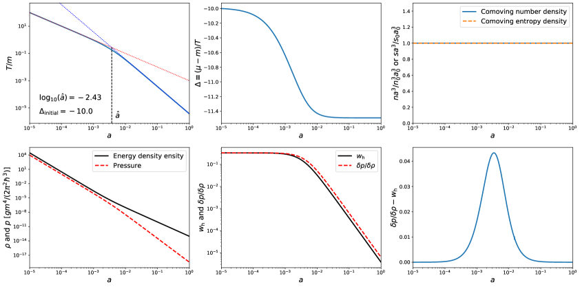
Figure 1: Some solutions to Eqs. (A.17) with $\lim\limits_{x\rightarrow 0}\frac{a}{x}=10^{-3}$ and $\lim\limits_{x\rightarrow 0}\Delta=-10$ (a classical case). The evolution is computed by requiring the comoving particle number and specific entropy (and hence the comoving entropy density) to remain unchanged, which is verified and shown in the upper right panel. The other panels are: the ratio between the temperature and the particle mass $x\equiv T/m$ (upper left), the ratio between the effective chemical potential and the temperature $\Delta\equiv(\mu-m)/T$ (upper middle), energy density $\rho_{\rm{h}}$ and pressure $p_{\rm{h}}$ (lower left), the equation-of-state parameter $w_{\rm{h}}\equiv p_{\rm{h}}/\rho_{\rm{h}}$ and the adiabatic sound speed $c_{\rm{s,h}}^{2}\equiv\delta p_{\rm{h}}/\delta\rho_{\rm{h}}$ (lower middle) and the difference between them (lower right). Different initial values of $\lim\limits_{x\rightarrow 0}\frac{a}{x}$ only horizontally shift the evolution. As long as $\Delta_{\rm{ini}}\leq 0$, the characteristics of the evolution (transition width and transition scale factor) only weakly depend on quantum statistics, which will be shown in Sec. 2.2.

In Figure 1 we show an example of a solution of all the background variables as well as the adiabatic sound speed. In that example, we set $\lim\limits_{x\rightarrow 0}\frac{a}{x}=10^{-3}$ and $\Delta_{\rm{ini}}\equiv\lim\limits_{x\rightarrow 0}\Delta=-10$ corresponding to a classical case since $\Delta\ll-1$. The evolution of the temperature is shown in the upper left panel of Figure 1 along with its asymptotic behavior at the relativistic and nonrelativistic limits. As expected, the temperature of the hidden dark matter (and $1/x$) drops initially as $1/a$ in the relativistic phase (when $x\rightarrow 0$) and then as $1/a^{2}$ in the nonrelativisitc phase (when $x\rightarrow\infty$). The value of $\Delta$ changes from one constant to another constant, which is shown in the upper middle panel; see Appendix A for more discussion. We find that as long as $\Delta_{\rm{ini}}\leq 0$, $\Delta$ is always dropping regardless of the initial conditions or whether the hidden dark matter is a fermion or boson. This means that quantum statistical effects will be less significant after the transition. For bosons in the hidden dark matter scenario, a Bose-Einstein condensation would never take place at the background level if $\Delta_{\rm{ini}}<0$. The drop of $\Delta$ can be calculated analytically; see Eq. (A.16). It is always finite and approaching a constant when $\Delta_{\rm{ini}}\ll-1$. It only weakly depends on $\Delta_{\rm{ini}}$ and whether the HiDM is a fermion or boson when $\Delta\gtrsim-1$. We investigate such a $\Delta_{\rm{ini}}$ dependence in Sec. C. To verify our solutions, the comoving number density and comoving entropy density are shown in the upper right panel. Both of them are constant, as expected. Shown in the lower left panel are the energy density and the pressure. The energy density first drops as $1/a^{4}$ (as radiation) and then as $1/a^{3}$ (behaving as the usual cold dark matter). The pressure first follows the energy density and drops as $1/a^{4}$ and then as $1/a^{5}$. The equation-of-state parameter $w_{\rm{h}}\equiv p_{\rm{h}}/\rho_{\rm{h}}$, as shown in the lower middle panel, exhibits a smooth transition.

2.1.2 Background evolution II: free-streaming case

If the hidden dark matter becomes free streaming before the relativistic-to-nonrelativistic transition, its background-level physical momentum distribution at an arbitrary $a$ is given by [73]

$$f_{\rm{fs}}(p;\,\tilde{T}_{0},a)=\frac{g}{2\pi^{2}\hbar^{3}}\frac{p^{2}}{\exp(pa/\tilde{T}_{0}-\Delta_{\rm ini})\pm 1}\,.$$ (2.2)

In the above equation, $\tilde{T}_{0}\equiv T_{\rm{fs}}a_{\rm{fs}}$ where $T_{\rm{fs}}$ and $a_{\rm{fs}}$ are the dark matter temperature and scale factor at the time when HiDM became free-streaming. We have ignored the term $ma_{\rm{fs}}$ in the above distribution (compared to Eq. (20) in [73]). This is because the hidden dark matter becomes a free stream when they were still relativistic and $\tilde{T}_{0}\gg ma_{\rm{fs}}$; the momenta $pa$ around $\tilde{T}_{0}$ dominate the distribution and they are much larger than $ma_{\rm{fs}}$. In this case, its comoving number density is also conserved. And since the comoving momentum distribution is not changing with time, the comoving entropy is automatically conserved.

When $\Delta_{\rm ini}=0$, the free-stream case recovers the WDM scenario. In this work, we shall show that the free-streaming case actually behaves very similarly to the equilibrium case in both the background evolution and perturbations.

Given the above distribution Eq. (2.2), the energy density and pressure at an arbitrary $a$ can be calculated. We find that the background evolution as derived from Eq. (2.2) is very similar to that of the equilibrium case. In Figure 2 we show a comparison of energy density, equation-of-state parameter, and the nonrelativistic momentum distribution between the free-streaming case and the equilibrium case, taking a fermionic hidden dark matter as an example. Starting from the same mass-to-temperature ratio, the energy densities (left panel) in the two cases only differ from each other by less than $0.5\%$ at all times. The nonrelativistic momentum distributions (right panel) are quite different, but they give a similar velocity dispersion with a fractional difference of only $3\%$.

Since the background evolution in the free-streaming case is similar to that of the equilibrium case, we will use the equilibrium case at the background level as a case study to investigate the constraints on the HiDM model and to identify the most promising regimes in cosmology and astrophysics in which to set the most powerful constraint on this class of HiDM models. Constraints should be only slightly different between different cases. We will however distinguish them at the perturbation level; see Sec. 3.

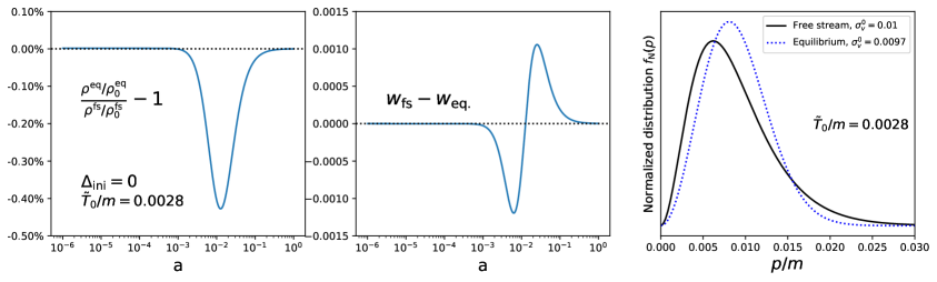
Figure 2: A comparison between the free-streaming case and the equilibrium case. In this example, we consider a fermionic hidden dark matter with $\Delta_{\rm{ini}}=0$. In both cases, the hidden dark matter has $\tilde{T}_{0}/m=0.0028$ where $\tilde{T}_{0}$ is the temperature today in the massless limit. The energy densities in the two cases (left panel) only differ from each other by less than $0.5\%$ at all times. The equation-of-state parameters (middle panel) are close to each other as well. The two nonrelativistic momentum distributions today (right panel) are different, but their velocity dispersions only differ from each other by $3\%$.

2.2 A universal approximation to numerical solutions

It is beneficial to have a good parameterized function to approximate the numerical solution of the background evolution. This can not only simplify and speed up the parameter inference process but also usually allow us to identify some properties that characterize the evolution. We find that the following parameterized functions can very well approximate the evolution of the energy density $\rho_{\rm{h}}$, the equation-of-state parameter $w_{\rm{h}}$, and the squared adiabatic sound speed $c_{\rm{s}}^{2}$ for all cases in the HiDM model:

$$\rho_{\rm{h}} =\frac{\Omega_{\rm{h}}\rho_{\rm{c}}^{0}}{a^{4}}\Big{[}\frac{a^{n_{w}}+(a_{\rm{T}}^{w})^{n_{w}}}{1+(a_{\rm{T}}^{w})^{n_{w}}}\Big{]}^{\frac{1}{n_{w}}}\,,$$ (2.3)

$$w_{\rm{h}} =\frac{1}{3}\frac{(a_{\rm{T}}^{w})^{n_{w}}}{a^{n_{w}}+(a_{\rm{T}}^{w})^{n_{w}}}\,,$$ (2.4)

$$c_{\rm{s}}^{2} =\frac{1}{3}\frac{(a_{\rm{T}}^{c_{\rm{s}}^{2}})^{n_{c_{\rm{s}}^{2}}}}{a^{n_{c_{\rm{s}}^{2}}}+(a_{\rm{T}}^{c_{\rm{s}}^{2}})^{n_{c_{\rm{s}}^{2}}}}\,,$$ (2.5)

where $\rho_{\rm{c}}$ is today’s critical energy density. The transition indices $n_{w}$ and $n_{c_{\rm{s}}^{2}}$ quantify the width in $\ln a$ of the relativistic-to-nonrelativistic transitions of $w_{\rm{h}}$ and $c_{\rm{s}}^{2}$, respectively. The larger the transition index, the sharper the transition. The transition scale factors $a_{\rm{T}}^{w}$ and $a_{\rm{T}}^{c_{\rm{s}}^{2}}$ roughly represent the position in $a$ of the transitions of $w_{\rm{h}}$ and $c_{\rm{s}}^{2}$, respectively. Both $w_{\rm{h}}$ and $c_{\rm{s}}^{2}$ start with $1/3$ and transition to $0$. Note that the functional form of $\rho_{\rm{h}}$ is consistently obtained from the above parameterized $w_{\rm{h}}$ according to $d(\rho_{\rm{h}}a^{3})=-w_{\rm{h}}\rho_{\rm{h}}d(a^{3})$. For a better approximation to the numerical result of $c_{\rm{s}}^{2}$, we use a separate parameterized function [Eq. (2.5)] to fit the evolution of $c_{\rm{s}}^{2}$, rather than calculating it using $dp/d\rho$. More discussions on the above fitting functions and the fitting process can be found in Appendix B.1. In Table 2 we show all the transition parameters ($\delta_{w}^{a}$, $n_{w}$, $\delta_{c_{\rm{s}}^{2}}$, $n_{c_{\rm{s}}^{2}}$) along with other useful quantities (defined later) such as $\alpha_{(w,c_{\rm{s}}^{2})}$ [see Eq. (2.6)], $C$ [see Eqs. (2.7)-(2.9)] and $\Delta_{\rm{ch}}\equiv\Delta_{\rm{f}}-\Delta_{\rm{ini}}$.

We note that the motivation to use these prameterizatized functions (Eqs. (2.3) to (2.5)) is to approximate the evolution of those quantities in the sense that they can closely represent cosmological and observables studied in this work. The evolution of the density is more physically related to cosmological observables than the equation of state. Thus, we directly use the parameterized density evolution Eq. (2.4) to fit the numerical result, instead of the parameterized equation of state. Particular attention needs to be paid to Eq. (2.4). This is because, while Eq. (2.4) can be used to well capture the effects of hidden DM at cosmological scales, it does not represent a correct late-time evolution of the equation of state, which would drop as $\propto 1/a^{2}$ instead of $\propto 1/a^{n_{w}}$. For completeness, a better approximation that correctly captures the late-time temperature evolution shall be given in Eq. (2.8). Similarly, the parameterized adiabatic sound speed Eq. (2.5) does not represent a correct late-time evolution either. But it approximates the relativistic-to-nonrelativistic transition very well and using it can closely reproduce the quantities relevant in cosmological observations, such as the suppression scale in the matter power spectrum discussed in Sec. 5.

Other forms of parameterization can be found in the literature. For example, Ref. [64] uses $w(a)=\frac{1}{3}(1+(a/a_{\rm{T}})^{2p})^{-\frac{1}{p}}$; also see Ref. [74]. While these forms also represent the transition of the equation of state and can correctly represent a late-time behavior, the advantage of our parameterization is that an analytic form of $\rho_{\rm{h}}(a)$ can be obtained. This, as mentioned, allows us to directly fit the parameterized function to the numerical result of the density that is more directly related to observables. Another form adopted in Ref. [75], $w=\frac{1}{6}\big{[}1-\tanh(\frac{a-a_{*}}{\Delta})\big{]}$, does not work in our case. This is because, under this parameterization, $w$ would either exhibit a very sharp transition (e.g., when $\Delta/a_{*}=0.1$) or not start with $1/3$ (e.g., when $\Delta/a_{*}=1$).

	Equilibrium			Free-Streaming
	$\Delta_{\rm{ini}}\ll-1$	$\Delta_{\rm{ini}}=0$, F	$\Delta_{\rm{ini}}=0$, B	$\Delta_{\rm{ini}}\ll-1$	$\Delta_{\rm{ini}}=0$, F	$\Delta_{\rm{ini}}=0$, B
$\delta_{w}^{a}$	$-$0.0930	$-$0.0948	$-$0.0848	N/A	N/A	N/A
$n_{w}$	1.8442	1.8539	1.8197	1.8169	1.8367	1.7838
$\delta_{c_{\rm{s}}^{2}}^{a}$	0.0346	0.0320	0.0440	N/A	N/A	N/A
$n_{c_{\rm{s}}^{2}}$	1.8707	1.8820	1.8463	1.8418	1.8591	1.7993
$\alpha_{w}$	3.0002	3.1529	2.6942	3.0003	3.1515	2.7013
$\alpha_{c_{\rm{s}}^{2}}$	4.0208	4.2217	3.6214	4.0030	4.2082	3.6188
$\delta_{c_{\rm{s}}^{2}}^{a}-\delta_{w}^{a}$	0.1275	0.1268	0.1288	N/A	N/A	N/A
$C$	3.7120	3.9203	3.2802	N/A	N/A	N/A
$\Delta_{\rm{ch}}$	$-1.5$	-1.6202	-1.2451	N/A	N/A	N/A

Table 2: Summary of the transition parameters as well as $\alpha_{(w,c_{\rm{s}}^{2})}$, $C$ and $\Delta_{\rm{ch}}$. The coefficient $\alpha_{(w,c_{\rm{s}}^{2})}$ is defined in Eq. (2.6) and $C$ is defined via Eqs. (2.7) and (2.8). The change of $\Delta$ is defined as $\Delta_{\rm{ch}}\equiv\Delta_{\rm{f}}-\Delta_{\rm{ini}}$. The four transition parameters ($\delta_{w}^{a}$, $n_{w}$, $\delta_{c_{\rm{s}}^{2}}^{a}$ and $n_{c_{\rm{s}}^{2}}$) are the best-fit parameters of the approximations to $\rho_{\rm{h}}$ and $c_{\rm{s}}^{2}$. The fitting functions are Eq. (2.3) for $\rho_{\rm{h}}$ and Eq. (2.5) for $\delta p_{\rm{h}}/\delta\rho_{\rm{h}}$, and $\delta_{a}^{(w,c_{\rm{s}}^{2})}\equiv\log_{10}a_{\rm{T}}^{(w,c_{\rm{s}}^{2})}-\log_{10}\hat{a}$. In the equilibrium case, the classical limits ($\Delta_{\rm ini}\ll-1$) of $C$ and all fitting parameters are given in the second column. A fermion (boson) case with $\Delta_{\rm{ini}}=0$ is shown in the third (fourth) column. “F” and “B” stand for fermion and boson. The corresponding free-streaming cases are shown in the last three columns. In the rest of this work we will use the transition parameters at the classical equilibrium limit to study impacts on cosmological observations and parameter estimations; see Appendix C for more discussions about the phenomenologically weak dependence on different cases. Values of $C$ and $\Delta_{\rm{ch}}$ are derived analytically [see Eq. (A.16) and Eq. (2.9)] and verified by numerical results. In particular, the value of $C=3.712$ in classical limit in the equilibrium case corresponds to $\big{(}\frac{8}{\pi}\big{)}^{\frac{1}{3}}\exp(1)$; see the discussion in Sec. B.2.

2.3 Remarks on the transition parameters and the temperature evolution

Both $a_{\rm{T}}^{w}$ and $a_{\rm{T}}^{c_{\rm{s}}^{2}}$ are proportional to $\tilde{T}_{0}/m$, where $\tilde{T}_{0}$ is the temperature the HiDM would have today if the temperature continued to drop as $1/a$; see the orange dotted line in the upper left panel of Figure 1. We define two proportionality coefficients as

$$\alpha_{w}=\frac{a_{\rm{T}}^{w}}{\tilde{T}_{0}/m}\,,~{}~{}~{}~{}\textrm{and}~{}~{}~{}~{}~{}\alpha_{c_{\rm{s}}^{2}}=\frac{a_{\rm{T}}^{c_{\rm{s}}^{2}}}{\tilde{T}_{0}/m}\,.$$ (2.6)

These two coefficients are slightly different in different cases and can be determined after numerically solving the background evolution and obtaining the best-fit parameters.

For the equilibrium case, we can define a characteristic scale factor $\hat{a}$, which is close to the two transition scale $a_{\rm{T}}$’s defined above but has certain advantages for the study of the temperature evolution. This $\hat{a}$ is defined as follows. The mass-to-temperature ratio $x$ goes as $a$ at early times when $x\ll 1$ and as $a^{2}$ at late times when $x\gg 1$. Such asymptotically relativistic and nonrelativistic behaviors are shown by the dotted lines in the upper left panel of Figure 1 where the reciprocal – the temperature-to-mass ratio $1/x$ – is plotted. We define $\hat{a}$ as the scale factor where the two asymptotic lines meet so that the two limits can be written as

$$\lim_{x\rightarrow 0}x =C\frac{a}{\hat{a}}\,,$$ (2.7)

$$\lim_{x\rightarrow\infty}x =C\frac{a^{2}}{\hat{a}^{2}}\,\,,$$ (2.8)

where $C$ is a constant determined by $\Delta_{\rm{ini}}$ and statistics, and it can be calculated analytically as

$$C=\frac{2}{\pi^{1/3}}\Big{[}\frac{f_{3}^{\mp}(\Delta_{\rm{ini}})}{f_{3/2}^{\mp}(\Delta_{\rm{f}})}\Big{]}^{\frac{2}{3}}\exp\big{(}-\frac{2}{3}\Delta_{\rm{ch}}\big{)}\,,$$ (2.9)

where $\Delta_{\rm{ch}}$ can be derived analytically with Eq. (A.16) and the function $f_{s}^{\mp}$ defined in Eq. (A.10) is of the order unity. One can use the above equations to infer the temperature in the nonrelativistic limit when given the temperature in the relativistic limit. Note that there are small differences between the two transition scale factors $a_{\rm{T}}$ and the characteristic scale factor $\hat{a}$. Also, as we shall show, the differences among these three scale factors are independent of the initial $x_{\rm ini}$ and vary only slightly for different cases in our $\Lambda$HiDM model. To isolate the dependence on the initial $x_{\rm ini}$, we quantify the differences among the three scale factors on a log10 scale and define $\delta_{a}^{w}\equiv\log_{10}a_{\rm{T}}^{w}-\log_{10}\hat{a}$ and $\delta_{a}^{c_{\rm{s}}^{2}}\equiv\log_{10}a_{\rm{T}}^{c_{\rm{s}}^{2}}-\log_{10}\hat{a}$.

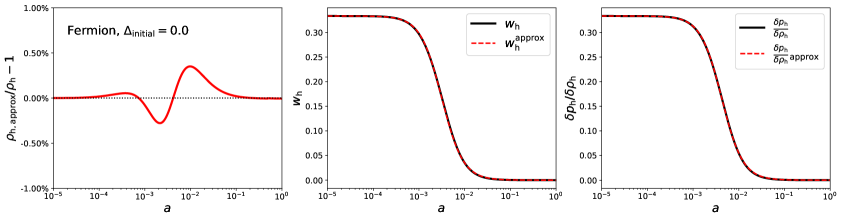
Figure 3: Comparison between the numerical solutions and approximations for a fermion case with $\Delta_{\rm{ini}}=0$. The best-fit parameters for this case are listed in the second column of Table 2. Left: the fractional difference between the numerical solution of $\rho_{\rm{h}}$ and its best-fit approximation. The fitting function is Eq. (2.3). The fractional difference is within $0.5\%$ at all times. Middle: the numerical solution of $w_{\rm{h}}$ (solid black) and its approximation [dashed red, calculated with Eq. (2.4)]. Right: $\delta p_{\rm{h}}/\delta\rho_{\rm{h}}$ and its approximation. The numerical solution and the approximation match very well in all cases.

Then, given $\hat{a}$, the four transition parameters, $\delta_{a}^{w}$, $n_{w}$, $\delta_{a}^{c_{\rm{s}}^{2}}$ and $n_{c_{\rm{s}}^{2}}$, determine the evolution as parameterized by Eqs. (2.3)-(2.5). We fit the parameterized functions to the numerical solutions of $\rho_{\rm{h}}$ and $c_{\rm{s}}^{2}$ to find the best-fit transition parameters. The fitting process is detailed in Appendices B.2 and B.3. We show the best-fit transition parameters along with other useful constants in Table 2. We show in Figure 3 an example of a comparison between the fitting functions and the numerical solutions for a fermionic HiDM model with $\Delta_{\rm{ini}}=0$ in equilibrium. The fractional difference in the energy density between the approximation and the numerical solution is within about $0.5\%$ at all times. The approximations to the equation-of-state parameter and the adiabatic sound speed are also very good. We include another example for the free-streaming case in Appendix B.3. These conclusions about the approximation and the numerical solution apply to all cases we consider in this work.

From Table 2 we can see that different cases have different transition parameters. This means that starting with the same mass-to-temperature ratio, the transition position and width (in $a$) are in principle different. However, in practice, they are very close, which implies that the observational effects are similar for all cases we consider. Indeed, for the background evolution, we can see from our approximations [Eq. (2.3)-(2.5)] that the most relevant properties of the evolution are the transition position, the transition gap between $w_{\rm{h}}$ and $c_{\rm{s}}^{2}$, and the width of the transition. While the latter two are very similar for all cases [see the rows of $n_{w}$, $n_{c_{\rm{s}}^{2}}$ and ($\delta_{c_{\rm{s}}^{2}}^{a}-\delta_{w}^{a}$) in Table 2], the transition positions in different cases can be brought to agreement by changing the initial mass-to-temperature ratios. See Appendix C for more discussion. These results show that it is justified to take the background evolution in this classical case as our representative case to study the impacts on cosmological observables and their associated constraints. We will however treat the equilibrium case and free-streaming cases differently at the perturbation level; see Sec. 3.2.

The background evolution in our representative case (the classical equilibrium case) only depends on the initial mass-to-temperature ratio of the hidden dark matter, or, equivalently, the characteristic scale factor $\hat{a}$. We define the following parameter,

$$R^{\rm{T}}_{\rm{eq}}\equiv\frac{\hat{a}}{a_{\rm{eq}}}\,,$$ (2.10)

where $a_{\rm{eq}}=\frac{4.15\times 10^{-5}}{\Omega_{\rm{m}}h^{2}}$ is the scale factor at matter-radiation equality in the standard CDM case. With this definition, $R^{\rm{T}}_{\rm{eq}}<1$ means that the transition happened before the standard matter-radiation equality. The standard cold dark matter case corresponds to $R^{\rm{T}}_{\rm{eq}}=0$. All the transition parameters ($\delta_{a}^{w}$, $n_{w}$, $\delta_{a}^{c_{\rm{s}}^{2}}$ and $n_{c_{\rm{s}}^{2}}$) are taken to be their classical limits shown in the first column in Table 2.

For the usual WDM scenario, the relativisitic-to-nonrelativistic transition time (parameterized by $R_{\rm{eq}}^{\rm{T}}$) can be determined from by the dark matter density fraction today and the particle mass [49, 50]. In our HiDM scenario, the relation between particle mass and the transition time is modified and given by

$$\Omega_{\rm{dm}}h^{2}=g\,\xi(\Delta_{\rm{ini}})e^{\Delta_{\rm{ini}}}\left(\frac{m}{6.4\,\rm{keV}}\right)^{4}\left(\frac{R_{\rm{eq}}^{\rm{T}}}{10^{-4}}\right)^{3}\,$$ (2.11)

where $\xi(\Delta_{\rm{ini}})\equiv\frac{f_{3}^{\mp}(\Delta_{\rm{ini}})}{(C/3.712)^{3}}$ is of the order unity. Due to the factor of $e^{\Delta_{\rm{ini}}}$, for a given mass of dark matter, a later transition (larger $R_{\rm{eq}}^{\rm{T}}$) is required for a lower value of $\Delta_{\rm{ini}}$ to account for the observed dark matter abundance. As we shall see, observations put upper bounds on $R^{\rm{T}}_{\rm{eq}}$. In the WDM scenario with $\Delta_{\rm ini}=0$, an upper bound on $R^{\rm{T}}_{\rm{eq}}$ corresponds to a lower bound on the particle mass. In the HiDM scenario, the corresponding lower bounds on the particle mass become even stronger when $\Delta_{\rm ini}<0$.

Now, the evolution of the hidden dark matter model with conservation of comoving number density and comoving entropy can be well parameterized by only two parameters: $\Omega_{\rm{h}}$ and $R^{\rm{T}}_{\rm{eq}}$. Therefore, we have only one additional parameter compared to the standard $\Lambda$CDM model: $R_{\rm{eq}}^{\rm{T}}$. This one-parameter family of dark matter models is similar to that of the warm dark matter proposed in Ref. [49] but ours is more generalized, allowing different quantum statistics, initial chemical potential, and dark matter models that are either in their own equilibrium or free streaming. The conclusions about the impacts on cosmological observations and parameter estimations presented later in this work are independent of the mass, the intrinsic degrees of freedom, or the background expansion. Additionally, they are fairly insensitive to whether the dark matter is free streaming or in thermal equilibrium, and whether it is composed of fermions or bosons (as long as $\Delta_{\rm ini}\leq 0$).

2.4 Constraints from Big Bang Nucleosynthesis element abundance

If dark matter were relativistic during BBN, the presence of extra relativistic degrees of freedom would have caused the expansion of the universe to be faster, altering the primordial element abundance. Abundance observations of, e.g., primordial deuterium and helium have independently put a constraint on the extra radiation energy [76, 77]. This puts a constraint on the transition time for HiDM and thus an upper bound on $R^{\rm{T}}_{\rm{eq}}$.

In Appendix D we show that $R^{\rm{T}}_{\rm{eq}}$ is related to $\Delta N_{\rm{eff}}$, which parameterizes the extra radiation energy density at BBN. When $\hat{a}$ is sufficiently small, we have (see Appendix for discussion),

$$R_{\rm{eq}}^{\rm{T}}=0.28\times\frac{\Omega_{\rm{m}}\Omega_{\gamma}}{\Omega_{\rm{dm}}\Omega_{\rm{rad}}}\Delta N_{\rm{eff}}\,,$$ (2.12)

where $\Omega_{\rm{m}}$, $\Omega_{\rm{dm}}$, $\Omega_{\gamma}$ and $\Omega_{\rm{rad}}$ are today’s density parameters of matter, dark matter, photons and total radiation. We however emphasize that our $\Lambda$HiDM model is not equivalent to an $\Delta N_{\rm{eff}}$-$\Lambda$CDM model when other cosmological and astrophysical observations are concerned. The effects on different observations will be analyzed individually. As we shall see, other cosmological and astrophysical constraints on $R_{\rm{eq}}^{\rm{T}}$ are much stronger than the constraint from BBN; we nonetheless provide a rough estimate of the BBN constraint here. By fixing all $\Omega$’s to the mean values given in Planck 2018 [5] and conservatively taking the upper bound $\Delta N_{\rm{eff}}<1$ [77], we have the upper bound of $R_{\rm{eq}}^{\rm{T}}$ constrained by BBN,

$$R_{\rm{eq}}^{\rm{T}}\lesssim 0.2\,.$$ (2.13)

We have ignored the uncertainties of all $\Omega$’s, as they are sub-dominant. Compared to the other constraints we estimate for the $\Lambda$HiDM model, this BBN constraint is the weakest.

3 Scalar perturbations of the hidden dark matter

The hidden dark matter scenario has interesting phenomenology at the perturbation level. In the standard CDM scenario, the dark matter overdensity always grows (in the synchronous gauge) due to gravitational instability. If the hidden dark matter were relativistic, the overdensity would oscillate. If the relativistic-to-nonrelativistic transition occurs late enough, this would lead to an observable suppression of small-scale structure due to such oscillations. In this section, we first describe the perturbation equations and the initial conditions of the hidden dark matter scenario. We mainly follow the notation in [78], and we use the synchronous gauge. In this work, we will only consider scalar mode perturbations with adiabatic initial conditions and zero spatial curvature.

3.1 Perturbations in standard CDM

In the standard cold dark matter scenario, the velocity potential of dark matter is constant. This allows us to make a gauge transformation to make the velocity potential vanish and fix the residual degree of freedom in synchronous gauge [79, CH. 5]. When the velocity potential vanishes, the fluid dynamics of the cold dark matter is simply given by

$$\delta_{\rm{c}}^{\prime}=-h_{\rm{s}}^{\prime}/2\,,$$ (3.1)

where ^′ denotes the derivative with respect to the conformal time $\eta$, and $h_{\rm{s}}$ is one of the gravitational variables in synchronous gauge. Another relevant differential equation is that of the other synchronous gauge gravitational variable $\eta_{\rm{s}}$ (to be distinguished from the conformal time $\eta$) [78],

$$k\eta_{\rm{s}}^{\prime}=4\pi Ga^{2}\sum\rho_{i}q_{i}\,,$$ (3.2)

where $k$ is the comoving wavenumber and $q_{i}$ is the heat flux of the $i$th species (which vanishes for cold dark matter). The adiabatic initial condition for $\delta_{\rm{c}}$ to next-to-leading order is

$$\delta_{\rm{c}}(k\eta\ll 1)=\mathcal{R}_{k}\Big{[}-\frac{1}{4}k^{2}\eta^{2}+\frac{1}{20}\frac{\Omega_{\rm{m}}\mathcal{H}_{0}}{\sqrt{\Omega_{\rm{R}}}}k^{2}\eta^{3}\Big{]}\,,$$ (3.3)

where $\delta_{\rm{c}}\equiv\delta\rho_{\rm{c}}/\bar{\rho}_{\rm{c}}$, $\mathcal{R}_{k}$ is the primordial curvature perturbation, $\mathcal{H}_{0}$ is the conformal Hubble constant, and $\Omega_{\rm{m}}$ and $\Omega_{\rm{R}}$ are the matter and radiation energy fraction today.

3.2 Perturbations of the hidden dark matter

The major changes to the perturbation equations are the fluid dynamics of the hidden dark matter. In the hidden dark matter scenario, $w_{\rm{h}}$ is not negligible, and the velocity potential of dark matter is not a constant. Therefore, we cannot simply use a gauge transformation to make the dark matter velocity potential vanish; we must include the bulk velocity of the HiDM in its fluid dynamics. Fortunately, if the relativistic-to-nonrelativistic transition happened much earlier than last scattering, as it should, the velocity potential can be considered constant long before last scattering. Then, the bulk velocity should have decayed to a negligible level, which means that during and after last scattering, the residual gauge degree of freedom is unimportant, and we do not have to perform a gauge transformation to fix the synchronous gauge.

The equations of fluid dynamics for hidden dark matter in a general case are [78]

$$\delta_{\rm{h}}^{\prime} =-kq_{\rm{h}}-(1+w_{\rm{h}})h_{\rm{s}}^{\prime}/2+3\mathcal{H}(w_{\rm{h}}-\frac{\delta p_{\rm{h}}}{\delta\rho_{\rm{h}}})\delta_{\rm{h}}\,,$$ (3.4)

$$q_{\rm{h}}^{\prime} =(3w_{\rm{h}}-1)\mathcal{H}q_{\rm{h}}+k\frac{\delta p_{\rm{h}}}{\delta\rho_{\rm{h}}}\delta_{\rm{h}}-\frac{2}{3}w_{\rm{h}}k\pi_{\rm{h}}\,,$$ (3.5)

where the subscript “h” means “hidden”, $q_{\rm{h}}$ is the heat flux, $w_{\rm{h}}$ the equation-of-state parameter, $\delta p_{\rm{h}}/\delta\rho_{\rm{h}}$ the adiabatic sound speed squared (discussed in Sec. 2), and $\pi_{\rm{h}}$ the scalar anisotropic stress . Due to the nonvanishing $q_{\rm{h}}$, there will be an additional source term in the differential equation of $\eta_{\rm{s}}$, i.e.,

$$k\eta_{\rm{s}}^{\prime}=4\pi Ga^{2}\Big{(}\sum\rho_{i}q_{i}+\rho_{\rm{h}}q_{\rm{h}}\Big{)}\,,$$ (3.6)

where $i$ goes through all contents except for the hidden dark matter.

The anisotropic stress is another (small) difference between the equilibrium case and the free-streaming case. Initially, $\pi_{\rm{h}}=0$ for both cases. When there is a momentum anisotropy in the phase-space distribution, the scalar anisotropic stress is finite and manifests as off-diagonal components in the perturbed stress-energy tensor, i.e., $\delta T_{ij}=a^{2}\partial_{i}\partial_{j}\pi_{\rm{h}}$ where $\partial_{i}$ is the spatial coordinate partial derivative. For the equilibrium case, the phase-space distribution remains isotropic, therefore $\pi_{\rm{h}}$ vanishes at all times. For the free-streaming case, however, even if the phase-space distribution starts out isotropic, the stream from a hotter place will be different than that from a colder place, resulting in a finite anisotropic stress.

Following Ref. [64], the dynamics of $\pi_{\rm{h}}$ can be approximately captured by the following parameterized equation,

$$\pi_{\rm{h}}^{\prime}=-3\mathcal{H}\pi_{\rm{h}}+\frac{4c_{\rm{vis}}^{2}}{w_{\rm{h}}}\big{(}\frac{kq_{\rm{h}}}{1+w_{\rm{h}}}+h_{\rm{s}}^{\prime}/2+3\eta_{\rm{s}}^{\prime}\big{)}\,,$$ (3.7)

where $c_{\rm{vis}}^{2}$ is a viscosity parameter. We model the viscosity term with two parameterizations: (1) $c_{\rm{vis}}^{2}=0$, which corresponds to a situation in which there is some elastic self-interaction sufficient to keep the perturbed distribution in equilibrium, so that $\pi_{\rm{h}}=0$ at all times, consistent with the above discussion (recalling that initially $\pi_{\rm{h}}=0$); and (2) $c_{\rm{vis}}^{2}=w_{\rm{h}}$, which mimics the free-streaming case and serves as a source for the anisotropic stress [64]. For a more precise treatment of the second case, one should consider higher-moment-hierarchy Boltzmann equations [73, 80].

We assume that perturbations in the hidden dark matter scenario are seeded by adiabatic initial conditions. Note that dark matter isocurvature modes can naturally exist when the dark matter does not begin in thermal contact with the Standard Model sector; see e.g. Ref. [81]. However, the primordial isocurvature component has been tightly constrained by Planck [82], so we will assume adiabatic initial conditions. We will see that since the hidden dark matter is initially relativistic, the adiabatic initial conditions of the density perturbations of the hidden dark matter are different from the standard case and are now the same as those of photons:

$$\delta_{\rm{h}}(k\eta\ll 1)=\mathcal{R}_{k}\Big{[}-\frac{1}{3}k^{2}\eta^{2}+\frac{1}{15}\frac{\Omega_{\rm{b}}\mathcal{H}_{0}k^{2}\eta^{3}}{\sqrt{\Omega_{\rm{R}}+\hat{a}\,\Omega_{\rm{h}}}}\Big{]}\,.$$ (3.8)

Note the coefficient of the next-to-leading order term above is now different from that in Eq. (3.3) because the hidden dark matter in this case initially behaves as a type of radiation. The next-to-leading order approximation of the initial conditions of other variables also needs to be changed consistently. We let the initial conditions of $q_{\rm{h}}$ also equal those of the photon heat flux, i.e.,

$$q_{\rm{h}}(k\eta\ll 1)=-\frac{\mathcal{R}_{k}}{27}k^{3}\eta^{3}\,,$$ (3.9)

but we find that results are insensitive to this.

Our $\Lambda$HiDM model consists of $7$ parameters: $6$ standard $\Lambda$CDM parameters plus $R^{\rm{T}}_{\rm{eq}}$. We do two separate analyses, one with viscosity and the other without. We implement the background and perturbation equations by modifying camb [83], and perform parameter estimations using cosmomc [84].

4 Large scales: impacts on CMB power spectra and constraints from Planck

The effects of HiDM at the perturbation level are described by the modified transfer functions, which are the growth of perturbations at a given time and scale with respect to their initial conditions. In this section, we investigate the impacts of HiDM on the transfer functions of cosmological perturbations and the CMB power spectra and use the publicly available Planck 2018 baseline data ($TT$, $TE$, and $EE$ power spectra) to set constraints on the additional model parameter $R^{\rm{T}}_{\rm{eq}}$.

Related constraints can be found in the literature: e.g, the CMB or joint cosmological constraints on a constant DM equation of state [85, 86], binned equation of state [87], ballistic dark matter [75], or a reduced relativistic dark matter model in which all dark matter particles have the same velocity [71, 72]. In this work, the time evolution of the equation of state is calculated by fully considering the thermal distribution.

4.1 Impacts on the transfer functions

The hidden dark matter being initially relativistic introduces a characteristic scale: a sound horizon of the hidden dark matter, $l_{\rm{s}}\equiv\int c_{\rm{s}}d\eta$, below which matter overdensity perturbations will be smoothed and “suppressed” compared to the standard cold dark matter case. When there is a nonzero viscosity there is another characteristic scale, the viscous scale, $l_{\rm{vis}}\equiv\int c_{\rm{vis}}d\eta$, below which the perturbations will be further suppressed. When $c_{\rm{vis}}^{2}=w_{\rm{h}}$ we have $c_{\rm{vis}}^{2}\leq c_{\rm{s}}^{2}$ (see the bottom middle panel of Figure 1); the viscous scale is similar to but smaller than the sound horizon.

Since $c_{\rm{s}}$ is of the order unity before the transition and zero after, the sound horizon $l_{\rm{s}}$ is similar to the particle horizon at $a=\hat{a}$. Therefore, roughly speaking, a large-scale mode that enters the horizon after $a=\hat{a}$ has a wavelength larger than the sound horizon and experiences nearly no change compared to the standard CDM case. In contrast, a small-scale mode that enters the horizon before $a=\hat{a}$ has a comoving wavelength smaller than the sound horizon. These HiDM overdensity perturbations then oscillate and get suppressed compared to the standard CDM case. This can be seen in Figure 4. By comparing the solid and the dotted lines we can see that, the large-scale (small $k$) perturbation (left panel) evolves the same way as in the CDM case. An intermediate scale (middle panel) that enters the horizon around $a=\hat{a}$ begins to have a significant evolution and suffers from a suppression compared to the CDM case. For an even smaller-scale mode that is still deep inside the horizon before $a=\hat{a}$ (right panel), the dark matter overdensity first oscillates along with the photon overdensity before the relativistic-to-nonrelativistic transition. Around and after the transition, the dark matter oscillation differs from that of the photon, but the oscillation continues until the dark matter bulk velocity becomes too small to affect the growth of large-scale structure. Then, the dark matter overdensity grows due to gravitational instability, but the magnitude by today is much smaller compared to the standard CDM case. Setting a viscosity further suppresses the matter density as we compare the bottom to the top panels in Figure 4.

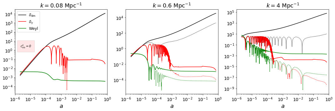
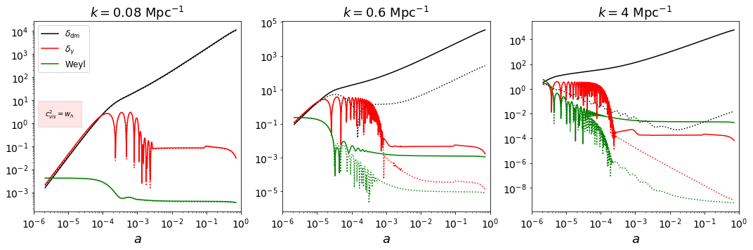
Figure 4: The linear evolution of transfer functions with (top) and without (bottom) a viscosity. Solid lines are in the standard CDM case while dotted lines are the HiDM case. The value of $R_{\rm{eq}}^{\rm{T}}=0.024$ is chosen to be the upper bound at $2\sigma$ as constrained by the Planck 2018 baseline datasets. For a large-scale mode (small $k$) that enters the horizon before $a=a_{\rm{T}}$ on the left, the dark matter overdensity evolves similarly to the standard CDM case. Two small-scale modes are shown on the right. Roughly speaking, when the modes enter the horizon before $a=a_{\rm{T}}$, their wavelengths are smaller than the sound horizon $l_{\rm{s}}$. The dark matter overdensity perturbations then oscillate and get suppressed compared to the standard CDM case. Setting the viscosity even further suppresses the matter density. See the text for detailed discussions.

4.2 Impacts on CMB temperature and polarization power spectra

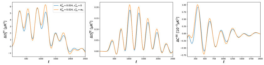
Figure 5: Impacts on CMB power spectra with and without a viscosity. Here the difference between of power spectra in the $\Lambda$HiDM and $\Lambda$CDM models are displayed, and $\mathcal{D}_{\ell}=\ell(\ell+1)C_{\ell}/2\pi$. The value of $R^{\rm{T}}_{\rm{eq}}=0.024$ is chosen to be the $2\sigma$ upper limit as constrained by the Planck 2018 baseline dataset. The viscosity only has a small additional effect on the CMB spectra.

For large-scale perturbations that are relevant to the current CMB baseline observations, there is a connection between the hidden dark matter scenario and the scenario in which a primordial correlated cold dark matter isocurvature mode (CDI) is added to the standard adiabatic initial conditions, as we shall explain. First, for CMB power spectra, most perturbations of interest were still outside the horizon by $a=\hat{a}$. Take $R^{\rm{T}}_{\rm{eq}}=0.01$, for example. Perturbations with a comoving wavenumber smaller than $\hat{k}\equiv\hat{\mathcal{H}}\simeq\frac{0.01}{R^{\rm{T}}_{\rm{eq}}}\,[h\,{\rm{Mpc}}^{-1}]=1\,[h\,{\rm{Mpc}}^{-1}]$ were outside the horizon by $a=\hat{a}$. This range covers most of the perturbations relevant to the current CMB observations, and hence they were still outside the horizon by $a=\hat{a}$. Second, for large scales, the adiabatic solutions of the modified perturbation equations only differ from those of the standard equations by a different $\delta_{\rm{h}}$ (and an additional variable $q_{\rm{h}}$). Let us approximate the transition with a sudden change at $\hat{a}$. Before $\hat{a}$, the dark matter perturbation equation is a relativistic one. The adiabatic solution of $\delta_{\rm{h}}$ when $k\eta\ll 1$ is Eq. (3.8). After $\hat{a}$ the perturbation equations return to the standard ones. Since $k\eta<1$ is still satisfied, Eq. (3.3) would be the adiabatic solution of $\delta_{\rm{h}}$ if it were the standard case. But now $\delta_{\rm{h}}$ is a factor of $4/3$ larger than it would be in the standard case at $a=\hat{a}$. Since solutions of other quantities are unchanged, this extra $1/3$ of the magnitude of $\delta_{\rm{h}}$ serves as a CDI mode. And since it is always $1/3$, this “effective” CDI mode is “fully correlated” with the adiabatic mode. In other words, this hidden dark matter model is another scenario that can produce a CDI mode at large scales without multi-field inflation. The effects on the CMB temperature and polarization spectra are shown in Figure 5.

We emphasize that this is not a situation in which perturbations started with a CDI mode in addition to the adiabatic mode. The perturbations in the hidden dark matter scenario start with purely adiabatic initial conditions, but they are equivalent to the standard perturbations with a CDI mode with a specific functional form of $k$ in addition to the adiabatic mode at (but only at) large scales. Such a degeneracy breaks down at smaller scales where horizon crossings happened before the transition, which will be explored in Sec. 5.

4.3 Constraints from Planck 2018 baseline datasets

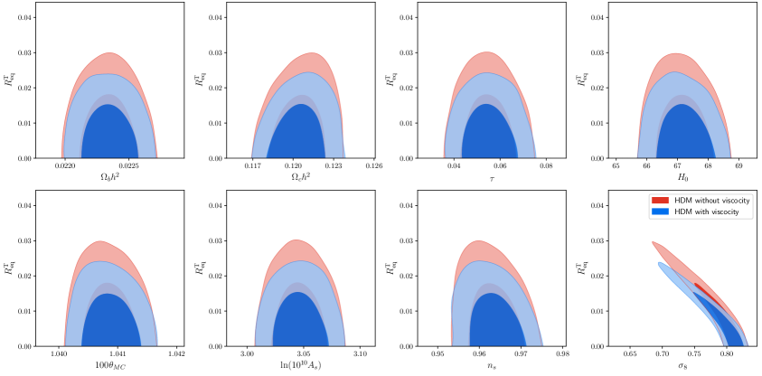
Figure 6: Marginalized constraints on $R^{\rm{T}}_{\rm{eq}}$ versus other standard $\Lambda$CDM model parameters. $R^{\rm{T}}_{\rm{eq}}$ only very weakly correlates with the six base parameters in the $\Lambda$CDM model. Setting the viscosity only slightly tightens the constraint on $R_{\rm{eq}}^{\rm{T}}$. Two important inferred parameters, i.e., $H_{0}$ and $\sigma_{8}$, are shown on the right column. The constraint on $H_{0}$ is not affected, but $\sigma_{8}$ correlates with $R^{\rm{T}}_{\rm{eq}}$. A larger $R^{\rm{T}}_{\rm{eq}}$ leads to a smaller $\sigma_{8}$. It thus might be suspected that the hidden dark matter model can resolve the $\sigma_{8}$ tension. However, as we shall see in Sec. 5, the constraint on $R^{\rm{T}}_{\rm{eq}}$ from Lyman-$\alpha$ forest and smallest halos are so strong that such possibility is eliminated.

In this section, we study the constraints on the transition time from the Planck 2018 baseline datasets. In the previous section, we have shown that for the scales most relevant to CMB observations, there is a connection between the hidden dark matter scenario and an extra CDM isocurvature mode. Planck has tight constraints on the magnitude of isocurvature modes [82]. Before constraining $R^{\rm{T}}_{\rm{eq}}$ with real Planck data, we can roughly estimate its bound from Planck’s constraint on the correlated CDI mode. The upper bound of $\mathcal{P}_{\mathcal{II}}/\mathcal{P}_{\mathcal{RR}}$ for a correlated CDI mode with $n_{\mathcal{II}}=n_{\mathcal{RR}}$ is about $0.001$ at a $2\sigma$ confidence level at $k=0.1$ Mpc^-1 from the publicly released Planck 2018 baseline data [82]. Let us infer the constraint on $R^{\rm{T}}_{\rm{eq}}$ from this. In the standard scenario and in synchronous gauge, the dark matter overdensity fraction $\delta_{\rm{dm}}$ initially grows as $-\frac{1}{4}\mathcal{R}_{k}k^{2}\eta^{2}$ in the adiabatic mode and is a constant $\mathcal{I}_{k}$ in the CDI mode [88]. If these continue to horizon crossing (when $k\eta=1$), the amplitude ratio between $\delta_{\rm{dm}}$ in the two modes would be $\big{|}\frac{\delta_{\rm{dm}}^{\mathcal{I}}(k\eta=1)}{\delta_{\rm{dm}}^{\mathcal{R}}(k\eta=1)}\big{|}=4\big{|}\frac{\mathcal{I}_{k}}{\mathcal{R}_{k}}\big{|}=4\sqrt{\frac{\mathcal{P}_{\mathcal{RR}}(k)}{\mathcal{P}_{\mathcal{II}}(k)}}$. We have followed the notation in Ref. [89] and $\mathcal{P}_{\mathcal{RR}}(k)=\frac{k^{3}}{2\pi^{2}}|\mathcal{R}_{k}|^{2}$, where $|\mathcal{R}_{k}|$ is interpreted as the root mean square of $\mathcal{R}_{k}$. Now, for the largest scales, the hidden dark matter scenario behaves like a standard cold dark matter scenario plus an additional correlated CDI mode, as discussed earlier. Such an equivalent CDI mode has a dark matter overdensity with $1/3$ of the magnitude of that in the standard adiabatic mode at $a=\hat{a}$, i.e., $\delta_{\rm{dm}}^{\mathcal{I}}(\hat{a})/\delta_{\rm{dm}}^{\mathcal{R}}(\hat{a})=1/3$. If the superhorizon evolution was still valid by the time of horizon crossing, the magnitude ratio between this additional isocurvature and the standard adiabatic dark matter perturbations would drop to

$$\left|\frac{\delta_{\rm{dm}}^{\mathcal{I}}(k\eta=1)}{\delta_{\rm{dm}}^{\mathcal{R}}(k\eta=1)}\right|\simeq\frac{1}{3}\frac{k^{2}\hat{\eta}^{2}}{(k\eta=1)^{2}}=\frac{1}{3}k^{2}\hat{\eta}^{2}\simeq\frac{k^{2}a_{\rm{eq}}^{2}}{3\Omega_{\rm{R}}H_{0}^{2}}(R_{\rm{eq}}^{\rm{T}})^{2}\,.$$ (4.1)

In the last equality above, we have used $\hat{\eta}=\frac{\hat{a}}{\sqrt{\Omega_{\rm{R}}H_{0}^{2}}}$ since the is in the radiation dominated era as well as the definition of $R_{\rm eq}^{\rm T}$ (Eq. (2.10)). This means

$$\beta(k) \equiv\frac{\mathcal{P}_{\mathcal{II}}(k)}{\mathcal{P}_{\mathcal{RR}}(k)+{\mathcal{P}_{\mathcal{II}}(k)}}\simeq\frac{\mathcal{P}_{\mathcal{II}}(k)}{\mathcal{P}_{\mathcal{RR}}(k)}=\big{(}\frac{k^{2}\Omega_{\rm{R}}}{12\Omega_{\rm{m}}^{2}H_{0}^{2}}\big{)}^{2}\big{(}R^{\rm{T}}_{\rm{eq}}\big{)}^{4}\,,$$ (4.2)

$${\rm{or}}~{}~{}~{}~{}~{}~{}R^{\rm{T}}_{\rm{eq}} \simeq\frac{1.15\times 10^{-3}}{k/[\rm{Mpc}^{-1}]}\frac{\Omega_{\rm{m}}h^{2}}{\sqrt{\Omega_{\rm{R}}h^{2}}}\beta^{1/4}\,.$$ (4.3)

From the above approximation, we can then use a constraint on $\beta(k)$ to estimate the constraint on $R_{\rm{eq}}$. A subtlety is that from Eq. 4.2 we can see that such an effective CDI mode has a spectral index of $n_{\mathcal{II}}\simeq 5$, since $\mathcal{P}_{\mathcal{II}}(k)\propto k^{4}$ if the adiabatic spectral index $n_{s}^{\mathcal{R}}\simeq 1$. This is different from $n_{\mathcal{II}}=n_{\mathcal{RR}}$ for the special correlated CDI mode considered in the Planck paper [82]. But since such an effective CDI spectrum is blue tilted, the most relevant constraint on $\beta$ given in Ref. [82] is at the small scales. So, we use the upper bound of $\beta<0.001$ ($2\sigma$) given at $k_{\rm{high}}=0.1$ Mpc^-1 to estimate the bound on $R_{\rm{eq}}^{\rm{T}}$. This gives $R_{\rm{eq}}^{\rm{T}}<0.045$ using $\Omega_{\rm{R}}h^{2}=4.157\times 10^{-5}$ and $\Omega_{\rm{m}}h^{2}=0.143$. This is a rough estimate, and we expect the actual constraint on $R_{\rm{eq}}$ from a likelihood analysis to be stronger because Planck probes even smaller scales. Indeed, we performed a likelihood analysis using CosmoMC with our modified camb and found $R^{\rm{T}}_{\rm{eq}}<0.024$ at a $2\sigma$ level. This constraint is about twice as strong as our rough estimate. Some marginalized constraints on $R^{\rm{T}}_{\rm{eq}}$ versus other standard $\Lambda$CDM parameters are shown in Figure 6. From Figure 6 we can also see that while being a little tighter, the constraint on $R^{\rm{T}}_{\rm{eq}}$ is not substantially affected by the setting of viscosity.

We show in Figure 6 the marginalized constraints on $R^{\rm{T}}_{\rm{eq}}$ vs other standard $\Lambda$CDM parameters, with and without a viscosity. We can see that $R^{\rm{T}}_{\rm{eq}}$ only very weakly correlates with the six base parameters in the $\Lambda$CDM model — i.e., $\Omega_{\rm{b}}h^{2}$, $\Omega_{\rm{c}}h^{2}$, $\tau$, $100\theta_{\rm{MC}}$, $\ln(10^{10}A_{s})$ and $n_{s}$ — so varying parameter $R^{\rm{T}}_{\rm{eq}}$ does not affect the constraints on those six standard parameters. We also show on the right column of Figure 6 the constraints on two important derived parameters, $H_{0}$ and $\sigma_{8}$. The constraint on $H_{0}$ is not affected either, but $\sigma_{8}$ correlates with $R^{\rm{T}}_{\rm{eq}}$. A larger $R^{\rm{T}}_{\rm{eq}}$ leads to a smaller $\sigma_{8}$, because of the suppression of the small-scale dark matter perturbations, as discussed in the previous section and shown in Figure 4. The suppressed matter power spectrum is shown in Figure 7. This could suggest that varying $R^{\rm{T}}_{\rm{eq}}$ might resolve the $\sigma_{8}$ tension[90, 7, 8]. But we shall show that the constraint on $R^{\rm{T}}_{\rm{eq}}$ from the Lyman-$\alpha$ forest is about an order of magnitude stronger than that from the CMB, eliminating the possibility for this hidden dark matter to resolve the $\sigma_{8}$ tension.

5 Intermediate scales, impact on the matter power spectrum, and constraints from the Lyman-Alpha forest

We have mentioned in the previous section that the early-time relativistic phase of the hidden dark matter suppresses the small-scale matter power spectrum. This suppression effect is very similar to that in the warm dark matter scenario, where the suppression scale (in that case, the free-streaming scale) is determined by the dark matter mass [69, 50, 35, 91]. However, our hidden dark matter model includes both the equilibrium case (in which the suppression scale is close to the sound horizon) and the free-streaming case. More rigorously, a suppression scale is defined based on the ratio of the suppressed dark matter transfer function to the standard CDM transfer function [50]. Following Ref. [50], we define a suppression scale as the scale at which

$$\frac{P_{\Lambda{\rm{HiDM}}}(k_{\rm{sup}})}{P_{\Lambda{\rm{CDM}}}(k_{\rm{sup}})}=f_{\rm{sup}}\,,$$ (5.1)

where $f_{\rm{sup}}$ is chosen to be $0.1$. This means that at $k=k_{\rm{sup}}$ the power spectrum amplitude is an order of magnitude smaller than that in the standard $\Lambda$CDM case. Numerically, we vary $R^{\rm{T}}_{\rm{eq}}$ and use Eq. (5.1) to evaluate $k_{\rm{sup}}$ and find that $k_{\rm{sup}}$ and $R^{\rm{T}}_{\rm{eq}}$ follow a power law relation,

$$k_{\rm{sup}}=4.1\,{\rm{Mpc}}^{-1}\times\left(\frac{0.001}{R^{\rm{T}}_{\rm{eq}}}\right)^{0.83}\,,$$ (5.2)

where we have used $\Omega_{\rm{m}}h^{2}=0.143$ and $\Omega_{\rm{R}}h^{2}=4.15\times 10^{-5}$. The power law index is found to be consistent with the one in [50], while our HiDM model is more general and we use our $R_{\rm{eq}}^{\rm{T}}$ parameterization. For example, for the fermion free-streaming case with $\Delta_{\rm{ini}}=0$, the hidden dark matter model reduces to the usual WDM scenario. If we take $\tilde{T}_{0}=1.945$ K and $m_{\rm{h}}=1$ keV, from Eqs. (5.2), (2.7) and (2.10) we have $k_{\rm{sup}}=2.2$ Mpc^-1, which is consistent with the estimate using the fitting equation given in Ref. [50].

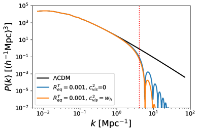
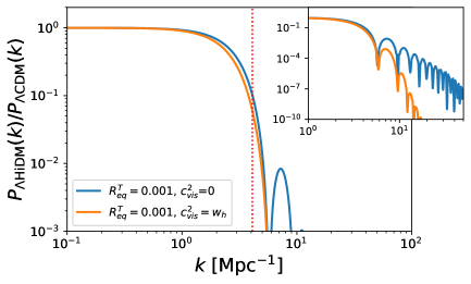
Figure 7: Left: the linear matter power spectrum today in the standard $\Lambda$CDM case and the hidden dark matter case with or without viscosity. The early-time relativistic phase significantly suppresses the power spectrum for small-scale modes with wavenumber larger than $k_{\rm{sup}}$, indicated by the red dashed line (estimated from Eq. (5.2)). A viscosity makes the suppression even more profound. Right: the ratio of the matter power spectra between the $\Lambda$HiDM case and the standard $\Lambda$CDM case, with an inset plot showing a wider range of the y-axis.

The suppression effect is more significant for smaller scales (larger $k$). The larger the $R^{\rm{T}}_{\rm{eq}}$, the smaller the $k_{\rm{sup}}$ and the larger the scale where such a suppression begins to appear. In Figure 7 we show the matter power spectrum with $R^{\rm{T}}_{\rm{eq}}=0$ (standard cold dark matter) and $R^{\rm{T}}_{\rm{eq}}=0.001$. Eq. (5.2) estimates that a suppression should appear when $k\gtrsim 4.1\,[{\rm{Mpc}}^{-1}]$, which is consistent with what is shown in Figure 7.

It is worth pointing out that the suppression of the small-scale matter power spectrum is different from what was found in Ref. [75]. As shown in their Figure 3, the amplitude of the matter power spectrum can be suppressed or enhanced. We investigate such a discrepancy by artificially varying the transition index of the equation of state. We found that an enhancement of the matter power spectrum at small scales only appears for a sharp enough relativistic-to-nonrelativistic transition (i.e., $n_{w}>5$). However, with the evolution derived from first principles based on some realistic assumptions of the dark matter particle nature, the relativistic-to-nonrelativistic transition of our model is rather smooth (with $n_{w}\sim 2$).

From the above discussions, the key to constraining $R^{\rm{T}}_{\rm{eq}}$ is to probe the matter power spectrum at small scales. So far, the large-scale cosmological observation that can probe the smallest scales in the power spectrum is the flux power spectrum of the Lyman-$\alpha$ forest [92, 93, 94]. To be able to provide a consistent explanation for CMB and Lyman-$\alpha$ forest observations, the suppression scale $k_{\rm{sup}}$ must be larger than the scale already probed by the Lyman-$\alpha$ forest. Modeling observations at such small scales requires treatment of non-linear structure formation [36]. While our analysis mainly focuses on the linear regime, we perform an estimation of the upper bound on $R_{\rm{eq}}^{\rm{T}}$ from current Lyman-$\alpha$ forest data. We conservatively take that the matter power spectrum as probed by the Lyman-$\alpha$ forest is overall consistent with the prediction of the standard $\Lambda$CDM model to a scale of $k\sim 0.03$ (km/s)^-1 [94], or $k\sim 3\,h\,{\rm{Mpc}}^{-1}$. According to Eq. (5.2), setting $k_{\rm{sup}}\gtrsim 3\,h\,{\rm{Mpc}}^{-1}$ gives $R^{\rm{T}}_{\rm{eq}}\lesssim 0.0022$ with $h=0.7$. Thus, the Lyman-$\alpha$ forest should be able to provide a stronger constraint on $R_{\rm{eq}}^{\rm{T}}$ than CMB. However, we will show in the latter sections that properties of small-scale galaxies may provide even an order-of-magnitude stronger constraint.

6 Small and minimum scales, halo mass function

So far, we have mainly focused on the phenomenology and constraints of hidden dark matter on linear scales. In this section, we will investigate the effects on the nonlinear scales. These effects should be more rigorously studied by cosmological simulations, but in this work, we will adopt a semi-analytical approach and study the impacts on the halo mass function and the smallest halo mass.

6.1 The halo mass function

As discussed in the previous section, the linear power spectrum is suppressed at scales smaller than the sound horizon, and even further suppressed at scales smaller than the viscous scale when viscosity is present. This can affect the small-scale structures and have a significant impact on the halo mass function. Since we have estimated the suppressed scale in the linear matter power spectrum, we can infer the suppressed mass scale in the halo mass function by the following,

$$M_{\rm{sup}}\simeq\frac{4\pi}{3}\left(\frac{\pi}{k_{\rm{sup}}}\right)^{3}\rho_{\rm{m}}^{0}=1.6\times 10^{11}\,h^{2}\,M_{\odot}\Big{(}\frac{R_{\rm{eq}}^{\rm{T}}}{0.001}\Big{)}^{2.5}\,.$$ (6.1)

This $M_{\rm{sup}}$ is independent of redshift because it corresponds to a comoving scale at which the initial linear power spectrum becomes suppressed. The halo mass function is expected to be significantly reduced for $M<M_{\rm{sup}}$. To show such an effect more explicitly, we calculate the halo mass function by applying the extended Press-Schechter formalism [95, 96, 97, 98] with the Sheth-Tormen fitting equation [99],

$$\frac{dn}{dM}(M,z)=A\sqrt{\frac{2a}{\pi}}\frac{\rho_{\rm{m}}(z)}{M}\frac{-d\ln\sigma(M)}{dM}\nu_{\rm{c}}(z)\Big{[}1+\frac{1}{\big{(}a\nu^{2}_{\rm{c}}(z)\big{)}^{q}}\Big{]}\exp\big{(}-a\nu^{2}_{\rm{c}}(z)/2\big{)}\,,$$ (6.2)

where $M$ is the halo mass and $\rho_{\rm{m}}(z)$ the average matter density at redshift $z$. The function $\sigma(M)$ is the current variance of the linear matter fluctuation averaged over a scale of $M$ and $\nu_{\rm{c}}(z)=\frac{1.686}{D(z)\sigma(M)}$ with $D(z)$ the growth factor normalized to unity today. The fitting constants are $A=0.322$, $a=0.707$ and $q=0.3$. The variance $\sigma(M)$ is calculated by

$$\sigma^{2}(M)=\frac{1}{2\pi^{2}}\int_{0}^{\infty}P_{m}(k)|f_{\rm sh}(kR)|^{2}k^{2}dk\,,$$ (6.3)

where the spherical top-hat function $f_{\rm{sh}}(x)$ is,

$$f_{\rm sh}(x)=\frac{3}{x^{3}}(\sin x-x\cos x)\,,$$ (6.4)

and $R=\left(\frac{3M}{4\pi\rho_{\rm{m}}^{0}}\right)^{1/3}$. To avoid correlated modes in the calculation of $\sigma^{2}(M)$, it is standard to use $f(x)$ as sharp-$k$ window function [99]. However, this only leads to a small difference in practice, so we may neglect this in favor of a spherical top-hat function [Eq. (6.4)] for ease of computation. The above formalism allows us to infer the number of collapsed structures at late times from the linear matter power spectrum, which obtains from our modified camb. We show the resultant halo mass function in Figure 8, where the suppressed mass scale in the halo function estimated by Eq. (6.1) is included. For $R_{\rm{eq}}^{\rm{T}}=0.001$, the number of halos with mass below $M_{\rm{sup}}\simeq 7.8\times 10^{10}M_{\odot}$ (with $h=0.7$) is strongly suppressed independent of redshift. This impact is more pronounced at higher redshifts because fewer halos with $M>M_{\rm{sup}}$ exist: in the standard $\Lambda$CDM model, larger halos are likely to form later. If most of the halos with mass above $M_{\rm{sup}}$ are formed after redshift $z_{1}$ in the standard $\Lambda$CDM model, the entire halo population is expected to be significantly suppressed before $z_{1}$ in the hidden dark matter model. This is shown by the green curves in Figure 8.

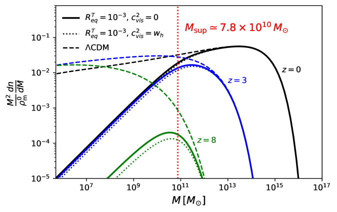
Figure 8: The halo mass function calculated from the extended Press-Schechter formalism. There is a suppressed mass scale $M_{\rm{sup}}$ below which the number of halos is suppressed compared to the $\Lambda$CDM case at all times. For $R^{T}_{eq}=0.001$, this suppression mass scale is $\sim 10^{11}\,M_{\odot}$. Setting the viscosity further suppresses the halo mass function, but the effect is not qualitatively different from the cases without viscosity. The vertical red dotted line indicates the estimated suppression mass scale $M_{\rm{sup}}$ calculated from (6.1).

It is worth pointing out that the Press-Schechter formalism assumes that the temperature (and thus the pressure or the velocity dispersion) of dark matter is negligible during the collapse. The mass function of the dark matter halos is reduced for $M>M_{\rm{sup}}$ due to a suppression of the linear matter power spectrum for $k>k_{\rm{sup}}$, which is the initial condition for the late-time nonlinear collapse. In our scenario, the hidden dark matter has some residual temperature, which leads to another effect that suppresses small-halo formation due to the change of dynamics during the collapse. The situation is analogous to baryon collapse without dark matter at a finite temperature, where in the extreme case there exists some minimum mass scale (the Jeans mass) below which the self gravity of a baryon clump would not be able to overcome the pressure and would not collapse. Due to the residual temperature, there is also a dark-matter “Jeans mass” ($M_{\rm{J}}$) In Appendix E we estimate the Jeans mass at different redshifts. We find it is generally orders of magnitude smaller than $M_{\rm{sup}}$, especially for $z<10$, so we can neglect it for this purpose. This is in agreement with the treatment in Ref. [70] for warm dark matter.

6.2 Constraints from the smallest dark matter halo

Recently there have been significant developments in theoretical and observational studies of low-mass galaxies, which are promising targets to test the nature of dark matter [10, 27, 100, 101, 70, 102, 103, 104]. Here we follow Ref. [27] and use the reported minimum halo mass to perform an order-of-magnitude estimate of the bound on $R_{\rm{eq}}^{\rm{T}}$. By fitting zoom-in simulations to the luminosity distribution of the Milky Way satellites, Ref. [105] reported that the minimum halo mass hosting Milky Way satellites is $<5.4\times 10^{8}M_{\odot}$ at $2\sigma$; also see [106]. In Sec. 6.1 we showed that the population of dark matter halo below some $M_{\rm{sup}}$ [Eq. (6.1)] would be significantly reduced in our hidden matter scenario. We assume that halos with mass below $M_{\rm{sup}}$ are rare enough to be unlikely to be observed and that such a suppression effect is preserved during halo mergers, making subhalos with mass below $M_{\rm{sup}}$ also rare. Then, setting $M_{\rm{sup}}\lesssim 5.4\times 10^{8}M_{\odot}$ gives $R_{\rm{eq}}^{\rm{T}}\lesssim 1.4\times 10^{-4}$.

As an additional check, we can apply this constraint to the case of WDM. Since thermal WDM is a special case in the class of HiDM we studied, the constraint on $R_{\rm{eq}}^{\rm{T}}$ can be translated into a lower bound on the WDM mass of $\sim 2$ keV. This estimate is consistent (within a factor of 2) with the constraints on the WDM mass in [107, 108, 104, 105] where observations at similar scales are considered.

In addition to using the minimum halo mass, Ref. [27] also considered the whole small-galaxy population, which is a more rigorous treatment, and showed that using the minimum halo mass produces a more conservative constraint. Therefore, we expect the actual upper bound on $R_{\rm{eq}}^{\rm{T}}$ from the small-galaxy population to be stronger. But the estimate here is already our strongest constraint on $R_{\rm{eq}}^{\rm{T}}$. Indeed, it is about an order of magnitude stronger than the constraint from the Lyman-$\alpha$ forest, suggesting that the hidden dark matter scenario is phenomenologically indistinguishable from cold dark matter in large-scale cosmology based on current observations.

7 A List of constraints considered in this work

We have individually investigated four different constraints on the hidden dark matter model, as parameterized by $R_{\rm{eq}}^{\rm{T}}$. Different constraints have different constraining powers and physical bases. In Table 3, we summarize all the constraints on $R^{\rm{T}}_{\rm{eq}}$ considered in this work. So far, at cosmological scales, the strongest constraint is from the Lyman-$\alpha$ forest. But at small scales, the subhalo population can provide even a stronger constraint. Thus our work again suggests that the most promising region to study warm-dark-matter-like dark matter models is at small (galactic and subgalactic) scales.

As mentioned in Sec. 2.3, the upper bound on $R_{\rm{eq}}^{\rm{T}}$ can be translated into a lower bound on the particle mass which becomes stronger when $\Delta_{\rm ini}$. For $\Delta_{\rm ini}=0$, the corresponding lower bound is $\sim 2$ keV taking $g$ of order unity. To avoid this mass lower bound, one needs to consider condensation for the boson case or a positive initial chemical potential for the fermion case, or to consider more species (especially, dark radiation) in the dark sector that HiDM interacts with.

Observations	Bounds on $R^{\rm{T}}_{\rm{eq}}$	Bounds on $\hat{z}$	Phenomenological effects
BBN	$\lesssim 0.2$	$>1.7\times 10^{4}$	Modifying the cosmic expansion during the BBN epoch.
Planck 18	$<0.024$ ($2\sigma$)	$>1.4\times 10^{5}$	Adding an effective CDI model at the largest scales.
Lyman-$\alpha$	$\lesssim 2.2\times 10^{-3}$	$>1.5\times 10^{6}$	Suppressing the small-scale matter power spectrum.
Small halos	$\lesssim 1.4\times 10^{-4}$	$>1.8\times 10^{7}$	Reducing population of halos with mass below $M_{\rm{sup}}$.

Table 3: Summary of the constraints on $R^{\rm{T}}_{\rm{eq}}$ considered in this work. The constraints on $R_{\rm{eq}}^{\rm{T}}$ are also translated into the constraints on the redshift at the transition ($\hat{z}=1/\hat{a}-1$). Only the constraint from Planck is obtained from a likelihood analysis, while others are estimated. We use “$\lesssim$” for estimated constraints. Constraints in the last three rows correspond to the cases without viscosity. Setting on the viscosity would lead to slightly tighter constraints, so they can be viewed as conservative constraints.

7.1 Remarks on other cosmological/astrophysical phenomenology

We have shown that for the background evolution and large-scale structure formation, the most important property in our HiDM scenario is the time of the relativistic-to-nonrelativistic transition, parameterized by $R_{\rm{eq}}^{\rm{T}}$. There are phenomenological similarities between our HiDM and the WDM scenario. Properties other than $R_{\rm{eq}}^{\rm{T}}$ only make small differences in the impacts on cosmological observables.

If confirmed, the global 21cm absorption signal [109] may provide another cosmological constraint on $R_{\rm{eq}}^{\rm{T}}$. The idea is similar to that in Refs. [37, 38, 110]: the suppression of the small-scale matter power spectrum would significantly delay formation of small-mass halos (see also Sec. 6.1), which would postpone the star formation that produces Lyman-$\alpha$ photons. The coupling between the spin temperature and the gas temperature, mediated by the Lyman-$\alpha$ background, could be too late if the suppression is too large, putting a constraint on $R_{\rm{eq}}^{\rm{T}}$. However, the astrophysical uncertainties are large, e.g., the early-time star formation rate and the fraction of the Lyman-$\alpha$ photons that escape halos. Given these uncertainties, a 21cm constraint requires astrophysical modeling beyond the scope of this work.

Other astrophysical observations may help resolve the other intrinsic properties of the Hidden DM. For instance, the difference in particle mass can impact halo formation and some other astrophysical phenomena, such as halo core profiles [111, 112, 113, 112, 114, 115, 116, 117] and annihilation or decay products [11, 12, 13, 14, 15, 16, 17, 18, 19, 20]. Ref [111] showed that by considering the halo profile and minimum halo mass, an upper bound on the mass of single-species fermionic dark matter ($\gtrsim 2$ keV) can be obtained regardless of the cosmological thermal initial condition (e.g., the initial chemical potential). The strength of self-interaction that determines whether HiDM is in equilibrium or free streaming has been shown to also have an impact on the halo profile; see [107, 108, 27, 118, 119, 120] and references therein. The star formation rate at high redshift has also been shown to depend on the dark matter mass in the usual WDM scenario [121].

8 Summary and conclusion

We have studied the cosmological phenomenology of a hidden dark matter model with its own thermal evolution in the context of conserved comoving particle number and comoving entropy. We investigate the impact of cases with different quantum statistics and an initial chemical potential that controls particle occupation number, and in which the dark matter is either in its own thermal equilibrium or free streaming. We found that different cases exhibit similar background evolution as long as the initial chemical potential is nonpositive, which can be well approximated by a set of functions with only one additional parameter (compared to the $\Lambda$CDM case): the characteristic scale factor $\hat{a}$ that determines the time of the relativistic-to-nonrelativistic transition. For a given $\hat{a}$, cosmological phenomenology is insensitive to the particle mass, initial temperature, and intrinsic degrees of freedom, and only weakly depends on the initial chemical potential, whether the dark matter is a fermion or boson, and whether it is in equilibrium or free streaming.

On the perturbation level, we treat the equilibrium case and free-streaming case differently by turning off or on a viscosity parameter. But here again, we find that both cases have similar effects on cosmological observations. For large scales relevant to observations of the CMB temperature and polarization, the effects of hidden dark matter are equivalent to an additional correlated CDI perturbation mode with a specific isocurvature spectrum index. For smaller scales, the matter power spectrum is significantly suppressed, which is a typical feature when the dark matter has some velocity dispersion or pressure to stabilize against linear growth and nonlinear gravitational collapse. At nonlinear scales, we studied phenomenology by calculating the halo mass function using the extended Press-Schechter formalism. Due to the suppression of the matter power spectrum at small scales, the number of small halos at all redshifts is significantly reduced below a mass scale $M_{\rm{sup}}$ that depends on the transition scale factor.

Finally, we estimated the constraints on the transition scale factor individually from BBN, Planck 2018 baseline data, the Lyman-$\alpha$ forest, and the smallest observed subhalo mass. These observations constrain the transition time in different ways, with the strongest constraint arising from the population of subhalos. Based on the reported minimum subhalo mass, we conservatively estimate the transition redshift to be higher than $1.8\times 10^{7}$, which is about an order of magnitude stronger than the Lyman-$\alpha$-forest constraint. This means that the most promising regime to constrain or detect effects from the hidden dark matter model is likely to be at the smallest galaxy systems. A promising future avenue is to explore how such a suppression of the small-halo population could affect cosmic reionization and the current subhalo population, although further efforts in disentangling other baryon effects are needed for robust studies.

Along with a number of recent works in the literature, our work shows that structure formation at galaxies scales is promising for the study of warm-dark-matter-like models. Looking ahead, a number for near-future galaxy surveys from LSST, DESI, Euclid, WFIRST and JWST will deliver a plethora of data to study dwarf galaxies. It will be an exciting era to study dark matter and potentially discover beyond CDM physics.

Appendix A Details of solving for the background evolution - thermal equilibrium case

With the phase space equilibrium distribution given in Eq. (2.1), the particle number density, energy density and pressure are given by,

$$n_{\rm{h}}(x,\Delta) =\frac{gm^{3}}{2\pi^{2}\hbar^{3}}\frac{1}{x^{3}}\mathcal{N}(x,\Delta)\,,~{}~{}\textrm{with~{}~{}~{}}\mathcal{N}(x,\Delta)=\int_{0}^{\infty}\frac{dzz^{2}}{\exp(\sqrt{z^{2}+x^{2}}-x-\Delta)\pm 1}\,;$$ (A.1)

$$\rho_{\rm{h}}(x,\Delta) =\frac{gm^{4}}{2\pi^{2}\hbar^{3}}\frac{1}{x^{4}}\mathcal{R}(x,\Delta)\,,~{}~{}\textrm{with~{}~{}~{}}\mathcal{R}(x,\Delta)=\int_{0}^{\infty}\frac{dzz^{2}\sqrt{z^{2}+x^{2}}}{\exp(\sqrt{z^{2}+x^{2}}-x-\Delta)\pm 1}\,;$$ (A.2)

$$p_{\rm{h}}(x,\Delta) =\frac{gm^{4}}{2\pi^{2}\hbar^{3}}\frac{1}{x^{4}}\mathcal{P}(x,\Delta)\,,~{}~{}\textrm{with~{}~{}~{}}\mathcal{P}(x,\Delta)=\frac{1}{3}\int_{0}^{\infty}\frac{dzz^{4}/\sqrt{z^{2}+x^{2}}}{\exp(\sqrt{z^{2}+x^{2}}-x-\Delta)\pm 1}\,,$$ (A.3)

with +1 for fermions and -1 for bosons. We have used $\Delta$ instead of $y$ in the above equations for reasons that shall be seen. From Euler’s theorem on homogeneous functions, we can obtain the entropy density $s_{\rm{h}}$ as

$$s_{\rm{h}}=\frac{\rho_{\rm{h}}+p_{\rm{h}}-\mu n_{\rm{h}}}{T}\,.$$ (A.4)

Then the specific entropy reads

$$\frac{s_{\rm{h}}}{n_{\rm{h}}}=\frac{\xi(x,\Delta)}{\mathcal{N}(x,\Delta)}-x-\Delta\,,$$ (A.5)

where $\xi(x,\Delta)\equiv\mathcal{R}(x,\Delta)+\mathcal{P}(x,\Delta)$.

It is convenient to use $\Delta$ instead of y for the following reasons. In the relativistic limit $x\rightarrow 0$, we have $\Delta\rightarrow y$ and it is the ratio of the chemical potential and the temperature. The nonrelativistic limit of Eq. (2.1) reads,

$$f(p;x\equiv\frac{m}{T}\rightarrow\infty)=\frac{g}{2\pi^{2}\hbar^{3}}\frac{p^{2}}{\exp\big{[}(\frac{p^{2}}{2m}-\mu+m)/T\big{]}\pm 1}\,.$$ (A.6)

Therefore $\mu-m$ is the effective chemical potential in the nonrelativistic limit, and $\Delta\equiv\frac{\mu-m}{T}$ is the ratio between the effective chemical potential and the temperature. So, the physical meaning of $\Delta$ is more transparent than that of $y$. When $\Delta\ll-1$, the distribution is classical. Quantum statistic effects take place when $\Delta\gtrsim-1$. For fermions, these effects manifest as a degenerate pressure, which is larger for larger $\Delta$. For bosons, the pressure will be smaller for larger $\Delta$. Bose-Einstein condensation begins to take place when $\Delta=0$, which is beyond the scope of this work; we restrict ourselves to the case that $\Delta\leq 0$ for both fermion and boson cases.

It is expected that the hidden dark matter is relativistic ($x\rightarrow 0$) at early times as $a\rightarrow 0$ but later becomes nonrelativistic ($x\rightarrow\infty$). When $x\rightarrow 0$, to leading order we have

$$n_{\rm{h}}(x\rightarrow 0,\Delta\leq 0) =\frac{gm^{3}}{2\pi^{2}\hbar^{3}}\frac{F_{3}^{\mp}(\Delta)}{x^{3}}\,,$$ (A.7)

$$\rho_{\rm{h}}(x\rightarrow 0,\Delta\leq 0) =\frac{gm^{4}}{2\pi^{2}\hbar^{3}}\frac{F_{4}^{\mp}(\Delta)}{x^{4}}\,,$$ (A.8)

$$p_{\rm{h}}(x\rightarrow 0,\Delta\leq 0) =\frac{1}{3}\rho_{\rm{h}}(x\rightarrow 0,\Delta\leq 0)\,,$$ (A.9)

$$\textrm{where~{}~{}~{}~{}~{}}F_{s}^{\mp}(\Delta)\equiv f^{\mp}_{s}(\Delta)\Gamma(s)\exp(\Delta) ~{}~{}~{}~{}~{}~{}{\textrm{and,~{}~{}~{}~{}}}f^{\mp}_{s}(\Delta)\equiv\sum_{n=0}^{\infty}\frac{(\mp 1)^{n}}{(n+1)^{s}}\exp(n\Delta)\,,$$ (A.10)

where now we have $-$ for fermions and $+$ for bosons. $\Gamma(s)$ above is the gamma function. Some special values of $f_{s}^{\mp}$ are $f_{s}^{\mp}(\Delta\ll-1)=1$, $f_{s}^{+}(0)=\zeta(s)$ and $f_{s}^{-}(0)=(1-2^{1-s})\zeta(s)$, where $\zeta(s)$ is the zeta function. A useful property of the function $f_{s}^{\mp}$ is $\frac{d}{d\Delta}\big{(}f_{s}^{\mp}(\Delta)\exp(\Delta)\big{)}=f_{s-1}^{\mp}(\Delta)\exp(\Delta)$ for $s>2$. From the above relativistic limits, the solutions satisfying number conservation [$d(na^{3})=0$] and the first law of thermodynamics with an adiabatic process [$d(\rho_{\rm{h}}a^{3})=-pda^{3}$] are $x\propto a$ and $\Delta=$ constant. From Eq. (A.4), we also have

$$s_{\rm{h}}(x\rightarrow 0,\Delta\leq 0)=n_{\rm{h}}\times\Big{(}\frac{4f^{\mp}_{4}(\Delta)}{f^{\mp}_{3}(\Delta)}-\Delta\Big{)}\,.$$ (A.11)

As $a$ increases, the hidden dark matter will eventually become nonrelativistic. In the nonrelativistic limit ($x\rightarrow\infty$), to the next leading order we have

$$n_{\rm{h}}(x\rightarrow\infty,\Delta\leq 0) =\frac{gm^{3}}{2\pi^{2}\hbar^{3}}\frac{\sqrt{2}}{x^{3/2}}\Big{(}F_{3/2}^{\mp}(\Delta)+\frac{5}{4x}F_{5/2}^{\mp}(\Delta)+\mathcal{O}(\frac{1}{x^{2}})\Big{)}\,,$$ (A.12)

$$\rho_{\rm{h}}(x\rightarrow\infty,\Delta\leq 0) =\frac{gm^{4}}{2\pi^{2}\hbar^{3}}\frac{\sqrt{2}}{x^{3/2}}\Big{(}F_{3/2}^{\mp}(\Delta)+\frac{9}{4x}F_{5/2}^{\mp}(\Delta)+\mathcal{O}(\frac{1}{x^{2}})\Big{)}$$ (A.13)

$$=mn_{\rm{h}}\times\left(1+\frac{3}{2x}\frac{f_{5/2}^{\mp}(\Delta)}{f_{3/2}^{\mp}(\Delta)}+\mathcal{O}(\frac{1}{x^{2}})\right)\,,$$

$$p_{\rm{h}}(x\rightarrow\infty,\Delta\leq 0) =\frac{gm^{4}}{2\pi^{2}\hbar^{3}}\frac{2\sqrt{2}}{3x^{5/2}}\Big{(}F_{5/2}^{\mp}(\Delta)+\mathcal{O}(\frac{1}{x})\Big{)}$$ (A.14)

$$=\frac{mn_{\rm{h}}}{x}\times\left(\frac{f_{5/2}^{\mp}(\Delta)}{f_{3/2}^{\mp}(\Delta)}+\mathcal{O}(\frac{1}{x^{2}})\right)\,,$$

again with $-1$ for fermions and $+1$ for bosons. We need to keep terms up to the next leading order here since the leading order of $\rho_{\rm{h}}$ is trivially the rest energy density and it is the next order that reveals the evolution of the x and $\Delta$. From the above nonrelativisitc limits, the solutions satisfying the number conservation and the first law of thermodynamics are $x\propto a^{2}$ and $\Delta=$ another constant. A much easier way to see why $\Delta$ becomes another constant at the nonrelativistic limit is the following. At the nonrelativistic limit, plugging Eqs. (A.13) and (A.14) into Eq. (A.4) we have

$$s_{\rm{h}}(x\rightarrow\infty,\Delta\leq 0)=n_{\rm{h}}\times\Big{(}\frac{5}{2}\frac{f_{5/2}^{\mp}(\Delta)}{f_{3/2}^{\mp}(\Delta)}-\Delta\Big{)}\,.$$ (A.15)

Since the specific entropy ($s_{\rm{h}}/n_{\rm{h}}$) is a constant, the factor $\big{[}-\Delta+\frac{5}{2}\frac{f_{5/2}^{\mp}(\Delta)}{f_{3/2}^{\mp}(\Delta)}\big{]}$ must be a constant and so is $\Delta$. By equating the relativistic and nonrelativistic limits of $s_{\rm{h}}/n_{\rm{h}}$, we can also derive a consistency relation between the initial $\Delta_{\rm{ini}}$ at the relativistic limit and the final $\Delta_{\rm{f}}$ at the nonrelativistic limit,

$$4\frac{f^{\mp}_{4}(\Delta_{\rm{ini}})}{f^{\mp}_{3}(\Delta_{\rm{ini}})}-\Delta_{\rm{ini}}-\frac{5}{2}\frac{f^{\mp}_{5/2}(\Delta_{\rm{f}})}{f^{\mp}_{3/2}(\Delta_{\rm{f}})}+\Delta_{\rm{f}}=0\,.$$ (A.16)

In particular, from $f_{s}^{\mp}(\Delta\ll-1)=1$ we have in the classical case that $\lim\limits_{\Delta_{\rm{ini}}\rightarrow-\infty}(\Delta_{\rm{f}}-\Delta_{\rm{ini}})=-1.5$. We will use the above consistency relation to check our numerical solutions. We shall see that $\Delta$ never increases. So $\Delta\leq 0$ at all times if it is initially so, which also justifies our restriction that $\Delta\leq 0$.

From the above analyses, we know that $x$ first increases as $a$ and then as $a^{2}$, and $\Delta$ gradually changes from one constant to another. Guided by these, we will now derive and solve the differential equations for $x(a)$ and $\Delta(a)$, and then calculate $n_{\rm{h}}(a)$, $\rho_{\rm{h}}(a)$, $p_{\rm{h}}(a)$ and $s_{\rm{h}}(a)$ using Eqs. (A.1) to (A.4). The evolution equations for $x$ and $\Delta$ are obtained by keeping the total particle number and the specific entropy of the hidden dark matter unchanged, i.e., $d(n_{\rm{h}}a^{3})=0$ and $d(s_{\rm{h}}/n_{\rm{h}})=0$. These give the following infinitesimal evolution of $x$ and $\Delta$ in a matrix form,

$$\begin{pmatrix}d\ln x\\ d\Delta\end{pmatrix}=\bm{M}^{-1}\begin{pmatrix}d\ln a\\ 0\end{pmatrix}\,,$$ (A.17)

with $$\bm{M}\equiv\begin{pmatrix}1-\frac{x}{3\mathcal{N}}\mathcal{N}_{x}&-\frac{1}{3\mathcal{N}}\mathcal{N}_{\Delta}\\ \frac{x}{\mathcal{N}}\xi_{x}-\frac{x\,\xi}{\mathcal{N}^{2}}\mathcal{N}_{x}-x&~{}~{}\frac{1}{\mathcal{N}}\xi_{\Delta}-\frac{\xi}{\mathcal{N}^{2}}\mathcal{N}_{\Delta}-1\end{pmatrix}\,,$$ (A.18)

where a subscript denotes differentiation (e.g., $\xi_{x}\equiv\frac{\partial\xi}{\partial x}$) and

$$\mathcal{N}_{x} =\int_{0}^{\infty}dz\frac{z^{2}\exp(\sqrt{z^{2}+x^{2}}-x-\Delta)}{\big{[}\exp(\sqrt{z^{2}+x^{2}}-x-\Delta)\pm 1\big{]}^{2}}\Big{(}1-\frac{x}{\sqrt{z^{2}+x^{2}}}\Big{)}\,,$$ (A.19)

$$\mathcal{N}_{\Delta} =\int_{0}^{\infty}dz\frac{z^{2}\exp(\sqrt{z^{2}+x^{2}}-x-\Delta)}{\big{[}\exp(\sqrt{z^{2}+x^{2}}-x-\Delta)\pm 1\big{]}^{2}}\,,$$ (A.20)

$$\xi_{x} =\int_{0}^{\infty}dz\frac{z^{2}}{\exp(\sqrt{z^{2}+x^{2}}-x-\Delta)\pm 1}\Bigg{[}\frac{(\sqrt{z^{2}+x^{2}}-x)(1+\frac{z^{2}}{3(z^{3}+x^{2})})}{1\pm\exp(-\sqrt{z^{2}+x^{2}}+x+\Delta)}+\frac{x}{\sqrt{z^{2}+x^{2}}}-\frac{xz^{2}}{3(z^{2}+x^{2})}\Bigg{]}\,,$$ (A.21)

$$\xi_{\Delta} =\int_{0}^{\infty}dz\frac{z^{2}\exp(\sqrt{z^{2}+x^{2}}-x-\Delta)}{\big{[}\exp(\sqrt{z^{2}+x^{2}}-x-\Delta)\pm 1\big{]}^{2}}\Big{[}\sqrt{z^{2}+x^{2}}+\frac{z^{2}}{3\sqrt{z^{2}+x^{2}}}\Big{]}\,.$$ (A.22)

Given the initial conditions of $x$ and $\Delta$, the above equations are solved by integrating from a very small $a$ when $x\ll 1$ to $a=1$. We can also write Eq. (A.17) in the form of decoupled differential equations

$$\frac{d\bm{y}}{d\ln a}=\bm{f}\,,$$ (A.23)

where $\bm{y}=(\ln x,\,\Delta)$ and $f_{i}=(\bm{M}^{-1})_{i1}$.

By solving the evolution of $x$ and $\Delta$, we can also obtain the (squared) adiabatic sound speed squared $c_{\rm{s}}^{2}$ that is used at the perturbation level. This can be done by restricting $\delta x$ and $\delta\Delta$ to the path (in the state variable space) that keeps the specific entropy unchanged. For matter that has only two independent state variables (e.g., $T$ and $\mu$ here), this perturbation path is unique and is $(\delta x,\delta\Delta)\propto\big{(}M_{22},-M_{12}\big{)}$. But since we also assume the background evolution is keeping the specific entropy unchanged, all state variables’ infinitesimal time variations must be along the same path. All perturbed quantities ($\delta x$, $\delta\Delta$, $\delta\rho_{\rm{h}}$, $\delta p_{\rm{h}}$) must then be proportional to their infinitesimal temporal variations ($dx$, $d\Delta$, $d\rho_{\rm{h}}$, $dp_{\rm{h}}$). Therefore, there are two methods of obtaining the adiabatic sound speed, which are

$$\begin{split}\frac{\delta p_{\rm{h}}}{\delta\rho_{\rm{h}}}&=\frac{\frac{\partial p_{\rm{h}}}{\partial x}\delta x+\frac{\partial p_{\rm{h}}}{\partial\Delta}\delta\Delta}{\frac{\partial\rho_{\rm{h}}}{\partial x}\delta x+\frac{\partial\rho_{\rm{h}}}{\partial\Delta}\delta\Delta}\\ &=\frac{(4-x\mathcal{P}_{x})M_{22}+\mathcal{P}_{\Delta}M_{12}}{(4-x\mathcal{R}_{x})M_{22}+\mathcal{R}_{\Delta}M_{12}}\,,\textrm{~{}~{}~{}(method 1)}\\ &=\frac{dp_{\rm{h}}}{d\rho_{\rm{h}}}\rm{~{}~{}or~{}~{}}\frac{dp_{\rm{h}}/da}{d\rho_{\rm{h}}/da}\,.\textrm{~{}~{}~{}~{}(method 2)}\end{split}$$ (A.24)

Method 1 is valid if the perturbations are isentropic, while method 2 is valid if the perturbations and the background evolutions are both isentropic. We have verified the equivalence of the above two methods when both the background evolution and the perturbations are isentropic. The evolution of the adiabatic sound speed is also shown in the lower middle panel of Figure 1. We can see that $\delta p_{\rm{h}}/\delta\rho_{\rm{h}}$ has a very similar scale-factor dependence as $w_{\rm{h}}$ but with a delayed transition time.

Appendix B Details of finding a parameterized background evolution

B.1 A parameterized background evolution

The hidden dark matter began relativistic, with a temperature $T_{\rm{h}}$ different from that of the Standard Model particles. After $T_{\rm{h}}$ dropped below the mass of the hidden baryon ($m_{\rm{h}}$), it transitioned to the nonrelativistic case. We find that the evolution of the equation-of-state parameter $w_{\rm{h}}(a)$ can be well approximated by the following parameterized function,

$$w_{\rm{h}}(a)=\frac{1}{3}\frac{a_{\rm{T}}^{n}}{a^{n}+a_{\rm{T}}^{n}}\,,$$ (B.1)

where $a_{\rm{T}}$ specifies the transition scale factor and the positive transition index $n$ determines the transition width. The equation-of-state parameter approaches $1/3$ for $a\ll a_{\rm{T}}$ and $0$ for $a\gg a_{\rm{T}}$. The transition is shallower (sharper) for a smaller (larger) $n$. Note that we do not restrict $n$ to be an integer. With the above parameterized $w_{\rm{h}}$, the energy density can be calculated analytically and reads,

$$\rho_{\rm{h}}(a)=\frac{\rho_{\rm{h}}^{0}}{a^{4}}\left(\frac{a^{n}+a_{\rm{T}}^{n}}{1+a_{\rm{T}}^{n}}\right)^{\frac{1}{n}}\,,$$ (B.2)

where the superscript or subscript “0” denotes today and we normalize the scale factor today to unity $a_{0}=1$. We require that dark matter is highly nonrelativistic today, $a_{\rm{T}}\ll 1$. For $n$ of the order of unity, we have $\rho_{\rm{h}}\simeq\rho_{\rm{h}}^{0}/a^{3}$ at late times when $a\gg a_{\rm{T}}$ and $\rho_{\rm{h}}\simeq\rho_{\rm{h}}^{0}a_{\rm{T}}/a^{4}$ at early times when $a\ll a_{\rm{T}}$. Examples of the parameterized equation of state parameter are shown in Figure 9.

Figure 9: Examples of a relatively smooth (n=1) and a relatively sharp (n=10) transition described by a parameterized equation-of-state parameter $w_{\rm{h}}(a)$ given by in Eq. (B.1).

At the perturbation level, we will also need the squared sound speed $c_{\rm{s}}^{2}\equiv\delta p_{\rm{h}}/\delta\rho_{\rm{h}}$. If we assume that the specific entropy is unchanged for both the background evolution and perturbations of the hidden dark matter, the sound speed can be calculated as

$$\begin{split}\frac{\delta p_{\rm{h}}}{\delta\rho_{\rm{h}}}&=\frac{dp_{\rm{h}}/da}{d\rho_{\rm{h}}/da}\,,\textrm{~{}~{}~{}~{}~{}~{}~{}~{}~{}if both background and perturbations are isentropic,}\\ &=\frac{1}{3}\frac{\tfrac{4}{3}a_{\rm{T}}^{n}}{a^{n}+\tfrac{4}{3}a_{\rm{T}}^{n}}\,,\textrm{~{}~{}~{}~{}~{}using the parameterized }w_{\rm{h}}(a)\textrm{ from Eq.\,\eqref{eq:HiDM-w-parameterization}.}\end{split}$$ (B.3)

Note that $\delta p_{\rm{h}}/\delta\rho_{\rm{h}}$ has the same functional dependence on $a$ as $w_{\rm{h}}(a)$ with the same transition index but a larger transition scale factor $a_{\rm{T}}^{\prime}=(\frac{4}{3})^{\tfrac{1}{n}}\times a_{\rm{T}}$. On a logarithmic scale, the transition “gap” is $\log_{10}a_{\rm{T}}^{\prime}-\log_{10}a_{\rm{T}}=\frac{1}{n_{w}}\log_{10}(4/3)$.

We will fit Eq. (B.2) into the numerical result of $\rho_{h}$ to determine the best-fit transition index $n_{w}$ and transition scale $a_{\rm{T}}^{w}$. These $n_{w}$ and $a_{\rm{T}}^{w}$ will be used in Eq. (B.1) to approximate the evolution of $w_{\rm{h}}$. For $c_{\rm{s}}^{2}$, since Eq. (B.3) has the same form as Eq. (B.1), instead of using Eq. (B.3) we use another Eq. (B.1) with a different set of $n_{c_{\rm{s}}^{2}}$ and $a_{\rm{T}}^{c_{\rm{s}}^{2}}$ to fit $c_{\rm{s}}^{2}(a)$ for a better approximation to the numerical result. According to the above discussions, we should have $n_{c_{\rm{s}}^{2}}\simeq n_{w}$ and $a_{\rm{T}}^{c_{\rm{s}}^{2}}\simeq(\frac{4}{3})^{1/n_{w}}\times a_{\rm{T}}^{w}$; we will use these conditions to check our results.

B.2 Parameterized approximation I: the thermal equilibrium case

Let us see what can affect the background evolution. In the classical limit ($\Delta\ll-1$), the transition profile is independent of $\Delta_{\rm{ini}}$. All other parameters associated with the particle nature, e.g. $g$ and $m$, can be absorbed into another single parameter: the hidden dark matter energy density fraction today $\Omega_{\rm{h}}$. Therefore, when $\Delta_{\rm{ini}}\ll-1$ the evolution of energy density and equation of state of the hidden dark matter is determined by only two parameters: $\Omega_{\rm{h}}$ and $\hat{a}$. When $\Delta_{\rm{ini}}\gtrsim-1$, quantum statistics plays a role in the evolution. Let us take the equation of state parameter $w_{\rm{h}}$ as an example. It does not depend on $\Omega_{\rm{h}}$ and generally we can write it as a function of $a$ that depends on $\hat{a}$, $\Delta_{\rm{ini}}$, and the underlying statistics,

$$w_{\rm{h}}=w_{\rm{h}}(a;\hat{a},\Delta_{\rm{ini}},\pm)\,,$$ (B.4)

where “$+$” here stands for Fermi-Dirac statistics and “$-$” for Bose-Einstein statistics. We define the classical limit of $w_{\rm{h}}$ as

$$w_{\rm{h}}^{\rm{class.}}(a;\hat{a})\equiv w_{\rm{h}}(a;\hat{a},\Delta_{\rm{ini}}\ll-1,\pm)\,.$$ (B.5)

We shall show in Sec. C that its dependence on $\Delta_{\rm{ini}}$ or the underlying statistics is rather weak. Similarly, the evolution of other variables can be written as $x=x(a;\hat{a},\Delta_{\rm{ini}},\pm)$, $\rho_{\rm{h}}=\rho_{\rm{h}}(a;\Omega_{\rm{h}},\hat{a},\Delta_{\rm{ini}},\pm)$, $p_{\rm{h}}=p_{\rm{h}}(a;\Omega_{\rm{h}},\hat{a},\Delta_{\rm{ini}},\pm)$ and $\delta p_{\rm{h}}/\delta\rho_{\rm{h}}=c_{\rm{s}}^{2}(a;\hat{a},\Delta_{\rm{ini}},\pm)$, etc. They all have classical limits that only depend on $\hat{a}$, or in addition, on $\Omega_{\rm{h}}$; see Sec. C.

The background evolution can be very well approximated by the parameterization presented in Sec. B.1. To do this, we look for the $\rho_{\rm{h}}^{\rm{approx}}$ [parameterized by $n$ and $a_{\rm{T}}$ in Eq. (B.2)] that best matches the numerical solution of $\rho_{\rm{h}}$. Note that we choose to match $\rho_{\rm{h}}$ instead of $w_{\rm{h}}$ because the energy density is more physically important than the equation of state parameter. Our best-fit $\rho_{\rm{h}}^{\rm{approx}}$ is defined to be one that minimizes the following difference:

$${\rm{Difference}}=\int d\ln(a)\big{[}\ln\rho_{\rm{h,N}}(a;\hat{a},\Delta_{\rm{ini}},\pm)-\ln\rho_{\rm{h,N}}^{\rm{approx}}(a;n_{w},\delta_{w}^{a})\big{]}^{2}\,,$$ (B.6)

where $\delta_{w}^{a}\equiv\log_{10}a_{\rm{T}}^{w}-\log_{10}{\hat{a}}$ is the offset of $a_{\rm{T}}^{w}$ related to $\hat{a}$ in a logarithmic scale, and the normalized energy densities are defined as $\rho_{\rm{h,N}}\equiv\frac{\rho_{\rm{h}}}{gm^{4}/(2\pi^{2}\hbar^{3})}$ and $\rho_{\rm{h,N}}^{\rm{approx}}\equiv\frac{\rho_{\rm{h}}^{\rm{approx}}}{gm^{4}/(2\pi^{2}\hbar^{3})}$ (so that the $\Omega_{\rm{h}}$ dependence is canceled out). The superscript/subscript $w$ denotes the fitting parameters for $\rho_{\rm{h}}$ and $w_{\rm{h}}$, which are to be distinguished from the parameters for the sound speed later. Using Eq. (B.2) and imposing $\rho_{\rm{h}}^{\rm{approx}}(a\rightarrow 0)=\rho_{\rm{h}}(a\rightarrow 0)$, we obtain the normalized density fitting function as

$$\rho_{\rm{h,N}}^{\rm{approx}}(a)=\big{(}\lim\limits_{a\rightarrow 0}\frac{a}{x}\big{)}^{4}\frac{F_{4}^{\mp}(\Delta_{\rm{ini}})}{a^{4}}\big{[}1+(a/a_{\rm{T}}^{w})^{n_{w}}\big{]}^{\frac{1}{n_{w}}}\,.$$ (B.7)

We vary $n_{w}$ and $a_{\rm{T}}^{w}$ (or equivalently $\delta_{w}^{a}$) to minimize Eq. (B.6). Once the best-fit $n_{w}$ and $a_{\rm{T}}^{w}$ are found, we calculate $w_{\rm{h}}^{\rm{approx}}$ with Eq. (B.1) to approximate the numerical evolution of $w_{\rm{h}}$. We show in the left panel of Figure 3 the fractional difference between an example of the numerical evolution of the energy density and its best-fit approximation. In this example, we take a fermionic hidden dark matter with $\Delta_{\rm{ini}}=0$ and $\lim\limits_{x\rightarrow 0}\frac{x}{a}=10^{4}$. The difference between the numerical solution and the approximation is within $0.5\%$ at all times. In the middle panel, we show the numerical solution of $w_{\rm{h}}$ (solid black) of the same example and its approximation $w_{\rm{h}}^{\rm{approx}}$ [dashed red, calculated with Eq. (B.1)]. They also match very well. Table 2 lists the best-fit parameters for some special cases. We find that the transition index is about $n_{w}\simeq 1.8$ for all cases of interest, which means the transition is rather smooth. We also find $\delta_{w}^{a}$ is from $-0.095$ to $-0.085$, so $a_{\rm{T}}^{w}$ is slightly smaller than $\hat{a}$.

The next step is to determine the evolution of the adiabatic sound speed $c_{\rm{s}}^{2}$. We could use Eq. (B.3) to calculate it with the same $n_{w}$ and $a_{\rm{T}}^{w}$. However, we pointed out earlier that Eq. (B.3) has the same functional dependence on $a$ as Eq. (B.1). For a closer approximation to the numerical solution, it is better to fit the evolution of the sound speed using another fitting function $c_{\rm{s,approx}}^{2}$ of the form of Eq. (B.1) but with another set of $n_{c_{\rm{s}}^{2}}$ and $\delta_{c_{\rm{s}}^{2}}^{a}$. That is, we look for the approximation $c_{\rm{s,approx}}^{2}$ that minimizes the following difference,

$${\rm{Difference}^{\prime}} =\int d\ln(a)\big{[}c_{\rm{s}}^{2}(a;\hat{a},\Delta_{\rm{ini}},\pm)-c_{\rm{s,approx}}^{2}(a;n_{c_{\rm{s}}^{2}},\delta_{c_{\rm{s}}^{2}}^{a})\big{]}^{2}\,,$$ (B.8)

$${\rm{with}} ~{}~{}~{}~{}~{}c_{\rm{s,approx}}^{2}=\frac{1}{3}\frac{1}{(a/a_{\rm{T}}^{c_{\rm{s}}^{2}})^{n_{c_{\rm{s}}^{2}}}+1}\,,$$ (B.9)

where $\delta_{c_{\rm{s}}^{2}}^{a}\equiv\log_{10}a_{\rm{T}}^{c_{\rm{s}}^{2}}-\log_{10}{\hat{a}}$ is the offset of $a_{\rm{T}}^{c_{\rm{s}}^{2}}$ relative to $\hat{a}$ on a logarithmic scale. The superscript/subscript $c_{\rm{s}}^{2}$ denotes the fitting parameters for the sound speed, which are different from those for $\rho_{\rm{h}}$ and $w_{\rm{h}}$. The best-fit parameters for the sound speed are also listed in Table 2. We find that the best-fit transition index is about $n_{c_{\rm{s}}^{2}}=1.9$ for all cases. So, the sound speed transition is slightly sharper than the equation of state transition. The offset $\delta_{c_{\rm{s}}^{2}}^{a}$ is from $0.032$ to $0.044$, slightly larger than $\delta_{w}^{a}$, which means the transition of the sound speed is slightly delayed compared to the equation of state parameter. But the transition “gap” $\delta_{c_{\rm{s}}^{2}}^{a}-\delta_{w}^{a}$ is different from, and almost twice as large as the $\frac{1}{n_{w}}\log_{10}(4/3)$ that would be expected if we used Eq. (B.3) to calculate the adiabatic sound speed. Therefore, for a better approximation to the numerical solutions, we will use one set of $\delta_{a}^{w}$ and $n_{w}$ for the approximation of $\rho_{\rm{h}}$ and $w_{h}$ and another set of $\delta_{a}^{c_{\rm{s}}^{2}}$ and $n_{c_{\rm{s}}^{2}}$ for $c_{\rm{s}}^{2}$.

We can also determine the values of $\hat{a}$ and $C$ according to their definitions in Eqs. (2.7) and (2.8). The constant $C$ can be determined from the conservation of comoving number density and the fact that $C=\big{(}\lim\limits_{x\rightarrow 0}\frac{x}{a}\big{)}^{2}\big{/}\big{(}\lim\limits_{x\rightarrow\infty}\frac{x}{a^{2}}\big{)}$. From Eqs. (A.7) and (A.12) we have

$$C=\frac{2}{\pi^{1/3}}\Big{[}\frac{f_{3}^{\mp}(\Delta_{\rm{ini}})}{f_{3/2}^{\mp}(\Delta_{\rm{f}})}\Big{]}^{\frac{2}{3}}\exp\big{(}\frac{2}{3}(\Delta_{\rm{ini}}-\Delta_{\rm{f}})\big{)}\,,$$ (B.10)

where $\Delta_{\rm{f}}$ can be calculated from Eq. (A.16) for a given $\Delta_{\rm{ini}}$. In particular, the classical limit of $C$ is $\lim\limits_{\Delta_{\rm{ini}}\rightarrow-\infty}C=\big{(}\frac{8}{\pi}\big{)}^{\frac{1}{3}}\exp(1)\simeq 3.7120$. Knowing the value of $C$ is convenient because we can easily compute the temperature-to-mass ratio in the nonrelativistic limit when given its relativistic limit. Some special values of $C$ are listed in Table 2. The characteristic scale factor $\hat{a}$ is related to the initial value of $x/a$ and depends on $\Delta_{\rm{ini}}$ as well as the underlying statistics, and is given by [which is obtained from Eq. (2.7)]

$$\hat{a}=C\lim\limits_{x\rightarrow 0}\frac{a}{x}\,.$$ (B.11)

When fitting the model to the data, we treat this $\hat{a}$ as a free parameter that roughly determines when the transition happens.

B.3 Parameterized approximation II: the free-stream case

We have shown in Sec. 2.1.2 that the background evolution of the free-streaming case is very similar to the equilibrium case. Thus, it is expected that the parameterized functions [Eqs. (B.1) and (B.2)] can well approximate the background evolution of the free-streaming case, and we shall see that it does.

For the free-streaming case, there is no $\hat{a}$ that can be defined using Eqs. (2.7) and Eq. (2.8), since the distribution is no longer in equilibrium. But the parameter $a_{\rm{T}}$ in Eq. (B.1) still determines the time (in $a$) of the transition. Similar to the equilibrium case, we use two functions to separately fit the energy density and the adiabatic sound speed evolution. That is, we use Eq. (B.2) to fit the numerical solution of $\rho_{\rm{h}}$ to obtain the best-fit parameters $n_{w}$ and $a_{\rm{T}}^{w}$ and calculate $w_{\rm{h}}$ with Eqs (B.1) using the same $n_{w}$ and $a_{\rm{T}}^{w}$, and we use a different Eq. (B.1) to fit the numerical solution of $c_{\rm{s}}^{2}$ to obtain $n_{c_{\rm{s}}^{2}}$ and $a_{\rm{T}}^{c_{\rm{s}}^{2}}$. But we can still calculate $\alpha$ defined in Eq. (2.6). Values of the transition parameters for the free-streaming case with $\Delta_{\rm{ini}}=0$ are given in the last two columns of Table 2.

Figure 10: Comparision of the approximation and the numerical solution of the energy density evolution in the free-stream case. The difference is within about $0.5\%$ for both fermion and boson cases at all times.

We show in Figure 10 the fractional difference between the approximation and the numerical solution of the energy density for both the fermion and boson cases. The approximation is also very good for the free-streaming case, and the fractional difference is within about $0.5\%$ for both cases at all times. Interestingly, compared to the corresponding cases in equilibrium, we can see that the free-streaming fermion and boson cases have slightly smaller transition indices. This means that it takes slightly longer for free streaming models to finish the relativistic-to-nonrelativistic transition.

Appendix C The weak dependence on the initial chemical potential or the underlying statistics

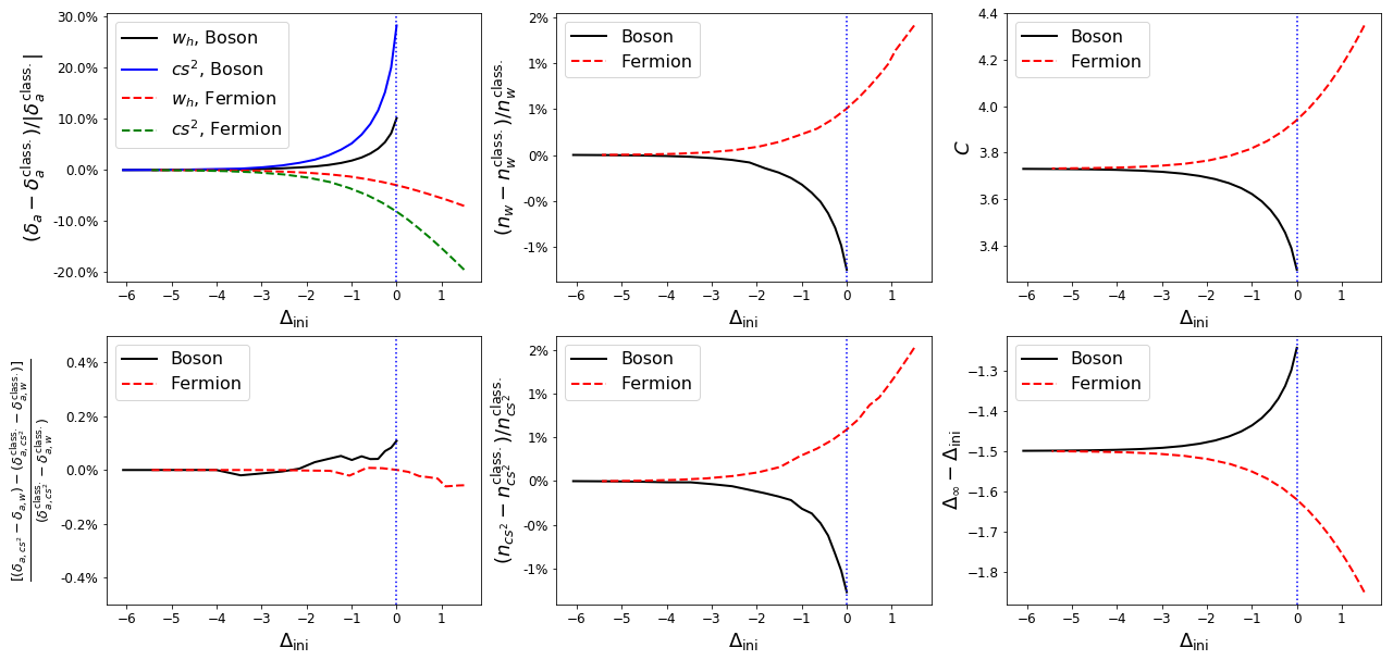
Figure 11: The dependence of the transition on $\Delta_{\rm{ini}}$ and Fermi-Dirac/Bose-Einstein statistics. Although we only consider cases where $\Delta\leq 0$, we include positive $\Delta_{\rm{ini}}$ for the fermion case. Upper left: the transition positions in scale factor relative to $\hat{a}$. These depend on $\Delta_{\rm{ini}}$ for $\Delta_{\rm{ini}}\gtrsim-1$, but in terms of the phenomenology, this dependence is not important. The phenomenologically relevant quantities are the “gap” between the $w_{\rm{h}}$ and the $c_{\rm{s}}^{2}$ transitions and the transition indices $n_{w}$ and $n_{c_{\rm{s}}^{2}}$. As shown in the lower left panel, this “gap” is insensitive to $\Delta_{\rm{ini}}$. Middle: transition indices. Although the transition indices depend on $\Delta_{\rm{ini}}$ more than the “gap” does, their changes are within $2\%$ and hence also insensitive to $\Delta_{\rm{ini}}$. Upper right: the constant $C$ that characterizes the relativistic and nonrelativistic limits of mass over temperature; see Eqs. (2.7) and (2.8). This $C$ depends on $\Delta_{\rm{ini}}$ and quantum statistics, so, when dealing with observations related to the temperature of the HiDM at the nonrelativistic limit we should consider the effects from $\Delta_{\rm{ini}}$ and whether the dark matter is fermionic or bosonic. Lower right: the change in $\Delta$ after the transition. The change is always negative and finite. The fact that $\Delta$ always drops below $-1$ helps explain why the $w_{\rm{h}}$ and $c_{\rm{s}}^{2}$ transitions are insensitive to quantum statistics. See text for detailed discussions.

We can see from Table 2 that the transition depends on the initial effective chemical potential $\Delta_{\rm{ini}}$ and whether the hidden dark matter is fermion or boson. We will now investigate such dependence in more detail. We shall however find that the classical approximation is already very good at representing the transition in all cases.

In Figure 11 we show transition parameters vs. $\Delta_{\rm{ini}}$. We can see that all the transition parameters have their classical limits. They become dependent on $\Delta_{\rm{ini}}$ when $\Delta_{\rm{ini}}\gtrsim-1$. The extent of $\Delta_{\rm{ini}}$ dependence varies for different parameters. For example, the transition scale factors (as expressed relative to the characteristic scale factor $\hat{a}$) can differ from the corresponding classical limits by up to $10\%$ for $w_{\rm{h}}$ and $30\%$ for $\delta p_{\rm h}/\delta\rho_{\rm h}$; this can be seen in the upper left panel of Figure 11. Phenomenologically, however, this dependence should not make much difference. This is because the quantity that affects cosmological observations is the evolution of the energy density, and different $\delta_{a}$’s only shift the transition horizontally which can be transformed away by redefining the transition position. What is important is the “gap” between the $\delta p_{\rm{h}}/\delta\rho_{\rm{h}}$ and the $w_{\rm{h}}$ transitions, i.e., $\delta_{c_{\rm{s}}^{2}}^{a}-\delta_{w}^{a}$. This gap quantifies the delay of the adiabatic sound speed transition as relative to $w_{\rm{h}}$, and it is insensitive to and almost independent of $\Delta_{\rm{ini}}$ or quantum statistics; see the last row in Table 2 and the lower left panel of Figure 11. For the transition indices, the additional degenerate pressure makes the transition slightly sharper (larger indices) for fermions. Opposite effects occur for bosons since the pressure is lower than in the classical case. But the changes are very small. Both transition indices are insensitive to $\Delta_{\rm{ini}}$ or quantum statistics, as shown in the middle panels of Figure 11. For the cosmological observations discussed in this work, the only important time evolution is that of $w_{\rm{h}}$ and $\delta p_{\rm{h}}/\delta\rho_{\rm{h}}$. From the above discussion, it suffices to use the classical limits of the transition parameters to study impacts on cosmological observables, e.g., the CMB power spectra. Therefore we will only use the classical limits of the transition to study the impacts of such hidden dark matter on observations and parameter estimation.

It is also worth discussing the $\Delta_{\rm{ini}}$ dependence of other quantities, e.g., the value of $C$ that characterizes the asymptotic behaviors of the temperature evolution, and the reduction in $\Delta$. As shown in the upper right panel of Figure 11, when $\Delta_{\rm{ini}}\gtrsim-1$, the constant $C$ becomes smaller (larger) for a larger $\Delta_{\rm{ini}}$ for bosons (fermions). This means that for a given initial temperature at the relativistic limit, the temperature will become smaller (larger) than that in the classical case due to bosonic (fermionic) quantum statistics. Take the special case with $\Delta_{\rm{ini}}=0$ for example. The ratio of temperature at the nonrelativistic limit is $3.282/3.922=0.837$ between the boson and the fermion cases. The difference will be smaller for smaller $\Delta_{\rm{ini}}$. The lower right panel shows the change $\Delta_{\rm{ch}}$ vs. $\Delta_{\rm{ini}}\equiv\Delta_{\rm{f}}-\Delta_{\rm{ini}}$. The drop is of order unity but is larger (smaller) due to bosonic (fermionic) quantum statistics when $\Delta_{\rm{ini}}\gtrsim-1$. The amount of reduction in $\Delta$ helps us to see why the transitions of $w_{\rm{h}}$ and $\delta p_{\rm{h}}/\delta\rho_{\rm{h}}$ are rather insensitive to quantum statistics. This is because even if it starts at $0$, $\Delta$ will drop below $-1$ after the transition and largely suppress quantum statistical effects. Thus, the effects from the quantum statistics only appear in a short period of time during the transition.

We have shown the similarity at the background level between the equilibrium case and the free-streaming case in the hidden dark matter model in Sec. 2.1.2 and B.3. Together with the discussions above, we expect that the physical phenomenology for all the considered cases here is similar to each other. We therefore only use the classical case in this work to study the impacts on observations and the corresponding constraints on our model. At the perturbation level, we treat the equilibrium case and free-streaming case differently, which is discussed in Sec. 3.2.

Appendix D Details of the estimation of the constraint from big bang nuclear synthesis element abundance

We use the equilibrium case to calculate the extra radiation energy density at early times. However, since we have seen that the background evolution in the free-streaming case is similar to that of the equilibrium case, we expect that the constraint from BBN is also similar for both cases. In the equilibrium case, the extra radiation energy density in the hidden dark matter scenario is the energy density of the relativistic hidden dark matter. With Eqs. (A.8) and (2.7) we have,

$$\Delta\rho_{\rm{rad}}=\lim_{x\rightarrow 0}\rho_{\rm{h}}=\frac{gm^{4}}{2\pi^{2}\hbar^{3}}\frac{F_{4}^{\mp}(\Delta_{\rm{ini}})}{C^{4}}\frac{\hat{a}^{4}}{a^{4}}\,,$$ (D.1)

where $\Delta_{\rm{ini}}$ is the value of $\Delta$ in the relativistic limit, and the function $F_{s}^{\mp}(\Delta)$ is defined in Eq. (A.10). With Eqs. (A.13) and (2.8), the dark matter energy density in the nonrelativistic phase reads

$$\rho_{\rm{dm}}=\lim_{x\rightarrow\infty}\rho_{\rm{h}}=\frac{gm^{4}}{2\pi\hbar^{3}}\frac{\sqrt{2}F_{3/2}^{\mp}(\Delta_{\infty})}{C^{3/2}}\frac{\hat{a}^{3}}{a^{3}}\,,$$ (D.2)

where $\Delta_{\infty}$ is the value of $\Delta$ in the nonrelativistic limit. The values of $C$, $\Delta_{\rm{ini}}$ and $\Delta_{\infty}$ for some special cases can be found in Table 2. The above two equations give the extra radiation energy density $\Delta\rho_{\rm{rad}}$ in the early universe,

$$\Delta\rho_{\rm{rad}}=\frac{F_{4}^{\mp}(\Delta_{\rm{ini}})\hat{a}\rho_{\rm{m}}^{0}}{\sqrt{2}C^{5/2}F_{3/2}^{\mp}(\Delta_{\infty})a^{4}}\simeq\frac{0.8\,\hat{a}\rho_{\rm{m}}^{0}}{a^{4}}\,,$$ (D.3)

where the approximation is valid for all cases (fermionic or bosonic, regardless of $\Delta_{\rm{ini}}$). For cosmological observations, the extra radiation energy density is usually parameterized with $\Delta N_{\rm{eff}}$ as [5]

$$\Delta\rho_{\rm{rad}}=\Delta N_{\rm{eff}}\times\frac{7}{8}\left(\frac{4}{11}\right)^{4/3}\rho_{\gamma}\,,$$ (D.4)

where $\rho_{\gamma}$ is the energy density of photons. By equating Eqs. (D.3) and (D.4) and using $R_{\rm{eq}}^{\rm{T}}=\hat{a}/a_{\rm{eq}}$ we have

$$R_{\rm{eq}}^{\rm{T}}=0.28\times\frac{\Omega_{\rm{m}}\Omega_{\gamma}}{\Omega_{\rm{dm}}\Omega_{\rm{rad}}}\Delta N_{\rm{eff}}\,,$$ (D.5)

where $\Omega_{\rm{m}}$, $\Omega_{\rm{dm}}$, $\Omega_{\gamma}$ and $\Omega_{\rm{rad}}$ are the density parameters for matter, dark matter, photons, and radiation. Note that $\Omega_{\rm{rad}}$ is calculated by treating neutrinos as relativistic particles. As we shall see, other cosmological constraints on $R_{\rm{eq}}^{\rm{T}}$ are much stronger than the constraint from BBN, so we proceed to only give an estimate of the BBN constraint. We fix all $\Omega$’s to the mean values given in Planck 2018 [5] and adopting a rough upper bound $\Delta N_{\rm{eff}}<1$ [77], we derive an upper bound on $R_{\rm{eq}}^{\rm{T}}$ of

$$R_{\rm{eq}}^{\rm{T}}\lesssim 0.2\,,$$ (D.6)

where the uncertainties of the $\Omega$’s have been ignored.

Appendix E The minimum mass - Jeans mass scales at different redshifts

In section 6.1, we used the Press-Schechter formalism to estimate the halo mass function in the hidden dark matter model. Here we calculate the Jeans mass for dark matter due to its residual velocity dispersion [122]

$$M_{\rm{J,h}}(a,R^{\rm{T}}_{\rm{eq}})=\frac{2.92\times\big{(}c_{\rm{s}}(a)\big{)}^{3}}{G^{3/2}\big{(}\rho_{\rm{m}}(a)\big{)}^{1/2}}=1.1\times 10^{4}\,h^{-1}M_{\odot}\times\Big{(}\frac{R^{\rm{T}}_{\rm{eq}}}{10^{-3}}\Big{)}^{3}a^{-\frac{3}{2}}\,,$$ (E.1)

where the subscript “h” stands for hidden dark matter. We have used Eq. (2.8) with an adiabatic sound speed $c_{\rm{s}}=\big{(}\frac{5}{3}\frac{T}{m}\big{)}^{\frac{1}{2}}=\big{(}\frac{5}{3}\frac{1}{x}\big{)}^{\frac{1}{2}}=\big{(}\frac{5}{3C}\big{)}^{\frac{1}{2}}\frac{\hat{a}}{a}$, and and the classical case constant $C$ from Table 2. This Jeans mass is larger at higher redshifts since the residual temperature was higher. Therefore, such an additional suppression effect is more significant at higher redshifts. For $R_{\rm{eq}}^{\rm{T}}=0.001$, $M_{\rm{J,h}}$ is only $\sim 1.6\times 10^{4}M_{\odot}$ today but is $\sim 2.8\times 10^{6}M_{\odot}$ at $z=30$. The halo mass function at each redshift should be further suppressed when the halo mass is near the corresponding Jeans mass. However, $M_{\rm{J,h}}$ is much lower than $M_{\rm{sup}}$ caused by the suppression of the initial conditions for nonlinear collapse for the same value of $R^{\rm{T}}_{\rm{eq}}$. Therefore, we may neglect this subdominant suppression effect when we calculate the halo mass function in our $\Lambda$HiDM model.

References

- [1] F. Zwicky, Spectral displacement of extra galactic nebulae, Helv. Phys. Acta 6 (1933) 15.
- [2] S. Smith, The mass of the virgo cluster, The Astrophysical Journal 83 (1936) 23.
- [3] H.C. van de Hulst, E. Raimond and H. van Woerden, Rotation and density distribution of the Andromeda nebula derived from observations of the 21-cm line, Bull. Astron. Inst. Netherlands 14 (1957) 1.
- [4] Kirkman et al., The Cosmological Baryon Density from the Deuterium-to-Hydrogen Ratio in QSO Absorption Systems: D/H toward Q1243+3047, ApJS 149 (2003) 1.
- [5] P.A.R. Ade and others (Planck Collaboration), Planck 2018 results. VI. Cosmological parameters, A&A 641 (2020) A6 [1807.06209].
- [6] Dark Energy Survey Collaboration, T.M.C. Abbott et al., Dark Energy Survey year 1 results: Cosmological constraints from galaxy clustering and weak lensing, Phys. Rev. D 98 (2018) 043526 [1708.01530].
- [7] C. Hikage et al., Cosmology from cosmic shear power spectra with Subaru Hyper Suprime-Cam first-year data, Publications of the Astronomical Society of Japan (2019) 22 [1809.09148].
- [8] S. Joudaki et al., KiDS-450 + 2dFLenS: Cosmological parameter constraints from weak gravitational lensing tomography and overlapping redshift-space galaxy clustering, MNRAS 474 (2018) 4894 [1707.06627].
- [9] D. Clowe, M. Bradač, A.H. Gonzalez, M. Markevitch, S.W. Randall, C. Jones et al., A Direct Empirical Proof of the Existence of Dark Matter, ApJ 648 (2006) L109 [astro-ph/0608407].
- [10] W. Lin and M. Ishak, Ultra faint dwarf galaxies: an arena for testing dark matter versus modified gravity, JCAP 10 (2016) 025 [1604.00950].
- [11] H.E.S.S. Collaboration collaboration, Search for -ray line signals from dark matter annihilations in the inner galactic halo from 10 years of observations with h.e.s.s., Phys. Rev. Lett. 120 (2018) 201101.
- [12] AMS Collaboration collaboration, Electron and positron fluxes in primary cosmic rays measured with the alpha magnetic spectrometer on the international space station, Phys. Rev. Lett. 113 (2014) 121102.
- [13] M.H. Chan, L. Cui, J. Liu and C.S. Leung, Ruling out 100-300 GeV Thermal Relic Annihilating Dark Matter by Radio Observation of the Andromeda Galaxy, ApJ 872 (2019) 177 [1901.04638].
- [14] P.F. Depta, M. Hufnagel, K. Schmidt-Hoberg and S. Wild, BBN constraints on the annihilation of MeV-scale dark matter, J. Cosmology Astropart. Phys 2019 (2019) 029 [1901.06944].
- [15] M. Boudaud, T. Lacroix, M. Stref and J. Lavalle, Robust cosmic-ray constraints on p -wave annihilating MeV dark matter, Phys. Rev. D 99 (2019) 061302 [1810.01680].
- [16] S. Schön, K.J. Mack and J.S.B. Wyithe, Dark matter annihilation in the circumgalactic medium at high redshifts, MNRAS 474 (2018) 3067 [1706.04327].
- [17] S. Schön, K.J. Mack, C.A. Avram, J.S.B. Wyithe and E. Barberio, Dark matter annihilation in the first galaxy haloes, MNRAS 451 (2015) 2840 [1411.3783].
- [18] V. Poulin, P.D. Serpico and J. Lesgourgues, A fresh look at linear cosmological constraints on a decaying Dark Matter component, Journal of Cosmology and Astro-Particle Physics 2016 (2016) 036 [1606.02073].
- [19] K. Enqvist, S. Nadathur, T. Sekiguchi and T. Takahashi, Decaying dark matter and the tension in 8, Journal of Cosmology and Astro-Particle Physics 2015 (2015) 067 [1505.05511].
- [20] G. Blackadder and S.M. Koushiappas, Cosmological constraints to dark matter with two- and many-body decays, Phys. Rev. D 93 (2016) 023510 [1510.06026].
- [21] C. Dvorkin, K. Blum and M. Kamionkowski, Constraining dark matter-baryon scattering with linear cosmology, Phys. Rev. D 89 (2014) 023519 [1311.2937].
- [22] L. Visinelli and P. Gondolo, Kinetic decoupling of WIMPs: analytic expressions, Phys. Rev. D 91 (2015) 083526 [1501.02233].
- [23] W.L. Xu, C. Dvorkin and A. Chael, Probing sub-GeV dark matter-baryon scattering with cosmological observables, Phys. Rev. D 97 (2018) 103530 [1802.06788].
- [24] K.K. Boddy, V. Gluscevic, V. Poulin, E.D. Kovetz, M. Kamionkowski and R. Barkana, Critical assessment of CMB limits on dark matter-baryon scattering: New treatment of the relative bulk velocity, Phys. Rev. D 98 (2018) 123506 [1808.00001].
- [25] J. Ooba, H. Tashiro and K. Kadota, Cosmological constraints on the velocity-dependent baryon-dark matter coupling, arXiv e-prints (2019) arXiv:1902.00826 [1902.00826].
- [26] R. Barkana, N.J. Outmezguine, D. Redigol and T. Volansky, Strong constraints on light dark matter interpretation of the EDGES signal, Phys. Rev. D 98 (2018) 103005 [1803.03091].
- [27] E.O. Nadler, V. Gluscevic, K.K. Boddy and R.H. Wechsler, Constraints on Dark Matter Microphysics from the Milky Way Satellite Population, ApJ 878 (2019) L32 [1904.10000].
- [28] Cosine-100 Collaboration, G. Adhikari et al., An experiment to search for dark-matter interactions using sodium iodide detectors, Nature 564 (2018) 83 [1906.01791].
- [29] G. Beck, An excess of excesses examined via dark matter radio emissions from galaxies, J. Cosmology Astropart. Phys 2019 (2019) 019 [1905.05599].
- [30] CRESST collaboration, F. Petricca et al., First results on low-mass dark matter from the CRESST-III experiment, arXiv e-prints (2017) arXiv:1711.07692 [1711.07692].
- [31] LUX Collaboration, D.S. Akerib et al., Results from a Search for Dark Matter in the Complete LUX Exposure, Phys. Rev. Lett. 118 (2017) 021303 [1608.07648].
- [32] Xenon Collaboration, E. Aprile et al., Low-mass dark matter search using ionization signals in XENON100, Phys. Rev. D 94 (2016) 092001 [1605.06262].
- [33] Xenon Collaboration, E. Aprile et al., First Dark Matter Search Results from the XENON1T Experiment, Phys. Rev. Lett. 119 (2017) 181301 [1705.06655].
- [34] E.D. Carlson, M.E. Machacek and L.J. Hall, Self-interacting dark matter, ApJ 398 (1992) 43.
- [35] P. Bode, J.P. Ostriker and N. Turok, Halo formation in warm dark matter models, The Astrophysical Journal 556 (2001) 93.
- [36] M. Viel, G.D. Becker, J.S. Bolton, M.G. Haehnelt, M. Rauch and W.L.W. Sargent, How cold is cold dark matter? small-scales constraints from the flux power spectrum of the high-redshift lyman- forest, Phys. Rev. Lett. 100 (2008) 041304.
- [37] M. Safarzadeh, E. Scannapieco and A. Babul, A Limit on the Warm Dark Matter Particle Mass from the Redshifted 21 cm Absorption Line, ApJ 859 (2018) L18 [1803.08039].
- [38] A. Boyarsky, D. Iakubovskyi, O. Ruchayskiy, A. Rudakovskyi and W. Valkenburg, 21-cm observations and warm dark matter models, Phys. Rev. D 100 (2019) 123005 [1904.03097].
- [39] P.S. Bhupal Dev, A. Mazumdar and S. Qutub, Constraining Non-thermal and Thermal properties of Dark Matter, Front. in Phys. 2 (2014) 26 [1311.5297].
- [40] M.A.G. Garcia, K. Kaneta, Y. Mambrini and K.A. Olive, Reheating and post-inflationary production of dark matter, Phys. Rev. D 101 (2020) 123507.
- [41] A.L. Erickcek, P. Ralegankar and J. Shelton, Cannibal domination and the matter power spectrum, Phys. Rev. D 103 (2021) 103508 [2008.04311].
- [42] C. Miller, A.L. Erickcek and R. Murgia, Constraining nonthermal dark matter’s impact on the matter power spectrum, Phys. Rev. D 100 (2019) 123520 [1908.10369].
- [43] C. Blanco, M.S. Delos, A.L. Erickcek and D. Hooper, Annihilation signatures of hidden sector dark matter within early-forming microhalos, Phys. Rev. D 100 (2019) 103010 [1906.00010].
- [44] G. Bertone and T.M.P. Tait, A new era in the search for dark matter, Nature 562 (2018) 51 [1810.01668].
- [45] M. Battaglieri et al., US Cosmic Visions: New Ideas in Dark Matter 2017: Community Report, arXiv e-prints (2017) arXiv:1707.04591 [1707.04591].
- [46] B.W. Lee and S. Weinberg, Cosmological lower bound on heavy-neutrino masses, Phys. Rev. Lett. 39 (1977) 165.
- [47] D.A. Dicus, E.W. Kolb and V.L. Teplitz, Cosmological upper bound on heavy-neutrino lifetimes, Phys. Rev. Lett. 39 (1977) 168.
- [48] S. Dodelson and L.M. Widrow, Sterile neutrinos as dark matter, Phys. Rev. Lett. 72 (1994) 17 [hep-ph/9303287].
- [49] S. Colombi, S. Dodelson and L.M. Widrow, Large-Scale Structure Tests of Warm Dark Matter, ApJ 458 (1996) 1 [astro-ph/9505029].
- [50] M. Viel, J. Lesgourgues, M.G. Haehnelt, S. Matarrese and A. Riotto, Constraining warm dark matter candidates including sterile neutrinos and light gravitinos with WMAP and the Lyman- forest, Phys. Rev. D 71 (2005) 063534 [astro-ph/0501562].
- [51] X. Chen and S.-H.H. Tye, Heating in brane inflation and hidden dark matter, J. Cosmology Astropart. Phys 6 (2006) 011 [hep-th/0602136].
- [52] R. Allahverdi and M. Drees, Production of massive stable particles in inflaton decay, Phys. Rev. Lett. 89 (2002) 091302 [hep-ph/0203118].
- [53] R. Allahverdi and M. Drees, Thermalization after inflation and production of massive stable particles, Phys. Rev. D 66 (2002) 063513 [hep-ph/0205246].
- [54] A. Berlin, D. Hooper and G. Krnjaic, PeV-scale dark matter as a thermal relic of a decoupled sector, Physics Letters B 760 (2016) 106 [1602.08490].
- [55] C. Blanco, M.S. Delos, A.L. Erickcek and D. Hooper, Annihilation signatures of hidden sector dark matter within early-forming microhalos, Phys. Rev. D 100 (2019) 103010 [1906.00010].
- [56] A.L. Erickcek, The dark matter annihilation boost from low-temperature reheating, Phys. Rev. D 92 (2015) 103505 [1504.03335].
- [57] D. Feldman, B. Kors and P. Nath, Extra-weakly Interacting Dark Matter, Phys. Rev. D 75 (2007) 023503 [hep-ph/0610133].
- [58] D. Feldman, Z. Liu and P. Nath, The Stueckelberg extension and milli weak and milli charged dark matter, AIP Conf. Proc. 939 (2007) 50 [0705.2924].
- [59] J.L. Feng and J. Kumar, The WIMPless Miracle: Dark-Matter Particles without Weak-Scale Masses or Weak Interactions, Phys. Rev. Lett. 101 (2008) 231301 [0803.4196].
- [60] J.L. Feng, H. Tu and H.-B. Yu, Thermal Relics in Hidden Sectors, JCAP 10 (2008) 043 [0808.2318].
- [61] X. Chen, Decaying Hidden Dark Matter in Warped Compactification, JCAP 09 (2009) 029 [0902.0008].
- [62] W. Lin, L. Visinelli, D. Xu and T.T. Yanagida, Neutrino astronomy as a probe of physics beyond the Standard Model: Decay of sub-MeV B-L gauge boson dark matter, Phys. Rev. D 106 (2022) 075011 [2202.04496].
- [63] W. Lin and T.T. Yanagida, Confronting the Galactic 511 keV emission with B-L gauge boson dark matter, Phys. Rev. D 106 (2022) 075012 [2205.08171].
- [64] W. Hu, Structure Formation with Generalized Dark Matter, ApJ 506 (1998) 485 [astro-ph/9801234].
- [65] M. Kopp, C. Skordis and D.B. Thomas, Extensive investigation of the generalized dark matter model, Phys. Rev. D 94 (2016) 043512 [1605.00649].
- [66] M. Kopp, C. Skordis, D.B. Thomas and S. Ilić, Dark Matter Equation of State through Cosmic History, Phys. Rev. Lett. 120 (2018) 221102 [1802.09541].
- [67] S. Kumar, R.C. Nunes and S.K. Yadav, Testing the warmness of dark matter, MNRAS 490 (2019) 1406 [1901.07549].
- [68] A.G. Riess, S. Casertano, W. Yuan, L.M. Macri and D. Scolnic, Large Magellanic Cloud Cepheid Standards Provide a 1% Foundation for the Determination of the Hubble Constant and Stronger Evidence for Physics beyond CDM, ApJ 876 (2019) 85 [1903.07603].
- [69] J.R. Bond, G. Efstathiou and J. Silk, Massive neutrinos and the large-scale structure of the universe, Phys. Rev. Lett. 45 (1980) 1980.
- [70] A. Schneider, R.E. Smith and D. Reed, Halo mass function and the free streaming scale, Monthly Notices of the Royal Astronomical Society 433 (2013) 1573.
- [71] W.S. Hipólito-Ricaldi, R.F. vom Marttens, J.C. Fabris, I.L. Shapiro and L. Casarini, On general features of warm dark matter with reduced relativistic gas, European Physical Journal C 78 (2018) 365 [1706.08595].
- [72] G. de Berredo-Peixoto, I.L. Shapiro and F. Sobreira, Simple Cosmological Model with Relativistic Gas, Modern Physics Letters A 20 (2005) 2723 [gr-qc/0412050].
- [73] A. Lewis and A. Challinor, Evolution of cosmological dark matter perturbations, Phys. Rev. D 66 (2002) 023531 [astro-ph/0203507].
- [74] H. Ganjoo, A.L. Erickcek, W. Lin and K.J. Mack, The Effects Of Relativistic Hidden Sector Particles on the Matter Power Spectrum, arXiv e-prints (2022) arXiv:2209.02735 [2209.02735].
- [75] A. Das, B. Dasgupta and R. Khatri, Ballistic Dark Matter oscillates above CDM, J. Cosmology Astropart. Phys 2019 (2019) 018 [1811.00028].
- [76] R.J. Cooke, M. Pettini and C.C. Steidel, One Percent Determination of the Primordial Deuterium Abundance, ApJ 855 (2018) 102 [1710.11129].
- [77] Y.I. Izotov, T.X. Thuan and N.G. Guseva, A new determination of the primordial He abundance using the He I 10830 Å emission line: cosmological implications, MNRAS 445 (2014) 778 [1408.6953].
- [78] C.-P. Ma and E. Bertschinger, Cosmological Perturbation Theory in the Synchronous and Conformal Newtonian Gauges, ApJ 455 (1995) 7 [astro-ph/9506072].
- [79] S. Weinberg, Cosmology, Oxford University Press, New York (2008).
- [80] G. Ellis, R. Treciokas and D. Matravers, Anisotropic solutions of the einstein-boltzmann equations. ii. some exact properties of the equations, Annals of Physics 150 (1983) 487 .
- [81] T. Tenkanen, Dark Matter from Scalar Field Fluctuations, Phys. Rev. Lett. 123 (2019) 061302 [1905.01214].
- [82] Y. Akrami and others (Planck Collaboration), Planck 2018 results. X. Constraints on inflation, A&A 641 (2020) A10 [1807.06211].
- [83] A. Lewis, A. Challinor and A. Lasenby, Efficient computation of cosmic microwave background anisotropies in closed friedmann-robertson-walker models, The Astrophysical Journal 538 (2000) 473.
- [84] A. Lewis and S. Bridle, Cosmological parameters from CMB and other data: A Monte Carlo approach, Phys. Rev. D 66 (2002) 103511 [astro-ph/0205436].
- [85] C.M. Müller, Cosmological bounds on the equation of state of dark matter, Phys. Rev. D 71 (2005) 047302 [astro-ph/0410621].
- [86] E. Calabrese, M. Migliaccio, L. Pagano, G. de Troia, A. Melchiorri and P. Natoli, Cosmological constraints on the matter equation of state, Phys. Rev. D 80 (2009) 063539.
- [87] M. Kopp, C. Skordis, D.B. Thomas and S. Ilić, Dark Matter Equation of State through Cosmic History, Phys. Rev. Lett. 120 (2018) 221102 [1802.09541].
- [88] M. Bucher, K. Moodley and N. Turok, General primordial cosmic perturbation, Phys. Rev. D 62 (2000) 083508 [astro-ph/9904231].
- [89] Planck Collaboration, P.A.R. Ade et al., Planck 2013 results. XXII. Constraints on inflation, A&A 571 (2014) A22 [1303.5082].
- [90] C. Heymans et al., CFHTLenS: the Canada-France-Hawaii Telescope Lensing Survey, MNRAS 427 (2012) 146 [1210.0032].
- [91] W.L. Xu, J.B. Muñoz and C. Dvorkin, Cosmological Constraints on Light (but Massive) Relics, arXiv e-prints (2021) arXiv:2107.09664 [2107.09664].
- [92] P. McDonald et al., The Ly Forest Power Spectrum from the Sloan Digital Sky Survey, The Astrophysical Journal Supplement Series 163 (2006) 80 [astro-ph/0405013].
- [93] M. Viel, J. Weller and M.G. Haehnelt, Constraints on the primordial power spectrum from high-resolution Lyman forest spectra and WMAP, MNRAS 355 (2004) L23 [astro-ph/0407294].
- [94] M. Viel, M.G. Haehnelt and A. Lewis, The Lyman forest and WMAP year three, MNRAS 370 (2006) L51 [astro-ph/0604310].
- [95] W.H. Press and P. Schechter, Formation of Galaxies and Clusters of Galaxies by Self-Similar Gravitational Condensation, ApJ 187 (1974) 425.
- [96] J.R. Bond, S. Cole, G. Efstathiou and N. Kaiser, Excursion set mass functions for hierarchical Gaussian fluctuations, ApJ 379 (1991) 440.
- [97] R.G. Bower, The evolution of groups of galaxies in the Press–Schechter formalism, Monthly Notices of the Royal Astronomical Society 248 (1991) 332.
- [98] C. Lacey and S. Cole, Merger rates in hierarchical models of galaxy formation, MNRAS 262 (1993) 627.
- [99] R.K. Sheth and G. Tormen, An excursion set model of hierarchical clustering: ellipsoidal collapse and the moving barrier, MNRAS 329 (2002) 61 [astro-ph/0105113].
- [100] A.D. Ludlow, S. Bose, R.E. Angulo, L. Wang, W.A. Hellwing, J.F. Navarro et al., The mass-concentration-redshift relation of cold and warm dark matter haloes, MNRAS 460 (2016) 1214 [1601.02624].
- [101] A.J. Benson, A. Farahi, S. Cole, L.A. Moustakas, A. Jenkins, M. Lovell et al., Dark matter halo merger histories beyond cold dark matter - I. Methods and application to warm dark matter, MNRAS 428 (2013) 1774 [1209.3018].
- [102] V. Avila-Reese, P. Colin, O. Valenzuela, E. D’Onghia and C. Firmani, Formation and structure of halos in a warm dark matter cosmology, The Astrophysical Journal 559 (2001) 516.
- [103] A.V. Macciò, O. Ruchayskiy, A. Boyarsky and J.C. Muñoz-Cuartas, The inner structure of haloes in cold+warm dark matter models, MNRAS 428 (2013) 882 [1202.2858].
- [104] D. Gilman, S. Birrer, A. Nierenberg, T. Treu, X. Du and A. Benson, Warm dark matter chills out: constraints on the halo mass function and the free-streaming length of dark matter with eight quadruple-image strong gravitational lenses, MNRAS 491 (2020) 6077 [1908.06983].
- [105] E.O. Nadler, Y.-Y. Mao, G.M. Green and R.H. Wechsler, Modeling the connection between subhalos and satellites in milky way–like systems, The Astrophysical Journal 873 (2019) 34.
- [106] P. Jethwa, D. Erkal and V. Belokurov, The upper bound on the lowest mass halo, Mon. Not. Roy. Astron. Soc. 473 (2018) 2060 [1612.07834].
- [107] O. Newton, M. Leo, M. Cautun, A. Jenkins, C.S. Frenk, M.R. Lovell et al., Constraints on the properties of warm dark matter using the satellite galaxies of the Milky Way, arXiv e-prints (2020) arXiv:2011.08865 [2011.08865].
- [108] W. Enzi, R. Murgia, O. Newton, S. Vegetti, C. Frenk, M. Viel et al., Joint constraints on thermal relic dark matter from strong gravitational lensing, the Lyman- forest, and Milky Way satellites, MNRAS (2021) [2010.13802].
- [109] J. Bowman, A. Rogers, R. Monsalve, T. Mozdzen and N. Mahesh, An absorption profile centred at 78 megahertz in the sky-averaged spectrum, Nature 555 (2018) 67.
- [110] L. Lopez-Honorez, O. Mena, S. Palomares-Ruiz and P. Villanueva-Domingo, Warm dark matter and the ionization history of the Universe, Phys. Rev. D 96 (2017) 103539 [1703.02302].
- [111] C. Destri, H.J. de Vega and N.G. Sanchez, Quantum WDM fermions and gravitation determine the observed galaxy structures, Astroparticle Physics 46 (2013) 14 [1301.1864].
- [112] P.-H. Chavanis, M. Lemou and F. Méhats, Models of dark matter halos based on statistical mechanics: The classical King model, Phys. Rev. D 91 (2015) 063531 [1409.7838].
- [113] P.-H. Chavanis, M. Lemou and F. Méhats, Models of dark matter halos based on statistical mechanics: The fermionic King model, Phys. Rev. D 92 (2015) 123527 [1409.7840].
- [114] W. Hu, R. Barkana and A. Gruzinov, Fuzzy cold dark matter: The wave properties of ultralight particles, Phys. Rev. Lett. 85 (2000) 1158.
- [115] A. Burkert, Fuzzy dark matter and dark matter halo cores, The Astrophysical Journal 904 (2020) 161.
- [116] H. Deng, M.P. Hertzberg, M.H. Namjoo and A. Masoumi, Can light dark matter solve the core-cusp problem?, Phys. Rev. D 98 (2018) 023513.
- [117] D.C. Rodrigues, A. del Popolo, V. Marra and P.L.C. de Oliveira, Evidence against cuspy dark matter haloes in large galaxies, MNRAS 470 (2017) 2410 [1701.02698].
- [118] R. Kennedy, C. Frenk, S. Cole and A. Benson, Constraining the warm dark matter particle mass with Milky Way satellites, MNRAS 442 (2014) 2487 [1310.7739].
- [119] M. Kaplinghat, T. Ren and H.-B. Yu, Dark matter cores and cusps in spiral galaxies and their explanations, Journal of Cosmology and Astroparticle Physics 2020 (2020) .
- [120] S. Tulin and H.-B. Yu, Dark matter self-interactions and small scale structure, Physics Reports 730 (2018) 1 .
- [121] W.-W. Tan, F.Y. Wang and K.S. Cheng, Constraining Warm Dark Matter Mass with Cosmic Reionization and Gravitational Waves, ApJ 829 (2016) 29 [1607.03567].
- [122] J. Binney and S. Tremaine, Galactic Dynamics: Second Edition, Princeton Series in Astrophysics, Princeton University Press (2011).