Potential renormalisation, Lamb shift and mean-force Gibbs state—to shift or not to shift?

Abstract

An open system, even if coupled weakly to a bath, can experience a non-negligible potential renormalisation, quantified by the ‘reorganisation energy’. Often, the microscopic system–bath coupling gives rise to a counter term which adds to the bare Hamiltonian, exactly compensating for such potential distortion. On the other hand, when describing quantum dissipative dynamics with weak-coupling master equations, a number of ‘Lamb-shift terms’ appear which, contrary to popular belief, cannot be neglected. And yet, the practice of vanishing both the counter term and Lamb-shift contributions is almost universal; and, surprisingly, it gives excellent results. In this paper we use a damped quantum harmonic oscillator to analytically show that subtracting the reorganisation energy from the Hamiltonian and then suppressing the Lamb-shift terms from the resulting master equation, does indeed yield an excellent approximation to the exact steady state and long-time dynamics. Put differently, those seemingly unjustified steps succeed at building the asymptotic mean-force Gibbs state—or rather, its classical limit—into the master equation. This can noticeably increase its accuracy, specially at moderate-to-low temperatures and even up to intermediate coupling. We thus shed light on an overlooked issue that becomes critical in the calculation of heat currents in quantum thermodynamics.

I Introduction

Markovian master equations lay at the root of quantum thermodynamics Alicki and Kosloff (2018). They can approximate the state of an open system weakly coupled to various heat baths, and allow for the definition of thermodynamically consistent heat currents Alicki (1979); Geva and Kosloff (1992). In turn, this enables the design of quantum heat engines and refrigerators Kosloff and Levy (2014); Ghosh et al. (2018), some of which have already found experimental realisation in a variety of platforms Zou et al. (2017); Brantut et al. (2013); Roßnagel et al. (2016); von Lindenfels et al. (2019); Thierschmann et al. (2015); Klatzow et al. (2019). Crucially, any approximations affecting the structure of master equations can have a major impact on any subsequent thermodynamic analysis. Hence, they need to be justified carefully.

Specifically, let us think of an open system with Hamiltonian $\boldsymbol{H}=\boldsymbol{H}_{S}+\boldsymbol{H}_{B}+\boldsymbol{V}$, where the terms denote system, bath, and system–bath coupling, respectively. Here, and in what follows, operators will be denoted by boldface symbols. Assuming that the bath is initially in equilibrium at inverse temperature $\beta=1/k\,T$, i.e., $\boldsymbol{\varrho}_{B}(0)=e^{-\beta\,\boldsymbol{H}_{B}}/\operatorname{tr}_{B}{e^{-\beta\,\boldsymbol{H}_{B}}}=\boldsymbol{\pi}_{B}$, the system is generally assumed to evolve towards the mean-force Gibbs state $\boldsymbol{\tau}_{MF}=\operatorname{tr}_{B}e^{-\beta\,\boldsymbol{H}}/\operatorname{tr}e^{-\beta\,\boldsymbol{H}}$ Onsager (1933); Jarzynski (2004); Trushechkin et al. (2022); Subaş ı et al. (2012). For a linear bath, the classical limit of $\boldsymbol{\tau}_{MF}$ is Cerisola et al. (2022); Cresser and Anders (2021); Timofeev and Trushechkin (2022)

$$\boldsymbol{\tau}_{MF}(\beta\ll\omega_{0})\simeq\frac{e^{-\beta\,(\boldsymbol{H}_{S}-Q\,\boldsymbol{S}^{2})}}{\operatorname{tr}_{S}{e^{-\beta\,(\boldsymbol{H}_{S}-Q\,\boldsymbol{S}^{2})}}},$$ (1)

where we cast $\boldsymbol{V}=\boldsymbol{S}\otimes\boldsymbol{B}$ as the product of a system and a bath operator, and $Q$ is the reorganisation energy Wu et al. (2010); Ritschel et al. (2011). From now on, we shall also take $\hbar=k=1$. Eq. (1) differs from the local thermal state $\boldsymbol{\pi}_{S}=e^{-\beta\,\boldsymbol{H}_{S}}/\operatorname{tr}_{S}{e^{-\beta\,\boldsymbol{H}_{S}}}$ due to the distortion of the potential of the system caused by the finite coupling to the bath Weiss (2008). Whenever such renormalisation effect is not physically expected we redefine $\boldsymbol{H}_{S}=\boldsymbol{H}_{S}^{(0)}+Q\,\boldsymbol{S}^{2}$, which includes a counter-term neutralising the distortion Caldeira and Leggett (1983). The bare Hamiltonian (i.e., that of the system in isolation) is denoted here as $\boldsymbol{H}_{S}^{(0)}$. Adding this term to the model ad hoc has clear advantages. Namely, it keeps us from mistaking the potential renormalisation for dissipative effects Caldeira and Leggett (1983). Furthermore, the counter term ensures that the potential remains confining even at strong coupling Weiss (2008). However, one must bear in mind that, when present, this correction arises naturally from the microscopic coupling. It is thus an integral part of the physical Hamiltonian of the open system Caldeira and Leggett (1983).

Notwithstanding all the above, when deriving weak-coupling master equations the counter term is systematically ignored Correa et al. (2019). Other than in the trivial case $\boldsymbol{S}^{2}\,\propto\,\mathbbm{1}$, such omission is questionable; especially if $Q$ is comparable to the characteristic energies of the system. As we shall see, this may indeed be the case even when the system–bath coupling is perturvatively weak. On its own, this omission leads to an incorrect identification of the decay channels of the open system and, ultimately, to a misrepresentation of the heat currents.

Likewise, several terms are customarily removed from the Markovian master equation—specifically, the non-secular Born–Markov Redfield equation Redfield (1957, 1965). These are the so-called Lamb-shift terms, which contribute both to an effective renormalisation of the system and to purely dissipative processes Cresser and Facer (2017). In order to justify this, one typically argues that the Lamb shift is negligible. Unfortunately, this is not true in general Winczewski and Alicki (2021). We thus find ourselves in the paradoxical situation that two seemingly unjustified manipulations can yield excellent numerical results when combined. In this paper we set out to clarify why. To do so, we exploit the simplicity of an exactly solvable damped harmonic oscillator.

Specifically, we find that

1. renormalising the system Hamiltonian $\boldsymbol{H}_{S}$ by subtracting the reorganisation energy $Q\,\boldsymbol{S}^{2}$ from it,

2. deriving a Born–Markov Redfield equation from such renormalised Hamiltonian,

3. and removing all Lamb-shift terms from the resulting Redfield equation,

can yield an accurate representation of the long-time dynamics. Provided that the secular approximation is justified, it eventually brings the equation above into the standard Davies or Gorini–Kossakowski–Lindblad–Sudarshan (GKLS) form Davies (1974); Gorini et al. (1976); Lindblad (1976), which is most commonly used.

We analytically show how, after undertaking these steps, our model is driven towards the classical limit of $\boldsymbol{\tau}_{MF}$ in Eq. (1). We further show that this limiting case is remarkably close to the exact mean-force Gibbs state over a broad range of parameters, which extends far beyond the high-temperature (classical) regime. More generally, these manipulations yield the correct high-temperature steady state on arbitrary open systems for which the secular approximation is justified. Also, in the adiabatic limit, the transient oscillations are well captured by this simple artefact. Hence, rather than proposing new master-equation techniques, we provide an explanation for the unlikely success of the standard procedure, and clarify some common misconceptions about its justification.

This paper is organised as follows. In Sec. II we introduce our model and discuss the potential renormalisation effect and the corresponding counter term. Then, in Sec. III, we turn our attention to the Born–Markov quantum master equation in detail. Specifically, in Secs. III.2 and III.3 we establish a link between reorganisation energy and Lamb-shift terms of the master equation, and discuss the impact of the secular approximation. Next, we present our main arguments regarding the renormalisation of the Hamiltonian and the removal of Lamb-shift terms, as well as the approximation of the mean-force Gibbs state by its classical limit (cf. Sec. III.4). Before illustrating our results in Sec. V, we outline the exact solution of our model in Sec. IV (details can be found in Appendix B). Finally, in Sec. VI we draw our conclusions.

II Potential renormalisation

Let us consider a harmonic oscillator with Hamiltonian

$$\boldsymbol{H}_{S}^{(0)}=\frac{1}{2}\omega_{0}^{2}\,\boldsymbol{x}^{2}+\frac{1}{2}\,\boldsymbol{p}^{2}$$ (2)

and mass $m=1$. The system is coupled to the linear bath $\boldsymbol{H}_{B}=\sum\nolimits_{\mu}\omega_{\mu}^{2}m_{\mu}\boldsymbol{x}_{\mu}^{2}/2+\boldsymbol{p}_{\mu}^{2}/(2m_{\mu})$ through

$$\boldsymbol{V}=\boldsymbol{x}\otimes\sum\nolimits_{\mu}g_{\mu}\boldsymbol{x}_{\mu}=\boldsymbol{x}\otimes\boldsymbol{B}.$$ (3)

The couplings $g_{\mu}$ are set by the the spectral density $J(\omega)=\pi\,\sum\nolimits_{\mu}g_{\mu}^{2}/(2m_{\mu}\omega_{\mu})\,\delta(\omega-\omega_{\mu})$ which, in our case, is given by

$$J(\omega)=\frac{\lambda\,\omega}{1+(\omega/\Lambda)^{2}}.$$ (4)

As already advanced, our system evolves towards the mean-force Gibbs state $\boldsymbol{\tau}_{MF}$, whose high-temperature limit is

$$\boldsymbol{\tau}_{MF}(\beta\ll\omega_{0})\simeq\frac{e^{-\beta\left[\frac{1}{2}(\omega_{0}^{2}-\Delta\omega^{2})\,\boldsymbol{x}^{2}+\frac{1}{2}\,\boldsymbol{p}^{2}\right]}}{\operatorname{tr}_{S}\,e^{-\beta\left[\frac{1}{2}(\omega_{0}^{2}-\Delta\omega^{2})\,\boldsymbol{x}^{2}+\frac{1}{2}\,\boldsymbol{p}^{2}\right]}}.$$ (5)

This is the thermal state of an oscillator in a modified harmonic potential at the temperature of the bath. The frequency shift is $\Delta\omega^{2}=\frac{1}{\pi}\int_{-\infty}^{\infty}d\omega\,J(\omega)/\omega$, and the term $-\frac{1}{2}\,\Delta\omega^{2}\,\boldsymbol{x}^{2}$ is thus the reorganisation energy. Importantly, this shift is not necessarily small compared with $\omega_{0}^{2}$, even if the system–bath coupling $\lambda$ is weak Correa et al. (2019); Winczewski and Alicki (2021). For instance, $\Delta\omega^{2}=\lambda\Lambda$ for the $J(\omega)$ in Eq. (4). Hence, one can easily find $\Delta\omega^{2}$ comparable to $\omega_{0}^{2}$, especially in the adiabatic limit of $\omega_{0}/\Lambda\ll 1$.

III Born–Markov master equations

III.1 Redfield equation

Having introduced our model, let us tackle its dynamics. Assuming that the strength $\lambda$ of the system–bath coupling is weak, we may approximate the time evolution through the “Markovian” Redfield quantum master equation Breuer and Petruccione (2002)

$$\frac{d\widetilde{\boldsymbol{\varrho}}_{S}}{dt}=-\int_{0}^{\infty}ds\,\operatorname{tr}_{B}\,[\widetilde{\boldsymbol{V}}(t),\,[\widetilde{\boldsymbol{V}}(t-s),\,\widetilde{\boldsymbol{\varrho}}_{S}(t)\otimes\boldsymbol{\pi}_{B}]],$$ (6)

where $\boldsymbol{\varrho}(0)=\boldsymbol{\varrho}_{S}(0)\otimes\boldsymbol{\pi}_{B}$. Hence, $\langle\boldsymbol{B}\rangle_{B}=\operatorname{tr}_{B}[\boldsymbol{B}\,\boldsymbol{\varrho}(0)]=0$, so that the master equation is homogeneous

Owing to the Born approximation, the global state can be assumed to factorise also at $t>0$ (i.e., $\boldsymbol{\varrho}(t)\simeq\boldsymbol{\varrho}_{S}(t)\otimes\boldsymbol{\pi}_{B}$), while the Born–Markov approximation allows for the time-local structure of Eq. (6). Here, $\widetilde{\boldsymbol{O}}(t)=e^{i\,\boldsymbol{H}_{0}\,t}\,\boldsymbol{O}\,e^{-i\,\boldsymbol{H}_{0}\,t}$ denotes interaction picture with respect to $\boldsymbol{H}_{0}=\boldsymbol{H}_{S}+\boldsymbol{H}_{B}$, and $[\bullet,\bullet]$ is a commutator. We stress that, by default, we use $\boldsymbol{H}_{S}$ and $\boldsymbol{H}_{S}^{(0)}$ interchangeably. However, when explicitly stated, $\boldsymbol{H}_{S}$ will stand for $\boldsymbol{H}_{S}^{(0)}\pm\frac{1}{2}\Delta\omega^{2}\,\boldsymbol{x}^{2}$.

We can separate the coherent contributions to the open dynamics by bringing Eq. (6) into the form $d\widetilde{\boldsymbol{\varrho}}_{S}/dt=-i\,[\widetilde{\Delta\boldsymbol{H}},\,\widetilde{\boldsymbol{\varrho}}_{S}]+\widetilde{\pazocal{R}}(t)\,\widetilde{\boldsymbol{\varrho}}_{S}$ (see, e.g., Refs. Cattaneo et al. (2019); Winczewski and Alicki (2021); Timofeev and Trushechkin (2022)), where the Hamiltonian correction $\widetilde{\Delta\boldsymbol{H}}$ is

$$\widetilde{\Delta\boldsymbol{H}}=-\frac{i}{2}\,\int_{0}^{\infty}ds\,\operatorname{tr}_{B}\,\left([\widetilde{\boldsymbol{V}}(t),\,\widetilde{\boldsymbol{V}}(t-s)]\,\boldsymbol{\varrho}_{B}\right),$$ (7)

and the superoperator $\pazocal{R}$ is explicitly written in Sec. III.3 below. Finally, moving to the Schrödinger picture gives

$$\frac{d\boldsymbol{\varrho}_{S}}{dt}=-i[\boldsymbol{H}_{S}+\Delta\boldsymbol{H},\,\boldsymbol{\varrho}_{S}]+\pazocal{R}\,\boldsymbol{\varrho}_{S}(t),$$ (8)

III.2 Lamb shift and reorganisation energy

The effective correction to our system’s Hamiltonian is

$$\Delta\boldsymbol{H}=-\frac{1}{2}\,\Sigma^{\prime}\,\boldsymbol{x}^{2}+\frac{\Delta^{\prime}}{4\omega_{0}}-\frac{\Delta}{8\,\omega_{0}}\,\{\boldsymbol{x},\,\boldsymbol{p}\},$$ (9)

where the notations $\Delta$, $\Delta^{\prime}$ and $\Sigma^{\prime}$ are

$$\Delta =-2\,J(\omega_{0}),$$ (10a)

$$\Sigma^{\prime} =\frac{1}{\pi}~{}\mathchoice{{\vbox{\hbox{$\textstyle-$}}\kern-4.86108pt}}{{\vbox{\hbox{$\scriptstyle-$}}\kern-3.25pt}}{{\vbox{\hbox{$\scriptscriptstyle-$}}\kern-2.29166pt}}{{\vbox{\hbox{$\scriptscriptstyle-$}}\kern-1.875pt}}\!\int_{-\infty}^{\infty}d\omega\,\frac{J(\omega)}{\omega-\omega_{0}}=\pazocal{H}\,J(\omega_{0}),$$ (10b)

$$\Delta^{\prime} =-\pazocal{H}\left[J(\omega_{0})\,\left(2\,n(\omega_{0})+1\right)\right],$$ (10c)

$n(\omega)=(e^{\beta\omega}-1)^{-1}$ is the bosonic occupation, $\mathchoice{{\vbox{\hbox{$\textstyle-$}}\kern-4.86108pt}}{{\vbox{\hbox{$\scriptstyle-$}}\kern-3.25pt}}{{\vbox{\hbox{$\scriptscriptstyle-$}}\kern-2.29166pt}}{{\vbox{\hbox{$\scriptscriptstyle-$}}\kern-1.875pt}}\!\int$ stands for Cauchy principal value, $\pazocal{H}$, for Hilbert transform Bateman (1954), and $\{\bullet,\bullet\}$, for anti-commutator. These formulas also assume that the spectral density is extended as an odd function for negative frequencies, i.e., $J(\omega)=-J(-\omega)$. Importantly, the variables introduced in Eqs. (10) relate to the decay rate $\gamma(\omega)$ and Lamb shift $S(\omega)$ Breuer and Petruccione (2002)

$$\gamma(\omega) =2\,J(\omega)\,(1+n(\omega)),$$

$$S(\omega) =-\pazocal{H}\,[J(\omega)\,\left(n(\omega)+1\right)],$$

which are the real and imaginary parts of the Laplace transform of the bath correlation function $\langle\widetilde{\boldsymbol{B}}(t)\widetilde{\boldsymbol{B}}(t-s)\rangle_{B}=\operatorname{tr}_{B}[\widetilde{\boldsymbol{B}}(t)\,\widetilde{\boldsymbol{B}}(t-s)\,\boldsymbol{\varrho}_{B}]$

$$\Gamma_{\omega}=\int_{0}^{\infty}ds\,e^{i\omega s}\,\langle\widetilde{\boldsymbol{B}}(t)\widetilde{\boldsymbol{B}}(t-s)\rangle_{B}=\frac{1}{2}\,\gamma(\omega)+i\,S(\omega).$$ (11)

Back to Eq. (10), we can thus write

$$\Delta =\gamma(-\omega_{0})-\gamma(\omega_{0})$$

$$\Sigma^{\prime} =-S(-\omega_{0})-S(\omega_{0})$$

$$\Delta^{\prime} =S(-\omega_{0})-S(\omega_{0}).$$

Looking at the first two terms of Eq. (9), we see that the Lamb shift effectively renormalises the bare harmonic potential (i.e., $\omega_{0}^{2}\mapsto\omega_{0}^{2}-\Sigma^{\prime}$) Hartmann and Strunz (2020), and adds a uniform shift of the energy spectrum of the system. In addition, the correction $\Delta\boldsymbol{H}$ contains a ‘squeezing term’ proportional to $\{\boldsymbol{x},\boldsymbol{p}\}$ Duffus et al. (2017); this is not related to $S(\omega)$. Interestingly, for our spectral density

$$\Sigma^{\prime}=\frac{\lambda\Lambda}{1+(\omega_{0}/\Lambda)^{2}},$$

so that, in the adiabatic limit of $\omega_{0}/\Lambda\rightarrow 0$, $\Sigma^{\prime}\rightarrow\lambda\Lambda=\Delta\omega^{2}$. That is, $-\frac{1}{2}\,\Sigma^{\prime}\boldsymbol{x}^{2}$ approaches the reorganisation energy.

Importantly, this equivalence between Lamb shift and potential renormalisation holds for any arbitrary open system irrespective of the temperature of the bath, provided that $S(\omega)$ is well approximated by $S(0)$ when evaluated at the frequencies of the open decay channels Hartmann and Strunz (2020). This is often the case in the adiabatic limit. Indeed, jumping ahead to the explicit form of the Redfield equation in (14), one can see that the Hamiltonian correction would become $\Delta\boldsymbol{H}=S(0)\,\boldsymbol{S}^{2}$, where $\boldsymbol{S}$ is again the generic coupling operator on the system side ($\boldsymbol{x}$ in our example). Making use of the identity $n(-\omega)=-(1+n(\omega))$ and the fact that $J(-\omega)=-J(\omega)$, we can readily see that

$$S(0)=-\mathchoice{{\vbox{\hbox{$\textstyle-$}}\kern-4.86108pt}}{{\vbox{\hbox{$\scriptstyle-$}}\kern-3.25pt}}{{\vbox{\hbox{$\scriptscriptstyle-$}}\kern-2.29166pt}}{{\vbox{\hbox{$\scriptscriptstyle-$}}\kern-1.875pt}}\!\int_{-\infty}^{\infty}\frac{d\omega}{\pi}\,\frac{J(\omega)\,\left(n(\omega)+1\right)}{\omega}=-\int_{0}^{\infty}\frac{d\omega}{\pi}\,\frac{J(\omega)}{\omega}=-Q,$$

which in our case is $S(0)=-\frac{1}{2}\Delta\omega^{2}$. Additionally, setting $S(\omega)$ to $S(0)$ also cancels all the dissipative Lamb-shift contributions.

This formal analogy suggests that the Lamb shift may be responsible for the potential distortion; at least in the adiabatic regime. Indeed, we can confirm this intuition by looking at the stationary state of Eq. (8). Namely, at long times, we can see how the system approaches the high-temperature limit $\boldsymbol{\tau}_{MF}$ in Eq. (5) if the $S(\omega)$ terms are kept, and the local thermal state $\boldsymbol{\pi}_{S}$ if they are vanished. In order to see this, note that the steady state of the system must be a Gaussian, since the overall Hamiltonian is linear Ferraro et al. (2005). Hence, it can be fully characterised by the first- and second-order moments $\operatorname{tr}_{S}[\boldsymbol{x}\,\boldsymbol{\varrho}_{S}(t\rightarrow\infty)]=\langle\boldsymbol{x}\rangle_{\infty}=0$, $\langle\boldsymbol{p}\rangle_{\infty}=0$, $\frac{1}{2}\langle\{\boldsymbol{x},\,\boldsymbol{p}\}\rangle_{\infty}=0$, and

$$\langle\boldsymbol{x}^{2}\rangle_{\infty} =\frac{\omega_{0}}{2(\omega_{0}^{2}-\Sigma^{\prime})}\left(\coth{\frac{\omega_{0}}{2T}}-\frac{\Delta^{\prime}}{\omega_{0}^{2}}\right),$$ (13a)

$$\langle\boldsymbol{p}^{2}\rangle_{\infty} =\frac{\omega_{0}}{2}\,\coth{\frac{\omega_{0}}{2T}},$$ (13b)

with $\Sigma=-\gamma(-\omega_{0})-\gamma(\omega_{0})$ (cf. Appendix A). We can now easily check that, at large temperatures, the fidelity between the state defined by Eqs. (13) and the correct classical limit $\boldsymbol{\tau}_{MF}$ is indeed high. However, if $S(\omega)$ is set to zero $\Sigma^{\prime}=\Delta^{\prime}=0$, and we are left with $\langle\boldsymbol{x}^{2}\rangle_{\infty}=\coth{(\omega_{0}/2T)}/2\omega_{0}$, which corresponds the bare equilibrium state $\boldsymbol{\pi}_{S}$, regardless of $T$.

III.3 Secular approximation

We can be more specific and pinpoint which terms of Eq. (8) matter in terms of potential renormalisation. To do so, let us decompose the system–bath coupling operator as $\boldsymbol{S}=\sum\nolimits_{\omega}\boldsymbol{A}_{\omega}$ where the sum runs over all Bohr frequencies of $\boldsymbol{H}_{S}$ and the $\boldsymbol{A}_{\omega}$ are constructed so that $[\boldsymbol{H}_{S},\,\boldsymbol{A}_{\omega}]=-\omega\,\boldsymbol{A}_{\omega}$ and $\boldsymbol{A}_{-\omega}=\boldsymbol{A}_{\omega}^{\dagger}$. Hence, for us $\boldsymbol{A}_{\omega}=\frac{1}{2}(\boldsymbol{x}+\frac{i}{\omega}\,\boldsymbol{p})$ and $\omega\in\{\omega_{0},-\omega_{0}\}$. The Redfield equation then reads

$$\frac{d\boldsymbol{\varrho}_{S}}{dt}=-i\,[\boldsymbol{H}_{S}+\Delta\boldsymbol{H},\boldsymbol{\varrho}_{S}]\\ +\sum\nolimits_{\omega,\omega^{\prime}}\Gamma_{\omega}\left(\boldsymbol{A}_{\omega}\,\boldsymbol{\varrho}_{S}\,\boldsymbol{A}_{\omega^{\prime}}^{\dagger}-\frac{1}{2}\,\{\boldsymbol{A}_{\omega^{\prime}}^{\dagger}\,\boldsymbol{A}_{\omega},\,\boldsymbol{\varrho}_{S}\}\right)+\text{h.c.},$$ (14a)

where the complex ‘rates’ $$\Gamma_{\omega}=\frac{1}{2}\,\gamma(\omega)+i\,S(\omega) \Delta\boldsymbol{H}$$ were defined in Eq. (11) and [cf. Eq. (7)] is

$$\Delta\boldsymbol{H}=-\frac{i}{2}\sum\nolimits_{\omega,\omega^{\prime}}\Gamma_{\omega}\,\boldsymbol{A}_{\omega^{\prime}}^{\dagger}\,\boldsymbol{A}_{\omega}+\text{h.c.}$$ (14b)

The secular approximation consists in eliminating all terms with $\omega\neq\omega^{\prime}$ from Eqs. (14). Owing to the definition of the operators $\boldsymbol{A}_{\omega}$, such terms oscillate with frequency $|\omega-\omega^{\prime}|$ in the interaction picture. Provided that these oscillations are sufficiently fast compared with the dissipation timescale $t_{D}\sim\lambda^{-1}$, their elimination may be justified as the result of coarse-graining Breuer and Petruccione (2002). Importantly, after the secular approximation Eq. (14a) adopts the GKLS form,

$$\frac{d\boldsymbol{\varrho}_{S}}{dt}=-i\left[\boldsymbol{H}_{S}+\sum\nolimits_{\omega}S(\omega)\,\boldsymbol{A}_{\omega}^{\dagger}\,\boldsymbol{A}_{\omega},\,\boldsymbol{\varrho}_{S}\right]\\ +\sum\nolimits_{\omega}\gamma(\omega)\,\left(\boldsymbol{A}_{\omega}\,\boldsymbol{\varrho}_{S}\,\boldsymbol{A}_{\omega}^{\dagger}-\frac{1}{2}\,\{\boldsymbol{A}_{\omega}^{\dagger}\,\boldsymbol{A}_{\omega},\,\boldsymbol{\varrho}_{S}\}\right),$$ (15)

and thus enjoys complete positivity. Note that some of the Lamb-shift terms do survive the secular approximation and yet its steady state is thermal with respect to $\boldsymbol{H}_{S}$ Breuer and Petruccione (2002). Hence, it is the ‘non-secular’ Lamb-shift terms which capture the potential renormalisation effect.

III.4 To shift or not to shift?

While the secular approximation removes most terms proportional to $S(\omega)$, all of them are typically eliminated from weak-coupling master equations on the grounds of being ‘negligible’. This, however, is difficult to justify. Indeed, direct calculation using our spectral density shows that $|S(\omega_{0})/\gamma(\omega_{0})|\gtrsim 1$ for any $\omega_{0}<\Lambda$ and temperature $T<\Lambda$. In the low-temperature limit of $T\ll\omega_{0}$ we may even have $|S(\omega_{0})/\gamma(\omega_{0})|\gg 1$. Hence, there seems to be no reason to eliminate $S(\omega)$ from the dissipator $\pazocal{R}$ of Eq. (8), unless the secular approximation applies. In that case, however, the non-secular Lamb-shift terms would vanish on average due to their oscillatory nature, not their magnitude.

In turn, suppressing the Lamb shift from the secular master equation (15) is equivalent to stating that the Hamiltonian correction is negligible in comparison with $\boldsymbol{H}_{S}$. In our model the secular approximation brings the correction into the form

$$\Delta\boldsymbol{H}=-\frac{1}{4}\,\Sigma^{\prime}\,\left(\boldsymbol{x}^{2}+\frac{1}{\omega_{0}^{2}}\,\boldsymbol{p}^{2}\right)+\frac{\Delta^{\prime}}{4\,\omega_{0}}.$$

Hence, in order for us to decide whether $\Delta\boldsymbol{H}$ can be neglected, we must compare $\Sigma^{\prime}=\pazocal{H}\,J(\omega_{0})$ with $\omega_{0}^{2}$. Using our spectral density (4) we see that whenever $\omega_{0}\ll\Lambda$, we have $\pazocal{H}\,J(\omega_{0})\simeq\Delta\omega^{2}\simeq\lambda\,\Lambda$. Once again, there is no reason why this should always be negligible with respect to $\omega_{0}$ Winczewski and Alicki (2021).

To bring the issue of the removal of the Lamb shift into focus, let us go back to the Redfield equation (14) and its steady state (13). As already mentioned, Eqs. (13) approach the classical limit (5) at high temperatures, albeit not exactly. Indeed, even if the bath were tuned so that $\Sigma^{\prime}=\Delta\omega^{2}$, the expected negative frequency shift would not appear in the expression for $\langle\boldsymbol{p}^{2}\rangle_{\infty}$, regardless of the temperature (cf. Eq. (13b)). On the other hand, we know that, in the absence of Lamb shift, Eqs. (13) match the local Gibbs state with respect to the bare Hamiltonian $\boldsymbol{H}_{S}^{(0)}$. But, what if we were to shift the frequency of the oscillator down, so that

$$\boldsymbol{H}_{S}=\boldsymbol{H}_{S}^{(0)}-\frac{1}{2}\Delta\omega^{2}\,\boldsymbol{x}^{2},$$

whilst vanishing all Lamb-shift terms in the resulting Redfield equation? The asymptotic state would then be

$$\boldsymbol{\varrho}_{S}(t\rightarrow\infty)=\frac{e^{-\beta\left[\frac{1}{2}(\omega_{0}^{2}-\Delta\omega^{2})\,\boldsymbol{x}^{2}+\frac{1}{2}\,\boldsymbol{p}^{2}\right]}}{\operatorname{tr}_{S}\,e^{-\beta\left[\frac{1}{2}(\omega_{0}^{2}-\Delta\omega^{2})\,\boldsymbol{x}^{2}+\frac{1}{2}\,\boldsymbol{p}^{2}\right]}},$$ (16)

which is precisely $\boldsymbol{\tau}_{MF}(\beta\ll\omega_{0})$. A priori, we would expect such equation to be accurate only at very high temperatures—i.e., in the classical regime—and long times. Rather surprisingly, it remains accurate at long times even when far from the classical limit (cf. Fig. 1) That is, vanishing the Lamb-shift terms proves to be an effective artefact if accompanied by the right manipulations on the system Hamiltonian—namely, supplementing it with a reorganisation energy term. Furthermore, as we shall see below, this modified equation also captures accurately the transient oscillations of an arbitrary open system at large temperatures and in the adiabatic limit.

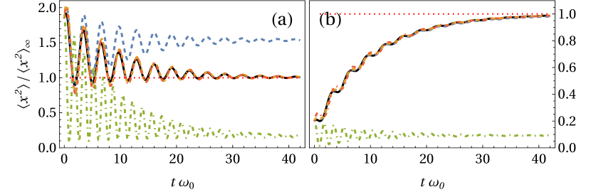
Figure 1: Dynamics of a damped harmonic oscillator. Exact thermalising dynamics of the position variance $\textstyle{\langle\boldsymbol{x}^{2}(t)\rangle}$ relative to $\langle\boldsymbol{x}^{2}\rangle_{\infty}$, for an oscillator with Hamiltonian $\textstyle{\boldsymbol{H}_{S}=\boldsymbol{H}_{S}^{(0)}+\frac{1}{2}\Delta\omega^{2}\,\boldsymbol{x}^{2}}$ (solid black) at an intermediate coupling of $\lambda=0.1\,\omega_{0}$. The Redfield equation (14) derived from this Hamiltonian (dashed blue) is accurate in the classical regime, as shown in panel (b), but breaks down at moderate and low temperatures (see (a)). Further performing the secular approximation yields even worse results (dot-dashed green). Specifically, the resulting GKLS equation forces the system into a thermal state with respect to $\textstyle{\boldsymbol{H}_{S}=\boldsymbol{H}_{S}^{(0)}+\frac{1}{2}\Delta\omega^{2}\,\boldsymbol{x}^{2}}$, which is incompatible with the correct high-temperature limit from Eq. (16). On the contrary, a Redfield equation derived from $\textstyle{\boldsymbol{H}_{S}=\boldsymbol{H}_{S}^{(0)}}$, where the counter term is removed by an adding the reorganisation energy, yields excellent results provided that all Lamb-shift terms are suppressed (dashed yellow). The secular version of this modified equation also tracks the dynamics very reliably (dot-dashed orange). Both of these equations succeed in bringing the system close to the correct mean-force Gibbs state (red dotted line) over a very broad temperature range. The parameters are $\omega_{0}=1,\lambda=0.1$ and $\Lambda=100$. Hence, $\Delta\omega^{2}=10$. Recall that we work in units of $\hbar=k=1$ . In panel (a) $T=1$ and in (b) $T=10$.

Importantly, Born–Markov master equations are often used in the context of quantum optics Carmichael (2009), thus modelling coupling to the electromagnetic field. In this case, the microscopic Hamiltonian must explicitly include a counter term compensating for any potential renormalisation Caldeira and Leggett (1983). As already advanced, $\boldsymbol{H}_{S}=\boldsymbol{H}_{S}^{(0)}+\frac{1}{2}\Delta\omega^{2}\,\boldsymbol{x}^{2}$ would then play the role of the system Hamiltonian. Strictly speaking, it this $\boldsymbol{H}_{S}$—counter term included—which must be used when deriving the Redfield equation. And, in principle, we should keep all the resulting Lamb-shift terms. In practice, however, the Hamiltonian $\boldsymbol{H}_{S}^{(0)}$ is almost universally used, while all Lamb-shift terms are removed from the master equation. Doing so, one obtains $\boldsymbol{\varrho}_{S}(t\rightarrow\infty)=\boldsymbol{\pi}_{S}$ which is the correct classical limit and, more generally, a good approximation to $\boldsymbol{\tau}_{S}$. That is, the common practice is nothing but the artefact described above; namely, the physical Hamiltonian $\boldsymbol{H}_{S}$ is being supplemented by the reorganisation energy—which cancels the counter term—while the Lamb shift is eliminated.

In fact, the idea of building the correct long-time limit into the weak-coupling master equation had been considered previously Winczewski and Alicki (2021); Łobejko et al. (2022); Timofeev and Trushechkin (2022); Becker et al. (2022). Namely, the fitness of a Redfield equation constructed from approximations to the ‘mean-force Hamiltonian’—which satisfies $\boldsymbol{\tau}_{MF}=e^{-\beta\,\boldsymbol{H}_{MF}}/\operatorname{tr}_{S}{e^{-\beta\,\boldsymbol{H}_{MF}}}$—was numerically studied, showing some improvement at long times Timofeev and Trushechkin (2022). The reason for this success can be elegantly explained by considering the Hamiltonian renormalisation procedure that would bring the interaction-picture cumulant equation into a dissipative-only form Łobejko et al. (2022); Winczewski and Alicki (2021). Similarly, using a Redfield equation modified to steer the system towards the mean-force Gibbs state was shown to outperform conventional weak-coupling equations at long times, and even to improve the accuracy of the transient dynamics of a damped harmonic oscillator Becker et al. (2022).

IV Exact dynamics

Before we turn to discussing the results, let us briefly outline the exact solution of the problem Lampo et al. (2019) (full details are given in Appendix B). The exact Heisenberg equations of motion for the system can be compacted into the well-known quantum Langevin equation Weiss (2008)

$$\ddot{\boldsymbol{x}}(t)+\omega_{0}^{2}\,\boldsymbol{x}(t)-\int_{0}^{t}d\tau\,\chi(t-\tau)\,\boldsymbol{x}(\tau)=\boldsymbol{F}(t),$$ (17)

where $\chi(t)$ is the ‘dissipation kernel’

$$\chi(t)=\sum\nolimits_{\mu}\frac{g_{\mu}^{2}}{m_{\mu}\,\omega_{\mu}}\,\sin{(\omega_{\mu}\,t)}=\frac{2}{\pi}\int_{0}^{\infty}J(\omega)\sin{(\omega t)}\,d\omega,$$

and $\boldsymbol{F}(t)$ is a quantum stochastic force, which encodes the initial conditions of the bath. It takes the form

$$\boldsymbol{F}(t)=-\sum_{\mu}g_{\mu}\left(\boldsymbol{x}_{\mu}(0)\cos{(\omega_{\mu}t)}+\frac{\boldsymbol{p}_{\mu}(0)}{m_{\mu}\omega_{\mu}}\sin{(\omega_{\mu}t)}\right).$$

Introducing the compact notation $\boldsymbol{\mathsf{Z}}=(\boldsymbol{x},\boldsymbol{p})^{\mathsf{T}}$ allows to write the exact solution of Eq. (17) as

$$\boldsymbol{\mathsf{Z}}(t)=\mathsf{G}(t)\,\boldsymbol{\mathsf{Z}}(0)+\int_{0}^{t}\mathsf{G}(t-t^{\prime})\,\boldsymbol{\mathsf{F}}(t^{\prime})\,dt^{\prime},$$ (18a)

where the entries of $$\mathsf{G}(t)$$ are

$$[\mathsf{G}(t)]_{11} =[\mathsf{G}(t)]_{22}=\pazocal{L}_{t}^{-1}\left[\frac{s}{s^{2}+\omega_{0}^{2}-\widehat{\chi}(s)}\right],$$ (18b)

$$[\mathsf{G}(t)]_{12} =\pazocal{L}_{t}^{-1}\left[\frac{1}{s^{2}+\omega_{0}^{2}-\widehat{\chi}(s)}\right]=g(t),$$ (18c)

$$[\mathsf{G}(t)]_{21} =\pazocal{L}_{t}^{-1}\left[\frac{\widehat{\chi}(s)-\omega_{0}^{2}}{s^{2}+\omega_{0}^{2}-\widehat{\chi}(s)}\right],$$ (18d)

and $\boldsymbol{\mathsf{F}}$ is defined in Appendix B. Here, $\widehat{f}(s)\mathrel{\mathop{\mathchar 58\relax}}=\int_{0}^{\infty}dt\,e^{-s\,t}\,f(t)$ stands for Laplace transform, while we denote the inverse transform by $\pazocal{L}^{-1}_{t}[\,g\,]$. For our spectral density, $\widehat{\chi}(s)$ is

$$\widehat{\chi}(s)=\frac{\lambda\Lambda^{2}}{s+\Lambda}.$$ (19)

With this, we calculate the time-evolution of the second-order moments (cf. Appendix B), which can be grouped into the covariance matrix

$$\mathsf{\Sigma}(t)=\textrm{Re}\,\langle\boldsymbol{\mathsf{Z}}(t)\,\boldsymbol{\mathsf{Z}}(t)^{\mathsf{T}}\rangle-\langle\boldsymbol{\mathsf{Z}}(t)\rangle\langle\boldsymbol{\mathsf{Z}}(t)^{\mathsf{T}}\rangle.$$ (20)

Specifically, in the long-time limit we have

$$\langle\boldsymbol{x}^{2}\rangle_{\infty}=\frac{1}{2}\int_{0}^{\infty}|\widehat{g}(i\omega)|^{2}\,\nu(\omega)\,d\omega,$$ (21a)

$$\langle\boldsymbol{p}^{2}\rangle_{\infty}=\frac{1}{2}\int_{0}^{\infty}\omega^{2}\,|\widehat{g}(i\omega)|^{2}\,\nu(\omega)\,d\omega,$$ (21b)

$$\langle\{\boldsymbol{x},\,\boldsymbol{p}\}\rangle_{\infty}=0,$$ (21c)

where we have introduced the notation

$$\nu(\omega)=\frac{2}{\pi}\,J(\omega)\,\coth{\frac{\omega}{2T}}.$$ (22)

Eqs. (21) thus yield the exact mean-force Gibbs state. More generally, Eqs. (18) and (21) above give the exact dynamics and steady state of any arbitrary linear network of harmonic oscillators, once decoupled into normal modes Martinez and Paz (2013); Freitas and Paz (2014).

V Results and discussion

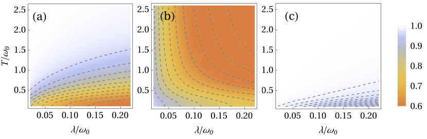
Figure 2: Benchmarking the steady state of the master equations. Uhlmann fidelity between the exact steady state $\boldsymbol{\tau}_{MF}$ and the asymptotic state resulting from different master equations, for varying temperature and system–bath coupling. Just like in Fig. 1 the microscopic model includes an explicit counter term. In (a) the resulting full Redfield equation—Lamb shift included—is benchmarked against the mean-force Gibbs state. As we see, the agreement is good as long as the temperature is not too low, or the coupling too strong. In (b) we performed the secular approximation, which yields $\boldsymbol{\pi}_{S}$ asymptotically. This is a very bad approximation to $\boldsymbol{\tau}_{MF}$ due to the large reorganisation energy in our example. Finally, in (c) we cancel the counter term and vanish the Lamb shift. The resulting steady state is the high-temperature limit from Eq. (16), which turns out to be an excellent approximation to the mean-force Gibbs state, other than at very low temperatures.

V.1 Dynamics

Let us start by looking at the transient dynamics of our model. In particular, we shall assume that the physical Hamiltonian has a built-in counter term, i.e.,

$$\boldsymbol{H}_{S}=\boldsymbol{H}_{S}^{(0)}+\frac{1}{2}\Delta\omega^{2}\,\boldsymbol{x}^{2},$$

and will focus on the evolution of the position variance $\langle\boldsymbol{x}^{2}(t)\rangle$. Its exact dynamics, as per Eq. (18), is plotted on solid black in Fig. 1. We also depict the evolution according to the Redfield equation (14) derived from the above Hamiltonian (dashed blue). As already advanced, at high temperatures the agreement is good (see Fig. 1(b)). In contrast, at low and even moderate temperatures—i.e., so that $T\lesssim\omega_{0}$—there may be a significant error (cf. Fig. 1(a)). We note however, that this deviation might be partly attributed to the rather large coupling strength of $\lambda=0.1\,\omega_{0}$. If the secular approximation is applied on such Redfield equation, the resulting dynamics (depicted in dot-dashed green) deviates from the exact one even further—neither the frequency of the oscillations nor the stationary value are captured correctly, regardless of temperature. Indeed, we know that the stationary state of Eq. (15) is always thermal with respect to the Hamiltonian; in our case, $\boldsymbol{H}_{S}=\boldsymbol{H}_{S}^{(0)}+\frac{1}{2}\Delta\omega^{2}\,\boldsymbol{x}^{2}$. The much narrower position distribution predicted by the secular equation in the steady state is thus explained by our choice of parameters, for which $\Delta\omega^{2}/\omega_{0}^{2}=10$.

In contrast, if we proceed as discussed in Sec. III.4, i.e., by cancelling the counter term with the reorganisation energy—so that $\boldsymbol{H}_{S}=\boldsymbol{H}_{S}^{(0)}$—and set $S(\omega)=0$ in Eq. (14), the resulting Redfield equation showcases an excellent agreement with the exact solution, especially at $t\gg t_{D}$ (see dashed yellow curve). Subsequently removing all non-secular terms gives

$$\frac{d\boldsymbol{\varrho}_{S}}{dt}=-i[\boldsymbol{H}_{S}^{(0)},\,\boldsymbol{\varrho}_{S}]\\ +\sum\nolimits_{\omega=\pm\omega_{0}}\gamma(\omega)\,\left(\boldsymbol{A}_{\omega}\,\boldsymbol{\varrho}_{S}\,\boldsymbol{A}_{\omega}^{\dagger}-\frac{1}{2}\,\{\boldsymbol{A}_{\omega}^{\dagger}\,\boldsymbol{A}_{\omega},\,\boldsymbol{\varrho}_{S}\}\right),$$

which is also accurate as long as the secular approximation applies. For our model, this is always the case provided that $\lambda^{2}\ll\omega_{0}^{2}+\Delta\omega^{2}$.

We also note how the Redfield equation modified according to the ‘conventional wisdom’ seems to track the dynamics very accurately at intermediate times $t\gtrsim t_{D}$. In particular, the frequency of the transient oscillations is well reproduced. This is not model-specific, but can be expected to hold generally at large-enough temperatures and in the adiabatic limit. To see this, let us consider a regime in which the full Redfield equation—counter term and Lamb shift included—yields a good approximation to the exact dynamics and steady state, e.g. that of Fig. 1(b). If the adiabatic limit is taken, the Hamiltonian correction term $\Delta\boldsymbol{H}$ cancels out with the counter term (cf. Sec. III.2) so that the oscillatory part of the dissipative dynamics, encapsulated in the commutator term of the master equation, is effectively dictated by the bare Hamiltonian $\boldsymbol{H}_{S}^{(0)}$. More generally, these oscillations are governed by $\boldsymbol{H}_{S}-Q\,\boldsymbol{S}^{2}$.

One can thus expect the common practice to yield the correct steady state in the classical regime. This is completely general. If one further works in the adiabatic limit, the transient is also qualitatively captured. In the particular case of a damped harmonic oscillator—and thus, also any arbitrary linear open network—the correct long-time limit and transient oscillatory dynamics are recovered not only in the classical regime, but also down to intermediate and low temperatures.

V.2 Steady state

So far, we have illustrated that the common practice within weak-coupling master equations does indeed work at long times. We shall now try to develop an intuition as to why it works. To that end, let us compute the Uhlmann fidelity between the exact mean-force Gibbs state from Eqs. (21) and the steady state of the weak-coupling master equations discussed above. The fidelity between undisplaced single-mode Gaussian states with covariance matrices $\mathsf{\Sigma}_{1}$ and $\mathsf{\Sigma}_{2}$ can be readily calculated using the formula Scutaru (1998)

$$\mathbb{F}(\mathsf{\Sigma}_{1},\mathsf{\Sigma}_{2})=2\left(\sqrt{\varkappa+1}-\sqrt{\Upsilon}\right)^{-1},$$

where $\varkappa=4\det{\left(\Sigma_{1}+\Sigma_{2}\right)}$ and $\Upsilon=(4\det{\Sigma_{1}}-1)(4\det{\Sigma_{2}}-1)$.

As we can see in Fig. 2(a) the Redfield equation derived from $\boldsymbol{H}_{S}=\boldsymbol{H}_{S}^{(0)}+\frac{1}{2}\Delta\omega^{2}\,\boldsymbol{x}^{2}$ gives a good approximation to the mean-force Gibbs state at high-enough temperature and weak-enough coupling $\lambda$. The secular version of such Redfield equation, however, fails miserably, other than at vanishing coupling strengths (cf. Fig. 2(b)). Crucially, as shown in Fig. 2(c), the long-time limit of the Redfield equation missing both counter term and Lamb-shift contributions provides a very good approximation to $\boldsymbol{\tau}_{MF}$ almost everywhere in parameter space. Put differently, the high-temperature formula (16) is remarkably accurate even at low temperatures.

Our observation that the mean-force Gibbs state can be approximated by the ‘semi-classical’ state $\boldsymbol{\tau}_{S}$ in (16) over a broad range of parameters is of independent interest. Indeed, expressions of the mean-force Gibbs state are only known in the weak and ultra-strong coupling limits Trushechkin et al. (2022); Łobejko et al. (2022); Cresser and Anders (2021), while intermediate couplings may be dealt-with numerically Chiu et al. (2022). Although our observations are model-specific, the same had been noted for the spin–boson model in Ref. Timofeev and Trushechkin (2022), which raises hopes for a broader applicability.

VI Conclusion

We have used a dissipative harmonic oscillator to investigate how do weak-coupling quantum master equations capture the potential renormalisation of open quantum systems. Importantly, such renormalisation is, in general, not negligible with respect to the typical energy scale of the system. We have shown how the Lamb-shift terms of the Redfield equation for our model give rise to a Hamiltonian correction which, in the adiabatic limit, closely approximates the potential renormalisation. We have also illustrated how the stationary state of this equation agrees with the exact mean-force Gibbs state at high temperatures. Such agreement, however, breaks down if the Lamb-shift terms are vanished (without making any other changes). Hence, one may not generally expect the Lamb-shift terms to have a negligible effect.

Strikingly, the standard modus operandi when it comes to weakly-coupled open quantum systems, consisting in ignoring any counter terms and removing all Lamb-shift contributions to the master equation, does achieve excellent results. We have shown that this procedure is justified not because either the renormalisation nor the Lamb shift are small, but because the combined effect of these two manipulations drives the master equation towards the correct asymptotic limit. Hence, the resulting steady state turn out much more accurate. For any open network of linearly coupled harmonic oscillators, this holds beyond the classical limit—at intermediate and even low temperatures. Importantly, this artefact also succeeds at capturing the frequency of the oscillatory transient dynamics provided that one works in the adiabatic limit. Beyond linear open networks, all the above is expected to hold at high-enough temperatures.

Two questions remain open. Firstly, to which extent does the classical mean-force Gibbs state stay close to the exact $\boldsymbol{\tau}_{MF}$ away from the classical limit? It is also important to understand whether the transient predicted by the conventional procedure remains accurate for other models at lower temperatures. These points certainly deserve further investigation.

Appendix A Redfield and GKLS equations

While we will not elaborate on the well-known steps leading to the Redfield equation (see, e.g., Ref. Gaspard and Nagaoka (1999) for a concise and rigorous derivation), we shall provide the explicit equations for the dynamics of the covariances of the system. The equations below have been derived taking $\boldsymbol{H}_{S}=\boldsymbol{H}_{S}^{(0)}$ and inserting the Redfield equation (14a) into $\frac{d}{dt}\langle\boldsymbol{O}\rangle=\operatorname{tr}_{S}(\boldsymbol{O}\,\frac{d}{dt}\boldsymbol{\varrho}_{S})$. We thus have

$$\frac{d}{dt}\langle\boldsymbol{x}\rangle =\langle\boldsymbol{p}\rangle$$

$$\frac{d}{dt}\langle\boldsymbol{p}\rangle =-(\omega_{0}^{2}-\Sigma^{\prime})\,\langle\boldsymbol{x}\rangle+\frac{\Delta}{2\omega_{0}}\,\langle\boldsymbol{p}\rangle$$

for the first-order moments and

$$\frac{d}{dt}\langle\boldsymbol{x}^{2}\rangle =\langle\{\boldsymbol{x},\boldsymbol{p}\}\rangle$$

$$\frac{d}{dt}\langle\boldsymbol{p}^{2}\rangle =\frac{\Delta}{\omega}\,\langle\boldsymbol{p}^{2}\rangle-(\omega_{0}^{2}-\Sigma^{\prime})\,\langle\{\boldsymbol{x},\boldsymbol{p}\}\rangle-\frac{\Sigma}{2}$$

$$\frac{d}{dt}\langle\{\boldsymbol{x},\boldsymbol{p}\}\rangle =-2(\omega_{0}^{2}-\Sigma^{\prime})\,\langle\boldsymbol{x}^{2}\rangle+2\,\langle\boldsymbol{p}^{2}\rangle+\frac{\Delta}{2\omega_{0}}\,\langle\{\boldsymbol{x},\boldsymbol{p}\}\rangle-\frac{\Delta^{\prime}}{\omega_{0}}$$

for the second-order moments.

Using instead the secular GKLS equation (15) gives

$$\frac{d}{dt}\langle\boldsymbol{x}\rangle =\frac{\Delta}{4\omega_{0}}\langle\boldsymbol{x}\rangle+\frac{1}{\omega_{0}^{2}}\,\left(\omega_{0}^{2}-\frac{\Sigma^{\prime}}{2}\right)\,\langle\boldsymbol{p}\rangle$$

$$\frac{d}{dt}\langle\boldsymbol{p}\rangle =-\left(\omega_{0}^{2}-\frac{\Sigma^{\prime}}{2}\right)\,\langle\boldsymbol{x}\rangle+\frac{\Delta}{4\omega_{0}}\,\langle\boldsymbol{p}\rangle$$

$$\frac{d}{dt}\langle\boldsymbol{x}^{2}\rangle =\frac{\Delta}{2\omega_{0}}\,\langle\boldsymbol{x}^{2}\rangle+\frac{1}{\omega_{0}^{2}}\,\left(\omega_{0}^{2}-\frac{\Sigma^{\prime}}{2}\right)\,\langle\{\boldsymbol{x},\boldsymbol{p}\}\rangle-\frac{\Sigma}{4\omega_{0}^{2}}$$

$$\frac{d}{dt}\langle\boldsymbol{p}^{2}\rangle =\frac{\Delta}{2\omega_{0}}\,\langle\boldsymbol{p}^{2}\rangle-\left(\omega_{0}^{2}-\frac{\Sigma^{\prime}}{2}\right)\,\langle\{\boldsymbol{x},\boldsymbol{p}\}\rangle-\frac{\Sigma}{4}$$

$$\frac{d}{dt}\langle\{\boldsymbol{x},\boldsymbol{p}\}\rangle =-(2\omega_{0}^{2}-\Sigma^{\prime})\,\langle\boldsymbol{x}^{2}\rangle+\frac{2}{\omega_{0}^{2}}\,\left(\omega_{0}^{2}-\frac{\Sigma^{\prime}}{2}\right)\,\langle\boldsymbol{p}^{2}\rangle$$

$$\qquad\qquad\qquad\qquad\qquad\qquad\quad+\frac{\Delta}{2\omega_{0}}\,\langle\{\boldsymbol{x},\boldsymbol{p}\}\rangle.$$

Appendix B Detailed solution of the exact dynamics

The Heisenberg equations of motion from the Hamiltonian $\boldsymbol{H}_{S}+\boldsymbol{V}+\boldsymbol{H}_{B}$ defined in Eqs. (2) and (3) are

$$\dot{\boldsymbol{x}} =\boldsymbol{p},$$

$$\dot{\boldsymbol{p}} =-\omega_{0}^{2}\,\boldsymbol{x}-\sum\nolimits_{\mu}g_{\mu}\,\boldsymbol{x}_{\mu},$$

$$\dot{\boldsymbol{x}}_{\mu} =\boldsymbol{p}_{\mu}/m_{\mu},$$

$$\dot{\boldsymbol{p}}_{\mu} =-m_{\mu}\omega_{\mu}^{2}\,\boldsymbol{x}_{\mu}-g_{\mu}\,\boldsymbol{x}.$$

In order to simplify notation we define $\boldsymbol{\mathsf{Z}}_{\mu}=(\boldsymbol{x}_{\mu},\boldsymbol{p}_{\mu})^{\mathsf{T}}$ and $\boldsymbol{\mathsf{Z}}=(\boldsymbol{x},\boldsymbol{p})^{\mathsf{T}}$. Hence, the equation of motion for the environmental degrees of freedom can be compactly expressed as

$$\dot{\boldsymbol{\mathsf{Z}}}_{\mu}(t)+\mathsf{\Omega}_{\mu}\boldsymbol{\mathsf{Z}}_{\mu}(t)=\mathsf{C}_{\mu}\boldsymbol{\mathsf{Z}}(t),$$

with

$$\mathsf{\Omega}_{\mu} =\begin{pmatrix}0&-m_{\mu}^{-1}\\ m_{\mu}\omega_{\mu}^{2}&0\end{pmatrix}$$

$$\mathsf{C}_{\mu} =\begin{pmatrix}0&0\\ -g_{\mu}&0\end{pmatrix}.$$

Here $\boldsymbol{\mathsf{Z}}(t)$ acts as a source term in the equations for $\boldsymbol{\mathsf{Z}}_{\mu}(t)$. Taking the Laplace transform of Eq. (23) we obtain

$$s\,\widehat{{\boldsymbol{\mathsf{Z}}}}_{\mu}(s)-\boldsymbol{\mathsf{Z}}_{\mu}(0)+\mathsf{\Omega}_{\mu}\widehat{{\boldsymbol{\mathsf{Z}}}}_{\mu}(s)=\mathsf{C}_{\mu}\widehat{{\boldsymbol{\mathsf{Z}}}}(s),$$

which can be recast as

$$\widehat{{\boldsymbol{\mathsf{Z}}}}_{\mu}(s)=\left(s\,\mathbbm{1}_{2}+\mathsf{\Omega}_{\mu}\right)^{-1}\left[\mathsf{C}_{\mu}\widehat{{\boldsymbol{\mathsf{Z}}}}(s)+\boldsymbol{\mathsf{Z}}_{\mu}(0)\right],$$

where $\mathbbm{1}_{2}$ is the $2\times 2$ identity matrix. Taking now the inverse Laplace transform we get

$$\boldsymbol{\mathsf{Z}}_{\mu}(t)=\mathsf{G}_{\mu}(t)\,\boldsymbol{\mathsf{Z}}_{\mu}(0)+\int_{0}^{t}dt^{\prime}\,\mathsf{G}_{\mu}(t-t^{\prime})\,\mathsf{C}_{\mu}\,\boldsymbol{\mathsf{Z}}(t^{\prime}).$$

Here, the elements of $\mathsf{G}_{\mu}(t)$ are

$$\mathsf{G}_{\mu}(t)=\begin{pmatrix}\cos{(\omega_{\mu}t)}&\frac{\sin{(\omega_{\mu}t)}}{m_{\mu}\,\omega_{\mu}}\\ -m_{\mu}\omega_{\mu}\sin{(\omega_{\mu}t)}&\cos{(\omega_{\mu}t)}\end{pmatrix}.$$

Using this, we can now express the equations of motion of the degrees of freedom of the system as

$$\dot{\boldsymbol{\mathsf{Z}}}(t)+\mathsf{\Omega}\,\boldsymbol{\mathsf{Z}}(t)-\int_{0}^{t}dt^{\prime}\,\mathsf{\Chi}(t-t^{\prime})\,\boldsymbol{\mathsf{Z}}(t^{\prime})=\boldsymbol{\mathsf{F}}(t),$$ (23)

with

$$\mathsf{\Omega} =\begin{pmatrix}0&-1\\ \omega_{0}^{2}&0\end{pmatrix}$$

$$\mathsf{\Chi}(t) =\begin{pmatrix}0&0\\ \chi(t)&0\end{pmatrix},$$

where the noise term is $\boldsymbol{\mathsf{F}}(t)=\sum_{\mu}\mathsf{C}_{\mu}\,\mathsf{G}_{\mu}(t)\,\boldsymbol{\mathsf{Z}}_{\mu}(0)$. Taking again the Laplace transform of (23) we obtain

$$s\,\widehat{{\boldsymbol{\mathsf{Z}}}}(s)-\boldsymbol{\mathsf{Z}}(0)+\mathsf{\Omega}\,\widehat{{\boldsymbol{\mathsf{Z}}}}(s)-\widehat{\mathsf{\Chi}}(s)\,\widehat{{\boldsymbol{\mathsf{Z}}}}(s)=\widehat{\boldsymbol{\mathsf{F}}}(s),$$

which can be recast as

$$\widehat{{\boldsymbol{\mathsf{Z}}}}(s)=\left(s\,\mathbbm{1}_{2}+\mathsf{\Omega}-\widehat{\mathsf{\Chi}}(s)\right)^{-1}\left(\widehat{\boldsymbol{\mathsf{F}}}(s)+\boldsymbol{\mathsf{Z}}(0)\right).$$

Transforming this back into the time domain takes us to Eqs. (18) from the main text. In turn, these are all we need to calculate the correlation functions of our system.

In particular, the covariance matrix (19) evolves as

$$\mathsf{\Sigma}(t)=\mathsf{G}(t)\,\mathsf{\Sigma}(0)\,\mathsf{G}(t)^{\mathsf{T}}+\mathsf{G}(t)\,\textrm{Re}\,\langle\boldsymbol{\mathsf{Z}}(0)\boldsymbol{\mathsf{B}}(t)^{\mathsf{T}}\rangle\\ +\textrm{Re}\,\langle\boldsymbol{\mathsf{B}}(t)\boldsymbol{\mathsf{Z}}(0)^{\mathsf{T}}\rangle\,\mathsf{G}(t)^{\mathsf{T}}+\textrm{Re}\,\langle\boldsymbol{\mathsf{B}}(t)\boldsymbol{\mathsf{B}}(t)^{\mathsf{T}}\rangle,$$ (24)

with $\boldsymbol{\mathsf{B}}(t)=\int_{0}^{\infty}\,\mathsf{G}(t-t^{\prime})\,\boldsymbol{\mathsf{F}}(t^{\prime})\,dt^{\prime}$. The second and third term are propagations of the initial probe–sample correlations and therefore vanish for our factorised preparation. In turn, the first term vanishes asymptotically, so that it must be considered when studying the dynamics of the system. We now turn our attention to the more complicated fourth term, which we dub ‘memory integral’ term. Explicitly, this is given by

$$\mathsf{\Sigma}_{\text{mi}}(t)=\textrm{Re}\,\langle\boldsymbol{\mathsf{B}}(t)\boldsymbol{\mathsf{B}}(t)^{\mathsf{T}}\rangle=\int_{0}^{t}dt_{1}\int_{0}^{t}dt_{2}\,\mathsf{G}(t-t_{1})\sum\nolimits_{\mu\nu}\mathsf{C}_{\mu}\mathsf{G}_{\mu}(t_{1})\,\textrm{Re}\,\langle\boldsymbol{\mathsf{Z}}_{\mu}(0)\boldsymbol{\mathsf{Z}}_{\nu}(0)^{\mathsf{T}}\rangle\mathsf{G}_{\nu}(t_{2})^{\mathsf{T}}\mathsf{C}^{\mathsf{T}}_{\nu}\mathsf{G}(t-t_{2})^{\mathsf{T}}\,.$$ (25)

Since the bath is in thermal equilibrium at temperature $T$

$$\textrm{Re}\,\langle\boldsymbol{\mathsf{Z}}_{\mu}(0)\,\boldsymbol{\mathsf{Z}}_{\nu}(0)^{\mathsf{T}}\rangle\\ =\delta_{\mu\nu}\begin{pmatrix}\frac{1}{2\,m_{\mu}\omega_{\mu}}\coth\frac{\omega_{\mu}}{2T}&0\\ 0&\frac{m_{\mu}\omega_{\mu}}{2}\coth\frac{\omega_{\mu}}{2T}\end{pmatrix},$$

where $\delta_{\mu\nu}$ is a Kronecker delta. Eq. (25) thus simplifies to

$$\mathsf{\Sigma}^{\text{mi}}(t)=\frac{1}{2}\,\int_{0}^{t}dt_{1}\int_{0}^{t}dt_{2}\,\mathsf{G}(t-t_{1})\begin{pmatrix}0&0\\ 0&\mu(t_{1}-t_{2})\end{pmatrix}\mathsf{G}(t-t_{2})^{\mathsf{T}},$$ (26)

with the ‘noise kernel’ $\mu(t)$ given by

$$\mu(t)=\sum\nolimits_{\mu}\frac{g_{\mu}^{2}}{m_{\mu}\omega_{\mu}}\,\cos{\omega_{\mu}t}\,\coth{\frac{\omega_{\mu}}{2T}}\\ =\frac{2}{\pi}\,\int_{0}^{\infty}d\omega\,J(\omega)\,\cos{\omega t}\,\coth{\frac{\omega}{2T}}.$$

Finally, Eq. (26) reduces to the following expressions for the memory-integral contribution to the elements of $\mathsf{\Sigma}(t)$:

$$[\mathsf{\Sigma}^{\text{mi}}(t)]_{11} =\frac{1}{2}\int_{0}^{t}dt_{1}\int_{0}^{t}dt_{2}~{}g(t-t_{1})\,\mu(t_{1}-t_{2})\,g(t-t_{2}),$$

$$[\mathsf{\Sigma}^{\text{mi}}(t)]_{22} =\frac{1}{2}\int_{0}^{t}dt_{1}\int_{0}^{t}dt_{2}~{}\partial_{t}\,g(t-t_{1})\,\mu(t_{1}-t_{2})\,\partial_{t}g(t-t_{2}),$$

$$[\mathsf{\Sigma}^{\text{mi}}(t)]_{12} =\frac{1}{2}\int_{0}^{t}dt_{1}\int_{0}^{t}dt_{2}~{}g(t-t_{1})\,\mu(t_{1}-t_{2})\,\partial_{t}g(t-t_{2}).$$

Note that since the inverse Laplace transform is given by the Bromwich integral, the diagonal elements of $\mathsf{G}(t)$ can be cast as $[\mathsf{G}(t)]_{11}=[\mathsf{G}(t)]_{22}=\partial_{t}g(t)$.

In order to study the steady state, it is convenient to write the covariances as

$$[\mathsf{\Sigma}^{\text{mi}}(t)]_{11}=\langle\boldsymbol{x}^{2}(t)\rangle^{\text{mi}}=\int_{0}^{\infty}d\omega\,\nu(\omega)\,\varsigma_{xx}(t,\omega)$$

where $\nu(\omega)$ was defined in Eq. (22) and thus,

$$\varsigma_{xx}(t,\omega) =\frac{1}{2}\int_{0}^{t}dt_{1}\int_{0}^{t}dt_{2}~{}g(t-t_{1})\,\cos{[\omega(t_{1}-t_{2})]}\,g(t-t_{2})$$

$$=\frac{1}{4}\int_{0}^{t}du_{1}~{}g(u_{1})\,e^{-i\,\omega\,u_{1}}\int_{0}^{t}du_{2}~{}g(u_{2})\,e^{i\,\omega\,u_{2}}+\text{c.c.}.$$

Here, we have used Euler’s formula, $\cos{x}=\frac{1}{2}(e^{i\,x}+e^{-i\,x})$, and introduced the variables $u_{j}=t-t_{j}$. Asymptotically, this gives

$$\lim\nolimits_{t\rightarrow\infty}\,\varsigma_{xx}(t,\omega) =\frac{1}{2}~{}\widehat{g}(-i\,\omega)~{}\widehat{g}(i\,\omega),$$

which brings us to Eq. (21a) in the main text; namely,

$$\langle\boldsymbol{x}^{2}\rangle_{\infty}=\frac{1}{2}\int_{0}^{\infty}|\widehat{g}(i\omega)|^{2}\,\nu(\omega)\,d\omega.$$

Note that we have set the first term in Eq. (24) to zero (i.e., $\langle\boldsymbol{x}^{2}\rangle^{\text{mi}}_{\infty}=\langle\boldsymbol{x}^{2}\rangle_{\infty}$), since it vanishes in steady state.

Now, using the fact that $g(0)=[\mathsf{G}(0)]_{12}=0$, we see that $\widehat{\partial_{t}\,g}(s)=s\,\widehat{g}(s)$, which gives a vanishing asymptotic position–momentum covariance $\langle\{\boldsymbol{x},\boldsymbol{p}\}\rangle_{\infty}=0$, since

$$\lim\nolimits_{t\rightarrow\infty}\varsigma_{xp}(t,\omega)=\frac{1}{4}\big{[}i\,\omega\,|\widehat{g}(i\,\omega)|^{2}-i\,\omega\,|\widehat{g}(i\,\omega)|^{2}\big{]}=0.$$

Finally, for momentum variance we have

$$\lim\nolimits_{t\rightarrow\infty}\varsigma_{pp}(t,\omega)=\frac{1}{2}\,\omega^{2}\,|\widehat{g}(i\,\omega)|^{2},$$

so that we recover Eq. (21b).

References

- Alicki and Kosloff (2018) R. Alicki and R. Kosloff, Introduction to quantum thermodynamics: History and prospects, in Thermodynamics in the Quantum Regime: Fundamental Aspects and New Directions, edited by F. Binder, L. A. Correa, C. Gogolin, J. Anders, and G. Adesso (Springer International Publishing, Cham, 2018) pp. 1–33.
- Alicki (1979) R. Alicki, The quantum open system as a model of the heat engine, J. Phys. A. 12, L103 (1979).
- Geva and Kosloff (1992) E. Geva and R. Kosloff, A quantum‐mechanical heat engine operating in finite time. A model consisting of spin‐1/2 systems as the working fluid, J. Chem. Phys 96, 3054 (1992).
- Kosloff and Levy (2014) R. Kosloff and A. Levy, Quantum heat engines and refrigerators: Continuous devices, Annu. Rev. Phys. Chem. 65, 365 (2014).
- Ghosh et al. (2018) A. Ghosh, W. Niedenzu, V. Mukherjee, and G. Kurizki, Thermodynamic principles and implementations of quantum machines, in Thermodynamics in the Quantum Regime: Fundamental Aspects and New Directions, edited by F. Binder, L. A. Correa, C. Gogolin, J. Anders, and G. Adesso (Springer International Publishing, Cham, 2018) pp. 37–66.
- Zou et al. (2017) Y. Zou, Y. Jiang, Y. Mei, X. Guo, and S. Du, Quantum heat engine using electromagnetically induced transparency, Phys. Rev. Lett. 119, 050602 (2017).
- Brantut et al. (2013) J.-P. Brantut, C. Grenier, J. Meineke, D. Stadler, S. Krinner, C. Kollath, T. Esslinger, and A. Georges, A thermoelectric heat engine with ultracold atoms, Science 342, 713 (2013).
- Roßnagel et al. (2016) J. Roßnagel, S. T. Dawkins, K. N. Tolazzi, O. Abah, E. Lutz, F. Schmidt-Kaler, and K. Singer, A single-atom heat engine, Science 352, 325 (2016).
- von Lindenfels et al. (2019) D. von Lindenfels, O. Gräb, C. T. Schmiegelow, V. Kaushal, J. Schulz, M. T. Mitchison, J. Goold, F. Schmidt-Kaler, and U. G. Poschinger, Spin heat engine coupled to a harmonic-oscillator flywheel, Phys. Rev. Lett. 123, 080602 (2019).
- Thierschmann et al. (2015) H. Thierschmann, R. Sánchez, B. Sothmann, F. Arnold, C. Heyn, W. Hansen, H. Buhmann, and L. W. Molenkamp, Three-terminal energy harvester with coupled quantum dots, Nat. Nanotechnol. 10, 854 (2015).
- Klatzow et al. (2019) J. Klatzow, J. N. Becker, P. M. Ledingham, C. Weinzetl, K. T. Kaczmarek, D. J. Saunders, J. Nunn, I. A. Walmsley, R. Uzdin, and E. Poem, Experimental demonstration of quantum effects in the operation of microscopic heat engines, Phys. Rev. Lett. 122, 110601 (2019).
- Onsager (1933) L. Onsager, Theories of concentrated electrolytes. Chem. Rev. 13, 73 (1933).
- Jarzynski (2004) C. Jarzynski, Nonequilibrium work theorem for a system strongly coupled to a thermal environment, J. Stat. Mech. 2004, P09005 (2004).
- Trushechkin et al. (2022) A. S. Trushechkin, M. Merkli, J. D. Cresser, and J. Anders, Open quantum system dynamics and the mean force gibbs state, AVS Quantum Sci. 4 (2022), 10.1116/5.0073853.
- Subaş ı et al. (2012) Y. Subaş ı, C. H. Fleming, J. M. Taylor, and B. L. Hu, Equilibrium states of open quantum systems in the strong coupling regime, Phys. Rev. E 86, 061132 (2012).
- Cerisola et al. (2022) F. Cerisola, M. Berritta, S. Scali, S. A. R. Horsley, J. D. Cresser, and J. Anders, Quantum-classical correspondence in spin-boson equilibrium states at arbitrary coupling, (2022), arXiv:2204.10874 .
- Cresser and Anders (2021) J. D. Cresser and J. Anders, Weak and ultrastrong coupling limits of the quantum mean force Gibbs state, Phys. Rev. Lett. 127, 250601 (2021).
- Timofeev and Trushechkin (2022) G. M. Timofeev and A. S. Trushechkin, Hamiltonian of mean force in the weak-coupling and high-temperature approximations and refined quantum master equations, Int. J. Mod. Phys. A 37, 2243021 (2022).
- Wu et al. (2010) J. Wu, F. Liu, Y. Shen, J. Cao, and R. J. Silbey, Efficient energy transfer in light-harvesting systems, i: optimal temperature, reorganization energy and spatial–temporal correlations, New J. Phys. 12, 105012 (2010).
- Ritschel et al. (2011) G. Ritschel, J. Roden, W. T. Strunz, and A. Eisfeld, An efficient method to calculate excitation energy transfer in light-harvesting systems: application to the fenna–matthews–olson complex, New J. Phys. 13, 113034 (2011).
- Weiss (2008) U. Weiss, Quantum Dissipative Systems, 3rd ed. (WORLD SCIENTIFIC, 2008).
- Caldeira and Leggett (1983) A. O. Caldeira and A. J. Leggett, Quantum tunnelling in a dissipative system, Ann. Phys. 149, 374 (1983).
- Correa et al. (2019) L. A. Correa, B. Xu, B. Morris, and G. Adesso, Pushing the limits of the reaction-coordinate mapping, J. Chem. Phys. 151, 094107 (2019).
- Redfield (1957) A. G. Redfield, On the theory of relaxation processes, IBM J. Res. Dev. 1, 19 (1957).
- Redfield (1965) A. Redfield, The theory of relaxation processes, Adv. Magn. Opt. Reson. 1, 1 (1965).
- Cresser and Facer (2017) J. Cresser and C. Facer, Coarse-graining in the derivation of markovian master equations and its significance in quantum thermodynamics, (2017), arXiv:1710.09939 .
- Winczewski and Alicki (2021) M. Winczewski and R. Alicki, Renormalization in the theory of open quantum systems via the self-consistency condition, (2021), arXiv:2112.11962 .
- Davies (1974) E. B. Davies, Markovian master equations, Commun. Math. Phys. 39, 91 (1974).
- Gorini et al. (1976) V. Gorini, A. Kossakowski, and E. C. G. Sudarshan, Completely positive dynamical semigroups of n-level systems, J. Math. Phys. 17, 821 (1976).
- Lindblad (1976) G. Lindblad, On the generators of quantum dynamical semigroups, Commun. Math. Phys. 48, 119 (1976).
- Breuer and Petruccione (2002) H.-P. Breuer and F. Petruccione, The theory of open quantum systems (Oxford University Press, 2002).
- Cattaneo et al. (2019) M. Cattaneo, G. L. Giorgi, S. Maniscalco, and R. Zambrini, Local versus global master equation with common and separate baths: superiority of the global approach in partial secular approximation, New J. Phys. 21, 113045 (2019).
- Bateman (1954) H. Bateman, Tables of integral transforms, Vol. 1 (McGraw-Hill book company, 1954).
- Hartmann and Strunz (2020) R. Hartmann and W. T. Strunz, Environmentally induced entanglement–anomalous behavior in the adiabatic regime, Quantum 4, 347 (2020).
- Duffus et al. (2017) S. N. A. Duffus, V. M. Dwyer, and M. J. Everitt, Open quantum systems, effective hamiltonians, and device characterization, Phys. Rev. B 96, 134520 (2017).
- Ferraro et al. (2005) A. Ferraro, S. Olivares, and M. G. A. Paris, Gaussian States in Quantum Information, Napoli Series on physics and Astrophysics (Bibliopolis, 2005).
- Carmichael (2009) H. Carmichael, An open systems approach to quantum optics: lectures presented at the Université Libre de Bruxelles, October 28 to November 4, 1991, Vol. 18 (Springer Science & Business Media, 2009).
- Łobejko et al. (2022) M. Łobejko, M. Winczewski, G. Suárez, R. Alicki, and M. Horodecki, Towards reconciliation of completely positive open system dynamics with the equilibration postulate, (2022), arXiv:2204.00643 .
- Becker et al. (2022) T. Becker, A. Schnell, and J. Thingna, Canonically consistent quantum master equation, Phys. Rev. Lett. 129, 200403 (2022).
- Lampo et al. (2019) A. Lampo, M. Á. G. March, and M. Lewenstein, Quantum Brownian motion revisited: extensions and applications (Springer, 2019).
- Martinez and Paz (2013) E. A. Martinez and J. P. Paz, Dynamics and thermodynamics of linear quantum open systems, Phys. Rev. Lett. 110, 130406 (2013).
- Freitas and Paz (2014) N. Freitas and J. P. Paz, Analytic solution for heat flow through a general harmonic network, Phys. Rev. E 90, 042128 (2014).
- Scutaru (1998) H. Scutaru, Fidelity for displaced squeezed thermal states and the oscillator semigroup, J. Phys. A Math. Gen. 31, 3659 (1998).
- Chiu et al. (2022) Y.-F. Chiu, A. Strathearn, and J. Keeling, Numerical evaluation and robustness of the quantum mean-force gibbs state, Phys. Rev. A 106, 012204 (2022).
- Gaspard and Nagaoka (1999) P. Gaspard and M. Nagaoka, Slippage of initial conditions for the redfield master equation, J. Chem. Phys. 111, 5668 (1999).