$L_{2}$-small ball asymptotics
for Gaussian random functions: a survey

Abstract

This article is a survey of the results on asymptotic behavior of small ball probabilities in $L_{2}$-norm.

Dedicated to the memory of M.S. Birman and M.Z. Solomyak,

founders of St. Petersburg school of spectral theory

1 Introduction

The theory of small ball probabilities (also called small deviation probabilities) is extensively studied in recent decades (see the surveys by M.A. Lifshits [97], W.V. Li and Q.-M. Shao [93] and V.R. Fatalov [51]; for the extensive up-to-date bibliography see [99]). Given a random vector $X$ in a Banach space $\mathfrak{B}$, the relation

$$\mathbb{P}\left\{\|X\|_{\mathfrak{B}}\leq\varepsilon\right\}\sim f(\varepsilon),\qquad\varepsilon\to 0,$$ (1)

(here and later on $f(\varepsilon)\sim g(\varepsilon)$ as $\varepsilon\to 0$ means $\lim\limits_{\varepsilon\to 0}f(\varepsilon)/g(\varepsilon)=1$) is called an exact asymptotics of small deviations. Typically, this probability is exponentially small, and often a logarithmic asymptotics is studied, that is the relation

$$\log\big{(}\mathbb{P}\{\|X\|_{\mathfrak{B}}\leq\varepsilon\}\big{)}\sim f(\varepsilon),\qquad\varepsilon\to 0.$$

Theory of small deviations has numerous applications including the complexity problems [135], the quantization problem [64], [106], the calculation of the metric entropy for functional sets [97, Section 3], functional data analysis [52], nonparametric Bayesian estimation [170], machine learning [150] (more applications and references can be found in [93, Chapter 7]).

The discussed topic is almost boundless, so in this paper we focus on the most elaborated (and may be the simplest) case, where $X$ is Gaussian and the norm is Hilbertian. Let $X$ be a Gaussian random vector in the (real, separable) Hilbert space $\mathfrak{H}$ (the basic example is a Gaussian random function in $L_{2}({\cal O})$, where ${\cal O}$ is a domain in $\mathbb{R}^{d}$). We always assume that $\mathbb{E}X=0$ and denote by $\mathcal{G}_{X}$ corresponding covariance operator (it is a compact non-negative operator in $\mathfrak{H}$).

Let $(\mu_{k})$ be a non-increasing sequence of positive eigenvalues of $\mathcal{G}_{X}$, counted with their multiplicities, and denote by $(\varphi_{k})$ a complete orthonormal system of the corresponding eigenvectors. It is well known (see, e.g., [98, Chapter 2]) that if $\xi_{k}$ are i.i.d. standard normal random variables, then we have the following distributional equality

$$X\stackrel{{\scriptstyle d}}{{=}}\sum\limits_{k=1}^{\infty}\sqrt{\mu_{k}}\,\varphi_{k}\,\xi_{k},$$

which is usually called the Karhunen–Loève expansion. By the orthonormality of the system $(\varphi_{k})$ this implies

$$\|X\|_{\mathfrak{H}}^{2}\stackrel{{\scriptstyle d}}{{=}}\sum\limits_{k=1}^{\infty}\mu_{k}\xi_{k}^{2}.$$ (2)

Therefore the small ball asymptotics for $X$ in the Hilbertian case is completely determined by the eigenvalues $\mu_{k}$.

Notice that if $\sum\limits_{k=1}^{\infty}\mu_{k}<\infty$ then the series in (2) converges almost surely (a.s.), otherwise it diverges a.s. The latter is impossible for $X\in\mathfrak{H}$, so, in what follows we always assume that $\mathcal{G}_{X}$ is the trace class operator.

Remark 1.

Formula (2) shows that if the covariance operators of two Gaussian random vectors $X$ and $Y$ have equal spectra (excluding maybe zero eigenvalues), then their Hilbertian norms coincide in distribution. In this case $X$ and $Y$ are called spectrally equivalent. Trivially, such Gaussian random vectors have the same $L_{2}$-small ball asymptotics.

Concrete examples of spectrally equivalent Gaussian processes are well known, see, e.g., [47], [85, Example 4], [146], [114, Theorem 4.1], [104]. Some multivariate generalizations can be found in [44], [136], [41].

Recently A.I. Nazarov and Ya.Yu. Nikitin [124] (see also [123]) developed a general operator approach to the problem of spectral equivalence and obtained a number of new examples.

Our paper is organized as follows. In Section 2 we describe the first separated results on small ball probabilities in Hilbertian norm. In Section 3 we formulate two crucial results: the Wenbo Li comparison principle and the Dunker–Lifshits–Linde formula. These results formed the base for the systematic attack of the problem.

Further progress in the field is mainly based on the methods of spectral theory. In Section 4 we give an overview of results on exact asymptotics. These results are mostly related to the spectral theory of differential operators. Section 5 is devoted to the logarithmic asymptotics, corresponding results are related to the spectral theory of integral operators.

In Appendix we provide the history (up to our knowledge) of results on $L_{2}$-small ball asymptotics for concrete processes.

Let us introduce some notation.

For $\mathcal{O}\subset\mathbb{R}^{d}$, $\|\cdot\|_{2,\mathcal{O}}$ stands for the norm in $L_{2}(\mathcal{O})$:

$$\|X\|_{2,\mathcal{O}}^{2}=\int\limits_{\mathcal{O}}|X(x)|^{2}\,dx.$$

The Sobolev space $W_{p}^{m}[0,1]$ is the space of functions $u$ having continuous derivatives up to $(m-1)$-th order when $u^{(m-1)}$ is absolutely continuous on $[0,1]$ and $u^{(m)}\in L_{p}[0,1]$. For $p=2$, it is a Hilbert space.

A measurable function $f(x)$ is called regularly varying at infinity (see, e.g. [160, Chapter 1]), if it is of constant sign on $[A,\infty)$, for some $A>0$, and there exists $\alpha\in\mathbb{R}$ such that for arbitrary $\rho>0$ we have

$$\lim\limits_{x\to\infty}\frac{f(\rho x)}{f(x)}=\rho^{\alpha}.$$

Such $\alpha$ is called the index of the regularly varying function. Regularly varying function of index $\rho=0$ is called the slowly varying function (SVF). For instance, the functions $\log^{\sigma}(x)$, $\sigma\in\mathbb{R}$, are slowly varying at infinity.

A function $f(x)$ is called regularly varying at zero, if $f(\frac{1}{x})$ is a regularly varying at infinity. We say that a sequence $(a_{k})$ has regular behavior if $a_{k}=f(k)$, where $f(x)$ is regularly varying at infinity.

2 First works

The oldest results about $L_{2}$-small ball probabilities concern classical Gaussian processes on the interval $[0,1]$. R. Cameron and W. Martin [28] proved the relation for the Wiener process $W(t)$

$$\mathbb{P}\bigl{\{}\|W\|_{2,[0,1]}\leq\varepsilon\bigr{\}}\sim\frac{4\varepsilon}{\sqrt{\pi}}\exp\bigl{(}-\frac{1}{8}\,\varepsilon^{-2}\bigr{)},$$

while T. Anderson and D. Darling [5] established the corresponding asymptotics for the Brownian bridge $B(t)$

$$\mathbb{P}\bigl{\{}\|B\|_{2,[0,1]}\leq\varepsilon\bigr{\}}\sim\frac{\sqrt{8}}{\sqrt{\pi}}\exp\bigl{(}-\frac{1}{8}\,\varepsilon^{-2}\bigr{)}.$$ (3)

The latter formula describes the lower tails of famous Cramer–von Mises–Smirnov $\omega^{2}$-statistic.

One should notice that a minor difference (rank one process) between Wiener process and Brownian bridge influences the power term in the asymptotics but not the exponential one.

In general case the problem of $L_{2}$-small ball asymptotics was solved by G. Sytaya [166], but in an implicit way. The main ingredient was the Laplace transform and the saddle point technique. The general formulation of result by Sytaya in terms of operator theory states as follows.

Theorem 1 ([166, Theorem 1]).

As $\varepsilon\to 0$, we have

$$\mathbb{P}\Bigl{\{}\|X\|_{\mathfrak{H}}\leq\varepsilon\Bigr{\}}\sim\bigl{(}4\gamma^{2}\pi\,\mathrm{Tr}(\mathcal{G}_{X}R_{\gamma}(\mathcal{G}_{X}))^{2}\bigr{)}^{-\frac{1}{2}}\times\\ \times\exp\biggl{(}-\int\limits_{0}^{\gamma}\mathrm{Tr}(\mathcal{G}_{X}[R_{u}(\mathcal{G}_{X})-R_{\gamma}(\mathcal{G}_{X})])\,du\biggr{)}.$$ (4)

Here $\mathrm{Tr}(\mathcal{G})$ is the trace of operator $\mathcal{G}$; $R_{u}(\mathcal{G})$ is the resolvent operator defined by the formula

$$R_{u}(\mathcal{G})=(I+2u\mathcal{G})^{-1},$$

and $\gamma=\gamma(\varepsilon)$ satisfies the equation $\varepsilon^{2}=\mathrm{Tr}(\mathcal{G}_{X}R_{\gamma}(\mathcal{G}_{X}))$.

In terms of eigenvalues $\mu_{k}$ of the covariance operator $\mathcal{G}_{X}$, this result reads as follows:

Theorem 2 ([166, formula (20)]).

If $\mu_{k}>0$ and $\sum\limits_{k=1}^{\infty}\mu_{k}<\infty$, then as $\varepsilon\to 0$

$$\mathbb{P}\Bigl{\{}\sum\limits_{k=1}^{\infty}\mu_{k}\xi_{k}^{2}\leq\varepsilon^{2}\Bigr{\}}\sim\bigl{(}-2\pi\gamma^{2}h^{\prime\prime}(\gamma)\bigr{)}^{-\frac{1}{2}}\exp\bigl{(}\gamma h^{\prime}(\gamma)-h(\gamma)\bigr{)},$$ (5)

where $h(\gamma)=\frac{1}{2}\sum\limits_{k=1}^{\infty}\log(1+2\mu_{k}\gamma)$ and $\gamma$ is uniquely determined by equation $\varepsilon^{2}=h^{\prime}(\gamma)$ for $\varepsilon>0$ small enough.

As a particular case the formula (3) for the Brownian bridge was also obtained. However, these theorems are not convenient to use for concrete computations and applications. For example, finding expressions for the function $h(\gamma)$ and determining the implicit relation $\gamma=\gamma(\varepsilon)$ are the two difficulties that arise. The significant simplification was done only in 1997 by T. Dunker, W. Linde and M. Lifshits [49]. We describe it in detail in Section 3.

The results of [166] were not widely known. J. Hoffmann-Jørgensen [65] in 1976 obtained two-sided estimates for $L_{2}$-small ball probabilities. Later the result of Sytaya was rediscovered by I.A. Ibragimov [69]. Cf. also [110], [38], [108], [45], [4].

In 1984 V.M. Zolotarev [181] suggested an explicit description of the small deviations in the case $\mu_{k}=\phi(k)$ with a decreasing and logarithmically convex function $\phi$ on $[1,\infty)$. His method was based on application of the Euler-Maclaurin formula to sums in the right hand side of (5). Unfortunately, no proofs were presented in [181], and, as was shown in [49], this result is not valid without additional assumptions about the function $\phi$ (in particular, the final formula in [181, Example 2] is not correct, see the end of Section 3 below).

In 1989 A.A. Borovkov and A.A. Mogul’skii [22] investigated small deviations of several Gaussian processes in various norms. However, as noted in [97, Section 1], the result of Theorem 3 in [22] contains an algebraic error.

One of the natural extensions of the problem under consideration is to find asymptotics (1) for shifted small balls. It was shown in [166, Theorem 1] that if the shift $a$ belongs to the reproducing kernel Hilbert space (RKHS) of the Gaussian vector $X$, then

$$\mathbb{P}\{\|X-a\|_{\mathfrak{H}}\leq\varepsilon\}\sim\mathbb{P}\{\|X\|_{\mathfrak{H}}\leq\varepsilon\}\cdot\exp\bigl{(}-\bigl{\|}\mathcal{G}_{X}^{-\frac{1}{2}}a\bigr{\|}_{\mathfrak{H}}^{2}/2\bigr{)},$$ (6)

where $\|\mathcal{G}_{X}^{-\frac{1}{2}}a\|_{\mathfrak{H}}$ is in fact the norm of $a$ in RKHS of $X$. See also some relations between the probabilities of centered and shifted balls in [66] by J. Hoffmann-Jørgensen, L.A. Shepp and R.M. Dudley, [103] by W. Linde and J. Rosinski, and [46] by S. Dereich. A generalized version of equivalence (6) for Gaussian Radon measures on locally convex vector spaces was proved by Ch. Borell [21].

Formula (6) was later generalized by J. Kuelbs, W.V. Li and W. Linde [89] and W.V. Li, W. Linde [94], who handled the asymptotics of probability

$$\mathbb{P}\{\|X-f(t)a\|_{\mathfrak{H}}\leq R(t)\},\qquad t\to\infty,$$

for various combinations of $f$ and $R$, including the case $R(t)\to\infty$ as $t\to\infty$.

3 Second wave

The main difficulty in using Theorem 2 is that the explicit formulae for the eigenvalues of the covariance operators are rarely known. It was partially overcome by the celebrated Wenbo Li comparison principle.

Theorem 3 ([92, 59]).

Let $\xi_{k}$ be i.i.d. standard normal random variables, and let $(\mu_{k})$ and $(\tilde{\mu}_{k})$ be two positive non-increasing summable sequences such that $\prod\mu_{k}/\tilde{\mu}_{k}<\infty$. Then

$$\mathbb{P}\Big{\{}\sum_{k=1}^{\infty}\tilde{\mu}_{k}\xi_{k}^{2}\leq\varepsilon^{2}\Big{\}}\sim\mathbb{P}\Big{\{}\sum_{k=1}^{\infty}\mu_{k}\xi_{k}^{2}\leq\varepsilon^{2}\Big{\}}\cdot\Big{(}\prod\limits_{k=1}^{\infty}\frac{\mu_{k}}{\tilde{\mu}_{k}}\Big{)}^{\frac{1}{2}},\qquad\varepsilon\to 0.$$ (7)

So, if we know sufficiently sharp (and sufficiently simple!) asymptotic approximations $\tilde{\mu}_{k}$ for the eigenvalues $\mu_{k}$ of $\mathcal{G}_{X}$ then formula (7) provides the $L_{2}$-small ball asymptotics for $X$ up to a constant. However, to use this idea efficiently, we need explicit expressions of $L_{2}$-small ball asymptotics for “model” sequences $(\tilde{\mu}_{k})$.

The important step in the latter problem was made by M.A. Lifshits in [96] who considered the small ball problem for more general series:

$$\mathcal{S}:=\sum\limits_{k=1}^{\infty}\phi(k)Z_{k},$$ (8)

where $(\phi(k))$ is a non-increasing summable sequence of positive numbers, and $Z_{k}$ are independent copies of a positive random variable $Z$ with finite variance and absolutely continuous distribution. The main restriction imposed in [96] on the distribution function $F(\cdot)$ of $Z$ is

$$c_{1}F(\tau)\leq F(b\tau)\leq c_{2}F(\tau)$$ (9)

for some $b,c_{1},c_{2}\in(0,1)$ and for all sufficiently small $\tau$. This assumption implies a polynomial (but not necessarily regular) lower tail behavior of the distribution. For the special case $Z_{k}=\xi_{k}^{2}$ the sum in (8) corresponds to $L_{2}$-small ball probabilities (2).

Using the idea of R.A. Davis and S.I. Resnick [40], Lifshits expressed the exact small ball behavior of (8) in terms of the Laplace transform of $\cal S$. If $Z$ has finite third moment, then a quantitative estimate of the remainder term was also given.

The next important step was done by T. Dunker, M.A. Lifshits and W. Linde in [49]. The result is based on the following assumption on the sequence $(\phi(k))$:

Condition DLL. The sequence $(\phi(k))$ admits a positive, logarithmically convex, twice differentiable and integrable extension on the interval $[1,+\infty)$.

Under some additional assumptions on the distribution function $F$ authors significantly simplified the expressions from [96] for the small ball behavior of $\cal S$. By using Euler–Maclaurin’s summation formula, they succedeed to express the small ball probabilities in terms of three integrals:

$$I_{0}(\gamma): =\int\limits_{1}^{\infty}(\log f)(\gamma\phi(t))\,dt,$$

$$I_{1}(\gamma): =\int\limits_{1}^{\infty}\gamma\phi(t)(\log f)^{\prime}(\gamma\phi(t))\,dt,$$

$$I_{2}(\gamma): =\int\limits_{1}^{\infty}(\gamma\phi(t))^{2}(\log f)^{\prime\prime}(\gamma\phi(t))\,dt.$$

Here $f(\gamma)$ is the Laplace transform of $Z$,

$$f(\gamma) :=\int\limits_{0}^{\infty}\exp(-\gamma\tau)\,dF(\tau).$$

The main result (Theorem 3.1 in [49]) reads as follows:

$$\mathbb{P}\Bigl{\{}\mathcal{S}\leq r\Bigr{\}}\sim\sqrt{\frac{f(\gamma\phi(1))}{2\pi I_{2}(\gamma)}}\exp(I_{0}(\gamma)+\rho(\gamma)+\gamma r)),\qquad r\to 0,$$ (10)

where $\gamma=\gamma(r)$ is any function satisfying

$$\lim\limits_{r\to 0}\frac{I_{1}(\gamma)+\gamma r}{\sqrt{I_{2}(\gamma)}}=0,$$ (11)

and $\rho(\gamma)$ is a bounded function that represents the remainder terms in Euler–Maclaurin formula and can be written explicitly via infinite sums.

At a first glance, formula (10) and condition (11) do not seem to be more explicit than Theorem 2. Hovewer, for $Z_{k}=\xi_{k}^{2}$ (in this case $f(\gamma)=(1+2\gamma)^{-\frac{1}{2}}$) the result of [49] turned out to be much more computationally tractable and became the base for derivation of the exact asymptopics for many “model” sequences of eigenvalues $(\phi(k))$.

In particular, the following asymptotics were obtained in [49, Section 4].

1. Let $p>1$. Then, as $\varepsilon\to 0$,

   $$\mathbb{P}\Big{\{}\sum_{k=1}^{\infty}k^{-p}\xi_{k}^{2}\leq\varepsilon^{2}\Big{\}}\sim{\cal C}\cdot\varepsilon^{\gamma}\exp\left(-\ D\varepsilon^{-\frac{2}{p-1}}\right),$$ (12)

   where the constants $D$ and $\gamma$ depend on $p$ as follows:

   $$D=\frac{p-1}{2}\Big{(}\frac{\pi}{p\sin\frac{\pi}{p}}\Big{)}^{\frac{p}{p-1}},\qquad\gamma=\frac{2-p}{2(p-1)},$$

   while the constant ${\cal C}$ is given by the following expression:

   $${\cal C}=\frac{(2\pi)^{\frac{p}{4}}\bigl{(}\sin\frac{\pi}{p}\bigr{)}^{\frac{1+\gamma}{2}}}{(p-1)^{\frac{1}{2}}\bigl{(}\frac{\pi}{p}\bigr{)}^{1+\frac{\gamma}{2}}}.$$

   Notice that this example was first considered in [181].

2. The second result shows that the general asymptotic formula in [181] is not true. Namely, we have as $\varepsilon\to 0$

   $$\mathbb{P}\Bigl{\{}\sum\limits_{k=0}^{\infty}\exp(-k)\,\xi_{k}^{2}\leq\varepsilon^{2}\Bigr{\}}\\ \sim\frac{\exp\left(-\frac{\pi^{2}}{12}-\frac{1}{4}(\log(\frac{1}{\varepsilon^{2}}\log\frac{1}{\varepsilon^{2}}))^{2}+\psi_{0}(\log(\frac{1}{\varepsilon^{2}}\log\frac{1}{\varepsilon^{2}}))\right)}{\pi^{\frac{1}{2}}\varepsilon^{\frac{1}{2}}(\log\frac{1}{\varepsilon^{2}})^{\frac{3}{4}}},$$

   where $\psi_{0}$ is an explicitly given (though complicated) $1$-periodic and bounded function. It is shown in [49] that $\psi_{0}$ is non-constant while such term is absent in [181, Example 2].

4 Exact asymptotics: Green Gaussian processes and beyond

4.1 Green Gaussian processes and their properties

As was mentioned above, the results of [92], [59] and [49] allow to obtain the exact (at least up to a constant) small ball asymptotics for Gaussian random vectors from sufficiently sharp eigenvalues asymptotics of the corresponding covariance operators. The first significant progress in this direction was made for the special important class of Gaussian functions on the interval.

The Green Gaussian process is a zero mean Gaussian process $X$ on the interval (say, $[0,1]$) such that its covariance function $G_{X}$ is the (generalized) Green function of an ordinary differential operator (ODO) on $[0,1]$ with proper boundary conditions. This class of processes is very important as it includes the Wiener process, the Brownian bridge, the Ornstein-Uhlenbeck process, their (multiply) integrated counterparts etc.

First, we recall some definitions. Let ${\cal L}$ be an ODO given by the differential expression

$${\cal L}u:=(-1)^{\ell}\left(p_{\ell}u^{({\ell})}\right)^{({\ell})}+\left(p_{\ell-1}u^{({\ell}-1)}\right)^{({\ell}-1)}+\dots+p_{0}u,$$ (13)

(here $p_{j}$, $j=0,\dots,\ell$ are functions on $[0,1]$, and $p_{\ell}(t)>0$) and by $2\ell$ boundary conditions

$$U_{\nu}(u):=U_{\nu 0}(u)+U_{\nu 1}(u)=0,\qquad\nu=1,\dots,2\ell,$$ (14)

where

$$U_{\nu 0}(u) :=\alpha_{\nu}u^{(k_{\nu})}(0)+\sum\limits_{j=0}^{k_{\nu}-1}\alpha_{\nu j}u^{(j)}(0),$$

$$U_{\nu 1}(u) :=\gamma_{\nu}u^{(k_{\nu})}(1)+\sum\limits_{j=0}^{k_{\nu}-1}\gamma_{\nu j}u^{(j)}(1),$$

and for any index $\nu$ at least one of coefficients $\alpha_{\nu}$ and $\gamma_{\nu}$ is not equal to zero.

For simplicity we assume $p_{j}\in W^{j}_{\infty}[0,1]$, $j=0,\dots,\ell$. Then the domain ${\cal D}({\cal L})$ consists of the functions $u\in W^{2\ell}_{2}[0,1]$ satisfying boundary conditions (14).

Remark 2.

It is well known, see, e.g., [111, §4], [48, Chap. XIX], that the system of boundary conditions can be reduced to the normalized form by equivalent transformations. In what follows we always assume that this reduction is realized. This form is specified by the minimal sum of orders of all boundary conditions $\varkappa=\sum\limits_{\nu=1}^{2\ell}k_{\nu}$.

The Green function of the boundary value problem

$${\cal L}u=\lambda u\quad{\rm on}\quad[0,1],\qquad u\in{\cal D}({\cal L}),$$ (15)

is the function $G(t,s)$ such that it satisfies the equation ${\cal L}G(t,s)=\delta(s-t)$ in the sense of distributions and satisfies the boundary conditions (14). The existence of the Green function is equivalent to the invertibility of the operator ${\cal L}$ with given boundary conditions, and $G(t,s)$ is the kernel of the integral operator ${\cal L}^{-1}$.

If the problem (15) has a zero eigenvalue corresponding to the eigenfunction $\varphi_{0}$ (without loss of generality, it can be assumed to be normalized in $L_{2}[0,1]$), then the Green function obviously does not exist. If $\varphi_{0}$ is unique up to a constant multiplier, then the function $G(t,s)$ is called the generalized Green function if it satisfies the equation ${\cal L}G(t,s)=\delta(t-s)-\varphi_{0}(t)\varphi_{0}(s)$ in the sense of distributions, subject to the boundary conditions and the orthogonality condition

$$\int\limits_{0}^{1}G(t,s)\,\varphi_{0}(s)\,ds=0,\qquad 0\leq t\leq 1.$$

The generalized Green function is the kernel of the integral operator which is inverse to ${\cal L}$ on the subspace of functions orthogonal to $\varphi_{0}$ in $L_{2}[0,1]$. In a similar way, one can consider the case of multiple zero eigenvalue.

Thus, (non-zero) eigenvalues $\mu_{k}$ of the covariance operator of a Green Gaussian process are inverse to the (non-zero) eigenvalues $\lambda_{k}$ of the corresponding boundary value problem (15): $\mu_{k}=\lambda_{k}^{-1}$. So, to obtain rather good asymptotics of eigenvalues $\mu_{k}$ one can use the powerful methods of spectral theory of ODOs, originated from the classical works of G. Birkhoff [14], [13] and J.D. Tamarkin [167], [168].

Notice that classical operations on the random processes – integration and centering – transform a Green Gaussian process to a Green one. It is easy that if $G(t,s)$ is the covariance function of a random process $X$ then the covariance functions of the integrated and the centered (demeaned) process

$$X_{1}(t)=\int\limits_{0}^{t}X(s)\,ds,\qquad\overline{X}(t)=X(t)-\int\limits_{0}^{1}X(s)\,ds$$ (16)

are, respectively,

$$G_{1}(t,s) =\int\limits_{0}^{t}\int\limits_{0}^{s}G(x,y)\,dydx,$$ (17)

$${\overline{G}}(t,s) =G(t,s)-\int\limits_{0}^{1}G(t,y)\,dy-\int\limits_{0}^{1}G(x,s)\,dx+\int\limits_{0}^{1}\int\limits_{0}^{1}G(x,y)\,dydx.$$ (18)

Theorem 4.

1 ([120, Theorem 2.1]). Let the kernel $G(t,s)$ be the Green function for the boundary value problem (15). Then the integrated kernel (17) is the Green function for the boundary value problem

$${\cal L}_{1}u:=-({\cal L}u^{\prime})^{\prime}=\lambda u\quad{\rm on}\quad[0,1],\qquad u\in{\cal D}({\cal L}_{1}),$$ (19)

where the domain ${\cal D}({\cal L}_{1})$ consists of functions $u\in W_{2}^{2\ell+2}[0,1]$ satisfying the boundary conditions

$$u(0)=0;\qquad u^{\prime}\in{\cal D}({\cal L});\qquad({\cal L}u^{\prime})(1)=0.$$

2 ([114, Theorem 3.1]). Let the boundary value problem (15) have a zero eigenvalue with constant eigenfunction $\varphi_{0}(t)\equiv 1$, and let the kernel $G(t,s)$ be the generalized Green function of the problem (15). Then the integrated kernel (17) is the (conventional) Green function of the boundary value problem (19) where the domain ${\cal D}({\cal L}_{1})$ consists of functions $u\in W_{2}^{2\ell+2}[0,1]$ satisfying the boundary conditions

$$u(0)=0;\qquad u(1)=0;\qquad u^{\prime}\in{\cal D}({\cal L}).$$ (20)

3 ([126, Theorem 1]). Let the kernel $G(t,s)$ be the Green function of the problem (15), and let the corresponding differential expression ${\cal L}$ have no zero order term ($p_{0}\equiv 0$). Then the centered kernel (18) is the generalized Green function for the boundary value problem $\overline{\cal L}u:={\cal L}u=\lambda u$ with explicitly given boundary conditions.

We provide three examples of transformations of Green Gaussian processes generating somewhat more complicated boundary value problems:

1. Multiplication by a deterministic function $\psi$;

2. The so-called online-centering [85]:

   $$\widehat{X}(t)=X(t)-\frac{1}{t}\int\limits_{0}^{t}X(s)\,ds;$$

3. Linear combination of two Green Gaussian processes.

Theorem 5.

1 ([127, Lemma 2.1]). Let $X(t)$ be a Green Gaussian process, corresponding to the boundary value problem (15), and let $\psi\in W^{\ell}_{\infty}[0,1]$, $\psi>0$ on $(0,1)$. Then the covariance function of the process $\psi(t)X(t)$ is the Green function of the problem

$${\cal L}_{\psi}u:=\psi^{-1}{\cal L}(\psi^{-1}u)=\lambda u\quad\mbox{\rm on}\quad[0,1],\qquad\psi^{-1}u\in{\cal D}({\cal L}).$$

2 ([124, Theorem 2]). Let $X(t)$ be a Green Gaussian process, corresponding to the boundary value problem (15). Then the covariance function of the online-centered integrated process $\widehat{X_{1}}(t)$ is the Green function of the problem

$$\widehat{{\cal L}_{1}}u:=t(t^{-1}{\cal L}(t^{-1}(tu)^{\prime}))^{\prime}=\lambda u\quad\mbox{\rm on}\quad[0,1],\qquad u\in{\cal D}(\widehat{{\cal L}_{1}}),$$

where the domain ${\cal D}(\widehat{{\cal L}_{1}})$ is defined by $2\ell+2$ boundary conditions

$$u(0)=0,\qquad t^{-1}(tu)^{\prime}\in{\cal D}({\cal L}),\qquad{\cal L}(t^{-1}(tu)^{\prime})(1)=0.$$

3 ([122, Section 2]). Let $X_{1}(t)$ and $X_{2}(t)$ be independent Green Gaussian processes, corresponding to the boundary value problems of the form (15) with the same operator ${\cal L}$ and different boundary conditions. Then for any $\alpha_{1},\alpha_{2}>0$ such that $\alpha_{1}^{2}+\alpha_{2}^{2}=1$, the mixed process

$$X(t)=\alpha_{1}X_{1}(t)+\alpha_{2}X_{2}(t)$$

is a Green Gaussian process, corresponding to the boundary value problem of the form (15) with the same operator ${\cal L}$ subject to some (in general, more complicated) boundary conditions.

4.2 Exact $L_{2}$-small ball asymptotics
for the Green Gaussian processes

Apparently, the papers [11] by L. Beghin, Ya.Yu. Nikitin and E. Orsingher and [43] by P. Deheuvels and G. Martynov were the first where the eigenvalues asymptotics for covariance operators was obtained by the passage to the corresponding boundary value problem. The small deviation asymptotics up to a constant was derived for several concrete Green Gaussian processes, including some integrated ones [11] and weighted ones [43].

To formulate the general result, first, we describe the asymptotic behavior of the eigenvalues of the boundary value problem (15).

It is well known, see, e.g., [111, §4], [48, Chap. XIX], that eigenvalues $\lambda_{k}$ of Birkhoff-regular (in particular, self-adjoint) boundary value problem for ODOs with smooth coefficients can be expanded into asymptotic series in powers of $k$ (analogous results under more general hypotheses, as well as some additional references, can be found in [163], [164]). Taking into account the Li comparison principle (Theorem 3), it is easy to show that the $L_{2}$-small ball asymptotics up to a constant for the Green Gaussian process requires just two-term spectral asymptotics for corresponding boundary value problem (with the remainder estimate). This asymptotics is given by the following assertion.

Theorem 6 ([111, §4, Theorem 2]).

Let $p_{\ell}\equiv 1$. Then the eigenvalues of the problem (15) counted according to their multiplicities can be split into two subsequences $(\lambda^{\prime}_{j})$, $(\lambda^{\prime\prime}_{j})$, $j\in\mathbb{N}$, such that, as $j\to\infty$,

$$\lambda^{\prime}_{j}=\left(2\pi j+\rho^{\prime}+O(j^{-\frac{1}{2}})\right)^{2\ell},\qquad\lambda^{\prime\prime}_{j}=\left(2\pi j+\rho^{\prime\prime}+O(j^{-\frac{1}{2}})\right)^{2\ell}.$$ (21)

The first term of this expansion is completely determined by the principal coefficient of the operator, whereas the formulae for other terms (in particular, for $\rho^{\prime}$ and $\rho^{\prime\prime}$) are rather complicated. However, it turns out that the exact $L_{2}$-small ball asymptotics (up to a constant) for the Green Gaussian processes depends only on the sum $\rho^{\prime}+\rho^{\prime\prime}$, which is completely determined by $\varkappa$, the sum of orders of boundary conditions, see Remark 2. So we arrive at the following result.

Theorem 7 ([120, Theorem 7.2]; [114, Theorem 1.2]).

Let the covariance function $G_{X}(t,s)$ of a zero mean Gaussian process $X(t)$, $0\leq t\leq 1$, be the Green function of the boundary value problem (15) generated by a differential expression (13) and by boundary conditions (14). Let $\varkappa<2\ell^{2}$. Then, as $\varepsilon\to 0$,

$$\mathbb{P}\{{}\|X\|_{2,[0,1]}\leq\varepsilon\}\sim{\cal C}(X)\cdot\varepsilon^{\gamma}\exp\Big{(}-D_{\ell}\varepsilon^{-\frac{2}{2\ell-1}}\Big{)}.$$ (22)

Here we denote

$$D_{\ell}=\ \frac{2\ell-1}{2}\left(\frac{\theta_{\ell}}{2\ell\sin\frac{\pi}{2\ell}}\right)^{\frac{2\ell}{2\ell-1}},\quad\gamma=-\ell+\frac{\varkappa+1}{2\ell-1},\quad\theta_{\ell}=\int\limits_{0}^{1}p_{\ell}^{-\frac{1}{2\ell}}(t)\,dt,$$ (23)

and the constant ${\cal C}(X)$ is given by

$${\cal C}(X)=C_{\rm dist}(X)\cdot\frac{(2\pi)^{\frac{\ell}{2}}\bigl{(}\frac{\pi}{\theta_{\ell}}\bigr{)}^{\ell\gamma}\left(\sin\frac{\pi}{2\ell}\right)^{\frac{1+\gamma}{2}}}{(2\ell-1)^{\frac{1}{2}}\left(\frac{\pi}{2\ell}\right)^{1+\frac{\gamma}{2}}{\Gamma\vphantom{)}}^{\ell}\left(\ell-\frac{\varkappa}{2\ell}\right)},$$ (24)

where $C_{\rm dist}(X)$ is the so-called distortion constant (cf. formula (7))

$$C_{\rm dist}(X):=\prod_{k=1}^{\infty}\frac{\lambda_{k}^{\frac{1}{2}}}{\bigl{(}\frac{\pi}{\theta_{\ell}}\cdot\left[k+\ell-1-\frac{\varkappa}{2\ell}\right]\bigr{)}^{\ell}},$$ (25)

and $\lambda_{k}$ are the eigenvalues of the problem (15) taken in non-decreasing order counted with their multiplicities.

Remark 3.

If $G_{X}(t,s)$ is the generalized Green function of the problem (15) then formula (22) should be corrected. Namely, if, say, one of eigenvalues $\lambda_{k}$ vanishes, the exponent $\gamma$ in (23) increases by $\frac{2\ell}{2\ell-1}$, and $\lambda_{k}$ in the product (25) should be properly renumbered.

On the other hand, if, say, $\varkappa=2\ell^{2}$ then formulae (24) and (25) cannot be applied directly. The correct result can be obtained if we substitute $\varkappa\to\varkappa-\epsilon$ and then push $\epsilon\to 0$ in (24).

The first step towards a general result was made in [61] by F. Gao, J. Hannig and F. Torcaso. They considered $m$-times integrated Wiener processes $W_{m}^{[\beta_{1},\ldots,\beta_{m}]}(t)$. Here and later on, for a random process $X(t)$ on $[0,1]$ we denote

$$X_{m}^{[\beta_{1},\ldots,\beta_{m}]}(t)=(-1)^{\beta_{1}+\ldots+\beta_{m}}\int\limits_{\beta_{m}}^{t}\int\limits_{\beta_{m-1}}^{t_{m-1}}\ldots\int\limits_{\beta_{1}}^{t_{1}}X(s)\,dsdt_{1}\ldots\,dt_{m-1}$$ (26)

(here $0\leq t\leq 1$, and any $\beta_{j}$ equals either zero or one; the usual $m$-times integrated process corresponds to $\beta_{1}=\dots=\beta_{m}=0$).

From Theorem 4 it follows that the covariance function of $W_{m}^{[\beta_{1},\ldots,\beta_{m}]}$ is the Green function of the boundary value problem

$$(-1)^{m+1}u^{(2m+2)}=\lambda u\quad{\rm on}\quad[0,1],$$

with boundary conditions depending on parameters $\beta_{j}$, $j=1,\dots,m$. The special case $W_{m}^{[1,0,1,\ldots]}$ is called in [61] the Euler-integrated Brownian motion, since its covariance function can be expressed in terms of Euler polynomials.

By particular fine analysis, authors of [61] obtained the formula

$$\mathbb{P}\{{}\|W_{m}^{[\beta_{1},\ldots,\beta_{m}]}\|_{2,[0,1]}\leq\varepsilon\}\sim C\cdot\varepsilon^{\frac{1-k_{0}(2m+2)}{2m+1}}\exp\Big{(}-D_{m}\varepsilon^{-\frac{2}{2m+1}}\Big{)}.$$ (27)

Here $D_{m}$ is equal to the corresponding coefficient in (22) for $\ell=m+1$ and $k_{0}$ is an unknown integer. It was also conjectured in [61] that $k_{0}=0$ for all $m\in\mathbb{N}$ and for any choice of $\beta_{j}$ (for $m\leq 10$ this was checked numerically). This conjecture was verified in [59].

Simultaneously, A.I. Nazarov and Ya.Yu. Nikitin [120] obtained the result of Theorem 7 for arbitrary Green Gaussian process under assumption that the boundary conditions (14) are separated:

$$U_{\nu 0}(u)=0,\quad\nu=1,\dots,\ell;\qquad U_{\nu 1}(u)=0,\quad\nu=\ell+1,\dots,2\ell.$$ (28)

For general self-adjoint boundary value problems, Theorem 7 was established later in [114].

Theorem 7 provides the exact $L_{2}$-small ball asymptotics up to a constant. Methods of derivation of this constant were proposed simultaneously and independently in [112] and [58]. Although slightly different, both methods are based on complex variables techniques (the Hadamard factorization and the Jensen theorem).

Remark 4.

As an auxiliary result, the following generalization of (12) was obtained in [120, Theorem 6.2]:

Let $\vartheta>0$, $\delta>-1$, $p>1$. Then, as $\varepsilon\to 0$,

$$\mathbb{P}\Big{\{}\sum_{k=1}^{\infty}(\vartheta(k+\delta))^{-p}\xi_{k}^{2}\leq\varepsilon^{2}\Big{\}}\sim{\cal C}(\vartheta,p,\delta)\cdot\varepsilon^{\gamma}\exp\Big{(}-D\varepsilon^{-\frac{2}{p-1}}\Big{)},$$ (29)

where

$$D=\frac{p-1}{2}\Big{(}\frac{\pi}{\vartheta p\sin\frac{\pi}{p}}\Big{)}^{\frac{p}{p-1}},\qquad\gamma=\frac{2-p-2\delta p}{2(p-1)},$$ (30)

while

$${\cal C}(\vartheta,d,\delta)=\frac{(2\pi)^{\frac{p}{4}}\vartheta^{\frac{d\gamma}{2}}\bigl{(}\sin\frac{\pi}{p}\bigr{)}^{\frac{1+\gamma}{2}}}{(p-1)^{\frac{1}{2}}\bigl{(}\frac{\pi}{p}\bigr{)}^{1+\frac{\gamma}{2}}\Gamma^{\frac{p}{2}}(1+\delta)}.$$

Formula (29), together with Theorem 3 and the results of [112], gave the opportunity to derive ([130], [158]) the exact $L_{2}$-small ball asymptotics for Gaussian processes satisfying the following condition on the eigenvalues $\mu_{k}$ of the covariance operator:

$$\mu_{k}=\frac{\big{(}P_{1}(k)\big{)}^{\nu_{1}}}{\big{(}P_{2}(k)\big{)}^{\nu_{2}}},$$

where $P_{1}$ and $P_{2}$ are polynomials, $\nu_{1},\nu_{2}>0$. Several examples of such processes can be found in [146] (see also [144], [145]).

Now we give an important corollary from Theorem 7 and Part 1 of Theorem 4.

Corollary 1 ([120, Theorem 4.1]).

Given Green Gaussian process $X$ on $[0,1]$, the parameter $\varkappa$ (the sum of orders of boundary conditions) for a boundary value problem (15) corresponding to any $m$-times integrated process $X_{m}^{[\beta_{1},\ldots,\beta_{m}]}$ does not depend on $\beta_{j}$, $j=1,\dots,m$. Thus, the $L_{2}$-small ball asymptotics for various processes $X_{m}^{[\beta_{1},\ldots,\beta_{m}]}$ can differ only by a constant.

This corollary generates a natural question: which choices of parameters $\beta_{j}$ give extremal (maximal/minimal) constant in $L_{2}$-small ball asymptotics among all $m$-times integrated processes?

For $X=W$ the answer was given independently in [59, Remark 2] and [112, Theorem 4.1]. It turns out that the usual integrated Wiener process $W_{m}^{[0,0,0,\ldots]}$ has the biggest multiplicative constant, while the Euler-integrated process $W_{m}^{[1,0,1,\ldots]}$ has the smallest one. The same extremal properties of the processes $X_{m}^{[0,0,0,\ldots]}$ and $X_{m}^{[1,0,1,\ldots]}$ for the Green Gaussian processes $X$ under some symmetry assumptions were obtained in [112, Proposition 4.4], [119].

Methods established in [120], [59], [114] and [112], [58] were widely used to obtain exact small ball asymptotics to many concrete Green Gaussian processes. Several examples were considered even in the pioneer papers [112], [58]. Much more results can be found in [131], [41], [114], [142], [143], [9].

The $L_{2}$-small ball asymptotics of the weighted Green Gaussian processes are of particular interest. The first results on exact asymptotics were obtained in [43], [112], [58].

Numerous examples were considered in [127]. Also it was noticed in this paper that if the weight is sufficiently smooth and non-degenerate (i.e. bounded and bounded away from zero) then the formula (22) holds with exponent $\gamma$ independent of the weight. However, if the weight degenerates (vanishes or blows up) at least at one point of the segment, generally speaking, this is not the case.

In fact, the following comparison theorem holds for the Green Gaussian processes with non-degenerate weights. For simplicity we give it here for the case of separated boundary conditions, a more general result can be found in [128, Corollary 1].

Theorem 8 ([128, Theorem 2]).

​​ Let $X(t)$ be a Green Gaussian process on $[0,1]$. Suppose that the boundary conditions of corresponding boundary value problem are separated (see (28)).

Suppose that the weight functions $\psi_{1},\psi_{2}\in W_{\infty}^{\ell}[0,1]$ are bounded away from zero, and

$$\int\limits_{0}^{1}\psi_{1}^{\frac{1}{\ell}}(t)\,dt=\int\limits_{0}^{1}\psi_{2}^{\frac{1}{\ell}}(t)\,dt.$$

Denote by $\varkappa_{0}$ and $\varkappa_{1}$ sums of orders of boundary conditions at zero and one, respectively: $\varkappa_{0}=\sum\limits_{\nu=1}^{\ell}k_{\nu}$, $\varkappa_{1}=\sum\limits_{\nu=\ell+1}^{2\ell}k_{\nu}$. Then, as $\varepsilon\to 0$,

$$\mathbb{P}\bigl{\{}\|\psi_{1}X\|_{2,[0,1]}\leq\varepsilon\bigr{\}}\\ \sim\mathbb{P}\bigl{\{}\|\psi_{2}X\|_{2,[0,1]}\leq\varepsilon\bigr{\}}\cdot\Big{(}\frac{\psi_{2}(0)}{\psi_{1}(0)}\Big{)}^{-\frac{\ell}{2}+\frac{1}{4}+\frac{\varkappa_{0}}{2\ell}}\Big{(}\frac{\psi_{2}(1)}{\psi_{1}(1)}\Big{)}^{-\frac{\ell}{2}+\frac{1}{4}+\frac{\varkappa_{1}}{2\ell}}.$$

4.3 Finite-dimensional perturbations
of Gaussian random vectors

A natural class of Gaussian random vectors that often can be treated analytically is the class of finite-dimensional perturbations of the Gaussian random vector $X$ for which we already know the exact small deviation asymptotics. In this Subsection we consider two types of such perturbations arising in applications.

4.3.1 Perturbations from the kernel of original Gaussian random vector

The first example of such perturbations was considered by P. Deheuvels [42]. He introduced the following process:

$$Y_{K}(t)=B(t)-6K\,t(1-t)\int\limits_{0}^{1}B(s)\,ds,\qquad 0\leq t\leq 1,$$

where $B(t)$ is the standard Brownian bridge while $\alpha\in\mathbb{R}$ is a constant. He showed that the distributional equality $Y_{K}(t)\stackrel{{\scriptstyle d}}{{=}}Y_{2-K}(t)$ holds, and obtained the explicit Karhunen–Loève expansion for the process $Y_{1}(t)$.

A general construction of one-dimensional perturbations in this class was introduced by A.I. Nazarov [116].

Suppose that $\mathcal{O}\subset\mathbb{R}^{d}$ is a bounded domain, and let $X(x)$ be a Gaussian random function on $\overline{\mathcal{O}}$. Consider the following family of “perturbed” Gaussian random functions:

$$X_{\varphi,\alpha}(x)=X(x)-\alpha\psi(x)\int\limits_{\mathcal{O}}X(u)\varphi(u)\,du.$$ (31)

Here $\alpha\in\mathbb{R}$, $\varphi$ is a locally summable function in $\mathcal{O}$, $\psi=\mathcal{G}_{X}\varphi$, and

$$q:=\int\limits_{\mathcal{O}}\psi(x)\varphi(x)\,dx=\iint\limits_{\mathcal{O}\times\mathcal{O}}G_{X}(x,y)\varphi(x)\varphi(y)\,dxdy<\infty.$$ (32)

The latter condition just means that $\psi$ belongs to the kernel of the distribution of $X$.

Remark 5.

It is easy to see that the Deheuvels process $Y_{K}$ is a particular case of $X_{\varphi,\alpha}$ for $X=B$, $\varphi\equiv 1$ and $\alpha=12K$.

Direct calculation shows that the covariance function $G_{\varphi,\alpha}$ of $X_{\varphi,\alpha}$ is a one-dimensional perturbation of the covariance function $G$, namely,

$$G_{\varphi,\alpha}(x,y)=G_{X}(x,y)+Q\psi(x)\psi(y),$$

where $Q=q\bigl{(}\alpha-\frac{1}{q}\bigr{)}^{2}-\frac{1}{q}$. The following statements can also be easily checked.

Lemma 1 ([116, Corollaries 1, 2]).

• For the random functions (31), the equality $X_{\varphi,\alpha}(x)\stackrel{{\scriptstyle d}}{{=}}X_{\varphi,\frac{2}{q}-\alpha}(x)$ holds.

• Let $\widehat{\alpha}=\frac{1}{q}$. Then

  • The identity $\int\limits_{\cal O}{\cal X}_{\varphi,\widehat{\alpha}}(x)\varphi(x)\,dx=0$ holds true a.s.

  • The process ${\cal X}_{\varphi,\widehat{\alpha}}(x)$ and the random variable $\int\limits_{\cal O}X(u)\varphi(u)du$ are independent.

If $\alpha=\frac{1}{q}$ then the random function (31) is called the critical perturbation of $X$. Otherwise it is called the non-critical perturbation.

It turns out that in the non-critical case the $L_{2}$-small ball asymptotics for ${\cal X}_{\varphi,\alpha}(x)$ coincides with that of $X$ up to a constant.

Theorem 9 ([116, Theorem 1]).

Let a function $\varphi$ satisfy (32). If $\alpha\not=\frac{1}{q}$ then, as $\varepsilon\to 0$,

$$\mathbb{P}\left\{\|X_{\varphi,\alpha}\|_{2,\mathcal{O}}\leq\varepsilon\right\}\sim|1-\alpha q|^{-1}\cdot\mathbb{P}\left\{\|X\|_{2,\mathcal{O}}\leq\varepsilon\right\}.$$

For the critical perturbations, a general result is essentially more complicated, see [116, Theorem 2]. We restrict ourselves to the case where $X$ is a Green Gaussian process on $[0,1]$. We underline that the requirement on $\varphi$ here is stronger than in Theorem 9.

Theorem 10 ([116, Theorem 3]).

Let the covariance function $G_{X}$ be the Green function for the boundary value problem (15), where ${\cal L}$ is an ODO (13) with $p_{\ell}\equiv 1$. Suppose that $\hat{\alpha}=\frac{1}{q}$ and $\varphi\in L_{2}[0,1]$. Then, as $\varepsilon\to 0$,

$$\mathbb{P}\{\|X_{\varphi,\hat{\alpha}}\|_{2,[0,1]}\leq\varepsilon\}\sim\frac{\sqrt{q}}{\|\varphi\|_{2,[0,1]}}\cdot\Bigl{(}2\ell\sin\bigl{(}\frac{\pi}{2\ell}\bigr{)}\varepsilon^{2}\Bigr{)}^{-\frac{\ell}{2\ell-1}}\cdot\mathbb{P}\{\|X\|_{2,[0,1]}\leq\varepsilon\}.$$

Also in [116] an algorithm of derivation of Karhunen–Loève expansion for the process ${\cal X}_{\varphi,\alpha}$ was given provided we know explicitly the fundamental system of solutions to the equation ${\cal L}u-\lambda u=0$ for $\lambda\in\mathbb{R}$. For instance, this is the case if $X$ is the Brownian bridge, which is very important in applications (see below).

The results of [116] were generalized for the case of multi-dimensional perturbations of Gaussian random functions by Yu.P. Petrova [140].

Finite-dimensional perturbations of the Wiener process or the Brownian bridge often appear in Statistics. Let us consider an $\omega^{2}$-type goodness-of-fit test with parameters estimated from the sample. Corresponding limiting process in this case (the so-called Durbin-type process, see [50]) is just a finite-dimensional perturbation of the Brownian bridge.

Unfortunately, in many important cases the perturbation functions $\varphi$ for the Durbin-type processes do not belong to $L_{2}[0,1]$, and thus Theorem 10 is not applicable. For instance, this is the case for the Kac–Kiefer–Wolfowitz processes [71] appearing as the limiting processes in testing for normality with estimated mean and/or variance.

Such processes require concrete fine analysis. For the Kac–Kiefer–Wolfowitz processes, the exact $L_{2}$-small ball asymptotics was calculated in [125], for several other important Durbin-type processes it was managed in [138]. The main tools in obtaining these results are the asymptotic expansion of oscillatory integrals with amplitude being a slowly varying function [125, Theorems 1–3] and the following generalization of the formula (29):

Suppose that $\vartheta>0$, $\delta>-1$, $p>1$. Let a function $\Phi$ be slowly varying at infinity, monotonically tending to zero, and assume that the integral $\int\limits_{1}^{\infty}\frac{\Phi(t)}{t}\,dt$ diverges. Then, as $\varepsilon\to 0$,

$$\mathbb{P}\Big{\{}\sum\limits_{k=1}^{\infty}(\vartheta(k+\delta+\Phi(k)))^{-p}\xi_{k}^{2}\leq\varepsilon^{2}\Big{\}}\\ \sim C\cdot\varepsilon^{\gamma}\exp\bigg{(}-D\varepsilon^{-\frac{2}{p-1}}+\frac{p}{2}\int\limits_{1}^{\ \varepsilon^{-\frac{2}{p-1}}}\frac{\Phi(t)}{t}\,dt\bigg{)},$$

where $D$ and $\gamma$ are defined in (30) while $C=C(\vartheta,\delta,d,\Phi)$ is some (unknown) constant.

4.3.2 Detrended Green Gaussian processes

This class of processes generalizes the notion of the demeaned process. It is natural to view the process $\overline{X}(t)$ in (16) as the projection of $X(t)$ onto the subspace of functions orthogonal to the constants in $L_{2}[0,1]$. In particular, this means

$$\|\overline{X}\|_{2,[0,1]}=\min\limits_{a\in\mathbb{R}}\|X-a\|_{2,[0,1]}.$$

In a similar way, we can define the $n$-th order detrended process $X_{\langle n\rangle}(t)$ as the projection of $X(t)$ onto the subspace of functions orthogonal in $L_{2}[0,1]$ to the set ${\cal P}_{n}$ of polynomials of degree up to $n$, that is

$$\|X_{\langle n\rangle}\|_{2,[0,1]}=\min\limits_{P\in{\cal P}_{n}}\|X-P\|_{2,[0,1]}.$$

This process is given by the formula

$$X_{\langle n\rangle}(t)=X(t)-\sum\limits_{j=0}^{n}a_{j}t^{j},$$

where the random variables $a_{j}$ are determined by relations

$$\int\limits_{0}^{1}t^{j}X_{\langle n\rangle}(t)\,dt=0,\quad j=0,\ldots,n.$$

The first order detrended processes are simply called detrended.

For several concrete demeaned Green Gaussian processes on $[0,1]$, the $L_{2}$-small ball asymptotics were obtained in [11] and [1]; some particular detrended processes were managed in [3] (up to a constant) and [84].

Yu.P. Petrova [139] considered this problem in a more general setting. Let $X$ be a Green Gaussian process on $[0,1]$ corresponding to the boundary value problem (15) with ${\cal L}=(-1)^{\ell}u^{(2\ell)}$. It turns out that for $n\geq 2\ell$ the covariance function of the process $X_{\langle n\rangle}$ does not depend on original boundary conditions and is the generalized Green function of the problem

$$(-1)^{\ell}u^{(2\ell)}(t)=\lambda u(t)+P(t), \int\limits_{0}^{1}t^{j}u(t)\,dt=0,\quad j=0,\dots,n,$$

where $P\in{\cal P}_{n-2\ell}$ is a polynomial with unknown coefficients.

The final result in [139] reads as follows:

Let $n\geq 2\ell$. Then, as $\varepsilon\to 0$,

$$\mathbb{P}\Big{\{}\|X_{\langle n\rangle}\|_{2}\leq\varepsilon\Big{\}}\sim C\varepsilon^{\gamma}\exp\Bigl{(}-D\varepsilon^{-\frac{2}{2\ell-1}}\Bigr{)},$$

where $D$ is defined in (23) with $\theta_{\ell}=1$, $\gamma=\frac{(\ell-1)^{2}-2n\ell}{2\ell-1}$, while $C=C(\ell,n)$ is an explicit constant.

4.4 Fractional Gaussian noise and related processes

It is well known that the standard Brownian motion (the Wiener process) is a primitive of the Gaussian white noise, that is the zero mean distribution-valued Gaussian process with the identity covariance operator.

Now we recall that the fractional Brownian motion (fBm) $W^{H}$ with the Hurst index $H\in(0,1)$ is the zero mean Gaussian process with the covariance function

$$G_{W^{H}}(t,s)=\frac{1}{2}\,\bigl{(}s^{2H}+t^{2H}-|s-t|^{2H}\bigr{)},\qquad t,s>0$$ (33)

(for $H=\frac{1}{2}$ we obtain the conventional Wiener process).

In a similar way, the fractional Brownian motion (say, on the interval $[0,1]$) can be considered as a primitive of the fractional Gaussian noise (see, e.g., [148]) that is the zero mean distribution-valued Gaussian process with the covariance operator ${\cal K}_{2-2H}$, where

$$({\cal K}_{\alpha}u)(x)=(1-\tfrac{\alpha}{2})\,\frac{d}{dx}\int\limits_{0}^{1}\text{sign}(x-y)|x-y|^{1-\alpha}u(y)\,dy.$$

It is easy to check that ${\cal K}_{1}=\mathrm{Id}$, as required.

The logarithmic $L_{2}$-small ball asymptotics for the fBm and similar processes was extensively studied at the beginning of XXI century (see Section 5). In contrast, corresponding exact $L_{2}$-small ball asymptotics was a challenge until recently. This is related to the fact that $W^{H}$ is not a Green Gaussian process for $H\neq\frac{1}{2}$.

The breakthrough step in this problem was managed by P. Chigansky and M. Kleptsyna [32]. Using the substitution $u(t)=\int\limits_{t}^{1}\varphi(\tau)\,d\tau$, the equation

$$\int\limits_{0}^{1}G_{W^{H}}(t,s)\varphi(s)\,ds=\mu\varphi(t),\qquad 0\leq t\leq 1,$$

for eigenvalues of the covariance operator of fBm was reduced to the generalized eigenproblem for the second order ODO (here $\lambda=\mu^{-1}$)

$$-u^{\prime\prime}=\lambda{\cal{K}}_{\alpha}u\quad{\rm on}\quad[0,1];\qquad u^{\prime}(0)=u(1)=0.$$ (34)

By the Laplace transform the problem (34) was converted to the Riemann–Hilbert problem which, in turn, was solved asymptotically using the idea of S. Ukai [169] and B.V. Pal’tsev [133], [134]. In this way the two-term asymptotics of the eigenvalues with the remainder estimate was obtained for the fBm in the full range of the Hurst index. Based on this, the exact $L_{2}$-small ball asymptotics for $W^{H}$ was established for the first time, along with some other applications. It should be mentioned that the eigenfunctions asymptotics for fBm was also obtained in [32].

In later papers [35], [36], [86] similar results were obtained for some other particular fractional Gaussian processes.

A.I. Nazarov [118] considered the problem in a more general setting. He considered the generalized eigenproblem

$$-u^{\prime\prime}+p_{0}u=\lambda{\cal{K}}_{\alpha}u\quad{\rm on}\quad[0,1]$$ (35)

(here $p_{0}\in L_{1}[0,1]$) with general self-adjoint boundary conditions.

It turns out that the method invented in [32] runs without essential changes in general case. Moreover, the term $p_{0}u$ in (35) can be considered as a weak perturbation which does not affect the two-term eigenvalues asymptotics.

The final result in [118] reads as follows:

Let the equation for eigenvalues of the covariance operator of the Gaussian process $X$ on $[0,1]$ can be reduced to the generalized eigenproblem (35). If the boundary conditions do not contain the spectral parameter then, as $\varepsilon\to 0$,

$$\mathbb{P}\{{}\|X\|_{2,[0,1]}\leq\varepsilon\}\sim{\cal C}(X)\cdot\varepsilon^{\gamma}\exp\Big{(}-D(H)\varepsilon^{-\frac{1}{H}}\Big{)}.$$ (36)

where

$$D(H)=\tfrac{H}{(2H+1)\sin\left(\frac{\pi}{2H+1}\right)}\Big{(}\tfrac{\sin(\pi H)\Gamma(2H+1)}{(2H+1)\sin\left(\frac{\pi}{2H+1}\right)}\Big{)}^{\frac{1}{2H}},\qquad\gamma=\frac{(H-\frac{1}{2})^{2}+\varkappa}{2H},$$ (37)

(recall that $\varkappa$ is the sum of orders of normalized boundary conditions in (35)) and ${\cal C}(X)$ is some (unknown) constant. If the problem (35) has a zero eigenvalue then formula (36) should be corrected similarly to Remark 3.

The result of [118] encompasses some previous results and covers several more fractional Gaussian processes.

It is worth to note the paper [33], where the two-term eigenvalues asymptotics for the Riemann–Liouville process and the Riemann–Liouville bridge on $[0,1]$ was derived by reduction to the generalized eigenproblem for fractional differential operators

$$D^{\alpha}_{1-}D^{\alpha}_{0+}u=\lambda u\qquad\mbox{and}\qquad{{}^{c}}D^{\alpha}_{1-}{{}^{c}}D^{\alpha}_{0+}u=\lambda u$$ (38)

with proper boundary conditions (here $D^{\alpha}_{0+}$, $D^{\alpha}_{1-}$, and ${{}^{c}}D^{\alpha}_{0+}$, ${{}^{c}}D^{\alpha}_{1-}$ are the left/right Riemann–Liouville and Caputo fractional derivatives, respectively, see [83, Chapter 2]).

The next natural task is to transfer the result of [32] to the (multiply) integrated fractional processes. The first step here was made by P. Chigansky, M. Kleptsyna and D. Marushkevych [34] who derived the two-term eigenvalues asymptotics and the $L_{2}$-small ball asymptotics up to a constant for the integrated fBm $(W^{H})_{1}$ on $[0,1]$.

A unified approach similar to [118] reduces the problem for $m$-times integrated fBm and related processes to the generalized eigenproblem

$${\cal L}u=\lambda{\cal{K}}_{\alpha}u\quad{\rm on}\quad[0,1],\qquad u\in{\cal D}({\cal L}),$$ (39)

where ${\cal L}$ is an ODO of the form (13) with $\ell=m+1$ and $p_{\ell}\equiv 1$, whereas the domain ${\cal D}({\cal L})$ is defined by the boundary conditions (14) of special form. More generally, if the equation for eigenvalues of the covariance operator of the Gaussian process $X$ on $[0,1]$ can be reduced to the generalized eigenproblem (39), we call $X$ the fractional-Green Gaussian process.

Conjecture. Let $X$ be a fractional-Green Gaussian process on $[0,1]$. If the boundary conditions do not contain the spectral parameter then, as $\varepsilon\to 0$,

$$\mathbb{P}\{{}\|X\|_{2,[0,1]}\leq\varepsilon\}\sim{\cal C}(X)\cdot\varepsilon^{\gamma}\exp\Big{(}-D_{\ell}(H)\varepsilon^{-\frac{1}{\ell-1+H}}\Big{)},$$ (40)

where

$$D_{\ell}(H) =\tfrac{\ell-1+H}{(2(\ell+H)-1)\sin\left(\frac{\pi}{2(\ell+H)-1}\right)}\cdot\left(\tfrac{\Gamma(2H+1)\sin(\pi H)}{(2(\ell+H)-1)\sin\left(\frac{\pi}{2(\ell+H)-1}\right)}\right)^{\frac{1}{2(\ell-1+H)}},$$ (41)

$$\gamma =-\frac{(\ell-1)(2\ell+1)}{2(H+\ell-1)}+\frac{(H-\frac{1}{2})^{2}+\varkappa}{2(H+\ell-1)},$$ (42)

$\varkappa$ is the sum of orders of normalized boundary conditions in (39), and ${\cal C}(X)$ is some (unknown) constant. If the problem (35) has zero eigenvalues then formula (36) should be corrected similarly to Remark 3.

At the moment, this conjecture is proved for operators ${\cal L}$ with separated boundary conditions [37]. Notice that the problem of derivation of the exact constant ${\cal C}_{X}$ in $L_{2}$-small ball asymptotics for the fractional Gaussian processes is completely open.

Formulae (40)–(42) imply that, as for the Green Gaussian processes (see Corollary 1), for any given fractional-Green Gaussian process $X$ on $[0,1]$, the $L_{2}$-small ball asymptotics for various integrated processes $X_{m}^{[\beta_{1},\ldots,\beta_{m}]}$ can differ only by a constant. To find a more general class of Gaussian processes with such property is an interesting open problem.

4.5 Tensor products

In this subsection we consider multiparameter Gaussian functions (Gaussian random fields) of “tensor product” type. It means that the covariance function of this random field can be decomposed in a product of “marginal” covariances depending on different arguments. The classical examples of such fields are the Brownian sheet, the Brownian pillow and the Brownian pillow-slip (the Kiefer field), see, e.g., [171]. Less known examples can be found in [80] and [101]. The notion of tensor products of Gaussian processes or Gaussian measures was known long ago, see [29] and [30] for a more general approach. Such Gaussian fields are also studied in related domains of mathematics, see, e.g., [135], [154], [64], [106] and [79].

Suppose we have two Gaussian random functions $X(x)$, $x\in\mathbb{R}^{m}$, and $Y(y)$, $y\in\mathbb{R}^{n}$, with zero means and covariance functions $G_{X}(x,u)$, $x,u\in\mathbb{R}^{m}$, and $G_{Y}(y,v)$, $y,v\in\mathbb{R}^{n}$, respectively. Consider the new Gaussian function $Z(x,y)$, $x\in\mathbb{R}^{m}$, $y\in\mathbb{R}^{n}$, which has zero mean and the covariance function

$$G_{Z}((x,y),(u,v))=G_{X}(x,u)G_{Y}(y,v).$$

Such Gaussian function obviously exists, and corresponding covariance operator $\mathcal{G}_{Z}$ is the tensor product of two “marginal” covariance operators, that is $\mathcal{G}_{Z}=\mathcal{G}_{X}\otimes\mathcal{G}_{Y}$. So we use in the sequel the notation $Z=X\otimes Y$ and we call the Gaussian field $Z$ the tensor product of the fields $X$ and $Y$ using sometimes for shortness the term “field-product”. The generalization to the multivariate case when obtaining the fields $\underset{j=1}{\overset{d}{\otimes}}X_{j}$ is straightforward. It is easy to see that the tensor products

$$\mathbb{W}^{d}(x_{1},\dots,x_{d})=\underset{j=1}{\overset{d}{\otimes}}W(x_{j})\qquad\text{and}\qquad\mathbb{B}^{d}(x_{1},\dots,x_{d})=\underset{j=1}{\overset{d}{\otimes}}B(x_{j}),$$

are, respectively, just the $d$-dimensional Brownian sheet and the $d$-dimensional Brownian pillow.

Remark 6.

We underline that the eigenvalues of the operator ${\cal K}_{1}\otimes{\cal K}_{2}$ are just pairwise products of the eigenvalues of the marginal operators ${\cal K}_{1}$ and ${\cal K}_{2}$. Therefore, formula (2) for the fields-products deals in fact with multiple sums.

The logarithmic small ball asymptotics for fields-products are widely investigated (see Subsection 5.3), whereas examples on exact $L_{2}$-small ball asymptotics for fields-products are not numerous. The first results were obtained by J. Fill and F. Torcaso [53], who considered multiply integrated Brownian sheets

$$\mathbb{W}^{d}_{m_{1},\dots,m_{d}}(x_{1},\dots,x_{d})=\underset{j=1}{\overset{d}{\otimes}}W_{m_{j}}^{[0,\dots,0]}(x_{j})$$

(see formula (26)) on the unit cube ${\cal Q}_{d}=[0,1]^{d}$. Using the Mellin transform, authors succeeded to obtain the full asymptotic expansion of the logarithm of the small ball probability as $\varepsilon\to 0$.

It turns out that to extract from this expansion the exact small ball asymptotics, say, for the conventional Brownian sheet $\mathbb{W}^{d}$, one needs infinite number of terms. However, in some cases finite number is sufficient. We restrict ourselves to only one such example:

$$\mathbb{P}\{\|\mathbb{W}^{2}_{0,m}\|_{2,{\cal Q}_{2}}\leq\varepsilon\}\sim C\varepsilon\exp\big{(}-D_{1}\varepsilon^{-2}-D_{2}\varepsilon^{-\frac{2}{m+1}}\big{)},\quad\varepsilon\to 0,$$

where $C$, $D_{1}$, $D_{2}$ are explicit (though complicated) constants.

Another technique based on direct inversion of the Laplace transform was used by L.V. Rozovsky [156], [157]. He has obtained the exact $L_{2}$-small ball asymptotics for double sums (cf. Remark 6)

$${\cal S}^{(2)}:=a^{2}\sum_{j=1}^{\infty}\sum_{k=1}^{\infty}(j+\delta_{1})^{-p_{1}}(k+\delta_{2})^{-p_{2}}\xi_{jk},$$ (43)

where $p_{1}>1$, $p_{2}=2$, $\delta_{1},\delta_{2}>-1$, whereas $\xi_{jk}$ are i.i.d. standard normal random variables.

5 Logarithmic asymptotics

5.1 General assertions

The first general result on logarithmic $L_{2}$-small ball asymptotics was obtained by W.V. Li [92] who proved that for arbitrary $N\in\mathbb{N}$ we have, as $\varepsilon\to 0$,

$$\log\mathbb{P}\Big{\{}\sum_{k=1}^{\infty}\mu_{k}\xi_{k}^{2}\leq\varepsilon^{2}\Big{\}}\sim\log\mathbb{P}\Big{\{}\sum_{k=N}^{\infty}\mu_{k}\xi_{k}^{2}\leq\varepsilon^{2}\Big{\}}.$$

This relation, in particular, implies that the logarithmic asymptotics does not change under any finite-dimensional perturbation of a Gaussian random function.

An important development of this result is the so-called log-level comparison principle. Roughly speaking, it means that if the eigenvalues of covariance operators for two Gaussian vectors have the same one-term asymptotics then the logarithmic $L_{2}$-small ball asymptotics for these vectors coincide. In particular, the power (regularly varying) eigenvalues asymptotics yields the power (respectively, regularly varying) logarithmic $L_{2}$-small ball asymptotics.

For concrete behavior of eigenvalues (power decay, regular decay, etc.) such statements were proved in various papers, see, e.g., [121], [78], [113]. In general case the result was established independently by F. Gao and W.V. Li [62] and A.I. Nazarov [115].

We recall the notion of the counting function of the sequence $(\mu_{k})$:

$${\cal N}(\tau):=\#\{k:\mu_{k}>\tau\}.$$

This notion is common in spectral theory. Notice that the functions $k\mapsto\mu_{k}$ and $\tau\mapsto{\cal N}(\tau)$ are in essence mutually inverse. So, if $\mu_{k}$ decay not faster than a power of $k$ and have “not too wild” behavior then the one-term asymptotics of ${\cal N}(\tau)$ as $\tau\to 0$ provides the one-term asymptotics of $\mu_{k}$ as $k\to\infty$, and vice versa. However, for the super-power decreasing of $\mu_{k}$ to obtain the asymptotics of the counting function is much simpler than the asymptotics of eigenvalues.

Now we are ready to formulate the log-level comparison principle in the form of [115].

Theorem 11 ([115, Theorem 1]).

Let $(\mu_{k})$ and $(\widetilde{\mu}_{k})$ be positive summable sequences with counting functions ${\cal N}(\tau)$ and $\widetilde{\cal N}(\tau)$, respectively. Suppose that the function ${\cal N}$ satisfies

$$\liminf\limits_{x\to 0}\frac{\int\limits_{0}^{hx}{\cal N}(\tau)\,d\tau}{\int\limits_{0}^{x}{\cal N}(\tau)\,d\tau}>1\qquad\mbox{for any}\qquad h>1.$$ (44)

If

$${\cal N}(\tau)\sim\widetilde{\cal N}(\tau),\qquad\tau\to 0,$$

then, as $\varepsilon\to 0$,

$$\log\mathbb{P}\Big{\{}\sum_{k=1}^{\infty}\widetilde{\mu}_{k}\xi_{k}^{2}\leq\varepsilon^{2}\Big{\}}\sim\log\mathbb{P}\Big{\{}\sum_{k=1}^{\infty}\mu_{k}\xi_{k}^{2}\leq\varepsilon^{2}\Big{\}}.$$ (45)

Remark 7.

The assumption (44) is satisfied, for instance, for ${\cal N}(\tau)$ regularly varying at zero with index $\rho\in(-1,0]$. However, if ${\cal N}(\tau)=C\tau^{-1}\log^{-\sigma}(\tau^{-1})$, $\sigma>1$, then the relation (45) in general fails as it is shown in [78, Section 4]. Thus, the assumption (44) cannot be removed.

Theorem 11 allows to use numerous results in spectral theory of integral operators, where the counting functions for eigenvalues and their asymptotics are widely investigated. In the following subsections we provide the results related to various behavior of ${\cal N}(\tau)$ as $\tau\to 0$.

Remark 8.

It is of great importance that the one-term eigenvalues asymptotics is quite stable under perturbations. We provide here two assertions for the additive perturbations of a compact operator or of its inverse.

For the operators with power eigenvalues asymptotics the first assertion was established by H. Weyl [179]; see also [18, Lemmata 1.16 and 1.17].

Theorem 12.

Let ${\cal K}$ be a compact self-adjoint positive operator, and let the counting function of its eigenvalues ${\cal N}_{\cal K}(\tau)$ have the following asymptotics:

$${\cal N}_{\cal K}(\tau)\sim\Phi(\tau),\quad\tau\to 0,$$

where the function $\Phi$ is regularly varying with index $\rho<0$ at zero.

1 ([19, Lemma 3.1]). Assume that ${\cal K}_{1}$ is another compact self-adjoint positive operator, and that ${\cal N}_{{\cal K}_{1}}(\tau)=o(\Phi(\tau))$ as $\tau\to 0$. Then

$${\cal N}_{{\cal K}+{\cal K}_{1}}(\tau)\sim{\cal N}_{{\cal K}-{\cal K}_{1}}(\tau)\sim{\cal N}_{\cal K}(\tau),\quad\tau\to 0.$$

2 ([129, Lemma 5.1]). Assume that ${\cal B}$ is a self-adjoint operator such that ${\cal K}{\cal B}$ is compact, and ${\cal K}^{-1}+{\cal B}$ is positive definite. Then

$${\cal N}_{({\cal K}^{-1}+{\cal B})^{-1}}(\tau)\sim{\cal N}_{\cal K}(\tau),\quad\tau\to 0.$$

5.2 Power asymptotics

Some explicit formulae of power logarithmic asymptotics for concrete (Green) Gaussian processes were derived in [92], [81] and [31].

The first result on logarithmic asymptotics for a non-Green Gaussian process (namely, for the fractional Brownian motion, see (33)) was obtained by J. Bronski [26]. By particular fine analysis, he derived the one-term eigenvalues asymptotics with the remainder estimate, and therefore, the relation

$$\log\mathbb{P}\{{}\|W^{H}\|_{2,[0,1]}\leq\varepsilon\}\sim-\,D(H)\varepsilon^{-\frac{1}{H}},\qquad\varepsilon\to 0,$$ (46)

where $D(H)$ is given in (37).

A.I. Nazarov and Ya.Yu. Nikitin [121] succeeded to manage quite general class of Gaussian random functions (including weighted, multiparameter and vector-valued ones). They used a particular case of the deep results by M.S. Birman and M.Z. Solomyak [17] (see also [18, Appendix 7]) on spectral asymptotics of integral operators. It turns out that if the covariance function has the main singularity of power type on the diagonal then the eigenvalues $\mu_{k}$ have the power one-term asymptotics. Also the argument in [121] uses part 1 of Theorem 12, a particular case of Theorem 11, and the following corollary of the formula (29): for $\vartheta>0$ and $p>1$,

$$\log\mathbb{P}\Big{\{}\sum_{k=1}^{\infty}(\vartheta k)^{-p}\xi_{k}^{2}\leq\varepsilon^{2}\Big{\}}\sim-\,D\varepsilon^{-\frac{2}{p-1}},\qquad\varepsilon\to 0,$$ (47)

where $D$ is given in (30).

The final result of [121] reads as follows.

Theorem 13.

Let $X$ be a zero mean Gaussian process on $[0,1]$, and let the covariance function admit the representation

$$G_{X}(t,s)=f(|t-s|^{2\rho})\,{\cal R}(t,s)+\sum\limits_{j=1}^{N}a_{j}(t)a_{j}(s),\qquad t,s\in[0,1].$$

Assume that $\rho>0$, $\rho\notin{\mathbb{N}}$, $a_{j}\in L_{2}[0,1]$, ${\cal R}(t,s)\equiv{\cal R}(s,t)$ is a smooth function on $[0,1]\times[0,1]$ while $f$ is a smooth function on $\mathbb{R}_{+}$ with $|f^{\prime}(0)|=1$.

Then for any non-negative function $\psi\in L_{2}[0,1]$ we have, as $\varepsilon\to 0$,

$$\log\mathbb{P}\{{}\|\psi X\|_{2,[0,1]}\leq\varepsilon\}\sim-\,\tfrac{\rho\,\mathfrak{J}_{\rho}}{(2\rho+1)\sin\left(\frac{\pi}{2\rho+1}\right)}\Big{(}\tfrac{2\,\mathfrak{J}_{\rho}\,\Gamma(2\rho+1)|\sin(\pi\rho)|}{(2\rho+1)\sin\left(\frac{\pi}{2\rho+1}\right)}\Big{)}^{\frac{1}{2\rho}}\varepsilon^{-\frac{1}{\rho}},$$ (48)

where

$$\mathfrak{J}_{\rho}=\int\limits_{0}^{1}\big{(}|{\cal R}(t,t)|\,\psi^{2}(t)\big{)}^{\frac{1}{2\rho+1}}\,dt.$$

For $X=W^{H}$ we have $\rho=H$, ${\cal R}(t,s)\equiv-\frac{1}{2}$, and for $\psi(t)\equiv 1$ formula (48) coincides with (46).

Remark 9.

Theorem 13, in particular, implies that the terms more smooth than the main (the most singular) one do not influence upon the logarithmic $L_{2}$-small ball asymptotics.

If our Gaussian process is stationary, it is natural to derive its small ball asymptotics in terms of its spectral measure. Such results were obtained by M.A. Lifshits and A.I. Nazarov [100]. Authors considered weighted stationary sequences (for this case, see also the earlier paper [67] with S.Y. Hong) and weighted stationary processes on the line and on the circle. Along with real processes, the class of proper complex processes was treated.

We provide one of the results of [100].

Theorem 14 ([100, Theorem 2.2]).

Let $X(t)$ be a (real) $2\pi$-periodic zero mean, mean-square continuous stationary Gaussian process. Assume that its spectral measure satisfies the asymptotic condition

$$\mu_{k}\sim M|k|^{-r},\qquad|k|\to\infty,$$

with some $r>1$ and $M>0$. Let $\psi\in L_{2}[0,2\pi]$.

Then we have, as $\varepsilon\to 0$,

$$\log\mathbb{P}\left(\|\psi X\|_{2,[0,2\pi]}\leq\varepsilon\right)\sim-\,\frac{r-1}{2}\bigg{(}\frac{(2\pi M)^{\frac{1}{r}}}{r\sin(\frac{\pi}{r})}\int\limits_{0}^{2\pi}\psi^{\frac{2}{r}}(t)\,dt\bigg{)}^{\frac{r}{r-1}}\varepsilon^{-\frac{2}{r-1}}\,.$$

The results of [67] and [100] are based on the spectral theory of pseudo-differential operators with homogeneous symbols developed by M.S. Birman and M.Z. Solomyak [15], [16].

To generalize the results of [100] for stationary processes on general Abelian groups is an interesting open problem.

5.3 Regularly varying asymptotics

We begin with the generalization of the relation (47) for the regularly varying asymptotics:

Lemma 2 ([78, Theorem 4.2 and Proposition 4.3]).

Let $p>1$. Suppose that the function $\Psi(t)$ is slowly varying at infinity, and 

$$t\cdot(\ln(\Psi))^{\prime}(t)\to 0,\qquad t^{2}\cdot(\ln(\Psi))^{\prime\prime}(t)\to 0,\qquad t\to+\infty.$$ (49)

Then, as $\varepsilon\to 0$,

$$\log\mathbb{P}\Big{\{}\sum_{k=1}^{\infty}k^{-p}\Psi(k)\,\xi_{k}^{2}\leq\varepsilon^{2}\Big{\}}\sim-\,\varepsilon^{-\frac{2}{p-1}}\Theta(\varepsilon^{-1}),$$ (50)

where $\Theta$ is an explicit (though complicated) SVF depending on $p$ and on $\Psi$. In particular, if $\vartheta>0$ and $\sigma\in\mathbb{R}$ then

$$\log\mathbb{P}\Big{\{}\sum_{k=1}^{\infty}(\vartheta k)^{-p}\log^{\sigma}(k+1)\,\xi_{k}^{2}\leq\varepsilon^{2}\Big{\}}\sim-\,D\varepsilon^{-\frac{2}{p-1}}\log^{\frac{\sigma}{p-1}}(\varepsilon^{-1}),\quad\varepsilon\to 0,$$

where $D=\big{(}\frac{p-1}{2}\big{)}^{1-\frac{\sigma}{p-1}}\Big{(}\frac{\pi}{\vartheta p\sin\frac{\pi}{p}}\Big{)}^{\frac{p}{p-1}}$.

A simple example of Gaussian process with regular eigenvalues behavior (and therefore regularly varying $L_{2}$-small ball asymptotics) can be constructed as follows (see, e.g., [78]). Let $X(t)$ be the stationary Gaussian process on $[0,1]$ with zero mean and covariance function

$$G_{X}(t,s)=g(|t-s|),$$

where $g$ is a smooth function on $\mathbb{R}_{+}$, and

$$g(t)-g(0)=-t^{\alpha}\Psi(t^{-1})+O(t^{\beta}),\qquad t\to 0+,$$

where $0<\alpha<2$, $\beta>\alpha$, while $\Psi$ is a SVF. Then, similarly to [18, Appendix 7], one can show that

$$\mu_{k}\sim\frac{2\sin\bigl{(}\frac{\pi\alpha}{2}\bigr{)}\Gamma(\alpha+1)}{\pi^{\alpha+1}}\cdot\frac{\Psi(k)}{k^{1+\alpha}},\qquad k\to\infty.$$

Also the regular behavior of eigenvalues naturally arises when considering a Gaussian random field of the tensor product type, see Subsection 4.5. The first result on logarithmic asymptotics for such fields was obtained by E. Csáki [39] who investigated the Brownian sheet $\mathbb{W}^{d}$ on the unit cube ${\cal Q}_{d}$. His result, obtained by direct application of the Sytaya theorem (Theorem 2), reads as follows:

$$\log\mathbb{P}\{\|\mathbb{W}^{d}\|_{2,{\cal Q}_{d}}\leq\varepsilon\}\sim-\frac{2^{2d-5}}{\pi^{2d-2}((d-1)!)^{2}}\,\varepsilon^{-2}\log^{2d-2}(\varepsilon^{-1})\,,\qquad\varepsilon\to 0.$$

The result of [39] was generalized by W.V. Li [92, Example 2] on the base of his comparison principle. Namely, he considered the double sums (43) for $p_{1},p_{2}>1$ and $\delta_{1},\delta_{2}>-1$ and showed that the logarithmic $L_{2}$-small ball asymptotics for ${\cal S}^{(2)}$ in the cases $p_{1}=p_{2}$ and $p_{1}\neq p_{2}$ is essentially different. Namely, we have as $\varepsilon\to 0$

$$\log\mathbb{P}\{{\cal S}^{(2)}\leq\varepsilon^{2}\}\sim\begin{cases}-\,C_{1}\,\varepsilon^{-\frac{2}{p_{1}-1}}\log^{\frac{p_{1}}{p_{1}-1}}(\varepsilon^{-1}),&p_{1}=p_{2};\\ -\,C_{2}\,\varepsilon^{-\frac{2}{p_{1}-1}},&p_{1}<p_{2},\end{cases}$$ (51)

where $C_{1}$ and $C_{2}$ are explicit constants; moreover, $C_{1}$ depends on $p_{1}$ only, whereas $C_{2}$ depends on $p_{1}$, $p_{2}$ and $\delta_{2}$ (but not on $\delta_{1}$!).

In [92, Example 3], a generalization of (51) for multiple sums was given in the case of equal marginal exponents $p_{i}$.

These results show that even in the case of purely power eigenvalues asymptotics of marginal processes, the asymptotics for the tensor product contains a slowly varying (logarithmic) factor.

In the paper [78] A.I. Karol’, A.I. Nazarov, and Ya.Yu. Nikitin generalized the problem in a natural way and considered the fields-products with regularly varying marginal eigenvalues asymptotics of general form. They derived one-term asymptotics as $\tau\to 0$ of the counting function ${\cal N}(\tau)$ for the eigenvalues of the tensor product in terms of spectra of marginal operators. This provides the logarithmic $L_{2}$-small ball asymptotics for corresponding field-product via Lemma 2.

It is sufficient to consider the case of two marginal operators. Let ${\cal K}_{1}$ and ${\cal K}_{2}$ be positive (compact, self-adjoint) operators. Suppose that

$${\cal N}_{{\cal K}_{1}}(\tau)\sim\tau^{-\frac{1}{p_{1}}}\Phi_{1}(\tau^{-1}),\qquad{\cal N}_{{\cal K}_{2}}(\tau)\sim\tau^{-\frac{1}{p_{2}}}\Phi_{2}(\tau^{-1}),\quad\tau\to 0,$$ (52)

(recall that ${\cal N}_{\cal K}(\tau)$ stands for the counting function of the eigenvalues of ${\cal K}$). Here the marginal exponents satisfy the assumption $p_{1},p_{2}>1$, and the functions $\Phi_{1}$ and $\Phi_{2}$ are slowly varying at infinity. Also denote by

$${\cal N}_{\otimes}(\tau):={\cal N}_{{\cal K}_{1}\otimes{\cal K}_{2}}(\tau)$$

the eigenvalues counting function of the tensor product.

It turns out that in general situation, as in (51), two essentially different cases arise. If $p_{1}\neq p_{2}$ then the order of growth of ${\cal N}_{\otimes}(\tau)$ as $\tau\to 0$ is defined by the “factor” with the slowest marginal exponent. However, the logarithmic small ball constant in this case is expressed in terms of zeta-function of the “factor” with fast eigenvalues decrease and requires complete information about its spectrum.

In contrast, for the equal marginal exponents $p_{1}=p_{2}=p$, the order of growth of ${\cal N}_{\otimes}(\tau)$ as $\tau\to 0$ deeply depends on the behavior of $\Phi_{1}$ and $\Phi_{2}$ at infinity. In this relation, the so-called Mellin convolution of two SVFs

$$(\Phi*\Psi)(s)=\int\limits_{1}^{s}\Phi(\sigma)\Psi(s\sigma^{-1})\sigma^{-1}d\sigma$$ (53)

was investigated in [78, Section 2]. In particular, it was shown that $\Phi*\Psi$ is also a SVF.

Theorem 15 ([78, Theorems 3.2 and 3.4]).

Suppose that the operator ${\cal K}_{1}$ satisfies (52).

1. Let ${\cal K}_{2}$ be an operator subject to

$${\cal N}_{{\cal K}_{2}}(\tau)=O(\tau^{-\frac{1}{p_{2}}}),\quad\tau\to 0,\qquad p_{2}>p_{1}.$$

Then we have

$${\cal N}_{\otimes}(\tau)\sim C\,\tau^{-\frac{1}{p_{1}}}\Phi_{1}(\tau^{-1}),\quad\tau\to 0,$$

where $C=\sum\limits_{k=1}^{\infty}\mu_{k}^{\frac{1}{p_{1}}}({\cal K}_{2})$.

2. Suppose that the operator ${\cal K}_{2}$ satisfies (52), and let $p_{1}=p_{2}=p$. Then we have

$${\cal N}_{\otimes}(\tau)\sim\tau^{-\frac{1}{p}}{\Phi(\tau^{-1})},\qquad\tau\to 0,$$ (54)

where $\Phi$ is explicit (though complicated) SVF depending on convergence of integrals

$$\int\limits_{1}^{\infty}\Phi_{1}(\sigma)\sigma^{-1}d\sigma\qquad\mbox{and}\qquad\int\limits_{1}^{\infty}\Phi_{2}(\sigma)\sigma^{-1}d\sigma.$$ (55)

As an illustration to these general results, we give the exact expression for the SVF $\Phi$ from (54) in the case where SVFs in marginal asymptotics are powers of logarithm, see [78, Example 3]. Namely, let $p_{1}=p_{2}=p$, and let

$$\Phi_{1}(s)=\log^{\varkappa_{1}}(s),\qquad\Phi_{2}(s)=\log^{\varkappa_{2}}(s).$$

Then the asymptotic formula (54) holds with

$$\Phi(s)=\begin{cases}\frac{1}{p_{\displaystyle\vphantom{1}}}\cdot{\bf B}(\varkappa_{1}+1,\varkappa_{2}+1)\log^{\varkappa_{1}+\varkappa_{2}+1}(s),&\varkappa_{1}>-1,\varkappa_{2}>-1;\\ \frac{1}{p_{\displaystyle\vphantom{1}}}\cdot\log(\log(s))\log^{\varkappa_{2}}(s),&\varkappa_{1}=-1,\varkappa_{2}>-1;\\ \frac{2}{p_{\displaystyle\vphantom{1}}}\cdot\log(\log(s))\log^{-1}(s),&\varkappa_{1}=\varkappa_{2}=-1;\\ \sum\limits_{k=1_{\displaystyle\vphantom{1}}}^{\infty}\mu_{k}^{\frac{1}{p}}({\cal K}_{1})\cdot\log^{\varkappa_{2}}(s),&\varkappa_{1}<-1,\varkappa_{1}<\varkappa_{2};\\ \Bigl{(}\,\sum\limits_{k=1}^{\infty}\mu_{k}^{\frac{1}{p}}({\cal K}_{1})+\sum\limits_{k=1}^{\infty}\mu_{k}^{\frac{1}{p}}({\cal K}_{2})\Bigr{)}\cdot\log^{\varkappa_{1}}(s),&\varkappa_{1}=\varkappa_{2}<-1\end{cases}$$

(here $\bf B$ is the Euler Beta-function).

The particular case $\varkappa_{1}=\varkappa_{2}=0$ of this formula can be extracted from [135], see also [106]. For $\varkappa_{1},\varkappa_{2}\geq 0$, this result was obtained in [62, Section 3], see also [63].

Using general results of Theorem 15 and Lemma 2, the authors of [78] considered many examples of fields-products (with equal or distinct marginal exponents) and sums of such products. Moreover, marginal processes can in turn be multiparameter, and a wide class of weighted $L_{2}$-norms is allowed.

More examples of regular eigenvalues asymptotics are generated by fractional Gaussian processes with variable Hurst index. The first example of such processes was apparently the multifractional Brownian motion. It was introduced in [137], [12] and was investigated in various directions in several papers. There are some different definitions of this process equivalent up to a multiplicative deterministic function. We give the so-called harmonizable representation [12]

$$W^{H(\cdot)}(t)=C_{*}(H(t))\int\limits_{-\infty}^{\infty}\frac{\exp(it\xi)-1}{|\xi|^{H(t)+\frac{1}{2}}}\,dW(\xi),$$ (56)

where $W(\xi)$ is a conventional Wiener process and the functional Hurst parameter $H(t)$ satisfies $0<H(t)<1$. The choice of normalizing factor

$$C_{*}(H)=\left(\frac{\Gamma(2H+1)\sin(\pi H)}{2\pi}\right)^{\frac{1}{2}}$$

ensures that the variance of $W^{H(\cdot)}(1)$ equals one.

A different process of the similar structure is the so-called multifractal Brownian motion introduced in [149], see also [159].

Both mentioned processes have zero mean. For $H(x)\equiv H=const$ they both coincide with conventional fBm.

The $L_{2}$-small ball asymptotics for these processes was derived by A.I. Karol’ and A.I. Nazarov [77], [75] under some mild assumptions on the regularity of $H(t)$. To obtain corresponding eigenvalues asymptotics, authors used the approximate spectral projector method in combination with the methods of asymptotic perturbation theory.

It turns out that the asymptotic properties of the eigenvalues are determined by the set where the function $H(t)$ attains its minimal value $H_{\min}$. If the measure of this set is positive, the counting function ${\cal N}(\tau)$ has classical power asymptotics. The situation where this measure vanishes is much more complicated. In this case, the asymptotics is non-power (regularly varying at zero) and is determined by the behavior as $\epsilon\to 0$ of the function

$${\cal V}(\epsilon):=\big{|}\{t\in[0,1]:H_{\min}<H(t)<H_{\min}+\epsilon\}\big{|}.$$

We restrict ourselves to three examples from [77], [75]. For simplicity we assume that $H_{min}=\frac{1}{2}$.

1. Let $H(t)=\frac{1}{2}+(t-t_{0})_{+}^{\gamma}$, $0<t_{0}\leq 1$, $\gamma>0$. Then the minimal value set is $[0,t_{0}]$, and Theorem 2 in [77] gives

$$\log\mathbb{P}\{\|W^{H(\cdot)}\|_{2,[0,1]}\leq\varepsilon\}\sim-\,\frac{t_{0}^{2}}{8}\,\varepsilon^{-2},\qquad\varepsilon\to 0.$$

For $t_{0}=1$ we deal with standard Wiener process on $[0,1]$, and this result is well known.

2. Let $H(t)=\frac{1}{2}+|t-t_{0}|^{\gamma}$, $\gamma>0$. In this case we have

$${\cal V}(\epsilon)=\begin{cases}2\epsilon^{\frac{1}{\gamma}},&0<t_{0}<1;\\ \epsilon^{\frac{1}{\gamma}},&t_{0}=0,1.\end{cases}$$

Therefore, Theorem 2 in [77] gives

$$\log\mathbb{P}\{\|W^{H(\cdot)}\|_{2,[0,1]}\leq\varepsilon\}\sim-\,C(t_{0})\Gamma^{2}\big{(}1+\tfrac{1}{\gamma}\big{)}\varepsilon^{-2}\log^{-\frac{2}{\gamma}}(\varepsilon^{-1}),\quad\varepsilon\to 0,$$

where $C(t_{0})=2^{-1-\frac{2}{\gamma}}$ if $0<t_{0}<1$ and $C(t_{0})=2^{-3-\frac{2}{\gamma}}$ if $t_{0}=0,1$.

3. Let $H(t)=\frac{1}{2}+{\rm dist}^{\gamma}(t,\mathfrak{D})$, where $\mathfrak{D}$ is standard Cantor set. A tedious but simple calculation gives for small $\epsilon>0$

$${\cal V}(\epsilon)=\epsilon^{1-\frac{\log(2)}{\log(3)}}\,\zeta(\log(\epsilon^{-1})),$$

where $\zeta$ is a periodic function. In this case Theorem 2 in [77] is not applicable. However, more refined Theorem 4.4 in [75] gives

$$\log\mathbb{P}\{\|W^{H(\cdot)}\|_{2,[0,1]}\leq\varepsilon\}\sim\varepsilon^{-2}\log^{-\frac{2}{\gamma}}(\varepsilon^{-1})\eta(\log(\log(\varepsilon^{-1}))),\quad\varepsilon\to 0,$$ (57)

where $\eta$ is an explicit (though complicated) continuous positive $\gamma\log(3)$-periodic function.

Also it is shown in [77], [75] that, despite the fact that the behavior of covariances of multifractional and multifractal Brownian motions is significantly different, for $H(t)>\frac{1}{2}$ their logarithmic $L_{2}$-small ball asymptotics coincide.

5.4 Almost regular asymptotics

Here we consider processes with more complicated (the so-called almost regular) eigenvalues asymptotics

$$\mu_{k}\sim\,k^{-p}\Psi(k)\mathfrak{h}(\log(k)),\quad k\to\infty,$$ (58)

where $p>1$, $\Psi$ is a SVF, and the function $\mathfrak{h}$ satisfies the following condition:

Condition A. The function is positive, uniformly continuous on $\mathbb{R}_{+}$, bounded and separated from zero.

Remark 10.

In general case the above mentioned conditions do not imply the monotonicity of the function in the right hand side of (58). In what follows we always assume such monotonicity.

We begin with the generalization of the relation (47) for the almost regular asymptotics:

Lemma 3 ([152, Theorem 8]).

​​ Let $p>1$. Suppose that the function $\Psi(t)$ is slowly varying at infinity, and the function $\mathfrak{h}$ satisfies the Condition A. Then, as $\varepsilon\to 0$,

$$\log\mathbb{P}\Big{\{}\sum_{k=1}^{\infty}k^{-p}\Psi(k)\mathfrak{h}(\log(k))\,\xi_{k}^{2}\leq\varepsilon^{2}\Big{\}}\sim-\,\varepsilon^{-\frac{2}{p-1}}\Theta(\varepsilon^{-1})\zeta(\log(\varepsilon^{-1})),$$ (59)

here $\Theta$ is the same SVF as in (50), and the function $\zeta$ satisfies Condition A. Moreover, if $\mathfrak{h}$ is $\frac{T}{p}$-periodic then $\zeta$ can be chosen $\frac{T(p-1)}{2p}$-periodic.

The spectral asymptotics of the form (58) (with $\Psi\equiv 1$) can arise if we deal with a Green Gaussian process $X$ in the space $L_{2}[0,1;d\mathfrak{m}]$, where $\mathfrak{m}$ is a measure of special class (see below). In this case $\mu_{k}$ are the eigenvalues of the following integral equation:

$$\int\limits_{0}^{1}G_{X}(t,s)\varphi(s)\,d\mathfrak{m}(s)=\mu\varphi(t),\qquad 0\leq t\leq 1,$$ (60)

It was shown in [17] (even in multidimensional case) that if the measure $\mathfrak{m}$ contains absolutely continuous component then its singular component does not influence upon the main term of spectral asymptotics. Therefore, the singular component of $\mathfrak{m}$ does not influence upon the logarithmic small ball asymptotics in $L_{2}[0,1;d\mathfrak{m}]$ for corresponding processes, see Theorem 13.

The situation drastically changes when $\mathfrak{m}$ is singular with respect to Lebesgue measure. V.V. Borzov [25] showed that if $G_{X}$ is the Green function of the problem (15) for the operator ${\cal L}u\equiv(-1)^{\ell}u^{(2\ell)}$ then the corresponding eigenvalues $\mu_{k}$ obey the estimate $o(k^{-2\ell})$ instead of usual asymptotics $\mu_{k}\sim C\cdot k^{-2\ell}$ in the case of non-singular $\mathfrak{m}$. For some special classes of $\mathfrak{m}$ better upper estimates were obtained in [25].

Further improvements of these results are possible if we restrict ourselves to the so-called self-similar measures $\mathfrak{m}$.

Recall the construction of self-similar probability measure on $[0,1]$ (general situation is described in [68]). Consider $n\geq 2$ non-empty non-intersecting intervals $I_{j}\subset(0,1)$, $j=1,\dots,n$, and define a family of affine functions $S_{j}$, $j=1,\dots,n$, mapping $(0,1)$ onto $I_{j}$. Consider also positive numbers (weights) $\mathfrak{r}_{j}$, $j=1,\dots,n$, such that $\sum\limits_{j}\mathfrak{r}_{j}=1$.

It is not difficult to show (see, e.g., [113, Section 2]), that there is a unique probability measure $\mathfrak{m}$ such that for any Lebesgue-measurable set ${\cal E}\subset[0,1]$

$$\mathfrak{m}({\cal E})=\sum\limits_{j=1}^{n}\mathfrak{r}_{j}\cdot\mathfrak{m}(S_{j}^{-1}({\cal E})).$$ (61)

The relation (61) shows the self-similarity property of the measure $\mathfrak{m}$. Notice that $\mathfrak{m}$ has no atoms. Its primitive is called a generalized Cantor ladder.

When $\sum\limits_{j}|I_{j}|<1$, the support of $\mathfrak{m}$ (minimal closed set ${\cal E}\subset[0,1]$ such that $\mathfrak{m}([0,1]\backslash{\cal E})=0$) is called a generalized Cantor set. Its Hausdorff dimension $\alpha\in(0,1)$ is equal to the unique solution of the equation

$$\sum\limits_{j=1}^{n}|I_{j}|^{\alpha}=1.$$

In the case $\sum\limits_{j}|I_{j}|=1$ the support of $\mathfrak{m}$ is $[0,1]$, and $\alpha=1$. If, in addition, $\mathfrak{r}_{j}=|I_{j}|$, $j=1,\dots,n$, then $\mathfrak{m}$ is the conventional Lebesgue measure. However in other cases $\mathfrak{m}$ is singular.

In the case $n=2$, $I_{1}=(0,\frac{1}{3})$, $I_{2}=(\frac{2}{3},1)$, $\mathfrak{r}_{1}=\mathfrak{r}_{2}=\frac{1}{2}$, $\mathfrak{m}$ is the standard Cantor measure, and its primitive is the standard Cantor ladder, see Fig. 1.

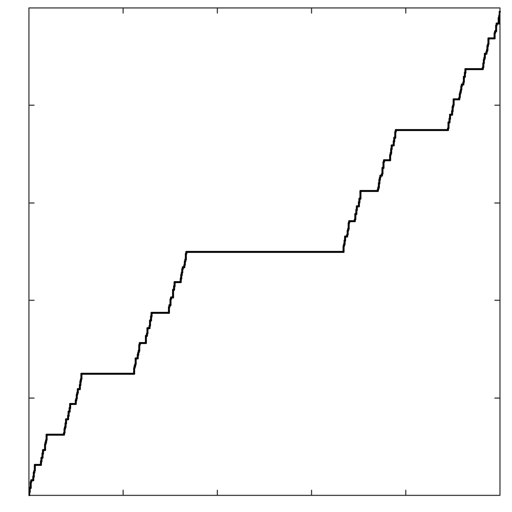
Figure 1: Cantor ladder

Recall that we deal with a Green Gaussian process, so the integral equation (60) is equivalent to the boundary value problem

$${\cal L}u=\lambda\mathfrak{m}u\quad{\rm on}\quad[0,1],\qquad u\in{\cal D}({\cal L}),$$ (62)

where $\lambda=\mu^{-1}$, ${\cal L}$ is defined in (13), and ${\cal D}({\cal L})$ is determined by the boundary conditions (14). For simplicity we assume that $p_{\ell}\equiv 1$.

We list the main steps in the research on the problem (62). More references can be found in [113].

For the simplest Sturm–Liouville operator ${\cal L}u\equiv-u^{\prime\prime}$, the exact power order $p$ of the eigenvalues growth was obtained by T. Fujita [57]. The one-term eigenvalues asymptotics in this case was obtained independently by J. Kigami and M.L. Lapidus [82] and by M.Z. Solomyak and E. Verbitsky [165]. A.I. Nazarov [113] generalized their result for the operators of arbitrary order.

Theorem 16 ([113, Theorem 3.1]).

Given self-similar probability measure $\mathfrak{m}$, define

$$\mathfrak{c}_{j}:=\mathfrak{r}_{j}\cdot|I_{j}|^{2\ell-1},\quad j=1,\dots,n,$$

and denote by $p$ the unique solution of the equation

$$\sum\limits_{j=1}^{n}\mathfrak{c}_{j}^{\frac{1}{p}}=1.$$

Evidently, $p\geq 2\ell$. Moreover, $p=2\ell$ only if $\mathfrak{m}$ is the Lebesgue measure.

Let $X$ be a Green Gaussian process, corresponding to the order $2\ell$ ODO.

1. If at least one ratio $\log(\mathfrak{c}_{i}^{-1})/\log(\mathfrak{c}_{j}^{-1})$ is irrational, the self-similarity of the measure $\mathfrak{m}$ is called non-arithmetic. In this case the counting function of eigenvalues to the integral equation (60) has purely power asymptotics:

$${\cal N}(\tau)\sim M\tau^{-\frac{1}{p}},\quad\tau\to 0,$$

where $M$ is some (unknown) constant.

2. If all quantities $\log(\mathfrak{c}_{j}^{-1})$ are mutually commensurable, the self-similarity of $\mathfrak{m}$ is called arithmetic. In this case

$${\cal N}(\tau)\sim\tau^{-\frac{1}{p}}\mathfrak{g}(\log(\tau^{-1})),\quad\tau\to 0,$$ (63)

where the function $\mathfrak{g}$ satisfies Condition A. Moreover, $\mathfrak{g}$ is periodic, and its period is equal to the greatest common divisor of $\log(\mathfrak{c}_{j}^{-1})$, $j=1,\dots,n$.

Remark 11.

The quantity $\gamma=\frac{2\ell-1}{p-1}$ is called spectral dimension of order $2\ell-1$ of the self-similar measure $\mathfrak{m}$. It is shown in [113, Theorem 5.3] that $\gamma\leq\alpha$ (recall that $\alpha$ is the Hausdorff dimension of the support of $\mathfrak{m}$), and $\gamma=\alpha$ if and only if $\mathfrak{r}_{j}=|I_{j}|^{\alpha}$ for any $j=1,\dots,n$. In particular, this is the case for the standard Cantor measure, where $\gamma=\alpha=\frac{\log(2)}{\log(3)}$.

Remark 12.

Theorem 16 was generalized in several directions. Namely, the problem (62) was considered under the following assumptions:

1. ${\cal L}u\equiv-u^{\prime\prime}$, and $\mathfrak{m}$ is the distributional derivative of the Minkowski question-mark function, see [162]. In this case $\mathfrak{m}$ is a non-affine self-similar measure, i.e. relation (61) holds with non-affine diffeomorphisms $S_{j}$, namely,

   $$n=2,\quad S_{1}(t)=\frac{t}{t+1},\quad S_{2}(t)=\frac{1}{2-t}.$$

   In [162, Theorem 3.2], two-sided estimates for the eigenvalues of counting function were obtained:

   $${\cal N}(\tau)\asymp\tau^{\frac{\mathfrak{d}}{\mathfrak{d}+1}},\quad\tau\to 0;\qquad\mathfrak{d}=\frac{1}{2}\Big{(}\int\limits_{0}^{1}\log_{2}(1+t)\,d\mathfrak{m}\Big{)}^{-1}.$$

2. ${\cal L}u\equiv-u^{\prime\prime}$, and $\mathfrak{m}$ is a self-conformal measure, i.e. $S_{j}$ in the relation (61) are non-affine diffeomorphisms mapping $(0,1)$ onto $I_{j}$, subject to some additional assumptions, see [55], [56];

3. $\mathfrak{m}$ is a sign-changing self-similar distribution, see [174], [175];

4. ${\cal L}$ is a so-called measure geometric Krein–Feller operator related to two self-similar measures, see [54] and references therein.

Up to our knowledge, the generalizations mentioned in items 3 and 4 have not found an application in the study of small ball probabilities yet.

Using general results of Theorem 16 and Lemma 62, the logarithmic small ball asymptotics in $L_{2}[0,1;d\mathfrak{m}]$ were obtained in [113] for several classical Green Gaussian processes.

The statement of “arithmetic” part 2 in Theorem 16 does not exclude the “degenerate” case where function $\mathfrak{g}$ in (63) is a constant, i.e. ${\cal N}(\tau)$ has classical power asymptotics. It was conjectured in [113] that it is not the case, i.e. $\mathfrak{g}\neq const$ for any non-Lebesgue arithmetically self-similar measure $\mathfrak{m}$.

A.A. Vladimirov and I.A. Sheipak [175] confirmed this conjecture for the standard Cantor measure and ${\cal L}u\equiv-u^{\prime\prime}$ using computer-assisted proof. Later [178] they succeeded to give a complete characterization of the function $\mathfrak{g}$ under assumption that $\mathfrak{m}$ is a so-called even Cantor-type measure.

Theorem 17 ([178, Section 5]).

Suppose that $\mathfrak{m}$ is an even Cantor-type measure, that is, for all $j=1,\dots,n$, the lengths $|I_{j}|$ are equal, the gaps between neighbor intervals $I_{j}$ are equal (and non-zero), and the weights $\mathfrak{r}_{j}$ are equal. Let ${\cal L}u\equiv-u^{\prime\prime}$. Then the function $\mathfrak{g}$ in (63) satisfies the relation

$$\mathfrak{g}(t)=\exp(-\tfrac{t}{p})\mathfrak{s}(t),$$ (64)

where $\mathfrak{s}$ is some purely singular non-decreasing function (i.e. a primitive of a singular measure).

In [172] this result was transferred to the fourth order operator ${\cal L}$.

N.V. Rastegaev [151], [153] obtained formula (64) for ${\cal L}u\equiv-u^{\prime\prime}$ and arbitrary arithmetically self-similar measure $\mathfrak{m}$ under the only assumption: all gaps between neighbor intervals $I_{j}$ are non-zero. Further generalization (in particular, for the higher order operator ${\cal L}$) is an interesting open problem.

All previous examples generate the eigenvalues asymptotics (58) with $\Psi\equiv 1$. A general form of (58) arises, for instance, when considering tensor products. We describe briefly corresponding results obtained by N.V. Rastegaev [152]. Let ${\cal K}_{1}$ and ${\cal K}_{2}$ be positive (compact, self-adjoint) operators. Suppose that

$${\cal N}_{{\cal K}_{1}}(\tau)\sim\tau^{-\frac{1}{p_{1}}}\Phi_{1}(\tau^{-1})\mathfrak{g}_{1}(\log(\tau^{-1})),\quad\tau\to 0,$$ (65)

where $p_{1}>1$, $\Phi_{1}$ is a SVF, and $\mathfrak{g}_{1}$ is a continuous positive $T_{1}$-periodic function.

If ${\cal N}_{{\cal K}_{2}}(\tau)=O(\tau^{-\frac{1}{p_{2}}})$ as $\tau\to 0$, with $p_{2}>p_{1}$ then

$${\cal N}_{\otimes}(\tau)\sim\tau^{-\frac{1}{p_{1}}}\Phi_{1}(\tau^{-1})\mathfrak{g}^{*}(\log(\tau^{-1})),\quad\tau\to 0,$$

where $\mathfrak{g}^{*}$ is a continuous positive $T_{1}$-periodic function.

Remark 13.

It is shown in [152, Remark 2] that in general case $\mathfrak{g}^{*}$ can degenerate into constant even if $\mathfrak{g}_{1}$ is not a constant. However, if $\mathfrak{g}_{1}$ has the form given in Theorem 17 then $\mathfrak{g}^{*}$ also has such a form.

Suppose now that ${\cal K}_{2}$ satisfies a similar relation

$${\cal N}_{{\cal K}_{2}}(\tau)\sim\tau^{-\frac{1}{p_{2}}}\Phi_{2}(\tau^{-1})\mathfrak{g}_{2}(\log(\tau^{-1})),\quad\tau\to 0$$

($p_{2}>1$, $\Phi_{2}$ is a SVF, and $\mathfrak{g}_{2}$ is a continuous positive $T_{2}$-periodic function), and let $p_{1}=p_{2}=p$. Then the asymptotics of ${\cal N}_{\otimes}(\tau)$ as $\tau\to 0$ is more complicated and depends on convergence of integrals (55) and, if they both diverge, on the commensurability of $T_{1}$ and $T_{2}$. In particular, if both integrals (55) diverge and $T_{1}=T_{2}=T$ then

$${\cal N}_{\otimes}(\tau)\sim\tau^{-\frac{1}{p}}(\Phi_{1}*\Phi_{2})(\tau^{-1})\mathfrak{g}_{\otimes}(\log(\tau^{-1})),\quad\tau\to 0,$$

(the Mellin convolution of SVFs is defined in (53)), where $\mathfrak{g}_{\otimes}$ is an explicit (though complicated) continuous positive $T$-periodic function.

Remark 14.

The question of non-constancy of $\mathfrak{g}_{\otimes}$ remains open even in the case where both $\mathfrak{g}_{1}$ and $\mathfrak{g}_{2}$ have the form given in Theorem 17.

5.5 Slowly varying asymptotics

In this subsection we consider processes with super-power decay of eigenvalues. More exactly, we assume that the counting function ${\cal N}(\tau)$ is slowly varying at zero. Corresponding analog of the relation (47) reads as follows:

Lemma 4 ([115, Theorem 2]).

Let $(\mu_{k})$, $k\in\mathbb{N}$, be a positive sequence with counting function ${\cal N}(\tau)$, and let

$${\cal N}(\tau)\sim\Phi(\tau^{-1}),\quad\tau\to 0,$$ (66)

where $\Phi$ is a SVF. Then, as $\varepsilon\to 0$,

$$\log\mathbb{P}\Big{\{}\sum_{k=1}^{\infty}\mu_{k}\xi_{k}^{2}\leq\varepsilon^{2}\Big{\}}\sim-\frac{\Theta(\gamma)}{2}:=-\frac{(\Phi*{\bf 1})(\gamma)}{2}\equiv-\frac{1}{2}\int\limits_{1}^{\gamma}\Phi(\sigma)\sigma^{-1}d\sigma,$$

where $\gamma=\gamma(r)$ satisfies the relation

$$\frac{\Phi(\gamma)}{2\gamma}\sim\varepsilon^{2},\qquad\varepsilon\to 0.$$

Remark 15.

As it was mentioned in Subsection 5.3, $\Theta$ is a SVF, cf. (53).

The first examples of Gaussian processes satisfying (66) arose in [62], where the case $\log(\mu_{k})\sim-k^{\alpha}\Psi(k)$ as $k\to\infty$ with a SVF $\Psi$ was considered.

The relation (66) is typical for the processes with smooth covariances. In [115], a set of smooth stationary Gaussian processes ${\cal R}_{C,\alpha}$ ($C,\alpha>0$) was considered. These processes have zero mean-value and the spectral density

$${\bf m}_{C,\alpha}(\xi)=\exp(-C|\xi|^{\alpha}),\qquad\xi\in\mathbb{R}.$$ (67)

For instance, it is well known that

$$G_{{\cal R}_{C,1}}(s,t)=\frac{C}{\pi(C^{2}+(s-t)^{2})},\qquad G_{{\cal R}_{C,2}}(s,t)=\frac{1}{2\sqrt{\pi C}}\exp\left(-\frac{(s-t)^{2}}{4C}\right).$$

The spectral asymptotics for the integral operators with kernels of this type was treated in remarkable paper [180]. The following relation for the counting function can be extracted from [180, Theorems 1 and 2]: as $\tau\to 0$, we have

$${\cal N}(\tau)\sim\Phi(\tau^{-1})\equiv\begin{cases}\frac{1}{\pi_{\displaystyle\vphantom{1}}C^{\frac{1}{\alpha}}}\cdot\log^{\frac{1}{\alpha}}(\tau^{-1}),&\ \alpha<1;\\ \frac{1}{\pi_{\displaystyle\vphantom{1}}\mathfrak{C}}\cdot\log(\tau^{-1}),&\ \alpha=1;\\ \frac{\alpha}{2\alpha-2}\cdot\frac{\log(\tau^{-1})}{\log(\log(\tau^{-1}))},&\ \alpha>1.\end{cases}$$

Here

$$\mathfrak{C}=\frac{{\bf K}\bigl{(}\mbox{sech}\bigl{(}\frac{\pi}{2C}\bigr{)}\bigr{)}}{{\bf K}\bigl{(}\tanh\bigl{(}\frac{\pi}{2C}\bigr{)}\bigr{)}},$$

while $\bf K$ is the complete elliptic integral of the first kind.

So, Lemma 4 yields the following relation as $\varepsilon\to 0$:

$$\log{\mathbb{P}}\left\{\|{\cal R}_{C,\alpha}\|_{2,[0,1]}\leq\varepsilon\right\}\sim\begin{cases}-\,\big{(}\frac{2}{C}\big{)}^{\frac{1}{\alpha}}\,\frac{\alpha}{(\alpha+1)\pi_{\displaystyle\vphantom{1}}}\cdot\log^{\frac{\alpha+1}{\alpha}}(\varepsilon^{-1}),&\ \alpha<1;\\ -\,\frac{1}{\pi_{\displaystyle\vphantom{1}}\mathfrak{C}}\cdot\log^{2}(\varepsilon^{-1}),&\ \alpha=1;\\ -\,\frac{\alpha}{2\alpha-2}\cdot\frac{\log^{2}(\varepsilon^{-1})}{\log(\log(\varepsilon^{-1}))},&\ \alpha>1.\end{cases}$$

Remark 16.

Notice that the order of logarithmic $L_{2}$-small ball asymptotics in the latter case depends neither on $C$ nor even on $\alpha$. The same effect was found in [8] for the sup-norm.

F. Aurzada, F. Gao, Th. Kühn, W.V. Li and Q.-M. Shao [7] investigated the small ball behavior in $L_{2}$- and sup-norms of smooth self-similar Gaussian processes $X_{\alpha,\beta}$ with the covariance function

$$G_{X_{\alpha,\beta}}(t,s)=\frac{t^{\alpha}s^{\alpha}}{(t+s)^{2\beta+1}}.$$ (68)

In particular, it was shown that under natural assumption $\alpha>\beta>-\frac{1}{2}$ we have

$$\log{\mathbb{P}}\left\{\|X_{\alpha,\beta}\|_{2,[0,1]}\leq\varepsilon\right\}\sim-\,\frac{1}{3(\alpha-\beta)\pi^{2}}\,\log^{3}(\varepsilon^{-1}),\quad\varepsilon\to 0.$$ (69)

Remark 17.

The method of [7] is based on the estimates of entropy numbers of a linear operator generating the process, see [88]. We notice that the spectral asymptotics for the operator with kernel (68) was obtained many years ago by A.A. Laptev [91]. So, formula (69) can be obtained from the result of [91] and Lemma 4.

Another class of problems where the relation (66) appears is related to the Green Gaussian process in the space $L_{2}[0,1;d\mathfrak{m}]$ with very “poor” measure $\mathfrak{m}$. We describe here (not in a full generality) corresponding class of degenerate self-similar measures on $[0,1]$, see [161], [129].

Let $0<t_{1}<\ldots<t_{n}<1$, $n\geq 2$, be a partition of the segment $[0,1]$. We select one of intervals between these points $I=(t_{k},t_{k+1})$ and define the affine function $S$ mapping $(0,1)$ onto $I$. Consider also positive numbers (weights) $a_{j}>0$, $j=1,\ldots,n$, and $\mathfrak{r}>0$ such that $\sum\limits_{j}a_{j}+\mathfrak{r}=1$.

It is not difficult to show (see, e.g., [161]), that there is a unique probability measure $\mathfrak{m}$ such that for any Lebesgue-measurable set ${\cal E}\subset[0,1]$

$$\mathfrak{m}({\cal E})=\mathfrak{r}\cdot\mathfrak{m}(S^{-1}({\cal E}))+\sum\limits_{t_{j}\in{\cal E}}a_{j}.$$ (70)

In contrast with self-similar measures considered in Subsection 5.4, the measure $\mathfrak{m}$, defined by relation (70), is discrete. Its support has a unique accumulation point $\widehat{x}$. Straightforward calculation shows that

$$\widehat{x}=\dfrac{t_{k}}{1-|I|}.$$ (71)

The primitive of $\mathfrak{m}$ is a piecewise constant function. Fig. 2 shows its graph for the following values of parameters: $n=2$; $t_{1}=0.3$, $t_{2}=0.8$; $a_{1}=\frac{1}{3}$, $a_{2}=\frac{1}{3}$, $\mathfrak{r}=\frac{1}{3}$. Formula (71) gives $\hat{x}=0.6$.

Figure 2: The primitive of a degenerate self-similar measure

Remark 18.

Evidently, the Hausdorff dimension of the support of degenerate self-similar measure is equal to zero. Therefore, the spectral dimension of $\mathfrak{m}$ (see Remark 11) is also equal to zero.

The first result on the eigenvalues asymptotics for the boundary value problem (62) with degenerate self-similar measure $\mathfrak{m}$ was obtained by A.A. Vladimirov and I.A. Sheipak [176] in the case ${\cal L}u\equiv-u^{\prime\prime}$. In [129], [177] this result was generalized for the operators of arbitrary order. Using these results and Lemma 4, the logarithmic small ball asymptotics in $L_{2}[0,1;d\mathfrak{m}]$ was obtained in [129] for several classical Green Gaussian processes.

Theorem 18 ([129, Proposition 4.3]).

Let $\mathfrak{m}$ be a degenerate self-similar measure described above. Let $X$ be a Green Gaussian process, corresponding to the order $2\ell$ ODO. Then

$$\log{\mathbb{P}}\{\|X\|_{2,[0,1];\,d\mathfrak{m}}\leq\varepsilon\}\sim-\,\frac{n}{\log(\mathfrak{c}^{-1})}\,\log^{2}(\varepsilon^{-1}),\quad\varepsilon\to 0,$$

where $\mathfrak{c}=\mathfrak{r}\cdot|I|^{2\ell-1}$.

Tensor products of Gaussian processes with eigenvalues counting functions, which are slowly varying at zero, were considered by A.I. Karol’ and A.I. Nazarov [76].

Theorem 19 ([76, Theorem 3.2]).

Let ${\cal K}_{1}$ and ${\cal K}_{2}$ be positive (compact, self-adjoint) operators. Suppose that

$${\cal N}_{{\cal K}_{1}}(\tau)\sim\Phi_{1}(\tau^{-1}),\qquad{\cal N}_{{\cal K}_{2}}(\tau)\sim\Phi_{2}(\tau^{-1}),\quad\tau\to 0,$$ (72)

where $\Phi_{1}$ and $\Phi_{2}$ are unbounded and non-decreasing SVFs. Then we have

$${\cal N}_{\otimes}(\tau)\sim(\Phi_{1}\star\Phi_{2})(\tau^{-1}),\qquad\tau\to 0,$$ (73)

where

$$(\Phi\star\Psi)(s)=\int\limits_{1}^{s}\Phi(s\sigma^{-1})d\Psi(\sigma)$$ (74)

is the so-called asymptotic convolution of SVFs.

Using general results of Theorem 19 and Lemma 4, the logarithmic $L_{2}$-small ball asymptotics were obtained in [76] for several fields-products with marginal processes described above.

Appendix.
$L_{2}$-small ball asymptotics for concrete processes

Process	Logarithmic asymptotics	Asympt. up to constant	Exact asymptotics
Wiener process, $W$			[28]8
Brownian bridge, $B$			[5]88
Ornstein-Uhlenbeck, $U$	[92]	[120]	[112];  [58];;;
Centered Wiener process, $\overline{W}$			[11]8
Centered Brownian bridge, $\overline{B}$			[11]8
Other Green Gaussian processes of the second order			[131];  [114]; [142];  [70]8;
Weighted Green Gaussian processes of the second order		[92]; [43];	[112];  [58];8 [130];  [127]; [142];  [9];88 [132];  [122];
$m$-times integrated Wiener process, $W_{m}^{[\beta_{1},\ldots,\beta_{m}]}$	[81]; [31];	[11]; [61]; [120]	[58];8  [59];8 [112]
$m$-times integrated Brownian bridge, $B_{m}^{[\beta_{1},\ldots,\beta_{m}]}$		[11]; [120];	[58];8  [112];
$m$-times integrated Ornstein–Uhlenbeck, $U_{m}^{[\beta_{1},\ldots,\beta_{m}]}$		[120]	[112]
Other Green Gaussian processes of the higher order		[120];; [11]8;	[112];  [141]; [114];  [142]; [143];  [122];
Weighted Green Gaussian processes of the higher order			[127];  [128];

Process	Logarithmic asymptotics	Asympt. up to constant	Exact asymptotics
Detrended Green processes		[3]88	[84];8  [139];
Finite-dimensional perturbations			[116];  [125]; [138]
Fractional Brownian motion (fBm), $W^{H}$	[26]8	[32]8
$m$-times integrated fBm	[121]	[34]; [37]8;
Other fractional-Green processes		[35];   [118]; [37]8
Riemann–Liouville process and bridge		[33]8
Other fractional processes and fields	[121];  [143]; [67];8  [100];
Smooth processes	[62];8  [115]; [7]88
Fractional processes with variable Hurst index	[77];8  [75]8;
Processes with self-similar measure	[113];   [129]; [56]; [153];
Brownian sheet	[39]8		[53]8
Integrated Brownian sheet	[78]8		[53]8
Other fields-products	[78];8  [62];8 [63];8  [76];8 [90]; [152];		[156];  [157];

References

- [1] X. Ai. A note on Karhunen–Loève expansions for the demeaned stationary Ornstein–Uhlenbeck process. Statistics & Probability Letters, 117:113–117, 2016.
- [2] X. Ai and W. Li. Karhunen–Loève expansions for the -th order detrended Brownian motion. Science China Mathematics, 57(10):2043–2052, 2014.
- [3] X. Ai, W. Li, and G. Liu. Karhunen–Loève expansions for the detrended Brownian motion. Statistics & Probability Letters, 82(7):1235–1241, 2012.
- [4] J.M.P. Albin. Minima of -valued Gaussian processes. The Annals of Probability, 24(2):788–824, 1996.
- [5] T. Anderson and D. Darling. Asymptotic theory of certain “goodness of fit” criteria based on stochastic processes. The Annals of Mathematical Statistics, 23(2):193–212, 1952.
- [6] F. Aurzada. On the lower tail probabilities of some random sequences in . Journal of Theoretical Probability, 20(4):843–858, 2007.
- [7] F. Aurzada, F. Gao, Th. Kühn, W.V. Li, and Q.-M. Shao. Small deviations for a family of smooth Gaussian processes. Journal of Theoretical Probability, 26(1):153–168, 2013.
- [8] F. Aurzada, I.A. Ibragimov, M.A. Lifshits, and J.H. van Zanten. Small deviations of smooth stationary Gaussian processes. Theory of Probability & Its Applications, 53(4):697–707, 2009.
- [9] M. Barczy and E. Iglói. Karhunen-Loève expansions of -Wiener bridges. Central European Journal of Mathematics, 9(1):65–84, 2011.
- [10] M. Barczy and R.L. Lovas. Karhunen–Loève expansion for a generalization of Wiener bridge. Lithuanian Mathematical Journal, 58(4):341–359, 2018.
- [11] L. Beghin, Ya.Yu. Nikitin, and E. Orsingher. Exact small ball constants for some Gaussian processes under the -norm. Zapiski Nauchnykh Seminarov POMI, 298:5–21, 2003. English transl.: Journal of Mathematical Sciences, 128(1):2493–2502, 2005.
- [12] A. Benassi, S. Cohen, and J. Istas. Identifying the multifractional function of a Gaussian process. Statistics & Probability Letters, 39(4):337–345, 1998.
- [13] G. Birkhoff. Boundary value and expansion problems of ordinary linear differential equations. Transactions of the American Mathematical Society, 9(4):373–395, 1908.
- [14] G. Birkhoff. On the asymptotic character of the solutions of certain linear differential equations containing a parameter. Transactions of the American Mathematical Society, 9(2):219–231, 1908.
- [15] M.S. Birman and M.Z. Solomjak. Asymptotics of the spectrum of pseudodifferential operators with anisotropic-homogeneous symbols. Vestnik LGU, 13:13–21, 1977. [Russian]. English transl.: Vestnik Leningrad Univ. Math., 10:237–247, 1982.
- [16] M.S. Birman and M.Z. Solomjak. Asymptotics of the spectrum of pseudodifferential operators with anisotropic-homogeneous symbols. II. Vestnik LGU, 3:5–10, 1979. [Russian]. English transl.: Vestnik Leningrad Univ. Math., 12:155–161, 1980.
- [17] M.S. Birman and M.Z. Solomyak. Asymptotic behavior of the spectrum of weakly polar integral operators. Izvestiya Akademii Nauk USSR. Seriya Matematicheskaya, 34(6):1143–1158, 1970. [Russian]. English transl.: Math. USSR-Izv., 4(5):1151–1168, 1970.
- [18] M.S. Birman and M.Z. Solomyak. Quantitative analysis in Sobolev imbedding theorems and applications to spectral theory. In Proceedings of X Summer Mathematical School. Yu.A. Mitropol’skiy and A.F. Shestopal (Eds), pages 5–189, 1974. [Russian]. English transl.: AMS Translations, Series 2, 114, Providence, R.I., 1980.
- [19] M.S. Birman and M.Z. Solomyak. On the negative discrete spectrum of a periodic elliptic operator in a waveguide-type domain, perturbed by a decaying potential. Journal d’Analyse Mathématique, 83(1):337–391, 2001.
- [20] M.S. Birman and M.Z. Solomyak. Spectral theory of self-adjoint operators in Hilbert space. Second edition, revised and extended. Lan’, St.Petersburg, 2010. [Russian]. English transl. of the first edition: Mathematics and Its Applications. Soviet Series, 5, Kluwer, Dordrecht etc. 1987.
- [21] Ch. Borell. A note on Gauss measures which agree on small balls. Annales de l’IHP Probabilités et statistiques, 13(3):231–238, 1977.
- [22] A.A. Borovkov and A.A. Mogul’skii. On probabilities of small deviations for random processes. Trudy Instituta Matematiki Sibirskogo Otdeleniya AN SSSR, 13:147–168, 1989. [Russian].
- [23] A.A. Borovkov and P.S. Ruzankin. On small deviations of series of weighted random variables. Journal of Theoretical Probability, 21(3):628–649, 2008.
- [24] A.A. Borovkov and P.S. Ruzankin. Small deviations of series of independent positive random variables with weights close to exponential. Siberian Advances in Mathematics, 18(3):163–175, 2008.
- [25] V.V. Borzov. Quantitative characteristics of singular measures. In Spectral Theory and Wave Processes, volume 4 of Problems of Mathematical Physics, pages 42–47. Leningrad University Publisher, 1970. [Russian]. English transl.: volume 4 of Topics in Mathematical Physics, pages 37–42, Springer, Boston, 1971.
- [26] J.C. Bronski. Small ball constants and tight eigenvalue asymptotics for fractional Brownian motions. Journal of Theoretical Probability, 16(1):87–100, 2003.
- [27] C.-H. Cai, J.-Q. Hu, and Y.-L. Wang. Asymptotics of Karhunen–Loève eigenvalues for sub-fractional Brownian motion and its application. Fractal and Fractional, 5(4):226, 2021.
- [28] R. Cameron and W. Martin. The Wiener measure of Hilbert neighborhoods in the space of real continuous functions. Journal of Mathematics and Physics, 23(1-4):195–209, 1944.
- [29] R. Carmona. Tensor products of Gaussian measures. In Vector Space Measures and Applications I, volume 644 of Lecture Notes in Mathematics, pages 96–124. Springer Berlin Heidelberg, 1977.
- [30] R. Carmona and S. Chevet. Tensor Gaussian measures on . Journal of Functional Analysis, 33(3):297–310, 1979.
- [31] X. Chen and W. Li. Quadratic functionals and small ball probabilities for the -fold integrated Brownian motion. The Annals of Probability, 31(2):1052–1077, 2003.
- [32] P.Yu. Chigansky and M.L. Kleptsyna. Exact asymptotics in eigenproblems for fractional Brownian covariance operators. Stochastic Processes and their Applications, 128(6):2007–2059, 2018.
- [33] P.Yu. Chigansky and M.L. Kleptsyna. Sharp asymptotics in a fractional Sturm–Liouville problem. Fractional Calculus and Applied Analysis, 24(3):715–738, 2021.
- [34] P.Yu. Chigansky, M.L. Kleptsyna, and D.A. Marushkevych. Exact spectral asymptotics of fractional processes. arXiv:1802.09045, 2018.
- [35] P.Yu. Chigansky, M.L. Kleptsyna, and D.A. Marushkevych. Mixed fractional Brownian motion: A spectral take. Journal of Mathematical Analysis and Applications, 482(2):123558, 2020.
- [36] P.Yu. Chigansky, M.L. Kleptsyna, and D.A. Marushkevych. On the eigenproblem for Gaussian bridges. Bernoulli, 26(3):1706–1726, 2020.
- [37] P.Yu. Chigansky, M.L. Kleptsyna, A.I. Nazarov, and N.V. Rastegaev. Spectral asymptotics for a class of integro-differential equations arising in the theory of integrated fractional Gaussian processes. Technical report, in preparation, 2023.
- [38] D. Cox. On the existence of natural rate of escape functions for infinite dimensional Brownian motions. The Annals of Probability, 10(3):623–638, 1982.
- [39] E. Csáki. On small values of the square integral of a multiparameter Wiener process. In Statistics and Probability. Proceedings of the 3rd Pannonian Symposium on Mathematical Statistics, pages 19–26. D. Reidel Publishing Company, 1982.
- [40] R. Davis and S. Resnick. Extremes of moving averages of random variables with finite endpoint. The Annals of Probability, 19(1):312–328, 1991.
- [41] P. Deheuvels. Karhunen–Loève expansions of mean-centered Wiener processes. In High Dimensional Probability. Proceedings of the Fourth International Conference, IMS Lecture Notes — Monograph Series, Vol. 51, pages 62–76. IMS, Beachwood, OH, 2006.
- [42] P. Deheuvels. A Karhunen–Loève expansion for a mean-centered Brownian bridge. Statistics & Probability Letters, 77(12):1190–1200, 2007.
- [43] P. Deheuvels and G. Martynov. Karhunen–Loève expansions for weighted Wiener processes and Brownian bridges via Bessel functions. In High Dimensional Probability III, volume 55 of Progress in probability, pages 57–93. Springer Basel, 2003.
- [44] P. Deheuvels, G. Peccati, and M. Yor. On quadratic functionals of the Brownian sheet and related processes. Stochastic Processes and their Applications, 116(3):493–538, 2006.
- [45] A. Dembo, E. Mayer-Wolf, and O. Zeituni. Exact behavior of Gaussian seminorms. Statistics & Probability Letters, 23(3):275–280, 1995.
- [46] S. Dereich. Small ball probabilities around random centers of Gaussian measures and applications to quantization. Journal of Theoretical Probability, 16(2):427–449, 2003.
- [47] C. Donati-Martin and M. Yor. Fubini’s theorem for double Wiener integrals and the variance of the Brownian path. Annales de l’Institut Henri Poincaré. Probabilités et statistiques, 27(2):181–200, 1991.
- [48] N. Dunford and J.T. Schwartz. Linear Operators. Part III: Spectral Operators. Wiley, New York. With the assistance of William G. Bade and Robert G. Bartle, 1971.
- [49] T. Dunker, M.A. Lifshits, and W. Linde. Small deviation probabilities of sums of independent random variables. In High dimensional probability, volume 43 of Progress in probability, pages 59–74. Springer Basel, 1998.
- [50] J. Durbin. Weak convergence of the sample distribution function when parameters are estimated. The Annals of Statistics, 1(2):279–290, 1973.
- [51] V.R. Fatalov. Constants in the asymptotics of small deviation probabilities for Gaussian processes and fields. Russian Mathematical Surveys, 58(4):725–772, 2003.
- [52] F. Ferraty and Ph. Vieu. Nonparametric functional data analysis: theory and practice, volume 76 of Springer Series in Statistics. Springer, NY, 2006.
- [53] J.A. Fill and F. Torcaso. Asymptotic analysis via Mellin transforms for small deviations in -norm of integrated Brownian sheets. Probability theory and related fields, 130(2):259–288, 2004.
- [54] U. Freiberg. Refinement of the spectral asymptotics of generalized Krein Feller operators. Forum Mathematicum, 23:427–445, 2011.
- [55] U.R. Freiberg and N.V. Rastegaev. On spectral asymptotics of the Sturm–Liouville problem with self-conformal singular weight with strong bounded distortion property. Zapiski Nauchnykh Seminarov POMI, 477:129–135, 2018. [Russian]. English transl.: Journal of Mathematical Sciences, 244(6):1010–1014, 2020.
- [56] U.R. Freiberg and N.V. Rastegaev. On spectral asymptotics of the Sturm–Liouville problem with self-conformal singular weight. Siberian Mathematical Journal, 61(5):901–912, 2020.
- [57] T. Fujita. A fractional dimension, self-similarity and a generalized diffusion operator. In Probabilistic methods in mathematical physics, Proceedings of Taniguchi International Symposium, pages 83–90. Tokyo, Kinokuniya, 1987.
- [58] F. Gao, J. Hannig, T. Lee, and F. Torcaso. Laplace transforms via Hadamard factorization. Electronic Journal of Probability, 8:1–20, 2003.
- [59] F. Gao, J. Hannig, T.-Y. Lee, and F. Torcaso. Exact small balls of Gaussian processes. Journal of Theoretical Probability, 17(2):503–520, 2004.
- [60] F. Gao, J. Hannig, and F. Torcaso. Comparison theorems for small deviations of random series. Electronic Journal of Probability, 8:1–17, 2003.
- [61] F. Gao, J. Hannig, and F. Torcaso. Integrated Brownian motions and exact -small balls. The Annals of Probability, 31(3):1320–1337, 2003.
- [62] F. Gao and W. Li. Logarithmic level comparison for small deviation probabilities. Journal of Theoretical Probability, 20(1):1–23, 2007.
- [63] F. Gao and W. Li. Small ball probabilities for the Slepian Gaussian fields. Transactions of the American Mathematical Society, 359(3):1339–1350, 2007.
- [64] S. Graf, H. Luschgy, and G. Pagès. Functional quantization and small ball probabilities for Gaussian processes. Journal of Theoretical Probability, 16(4):1047–1062, 2003.
- [65] J. Hoffmann-Jørgensen. Bounds for the Gaussian measure of a small ball in a Hilbert space. Technical report, Aarhus Universitet, Matematisk Institut, 1976.
- [66] J. Hoffmann-Jørgensen, L.A. Shepp, and R.M. Dudley. On the lower tail of Gaussian seminorms. The Annals of Probability, 7(2):319–342, 1979.
- [67] S.Y. Hong, M.A. Lifshits, and A.I. Nazarov. Small deviations in -norm for Gaussian dependent sequences. Electronic Communications in Probability, 21(41):1–9, 2016.
- [68] J.E. Hutchinson. Fractals and self similarity. Indiana University Mathematics Journal, 30(5):713–747, 1981.
- [69] I.A. Ibragimov. The probability of a Gaussian vector with values in a Hilbert space hitting a ball of small radius. Zapiski Nauchnykh Seminarov LOMI, 85:75–93, 1979. [Russian]. English transl.: Journal of Soviet Mathematics, 20(3):2164–2175, 1982.
- [70] S. Jin. Gaussian processes: Karhunen–Loève expansion, small ball estimates and applications in time series models. PhD thesis, University of Delaware, 2014.
- [71] M. Kac, J. Kiefer, and J. Wolfowitz. On tests of normality and other tests of goodness of fit based on distance methods. The Annals of Mathematical Statistics, 26(2):189–211, 1955.
- [72] M. Kac and A.J.F. Siegert. An explicit representation of a stationary Gaussian process. The Annals of Mathematical Statistics, 18(3):438–442, 1947.
- [73] K. Karhunen. Zur spektraltheorie stochastischer prozesse. Annales Academiae Scientiarum Fennicae, 34, 1946. [German].
- [74] K. Karhunen. Über lineare methoden in der wahrscheinlichkeitsrechnung. Annales Academiae Scientiarum Fennicae, 47:3–79, 1947. [German].
- [75] A.I. Karol’. Singular values of compact pseudodifferential operators of variable order with nonsmooth symbol. Zapiski Nauchnykh Seminarov POMI, 519:67–104, 2022. [Russian].
- [76] A.I. Karol’ and A.I. Nazarov. Small ball probabilities for smooth Gaussian fields and tensor products of compact operators. Mathematische Nachrichten, 287(5-6):595–609, 2014.
- [77] A.I. Karol’ and A.I. Nazarov. Spectral analysis for some multifractional Gaussian processes. Russian Journal of Mathematical Physics, 28(4):488–500, 2021.
- [78] A.I. Karol’, A.I. Nazarov, and Ya.Yu. Nikitin. Small ball probabilities for Gaussian random fields and tensor products of compact operators. Transactions of the American Mathematical Society, 360(3):1443–1474, 2008.
- [79] A.A. Khartov and I.A. Limar. Asymptotic analysis in multivariate average case approximation with Gaussian kernels. Journal of Complexity, 70:101631, 2022.
- [80] D. Khoshnevisan. Multiparameter Processes: an introduction to random fields. Springer Science & Business Media, 2002.
- [81] D. Khoshnevisan and Z. Shi. Chung’s law for integrated Brownian motion. Transactions of the American Mathematical Society, 350(10):4253–4264, 1998.
- [82] J. Kigami and M.L. Lapidus. Weyl’s problem for the spectral distribution of Laplacians on p.c.f. self-similar fractals. Communications in Mathematical Physics, 158:93–125, 1993.
- [83] A.A. Kilbas, H.M. Srivastava, and J.J. Trujillo. Theory and applications of fractional differential equations, volume 204. Elsevier, 2006.
- [84] A.A. Kirichenko and Ya.Yu. Nikitin. Precise small deviations in of some Gaussian processes appearing in the regression context. Central European Journal of Mathematics, 12(11):1674–1686, 2014.
- [85] M.L. Kleptsyna and A. Le Breton. A Cameron-Martin type formula for general Gaussian processes – a filtering approach. Stochastics: An International Journal of Probability and Stochastic Processes, 72(3-4):229–251, 2002.
- [86] M.L. Kleptsyna, D.A. Marushkevych, and P.Yu. Chigansky. Asymptotic accuracy in estimation of a fractional signal in a small white noise. Automation and Remote Control, 81(3):411–429, 2020.
- [87] D.D. Kosambi. Statistics in function space. Journal of the Indian Mathematical Society, 7:76–88, 1943.
- [88] J. Kuelbs and W.V. Li. Metric entropy and the small ball problem for Gaussian measures. Journal of Functional Analysis, 116(1):133–157, 1993.
- [89] J. Kuelbs, W.V. Li, and W. Linde. The Gaussian measure of shifted balls. Probability Theory and Related Fields, 98(2):143–162, 1994.
- [90] Th. Kühn. Covering numbers of Gaussian reproducing kernel Hilbert spaces. Journal of Complexity, 27(5):489–499, 2011.
- [91] A.A. Laptev. Spectral asymptotic behavior of a class of integral operators. Mathematical Notes, 16:1038–1043, 1974.
- [92] W. Li. Comparison results for the lower tail of Gaussian seminorms. Journal of Theoretical Probability, 5(1):1–31, 1992.
- [93] W. Li and Q.-M. Shao. Gaussian processes: inequalities, small ball probabilities and applications. In Stochastic Processes: Theory and Methods. C.R. Rao and D. Shanbhag (Eds), volume 19 of Handbook of Statistics, pages 533–597. North-Holland/Elsevier, Amsterdam, 2001.
- [94] W.V. Li and W. Linde. Small ball problems for non-centered Gaussian measures. Probability and Mathematical Statistics, 14(2):231–251, 1993.
- [95] M.A. Lifshits. Gaussian random functions. Teor. Veroyatnost. i Mat. Statist. (TViMS), Kiev, 1995. [Russian]. English transl.: Kluwer, Dordrecht, 1995.
- [96] M.A. Lifshits. On the lower tail probabilities of some random series. The Annals of Probability, 25(1):424–442, 1997.
- [97] M.A. Lifshits. Asymptotic behavior of small ball probabilities. In Probability Theory and Mathematical Statistics. Proceedings of the Seventh Vilnius Conference, pages 453–468. VSP/TEV, 1999.
- [98] M.A. Lifshits. Lectures on Gaussian processes. Springer, 2012.
- [99] M.A. Lifshits. Bibliography of small deviation probabilities. https://airtable.com/shrMG0nNxl9SiGxII/tbl7Xj1mZW2VuYurm, 2023.
- [100] M.A. Lifshits and A.I. Nazarov. -small deviations for weighted stationary processes. Mathematika, 64(2):387–405, 2018.
- [101] M.A. Lifshits, A.I. Nazarov, and Ya.Yu. Nikitin. Tail behavior of anisotropic norms for Gaussian random fields. Comptes Rendus Mathematique, 336(1):85–88, 2003.
- [102] W. Linde. Comparison results for the small ball behavior of Gaussian random variables. In Probability in Banach Spaces, 9, Progress in probability, pages 273–292. Springer, 1994.
- [103] W. Linde and J. Rosinski. Exact behavior of Gaussian measures of translated balls in Hilbert spaces. Journal of Multivariate Analysis, 50(1):1–16, 1994.
- [104] J.V. Liu. Karhunen–Loève expansion for additive Brownian motions. Stochastic Processes and their Applications, 123(11):4090–4110, 2013.
- [105] M. Loève. Fonctions aléatoires du second ordre. In P. Lévy. Processus stochastiques et mouvement brownien, pages 367–420. Gauthier-Villars & , 1948. [French].
- [106] H. Luschgy and G. Pagès. Sharp asymptotics of the functional quantization problem for Gaussian processes. The Annals of Probability, 32(2):1574–1599, 2004.
- [107] A.S. Markus and V.I. Matsaev. Comparison theorems for spectra of linear operators and spectral asymptotics. Trudy Moskovskogo Matematicheskogo Obshchestva, 45:133–181, 1982. [Russian].
- [108] E. Mayer-Wolf and O. Zeituni. The probability of small Gaussian ellipsoids and associated conditional moments. The Annals of Probability, 21(1):14–24, 1993.
- [109] H. Minkowski. Zur Geometrie der Zahlen. In Verhandlungen des III Internationalen Mathematiker-Kongresses in Heidelberg, Berlin, pages 164–173. 1904. [German].
- [110] A.V. Nagaev and A.N. Startsev. Asymptotic properties of the distribution of an infinite quadratic form of Gaussian random variables. In Limit Theorems for Stochastic Processes and Statistical Conclusions, Work Collection, Tashkent, pages 144–160. 1981. [Russian].
- [111] M.A. Naimark. Linear Differential Operators. Second edition, Nauka, Moscow, 1969. [Russian]. English transl. of the first edition: Linear Differential Operators. Part I. F. Ungar Publ. Co. XIII, New York, 1967. Part II. F. Ungar Publ. Co. XV, New York, 1968.
- [112] A.I. Nazarov. On the sharp constant in the small ball asymptotics of some Gaussian processes under -norm. Journal of Mathematical Sciences, 117(3):4185–4210, 2003.
- [113] A.I. Nazarov. Logarithmic asymptotics of small deviations for some Gaussian processes in the -norm with respect to a self-similar measure. Zapiski Nauchnykh Seminarov POMI, 311:190–213, 2004. [Russian]. English transl.: Journal of Mathematical Sciences, 133(3):1314–1327, 2006.
- [114] A.I. Nazarov. Exact -small ball asymptotics of Gaussian processes and the spectrum of boundary-value problems. Journal of Theoretical Probability, 22(3):640–665, 2009.
- [115] A.I. Nazarov. Log-level comparison principle for small ball probabilities. Statistics & Probability Letters, 79(4):481–486, 2009.
- [116] A.I. Nazarov. On a set of transformations of Gaussian random functions. Teoriya Veroyatnostei i ee Primeneniya, 54(2):209–225, 2009. [Russian]. English transl.: Theory of Probability & Its Applications, 54(2):203–216, 2010.
- [117] A.I. Nazarov. Some lemmata on the perturbation of the spectrum. Russian Journal of Mathematical Physics, 27(3):378–381, 2020.
- [118] A.I. Nazarov. Spectral asymptotics for a class of integro-differential equations arising in the theory of fractional Gaussian processes. Communications in Contemporary Mathematics, 23(06):2050049, 2021.
- [119] A.I. Nazarov and F.L. Nazarov. On some property of convex functions and an inequality for the Vandermonde determinants. Journal of Mathematical Sciences, 120(2):1122–1124, 2004.
- [120] A.I. Nazarov and Ya.Yu. Nikitin. Exact -small ball behavior of integrated Gaussian processes and spectral asymptotics of boundary value problems. Probability Theory and Related Fields, 129(4):469–494, 2004.
- [121] A.I. Nazarov and Ya.Yu. Nikitin. Logarithmic -small ball asymptotics for some fractional Gaussian processes. Teoriya Veroyatnostei i ee Primeneniya, 49(4):695–711, 2004. [Russian]. English transl.: Theory of Probability & Its Applications, 49(4):645–658, 2005.
- [122] A.I. Nazarov and Ya.Yu. Nikitin. On small deviation asymptotics in of some mixed Gaussian processes. Mathematics, 6(4):55, 2018.
- [123] A.I. Nazarov and Ya.Yu. Nikitin. Gaussian processes centered at their online average, and applications. Statistics & Probability Letters, 170:109013, 2021.
- [124] A.I. Nazarov and Ya.Yu. Nikitin. Spectral equivalence of Gaussian random functions: operator approach. Bernoulli, 28(2):1448–1460, 2022.
- [125] A.I. Nazarov and Yu.P. Petrova. The small ball asymptotics in Hilbert norm for the Kac–Kiefer–Wolfowitz processes. Teoriya Veroyatnostei i ee Primeneniya, 60(3):482–505, 2015. [Russian]. English transl.: Theory of Probability & Its Applications, 60(3):460–480, 2016.
- [126] A.I. Nazarov and Yu.P. Petrova. -small ball asymptotics for some demeaned Gaussian processes. Technical report, in preparation, 2023.
- [127] A.I. Nazarov and R.S. Pusev. Exact small ball asymptotics in weighted -norm for some Gaussian processes. Journal of Mathematical Sciences, 163(4):409–469, 2009.
- [128] A.I. Nazarov and R.S. Pusev. Comparison theorems for the small ball probabilities of the Green Gaussian processes in weighted -norms. Algebra i Analiz, 25(3):131–146, 2013. [Russian]. English transl.: St. Petersburg Mathematical Journal, 25(3):455–466, 2014.
- [129] A.I. Nazarov and I.A. Sheipak. Degenerate self-similar measures, spectral asymptotics and small deviations of Gaussian processes. Bulletin of the London Mathematical Society, 44(1):12–24, 2012.
- [130] Ya.Yu. Nikitin and P.A. Kharinski. Sharp small deviation asymptotics in the -norm for a class of Gaussian processes. Zapiski Nauchnykh Seminarov POMI, 311:214–221, 2004. [Russian]. English transl.: Journal of Mathematical Sciences, 133(3):1328–1332, 2006.
- [131] Ya.Yu. Nikitin and E. Orsingher. Sharp small ball asymptotics for Slepian and Watson processes in Hilbert norm. Zapiski Nauchnykh Seminarov POMI, 320:120–128, 2004. [Russian]. English transl.: Journal of Mathematical Sciences, 137(1):4555-4560, 2006.
- [132] Ya.Yu. Nikitin and R.S. Pusev. Exact small deviation asymptotics for some Brownian functionals. Teoriya Veroyatnostei i ee Primeneniya, 57(1):98–123, 2012. [Russian]. English transl.: Theory of Probability & Its Applications, 57(1):60–81, 2013.
- [133] B.V. Pal’tsev. The asymptotics of the spectrum and eigenfunctions of convolution operators on a finite interval with a kernel with a homogeneous Fourier transform. Doklady Akademii Nauk SSSR, 218(1):28–31, 1974. [Russian].
- [134] B.V. Pal’tsev. Asymptotic behaviour of the spectra of integral convolution operators on a finite interval with homogeneous polar kernels. Izvestiya: Mathematics, 67(4):695–779, 2003.
- [135] A. Papageorgiou and G.W. Wasilkowski. On the average complexity of multivariate problems. Journal of Complexity, 6(1):1–23, 1990.
- [136] G. Peccati and M. Yor. Identities in law between quadratic functionals of bivariate Gaussian processes, through Fubini theorems and symmetric projections. In Approximation and probability, volume 72 of Banach Center Publications, pages 235–250. Polish Academy of Sciences, Institute of Mathematics, 2006.
- [137] R.-F. Peltier and J. Levy Véhel. Multifractional Brownian motion: definition and preliminary results. Technical report, INRIA, 1995.
- [138] Yu.P. Petrova. Exact -small ball asymptotics for some Durbin processes. Zapiski Nauchnykh Seminarov POMI, 466:211–233, 2017. [Russian]. English transl.: Journal of Mathematical Sciences, 244(5):842-857, 2020.
- [139] Yu.P. Petrova. Spectral asymptotics for problems with integral constraints. Mathematical Notes, 102(3):369–377, 2017.
- [140] Yu.P. Petrova. -small ball asymptotics for a family of finite-dimensional perturbations of Gaussian functions. Zapiski Nauchnykh Seminarov POMI, Ya.Yu. Nikitin’s memorial volume, 501:236–258, 2021. [Russian].
- [141] R.S. Pusev. Small deviations for Matérn random fields and processes in the Hilbert norm. Doklady Mathematics, 78(2):778–780, 2008.
- [142] R.S. Pusev. Asymptotics of small deviations of the Bogoliubov processes with respect to a quadratic norm. Theoretical and Mathematical Physics, 165(1):1348–1357, 2010.
- [143] R.S. Pusev. Small deviations asymptotics for Matérn processes and fields under weighted quadratic norm. Teoriya Veroyatnostei i ee Primeneniya, 55(1):187–195, 2010. [Russian]. English transl.:Theory of Probability & Its Applications, 55(1):164–172, 2011.
- [144] J.-R. Pycke. Une généralisation du développement de Karhunen–Loève du pont brownien. Comptes Rendus de l’Académie des Sciences-Series I-Mathematics, 333(7):685–688, 2001. [French].
- [145] J.-R. Pycke. Multivariate extensions of the Anderson–Darling process. Statistics & Probability Letters, 63(4):387–399, 2003.
- [146] J.-R. Pycke. Un lien entre le développement de Karhunen-Loève de certains processus gaussiens et le laplacien dans des espaces de Riemann. PhD thesis, Paris 6, 2003. [French].
- [147] J.-R. Pycke. On three families of Karhunen–Loève expansions associated with classical orthogonal polynomials. Results in Mathematics, 76(3):1–27, 2021.
- [148] H. Qian. Fractional Brownian motion and fractional Gaussian noise. In Processes with Long-Range Correlations, volume 621 of Lecture Notes in Physics, pages 22–33. Springer, 2003.
- [149] K.V. Ral’chenko and G.M. Shevchenko. Path properties of multifractal Brownian motion. Teoriya Ĭmovirnosteĭ ta Matematychna Statystyka, 80:106–116, 2009. [Ukrainian]. English transl.: Theory of Probability and Mathematical Statistics, 80:119-130, 2010.
- [150] C.E. Rasmussen and Ch.K.I. Williams. Gaussian processes for machine learning, volume 1. MIT Press, Cambridge, 2006.
- [151] N.V. Rastegaev. On spectral asymptotics of the Neumann problem for the Sturm–Liouville equation with self-similar weight of generalized Cantor type. Zapiski Nauchnykh Seminarov POMI, 425(6):86–98, 2014. [Russian]. English transl.: Journal of Mathematical Sciences, 210(6):814–821, 2015.
- [152] N.V. Rastegaev. On spectral asymptotics of the tensor product of operators with almost regular marginal asymptotics. Algebra i Analiz, 29(6):197–229, 2017. [Russian]. English transl.: St. Petersburg Mathematical Journal, 29(6):1007–1029, 2018.
- [153] N.V. Rastegaev. On the spectrum of the Sturm–Liouville problem with arithmetically self-similar weight. Technical report, ArXiv:2011.13064, 2020.
- [154] K. Ritter, G.W. Wasilkowski, and H. Woźniakowski. Multivariate integration and approximation for random fields satisfying Sacks–Ylvisaker conditions. The Annals of Applied Probability, 5(2):518–540, 1995.
- [155] L.V. Rozovskii. Small deviation probabilities of weighted sum of independent random variables with a common distribution having a power decrease in zero under minimal moment assumptions. Teoriya Veroyatnostei i ee Primeneniya, 62(3):610–616, 2017. [Russian]. English transl.: Theory of Probability and its Applications, 62(3):491–495, 2018.
- [156] L.V. Rozovsky. On the exact asymptotics of small deviations of -norm for some Gaussian random fields. Teoriya Veroyatnostei i ee Primeneniya, 63(3):468–481, 2018. [Russian]. English transl.: Theory of Probability & Its Applications, 63(3):381–392, 2019.
- [157] L.V. Rozovsky. Small ball probabilities for certain Gaussian random fields. Journal of Theoretical Probability, 32:934–949, 2019.
- [158] L.V. Rozovsky. On small deviation asymptotics in the -norm for certain Gaussian processes. Mathematics, 9(6):655, 2021.
- [159] J. Ryvkina. Fractional Brownian motion with variable Hurst parameter: definition and properties. Journal of Theoretical Probability, 28(3):866–891, 2015.
- [160] E. Seneta. Regularly varying functions, volume 508 of Lecture Notes in Mathematics. Springer-Verlag Berlin, 1976.
- [161] I.A. Sheipak. Singular points of a self-similar function of spectral order zero: self-similar Stieltjes string. Mathematical Notes, 88(2):275–286, 2010.
- [162] I.A. Sheipak. Asymptotics of the spectrum of a differential operator with the weight generated by the Minkowski function. Mathematical Notes, 97(2):289–294, 2015.
- [163] A.A. Shkalikov. Boundary-value problems for ordinary differential equations with a parameter in the boundary conditions. Functional analysis and its applications, 16(4):324–326, 1982.
- [164] A.A. Shkalikov. Boundary-value problems for ordinary differential equations with a parameter in the boundary conditions. Trudy Seminara imeni I.G. Petrovskogo, 9:190–229, 1983. [Russian]. English transl.: Journal of Soviet Mathematics, 33(6):1311–1342, 1986.
- [165] M.Z. Solomyak and E. Verbitsky. On a spectral problem related to self-similar measures. Bulletin of the London Mathematical Society, 27(3):242–248, 1995.
- [166] G.N. Sytaya. On some asymptotic representations of the Gaussian measure in a Hilbert space. Theory of Stochastic Processes, 2(94):93–104, 1974. [Russian].
- [167] J. Tamarkin. Sur quelques points de la theorie des equations differentielles lineaires ordinaires et sur la generalisation de la serie de Fourier. Rendiconti del Circolo Matematico di Palermo (1884-1940), 34(1):345–382, 1912. [French].
- [168] J. Tamarkin. Some general problems of the theory of ordinary linear differential equations and expansion of an arbitrary function in series of fundamental functions. Mathematische Zeitschrift, 27(1):1–54, 1928.
- [169] S. Ukai. Asymptotic distribution of eigenvalues of the kernel in the Kirkwood-Riseman integral equation. Journal of Mathematical Physics, 12(1):83–92, 1971.
- [170] A. van der Vaart and J.H. van Zanten. Rates of contraction of posterior distributions based on Gaussian process priors. The Annals of Statistics, 36(3):1435–1463, 2008.
- [171] A. van der Vaart and J.A. Wellner. Weak convergence and empirical processes with applications to statistics. Springer Series in Statistics. NY, Springer, 1986.
- [172] A.A. Vladimirov. Oscillation method in the spectral problem for a fourth order differential operator with a self-similar weight. Algebra i Analiz, 27(2):83–95, 2015. [Russian]. English transl.: St. Petersburg Mathematical Journal, 27(2):237–244, 2016.
- [173] A.A. Vladimirov. On a class of singular Sturm–Liouville problems. Transactions of the Moscow Mathematical Society, 80:211–219, 2019.
- [174] A.A. Vladimirov and I.A. Sheipak. Indefinite Sturm–Liouville problem for some classes of self-similar singular weights. Proceedings of the Steklov Institute of Mathematics, 255:82–91, 2006.
- [175] A.A. Vladimirov and I.A. Sheipak. Self-similar functions in and the Sturm–Liouville problem with a singular indefinite weight. Sbornik: Mathematics, 197(11):1569, 2006.
- [176] A.A. Vladimirov and I.A. Sheipak. Asymptotics of the eigenvalues of the Sturm–Liouville problem with discrete self-similar weight. Mathematical Notes, 88(5):637–646, 2010.
- [177] A.A. Vladimirov and I.A. Sheipak. Asymptotics of eigenvalues in a problem of high even order with discrete self-similar weight. Algebra i Analiz, 24(2):104–119, 2012. [Russian]. English transl.: St. Petersburg Mathematical Journal, 24(2):263–273, 2013.
- [178] A.A. Vladimirov and I.A. Sheipak. On the Neumann problem for the Sturm–Liouville equation with Cantor-type self-similar weight. Functional Analysis and Its Applications, 47(4):261–270, 2013.
- [179] H. Weyl. Das asymptotische verteilungsgesetz der eigenwerte linearer partieller differentialgleichungen. Mathematische Annalen, 71:441–479, 1912. [German].
- [180] H. Widom. Asymptotic behavior of the eigenvalues of certain integral equations. II. Archive for Rational Mechanics and Analysis, 17(3):215–229, 1964.
- [181] V.M. Zolotarev. Asymptotic behavior of the Gaussian measure in . Problemy Ustoichivosti Stokhasticheskikh Modelei – Trudy Seminara, Moscow, pages 54–58, 1984. [Russian]. English transl.: Journal of Soviet Mathematics, 24:2330–2334, 1986.