Python Tool for Visualizing Variability of
Pareto Fronts over Multiple Runs

Abstract

Hyperparameter optimization is crucial to achieving high performance in deep learning. On top of the performance, other criteria such as inference time or memory requirement often need to be optimized due to some practical reasons. This motivates research on multi-objective optimization (MOO). However, Pareto fronts of MOO methods are often shown without considering the variability caused by random seeds and this makes the performance stability evaluation difficult. Although there is a concept named empirical attainment surface to enable the visualization with uncertainty over multiple runs, there is no major Python package for empirical attainment surface. We, therefore, develop a Python package for this purpose and describe the usage. The package is available at https://github.com/nabenabe0928/empirical-attainment-func.

1  Introduction

Hyperparameter (HP) optimization is an essential step for strong performance in deep learning (Chen et al., (2018); Henderson et al., (2018)). On top of the performance, other criteria such as inference time or memory requirement often need to be optimized depending on the computational resources available. This necessitates multi-objective optimization (MOO) and many researchers, therefore, actively work on this problem setting (Deb et al., (2002); Ozaki et al., (2020)).

Although MOO methods have been actively studied so far, the comparison of MOO methods is often troublesome because the outcome of MOO methods is a set of multiple optimized metrics. For this reason, researchers often scalarize the multiple metrics into hypervolume (HV) so that they can compare each method based on a single metric or simply pick up a single instance to avoid complications in a figure. On the other hand, we surely have a method to retain the uncertainty visualization in Pareto front (PF) via empirical attainment surface (EAS) (Knowles, (2005); Fonseca et al., (2011)), which is, roughly speaking, a set of good solutions (PF solutions) attained by a certain number of independent runs, and some papers use this method (Ozaki et al., (2022); Watanabe et al., (2022, 2023); Awad et al., (2023)). The problems of EAS are that (1) the implementation is complicated  although it is not impossible to implement the method by themselves, and (2) only the R package is available and no Python package exists to the best of our knowledge.

To this end, we implemented a Python package for the EAS visualization and describe the usage in this paper. This package allows users to easily plot EAS by providing an array of the results over multiple independent runs and users can optionally plot HV over time as well. Note that since it is hard to interpret EAS with more than $2$ objectives, our package only supports the visualization of up to $2$ objectives although the visualization for $3D$ exists (Tušar and Filipič, (2013)). For more than $2$ objectives, we could apply multidimensional scaling (Kruskal and Wish, (1978); Mead, (1992)), but it may not guarantee to maintain the geometric structure, which helps the interpretability, in EAS.

2  Background

Throughout the paper, we use the notation $[i]\coloneqq\{1,2,\dots,i\}$ where $i$ is a positive integer.

2.1  Multi-Objective Optimization

Suppose we have a set of criteria $\{f_{m}(\bm{x})\}_{m=1}^{M}$ to optimize, then MOO is formalized as follows:

$$\min_{\bm{x}\in\mathcal{X}}\bm{f}(\bm{x})\coloneqq\min_{\bm{x}\in\mathcal{X}}~{}[f_{1}(\bm{x}),f_{2}(\bm{x}),\dots,f_{M}(\bm{x})]$$ (1)

where $\bm{f}:\mathcal{X}\rightarrow\mathbb{R}^{M}$ is the objective function, $\bm{x}\in\mathcal{X}$ is a HP configuration, $\mathcal{X}\coloneqq\mathcal{X}_{1}\times\mathcal{X}_{2}\times\cdots\times\mathcal{X}_{D}$ is the search space, and $\mathcal{X}_{d}\subseteq\mathbb{R}$ is the domain of the $d$-th HP. For example, the learning rate and the dropout rate of neural networks would be HPs, and validation error and runtime would be the objectives. Although the background discusses general concepts, we note that our package only supports the visualization of bi-objective optimization. Users could apply multidimensional scaling (Kruskal and Wish, (1978); Mead, (1992)) to the obtained objective vectors and then compute EAS of the reduced objective vectors. However, multidimensional scaling may not maintain the geometric property of PF that is to be able to recognize dominated observations by checking the geometrical locations of PF and observations.

2.2  Pareto Front (PF)

Due to the trade-off among multiple objectives, optimal solutions are usually not unique and this necessitates the exact definition of optimal solutions in MOO. Suppose we have a set of observations $\mathcal{D}\coloneqq\{(\bm{x}_{n},\bm{f}(\bm{x}_{n}))\}_{n=1}^{N}$, we first define dominance.

Definition 1 (Dominance)

Given two vectors $\bm{y}_{i},\bm{y}_{j}\in\mathbb{R}^{M}$ in the objective space, $\bm{y}_{i}$ is said to weakly dominate $\bm{y}_{j}$ iff $y_{i,m}\leq y_{j,m}$ holds for all $m\in[M]$ where $y_{i,m},y_{j,m}\in\mathbb{R}$ are the $m$-th element for the objective vectors $\bm{y}_{i},\bm{y}_{j}$, respectively, and then we represent the relationship by $\bm{y}_{i}\preceq\bm{y}_{j}$. Furthermore, $\bm{y}_{i}$ is said to dominate $\bm{y}_{j}$ iff $\bm{y}_{i}\preceq\bm{y}_{j}$ holds and there exists $m\in[M]$ such that $y_{i,m}<y_{j,m}$ and we represent the relationship by $\bm{y}_{i}\prec\bm{y}_{j}$.

Furthermore, we define the weak dominance between a set of vectors and a vector:

Definition 2 (Dominance between a vector and a set of vectors)

Given a set of objective vectors $Y\coloneqq\{\bm{y}_{n}\}_{n=1}^{N}$ and an objective vector $\bm{y}$, $Y$ is said to dominate (or weakly dominate) $\bm{y}$ iff there exists $n\in[N]$ such that $\bm{y}_{n}\prec\bm{y}$ (resp. $\bm{y}_{n}\preceq\bm{y}$), and then we represent the relationship by $Y\prec\bm{y}$ (resp. $Y\preceq\bm{y}$).

Let $\mathcal{Y}\subseteq\mathbb{R}^{M}$ be the objective space and then PF of a set of observations $\mathcal{D}$ is defined as follows:

Definition 3 (Pareto front (PF))

Given a set of observations $\mathcal{D}\coloneqq\{(\bm{x}_{n},\bm{f}(\bm{x}_{n}))\}_{n=1}^{N}$, a set of PF solutions is defined as $\mathcal{P}\coloneqq\{\bm{x}_{n}|\nexists n^{\prime}\in[N],\bm{f}(\bm{x}_{n^{\prime}})\prec\bm{f}(\bm{x}_{n})\}$. Then PF is a set of non-dominated objective vectors defined as $\mathcal{F}\coloneqq\{\bm{y}\in\mathcal{Y}\mid\forall\bm{x}\in\mathcal{P},\bm{f}(\bm{x})\nprec\bm{y},\bm{y}\nprec\bm{f}(\bm{x})\}$.

See Figure 1 for the intuition. Note that PF requires the time complexity of $O(N(\log N)^{M-2})$ for $M>3$ and $O(N\log N)$ for $M=2,3$ by Kung’s algorithm (Kung et al., (1975)) and since a major Python package pygmo does not support $3$ objectives or more, practitioners might want to use our package at https://github.com/nabenabe0928/fast-pareto/. In principle, the ultimate goal of MOO is to collect all possible PF solutions. Therefore, it is crucial to visualize PF to check whether the obtained solutions cover PF densely. We would like to validate the diversity in PF when researchers develop an MOO method. However, PF of a single run does not take the uncertainty caused by random seeds into account, and thus we need to consider the uncertainty by using EAS (Knowles, (2005); Fonseca et al., (2011)). We describe the method in the next section.

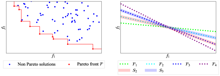
Figure 1: Conceptual visualizations of PF (Left) and EASs (Right). Both objectives $f_{1},f_{2}$ are better when they are lower. Left: an example of PF. The red dots in the objective space are the objective vectors that belong to PF $\mathcal{F}$ (the red solid line). The blue dots are dominated by the objective vectors in $\mathcal{F}$. In other words, the blue dots do not touch PF at all. Right: an example of EASs. Each dotted line represents four different PFs obtained by four independent runs. Weak-color bands show EASs of $L=2$ (red) and $L=3$ (blue). As can be seen, the red surface is attained by PFs from two independent runs, and the blue surface is attained by PFs from three independent runs.

2.3  Empirical Attainment Surface (EAS)

Suppose we obtained a set of PFs $\{\mathcal{F}_{s}\}_{s=1}^{S}$ from $S$ independent runs with a different random seed. EAS is defined by the following empirical attainment function:

$$\alpha(\bm{y})\coloneqq\alpha(\bm{y}\mid\mathcal{F}_{1},\dots,\mathcal{F}_{S})=\frac{1}{S}\sum_{s=1}^{S}\mathbb{I}[\mathcal{F}_{s}\preceq\bm{y}].$$ (2)

Intuitively speaking, if the empirical attainment function takes a certain integer $k(\leq S)$, $\bm{y}$ is dominated by $k$ different runs. Then $p\%$-EAS is defined as $\mathcal{S}\coloneqq\{\bm{y}\in\mathcal{Y}\mid\alpha(\bm{y})\geq p/100\}$. Since the percentages could take either of $\{100\times s/S\}_{s=0}^{S}$, EAS in the form of $\mathcal{S}_{L}\coloneqq\{\bm{y}\in\mathcal{Y}\mid\alpha(\bm{y})\geq L/S$ is used in practice. For example, $\mathcal{S}_{\lceil S/2\rceil}$ is PF achieved by half of the independent runs and $\mathcal{S}_{\lceil S/4\rceil}$ is PF achieved by a quarter of the independent runs. Using two different EASs, we can visualize the uncertainty of PF caused by random seeds. See Figure 1 for the intuition. If we have only a single objective, $\mathcal{S}_{\lceil S/2\rceil}$ has a unique value and this value is the median of the performance over $S$ independent runs.

3  Tool Usage

Our package is available at https://github.com/nabenabe0928/empirical-attainment-func and the package can be simply installed by pip install empirical-attainment-func. Throughout this section, we describe the usage of our package and use the following common code block:

⬇

rng = np.random.RandomState(0)

n_runs, n_samples, dim = 50, 20, 3

X = rng.random((n_runs, n_samples, dim)) * 10 - 5

# costs.shape = (n_runs, n_samples, 2)

# See Listing 4 in Appendix B for the definition

costs = func(X)

Note that n_runs, n_samples, and dim correspond to $S$, $N$, and $D$, respectively and we assume that each code block already imports numpy as np and matplotlib.pyplot as plt, and executes ax.legend() and plt.show() at the end for plotting.

3.1  Points on Empirical Attainment Surface

get_empirical_attainment_surface function computes EASs of the specified levels $L_{1},L_{2},\dots,L_{K}\in[1,S]$. This function takes the following arguments:

• costs (np.ndarray): an array of objective vectors in independent runs $\{\{\bm{f}(\bm{x}_{s,n})\}_{n=1}^{N}\}_{s=1}^{S}$ where $\bm{x}_{s,n}$ is the $n$-th HP in the $s$-th run,

• levels (List[int]): a list of levels $[L_{1},L_{2},\dots,L_{K}]$. If we use $[\lceil S/4\rceil,\lceil S/2\rceil,\lceil 3S/4\rceil]$, we get $[\mathcal{S}_{\lceil S/4\rceil},\mathcal{S}_{\lceil S/2\rceil},\mathcal{S}_{\lceil 3S/4\rceil}]$,

• larger_is_better_objectives (Optional[List[int]]): a list of integers to specify the objectives to be maximized (The default setting for each objective is minimization). For example, if we pass a list [1], the second objective is recognized as an objective to be maximized, and

• log_scale (Optional[List[int]]): a list of integers to specify the objectives to be handled in the log scale. For example, if we pass a list [1], the second objective is handled in the log scale.

An example usage is as follows:

Listing 1: An example of get_empirical_attainment_surface.

⬇

from eaf import get_empirical_attainment_surface

levels = [n_runs // 4, n_runs // 2, 3 * n_runs // 4]

# The arguments and output are explained in text

surfs = get_empirical_attainment_surface(costs, levels)

The output is, in principle, $[\mathcal{S}_{L_{1}},\mathcal{S}_{L_{2}},\dots,\mathcal{S}_{L_{K}}]$, but it is slightly different to handle the visualization easier. We first internally compute the union of PF solutions $P\coloneqq\cup_{s=1}^{S}\mathcal{P}_{s}$ for each independent run and yield all unique values in the first objective $F_{1}=\{f_{1}(\bm{x})\mid\bm{x}\in P\}\cup\{\infty,-\infty\}$. Each $\mathcal{S}_{L_{k}}$ for $k\in[K]$ has the shape of $(K,|F_{1}|,2)$ and the first element $y_{1}$ in $[y_{1},y_{2}]\coloneqq\bm{y}\in\mathcal{S}_{L_{k}}$ always takes a value in $F_{1}$. As the shapes of each $\mathcal{S}_{L_{k}}$ do not match each other without modifications, we pad the same value at the head of each $\mathcal{S}_{L_{k}}$ with an edge point of $\mathcal{S}_{L_{k}}$ so that $\mathcal{S}_{L_{k}}$ only includes the observations at EAS. By connecting nodes in $\mathcal{S}_{L_{k}}$, we can visualize EAS with the level of $L_{k}$. Note that $\mathcal{S}_{L_{k}}$ is sorted by $y_{1}$ in $[y_{1},y_{2}]\coloneqq\bm{y}\in\mathcal{S}_{L_{k}}$ by default.

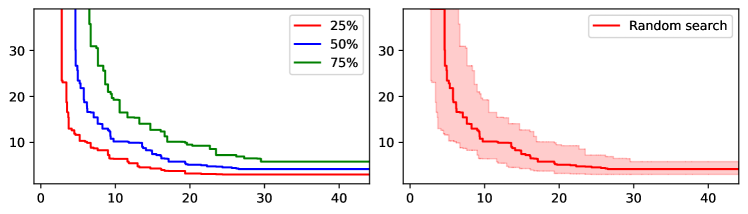
Figure 2: The visualizations obtained by Listing 2 (Left) and Listing 3 (Right). The horizontal axis shows $f_{1}$ and the vertical axis shows $f_{2}$. Left: an example of plots of EASs. By repeating the same process for different MOO methods, we can easily compare with various methods. Right: an example of a plot of EAS with the uncertainty band. The weak-color band shows the variability of PF caused by random seeds.

3.2  Plot of Empirical Attainment Surfaces

For plots, we use EmpiricalAttainmentFuncPlot and it receives the following arguments for internal processing:

• larger_is_better_objectives (Optional[List[int]]): Same as in Section 3.1,

• log_scale (Optional[List[int]]): Same as in Section 3.1,

• true_pareto_sols (Optional[np.ndarray]): an array of the true PF if available. It is required if we plot normalized HV,

• x_min,x_max,y_min,y_max (float): the lower/upper bounds of the first/second objective if available. These values could be used to fix the value ranges of each objective, and

• ref_point (np.ndarray): the reference point of the problem of interest if available. It is required if we plot HV (see Appendix B).

Although all of them are optional, additional information could enable extra plots such as HV and the surface of PF. Assuming that we already computed surfs ($[\mathcal{S}_{\lceil S/4\rceil},\mathcal{S}_{\lceil S/2\rceil},\mathcal{S}_{\lceil 3S/4\rceil}]$) from the previous section, then we can connect the nodes in $\mathcal{S}_{L_{k}}$ simply by the following:

Listing 2: An example of plot_multiple_surface.

⬇

from eaf import EmpiricalAttainmentFuncPlot

_, ax = plt.subplots()

eaf_plot = EmpiricalAttainmentFuncPlot()

colors = ["red", "blue", "green"]

labels = ["25%", "50%", "75%"]

eaf_plot.plot_multiple_surface(

ax, colors=colors, labels=labels, surfs=surfs

)

The figure generated by this code is available in Figure 2 (Left). We need to pass ax and surfs for plot. On top of them, this function requires colors and labels, and we can optionally pass linestyles, markers, and kwargs for ax.plot. Each argument is a list of arguments used in ax.plot. If we need to plot only a single EAS, eaf_plot.plot_surface could be used instead. When we would like to visualize the uncertainty band of PF, plot_surface_with_band or plot_multiple_surface_with_band could be used:

Listing 3: An example of plot_surface_with_band.

⬇

eaf_plot.plot_surface_with_band(

ax, color="red", label="Random search", surfs=surfs

)

Note that surfs for plot_surface_with_band and each element in surfs_list for plot_multiple_surface_with_band must be an array with the shape of $(K,|F_{1}|,2)$ where $K=3$ and $\mathcal{S}_{L_{1}},\mathcal{S}_{L_{2}},\mathcal{S}_{L_{3}}$ will determine the lower/upper bound of the band and the center line. Figure 2 (Right) visualizes the result obtained by this code. In Figure 2 (Left), the red line corresponds to $\mathcal{S}_{L_{1}}$, the blue line corresponds to $\mathcal{S}_{L_{2}}$, and the green line corresponds to $\mathcal{S}_{L_{3}}$. We can easily plot EASs of various MOO methods using plot_multiple_surface_with_band as well.

4  Conclusions

In this paper, we introduced a Python package to visualize uncertainty bands for MOO. As described, our package is very easy to use and users can easily get the observations on EAS and EAS itself. Although recent research papers often focus on the visualization of HV over time or PF from a single run, this easy-to-use package allows researchers to qualitatively evaluate the uncertainty in their MOO methods and potential readers would not be left behind due to the lack of interpretability caused by the information loss either from HV or choosing a single random seed.

Appendix A Hypervolume (HV)

HV is a widely used metric to compare the performance of various MOO methods. To compute HV of a set of observations $\mathcal{D}$, we first define a reference point $\bm{r}\in\mathbb{R}^{M}$ so that the reference point is dominated by all the observations in $\mathcal{D}$. More formally, the reference point is chosen from a set $\bm{r}\in\{\bm{y}\in\mathbb{R}^{M}\mid f(\bm{x}_{n})\prec\bm{y}\}$. In practice, if users already know the possible worst (in our case maximum) value for each objective, these values will be used. Then HV is defined as follows:

Definition 4 (Hypervolume (HV))

Suppose $\mu$ is the Lebesgue measure defined on $\mathbb{R}^{M}$ and $\mathcal{F}$ is PF in the objective space $\mathcal{Y}$, then HV is computed as:

$$V(\mathcal{F}|\bm{r})\coloneqq\mu(\{\bm{y}\in\mathbb{R}^{M}\mid\mathcal{F}\prec\bm{y}\prec\bm{r}\}).$$ (3)

Roughly speaking, the Lebesgue measure quantifies the volume of an input. Note that HV is invariant to the normalization, i.e. to transform each objective’s range into $[0,1]$, and thus normalized HV is used in practice.

Although HV is a convenient metric for comparison, high HV does not guarantee that MOO methods yielded a diverse set of solutions. For example, let the reference point $\bm{r}=[1.1,1.1]$ and $f_{1},f_{2}$ be mappings $\mathcal{X}\rightarrow[0,1]\times[0,1]$. If $f_{1}$ is uniformly distributed in $0\leq f_{1}\leq 10^{-5}$ while $f_{2}$ is uniformly distributed in $[0,1]$ in the objective space, although $f_{1}\leq 10^{-7}$ is the top-$1\%$ solution, HV variates with the scale of $(1.1-10^{-7})/(1.1-10^{-5})\simeq 1$ in comparison to a set of trivial solutions. On the other hand, when we yield the top-$1\%$ solution in $f_{2}$, which is $0.01$, HV variates with the scale of $(1,1-0.01)/(1.1-1)=10.9$. In other words, we could focus on the optimization of $f_{2}$ if we would like to hack the visualization with HV. From this example, we can easily recognize the potential problems that HV might cause due to its heavy dependency on the choice of the reference point $\bm{r}$ and the distribution of the objective vector $p(\bm{y})$. This example also implies that the reference point must be as small as possible and the standard error taken over multiple independent runs could be extremely small depending on the distribution $p(\bm{y})$.

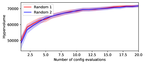
Figure 3: The visualizations obtained by Listing 4. This example is a plot of HV over time with the uncertainty band of the standard error.

Appendix B Hypervolume Plot over Time

Figure 3 Our package also supports the plot of HV for $M=2$ over time.

Listing 4: An example of plot_multiple_hypervolume2d_with_band.

⬇

X2 = rng.random((n_runs, n_samples, dim)) * 10 - 5

costs2 = func(X2)

stacked_costs = np.stack([costs, costs2])

ref_point = np.array([75, 1029]) # problem specific

eaf_plot = EmpiricalAttainmentFuncPlot(

ref_point=ref_point

)

colors = ["red", "blue"]

labels = ["Random 1", "Random 2"]

eaf_plot.plot_multiple_hypervolume2d_with_band(

ax,

costs_array=stacked_costs,

colors=colors,

labels=labels,

normalize=False,

)

We can use the normalize option only if we have the true set of PF.

References

- Awad et al., (2023) Awad, N., Sharma, A., and Hutter, F. (2023). MO-DEHB: Evolutionary-based Hyperband for multi-objective optimization. arXiv:2305.04502.
- Chen et al., (2018) Chen, Y., Huang, A., Wang, Z., Antonoglou, I., Schrittwieser, J., Silver, D., and de Freitas, N. (2018). Bayesian optimization in AlphaGo. arXiv:1812.06855.
- Deb et al., (2002) Deb, K., Pratap, A., Agarwal, S., and Meyarivan, T. (2002). A fast and elitist multiobjective genetic algorithm: NSGA-II. Evolutionary Computation, 6.
- Fonseca et al., (2011) Fonseca, C., Guerreiro, A., López-Ibánez, M., and Paquete, L. (2011). On the computation of the empirical attainment function. In International Conference on Evolutionary Multi-Criterion Optimization.
- Henderson et al., (2018) Henderson, P., Islam, R., Bachman, P., Pineau, J., Precup, D., and Meger, D. (2018). Deep reinforcement learning that matters. In AAAI Conference on Artificial Intelligence.
- Knowles, (2005) Knowles, J. (2005). A summary-attainment-surface plotting method for visualizing the performance of stochastic multiobjective optimizers. In International Conference on Intelligent Systems Design and Applications.
- Kruskal and Wish, (1978) Kruskal, J. and Wish, M. (1978). Multidimensional scaling, volume 11.
- Kung et al., (1975) Kung, H., Luccio, F., and Preparata, F. (1975). On finding the maxima of a set of vectors. Journal of the ACM, 22.
- Mead, (1992) Mead, A. (1992). Review of the development of multidimensional scaling methods. Journal of the Royal Statistical Society: Series D (The Statistician), 41.
- Ozaki et al., (2022) Ozaki, Y., Tanigaki, Y., Watanabe, S., Nomura, M., and Onishi, M. (2022). Multiobjective tree-structured Parzen estimator. Journal of Artificial Intelligence Research, 73.
- Ozaki et al., (2020) Ozaki, Y., Tanigaki, Y., Watanabe, S., and Onishi, M. (2020). Multiobjective tree-structured Parzen estimator for computationally expensive optimization problems. In Genetic and Evolutionary Computation Conference.
- Tušar and Filipič, (2013) Tušar, T. and Filipič, B. (2013). An approach to visualizing the 3D empirical attainment function. In Genetic and Evolutionary Computation Conference.
- Watanabe et al., (2022) Watanabe, S., Awad, N., Onishi, M., and Hutter, F. (2022). Multi-objective tree-structured Parzen estimator meets meta-learning. arXiv:2212.06751.
- Watanabe et al., (2023) Watanabe, S., Awad, N., Onishi, M., and Hutter, F. (2023). Speeding up multi-objective hyperparameter optimization by task similarity-based meta-learning for the tree-structured Parzen estimator. arXiv:2212.06751.